Cosmological constraints on dark matter annihilation and decay: Cross-correlation analysis of the extragalactic -ray background and cosmic shear
Abstract
We derive constraints on dark matter (DM) annihilation cross section and decay lifetime from cross-correlation analyses of the data from Fermi-LAT and weak lensing surveys that cover a wide area of squared degrees in total. We improve upon our previous analyses by using an updated extragalactic -ray background data reprocessed with the Fermi Pass 8 pipeline, and by using well-calibrated shape measurements of about twelve million galaxies in the Canada-France-Hawaii Lensing Survey (CFHTLenS) and Red-Cluster-Sequence Lensing Survey (RCSLenS). We generate a large set of full-sky mock catalogs from cosmological -body simulations and use them to estimate statistical errors accurately. The measured cross correlation is consistent with null detection, which is then used to place strong cosmological constraints on annihilating and decaying DM. For leptophilic DM, the constraints are improved by a factor of in the mass range of TeV when including contributions from secondary rays due to the inverse-Compton upscattering of background photons. Annihilation cross-sections of are excluded for TeV-scale DM depending on channel. Lifetimes of sec are also excluded for the decaying TeV-scale DM. Finally, we apply this analysis to wino DM and exclude the wino mass around 200 GeV. These constraints will be further tightened, and all the interesting wino DM parameter region can be tested, by using data from future wide-field cosmology surveys.
I INTRODUCTION
An array of astronomical observations over a wide range of redshifts and length scales consistently support the existence of cosmic dark matter (DM). Recent observations include the statistical analysis of the cosmic microwave background (CMB) anisotropies (e.g., Refs. Hinshaw et al. (2013); Ade et al. (2014)), spatial clustering of galaxies (e.g., Ref. Eisenstein et al. (2005)), galaxy rotation curves (e.g., Ref. Persic et al. (1996)), and direct mapping of matter distribution through gravitational lensing (e.g., Ref. Clowe et al. (2006)).
Gravitational lensing is a direct and most promising probe of the matter density distribution in the Universe. A foreground gravitational field causes small distortions of the images of distant background galaxies. The small distortions contain, collectively, rich information on the foreground matter distribution and its growth over cosmic time. In the past decades, the coherent lensing effect between galaxy pairs with angular separation of degree has been successfully detected in wide-area surveys (e.g., Refs Bacon et al. (2000); Kilbinger et al. (2013); Becker et al. (2015)). Most importantly, the large angular scale signals, called cosmic shear, probe the matter distribution in an unbiased manner. However, cosmic shear alone does not provide, by definition, any information on possible electromagnetic signatures from DM, and thus it cannot be used to probe the particle properties of DM such as annihilation cross section and decay lifetime.
The extragalactic -ray background is thought to be a potential probe of DM, if DM annihilates or decays to produce high-energy photons. Weakly interacting massive particles (WIMPs) are promising DM candidates that can naturally explain the observed abundance of cosmic DM if the WIMP mass ranges from 10 GeV to 10 TeV and the self-annihilation occurs around the weak-interaction scale Jungman et al. (1996). Dark matter decay lifetime remains largely unknown, and, in fact, there are not strong cosmological and astrophysical evidences for stable DM; the possibility of very long-lived particles with a lifetime longer than the age of the Universe of 13.8 Gyr remains viable. DM annihilation or decay produces a variety of cascade products and thus leaves characteristic imprints in, for example, the cosmic -ray background. The isotropic -ray background (IGRB) is a promising target to search for DM annihilation or decay Funk (2015). Although the mean IGRB intensity can be explained by (extrapolating) unresolved astrophysical sources (e.g., Ajello et al. (2015)), there remains substantial uncertainties and thus there is room for contribution from other unknown sources. The anisotropies in the diffuse -ray background should in principle contain rich information about DM contributions at small and large length scales (e.g., see Ref. Fornasa and Sánchez-Conde (2015) for review).
It has been proposed that the cross-correlation of the IGRB with large-scale structure provides a novel probe of the microscopic properties of DM Camera et al. (2013); Fornengo and Regis (2014); Ando et al. (2014); Ando (2014); Camera et al. (2015). Positive correlations with actual galaxy survey data Xia et al. (2015) have been reported, and implications for the nature of DM have been discussed Regis et al. (2015); Cuoco et al. (2015).
In this paper, we search indirect DM signals through cross-correlation of the IGRB and cosmic shear. We improve the cross-correlation measurement over our previous analysis Shirasaki et al. (2014) by using the latest -ray data taken from the Fermi-LAT and two publicly available galaxy catalogs, the Canada-France-Hawaii Lensing Survey (CFHTLenS) and the Red-Cluster-Sequence Lensing Survey (RCSLenS), that provide with precise galaxy shape measurement. We apply a set of Galactic -ray emission models to characterize the foreground emission from our own Galaxy, and also utilize full-sky simulations of cosmic shear to construct realistic mock galaxy catalogues specifically for CFHTLenS and RCSLenS. In order to make the best use of the cross-correlation signals over a wide range of angular separations, we calculate the statistical uncertainties associated with the intrinsic galaxy shapes, the Poisson photon noise, and the sample variance of cosmic shear. To this end, we make use of our large mock catalogues in a manner closely following the actual observations. The methodology presented in this paper is readily applicable to cross-correlation analyses of the IGRB and cosmic shear with ongoing and future surveys, such as the Hyper-Suprime Cam, the Dark Energy Survey, the Large Synoptic Survey Telescope, and the Cherenkov Telescope Array.
The rest of the paper is organized as follows. In Section II, we summarize the basics of the two observables of interest: IGRB and cosmic shear. We also present a theoretical model of the cross-correlation of the IGRB and cosmic shear in annihilating or decaying DM scenarios. In Section III, we describe the -ray data and the galaxy imaging survey for shape measurement. The details of the cross-correlation analysis are provided in Section IV. In Section V, we show the result of our cross-correlation analysis, and derive constraints on particle DM. Concluding remarks and discussions are given in Section VI. Throughout the paper, we adopt the standard CDM model with the following parameters; matter density , dark energy density , the density fluctuation amplitude , the parameter of the equation of state of dark energy , Hubble parameter and the scalar spectral index . These parameters are consistent with the WMAP nine-year results (Hinshaw et al., 2013).
II A MODEL OF DARK MATTER
II.1 Extragalactic probe
We consider two observables to probe dark matter properties: the IGRB and cosmic shear. The former may contain rays from DM annihilation/decay located outside of our galaxy, while the latter provides unbiased information of the DM mass distribution in the Universe.
Isotropic -ray background
The IGRB intensity is defined by the number of photons per unit energy, area, time, and solid angle,
| (1) |
where is the observed -ray energy, is the energy of the ray at redshift , is the Hubble parameter in a flat Universe, and the exponential factor in the integral takes into account the effect of -ray attenuation during propagation owing to pair creation on diffuse extragalactic photons. For the -ray optical depth , we adopt the model in Ref. (Gilmore et al., 2012). In Eq. (1), represents the volume emissivity (i.e., the photon energy emitted per unit volume, time, and energy range), which is given by
| (2) |
where is a -ray source function and represents the relevant density field of -ray sources.
Here we consider two particle properties of DM, annihilation and decay. For annihilating DM, the two functions and are given by
| (3) | |||||
| (4) |
where is the -ray spectrum per annihilation, describes the -ray energy distribution through the inverse-Compton (IC) scattering between produced by annihilation and background photons, is the annihilation cross section times the relative velocity averaged with the velocity distribution function, and is the DM particle mass. For decaying dark matter,
| (5) | |||||
| (6) |
where is the -ray spectrum per decay, is the contribution from the inverse-Compton scattering of decay products , and is the decay rate. Note that we assume the same source distributions of the primary and secondary photons in this paper. The source distribution of secondary photons can differ from that of primary photons, because the annihilation/decay products can propagate or diffuse while they produce secondary photons. The diffusion time scale of electrons with 100 GeV is much longer than the cooling time scale due to inverse-Compton energy losses in both galaxy-sized and cluster-sized haloes Ishiwata et al. (2009); Brunetti and Jones (2014). We can safely ignore the propagation effect of sources of secondary photons in our halo model approach.
We assume that the IGRB intensity is measured in the energy range to along a given angular direction . The DM contribution in Eq. (1) is given by
| (7) | |||||
| (8) |
where is the comoving distance. Throughout this paper, we set and , respectively.
Cosmic shear
Images of distant galaxies are distorted by the weak lensing effect due to foreground matter distributions. The weak lensing effect is commonly characterized by the following two-dimensional matrix;
| (11) |
where is the convergence, is shear, and and represent the observed position and the true position of a source object, respectively.
When considering the metric perturbation in the Newtonian gauge, one finds that each component of can be related to the second derivative of the gravitational potential Bartelmann and Schneider (2001). Since the gravitational potential can be related to the matter density through the Poisson equation, the convergence field is expressed as
| (12) |
where is the matter overdensity field. The weight in Eq. (12) is given by
| (13) | |||||
where is the comoving distance to the horizon, is the comoving angular diameter distance, and represents the source distribution normalized to .
II.2 Microscopic processes
DM annihilation or decay generally yields a mixture of various final states depending upon the particle interaction model. We consider three benchmark models with % branching ratios to , , and final states; in Section V.2 we also explore a specific model of wino DM. We use the PPPC4DMID package (Cirelli et al., 2011) to estimate the primary -ray energy spectrum. For and final states, hadronic production of neutral pions are kinematically allowed and the -ray spectra are dominated by the decay of neutral pions. For decaying DM with particle mass of , we model the -ray spectrum per decay () using the -ray spectrum from annihilation () except with a particle mass of . These are primary -ray emissions, to be distinguished from secondary emission that results from interactions of the annihilation products with the environment.
An example of a relevant secondary emission is the inverse-Compton -rays that are up-scattered background photons off of the high energy produced through annihilation or decay or subsequent interactions. We follow Refs. Ando and Ishiwata (2015, 2016) to calculate the inverse-Compton contributions from up-scattered photons, i.e., in Eq. (3) and in Eq. (5). The energy spectrum of the inverse-Compton -rays can be expressed as Ishiwata et al. (2009); Ando and Ishiwata (2015, 2016)
| (14) | |||||
with for annihilation and decay, respectively. Here, and represent the energy of and the background photons, is the energy spectrum of the background photon field, is the differential cross section of the inverse-Compton scattering, and is the energy loss rate of . In Eq. (14), is defined by
| (15) |
where is the energy distribution of produced by DM annihilation or decay . We consider the CMB as the background photons and ignore the extragalactic background light (EBL) with other wavelengths. Ref. Ando and Ishiwata (2016) has shown that the EBL would only have a contribution to the energy loss rate of at , and even less at higher . In order to calculate the energy spectrum of inverse-Compton -rays, we need the energy distribution of in annihilation/decays, which we calculate using PPPC4DMID (Cirelli et al., 2011) for each of our adopted final states.
For CMB, the integrand of Eq. (14) has a maximum at eV and for GeV. Hence heavy DM with mass GeV would be needed for prominent secondary -ray emissions, because the integrand is proportional to the cumulative number of given by Eq. (15). For GeV, we find the maximum in the integrand of Eq. (14) to be at eV, and thus , suggesting that DM with mass of GeV yields a larger secondary contribution than the primary one at GeV. Therefore, setting a low energy cut in -ray analysis would be important to efficiently search for cross-correlation signals from DM annihilation or decay with GeV. In practice, we use the rays with GeV in our analyses, because the smearing effect of Fermi’s point spread function (PSF) on cross-correlation analysis is significant in the range of GeV at present.
II.3 Cross-correlation statistics
Using Eqs. (7) and (12), with the Limber approximation Limber (1954), we can calculate the angular cross-power spectrum of the convergence field and extragalactic rays emitted through DM annihilation/decay as,
| (16) | |||||
where represents the three-dimensional power spectrum between two fields of and as a function of wave number and redshift .
In practice, a more direct observable is the two-point cross-correlation function of the tangential shear and -ray intensity Shirasaki et al. (2014). The two-point cross-correlation function can be calculated from the angular power spectrum by the following equation:
| (17) |
where represents the second-order Bessel function (de Putter and Takada, 2010; Oguri and Takada, 2011). Furthermore, the smearing effect of Fermi’s PSF on would be relevant to the -ray statistics on small angular scales. Thus, we apply the same framework to take into account the PSF effect, as in Ref. Shirasaki et al. (2014).
For annihilation, in Eq. (16) is equivalent to where is the mean DM density at redshift and represents the cross power spectrum of matter overdensity and its squared. We adopt the halo model approach to predict as in Ref. Shirasaki et al. (2014). In the framework of the halo model Cooray and Sheth (2002), can be expressed as a sum of two terms, called the one-halo and two-halo term, respectively. The former represents the two-point correlation within a given DM halo, and the latter corresponds to the clustering of DM halos. In the halo-model calculation, we adopt the model of halo mass function and linear halo bias as in Refs. Tinker et al. (2008, 2010), and assume the NFW density profile Navarro et al. (1997) with concentrations as given in Ref. Prada et al. (2012). For the boost factor that describes the effective increase of the amplitude of the DM density clumping, we consider two phenomenological models by Refs. Gao et al. (2012); Sánchez-Conde and Prada (2014). In one model, subhalo properties are scaled as power laws and extrapolated many orders of magnitudes to the smallest subhalos () Gao et al. (2012). This procedure yields a large boost factor, but it is rather uncertain whether the extrapolation remains valid to such small halos. We thus test another model as an optimistic scenario, where the halo concentration is given by a relation that flattens at small halo masses, yielding a smaller boost factor Sánchez-Conde and Prada (2014). We regard the latter model as a conservative case, because the concentration-mass relation is derived from field halos rather than subhalos. For a given mass, a subhalo is expected to be more concentrated than a field halo, and hence the boost factor in the latter model remains modest. Ref. Bartels and Ando (2015) estimates that the net effect is a factor of 2–5 increase in of Ref. Sánchez-Conde and Prada (2014).
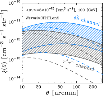
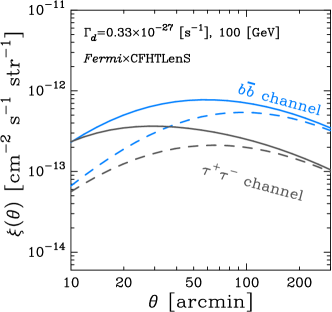
Fig. 1 shows our benchmark model of . Here, we consider two representative channels ( and ) for a 100 GeV DM, and only show the primary -ray contribution. The top panel shows the case of annihilating DM with a thermal cross section . We also show the model uncertainty originating from the choice of the boost factor. The expected correlation for each channel lies in the shaded region in the top panel. The uncertainty of the boost factor causes an uncertainty in of a factor of for annihilating DM. Our model predicts that the contribution from inside a single DM halo (i.e., arising from subhalos) dominate on scale of arcmin, while the clustering of DM halos induce significant correlations at deg.
For decaying DM, in Eq. (16) is given by , where is the three-dimensional power spectrum of the matter overdensity. The power spectrum has been calibrated with a set of N-body simulations over a wide range of and for cosmological analyses. We adopt a fitting formula of that reproduces the nonlinear effects on two-point statistics at scales, consistently with the result of cosmological N-body simulations Takahashi et al. (2012). For comparison, we also calculate the cross-correlation adopting linear matter power spectrum.
The bottom panel of Fig. 1 shows the case of decaying DM with decay rate of . There, the solid lines represent the model with nonlinear power spectrum , while the dashed lines are with linear . We find that the nonlinear gravitational growth enhances the signal at arcmin scales by a factor of a few. The linear approximation is valid only at scales larger than a few degrees.
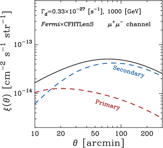
We next consider the effect of secondary rays on our cross-correlation statistics . Fig. 2 summarizes the contributions for a 1 TeV dark matter decaying into final states. The red line shows the correlation signals originating from primary rays, while the blue line is for the secondary contribution produced by the inverse-Compton scattering of CMB photons by the decay products . As shown in Fig. 2, the secondary rays dominate the cross-correlation statistics when large amounts of energetic leptons are generated, as in the case of heavy DM particles with 1-10 TeV masses annihilating/decaying in leptonic channels. The different angular dependence between the red and blue lines originates from the energy dependence of the -ray PSF. The primary rays have a dominant contribution to the IGRB intensity for GeV, while the secondary mainly contributes to observed photon counts with lower energies of GeV Ando and Ishiwata (2016). Since the size of the -ray PSF is smaller for higher energy photons, the secondary contribution tends to be affected more by the PSF smoothing than the primary contribution.
III DATA
III.1 Fermi-LAT data selection and methodology
The Fermi-LAT detects -ray photons in the energy range 20 MeV to over 300 GeV (Atwood et al., 2009). In operation since August 2008, this telescope makes all sky observations every hours, making it an excellent tool to investigate diffuse -ray background photons. The LAT instrument is described in detail in Ref. (Atwood et al., 2009).
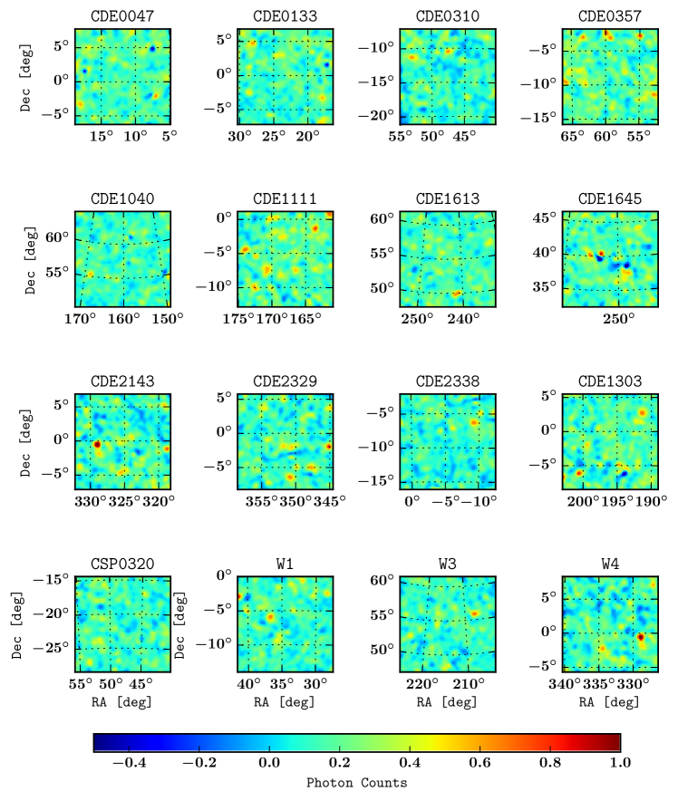
The analysis presented here was carried out with years of observations from August 4, 2008September 4, 2015 of the recently released Pass 8 data. For each CFHTLens and RCSLens patch, we selected events within a squared region of (around their respective centroids) with energies greater than 1 GeV, and using combined Front and Back events. At low energies the angular resolution of the LAT is poor and source confusion could introduce a bias in the analysis, the chosen low energy limit is a compromise between sensitivity and statistics.
Events and instrument response functions (IRFs) for the lowest-residual cosmic ray (CR) background “ULTRACLEANVETO” 111ULTRACLEANVETO events are the recommended class of photons for investigation of the IGRB at intermediate to high latitudes. The reader is referred to the Cicerone (http://fermi.gsfc.nasa.gov/ssc/data/analysis/documentation/Pass8_usage.html) for further details from the Pass 8 were used. The zenith angles were chosen to be smaller than 100∘ to reduce contamination from the Earth limb. Time intervals when the rocking angle was more than 52∘ and when the Fermi satellite was within the South Atlantic Anomaly were also excluded.
In order to determine the IGRB photons in all of the CFHTLens and RCSLens region of interest (ROI) we performed a maximum-likelihood fit (Acero et al., 2015) with the pyLikelihood analysis tool 222 http://fermi.gsfc.nasa.gov/ssc/data/analysis/documentation/. The energy binning was set to 24 logarithmic evenly spaced bins and the Fermi Science Tools 333http://fermi.gsfc.nasa.gov/ssc/data/analysis/ v10r0p5 was used.
In the fit we employed all 3FGL (Acero et al., 2015) -ray point-sources present in each ROI plus the standard diffuse Galactic background (DGB) gll-iem-v06.fits and the isotropic extra-galactic background model iso-P8R2-ULTRACLEANVETO-V6-v06.txt. In addition, we included specialized templates for the Sun and Moon in our fits. These account for diffuse -ray photons resulting from CR interactions with the solar radiation field, solar atmosphere, and the lunar lithosphere. The Sun and Moon templates were constructed by making use of the tool gtsuntemp as explained in the Cicerone 444 http://fermi.gsfc.nasa.gov/ssc/data/analysis/scitools/solar_template.html.
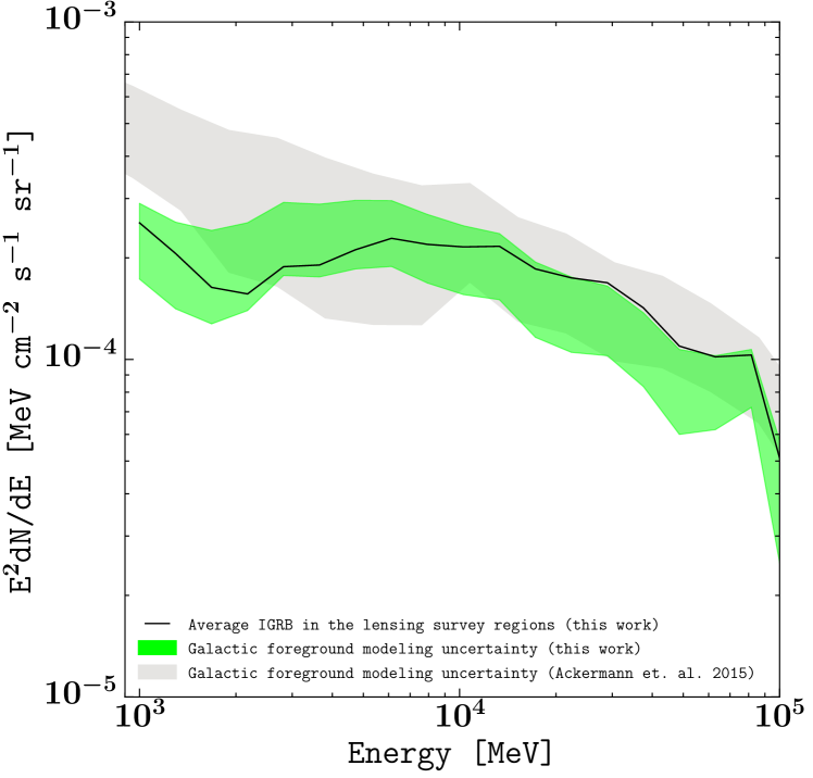
The normalization and spectral index of all the -ray point sources that fell within of the center of each patch were left free in the fit while all the spectral parameters of sources which were within of the ROI perimeter were fixed to their catalog values (Acero et al., 2015). We also varied the normalizations corresponding to the isotropic and DGB components but kept the Sun and Moon fluxes fixed to their nominal values. Convergence was reached iteratively by following a relaxation method that has proven to be successful in a region with a high density of -ray point sources and large parameter degeneracies (Macias and Gordon, 2014; Abazajian et al., 2014). Lastly, the extragalactic diffuse photons were obtained by subtracting the best-fit DGB and point sources from the raw counts maps. A mosaic with the resulting IGRB residual images is shown in Fig. 3. Note that the residual obtained in this way in principle contains also isotropic detector backgrounds. The normalization of the isotropic extragalactic background template is typically about 0.6–0.7. However, we are able to reproduce well the IGRB derived by the Fermi collaboration Ackermann et al. (2015) as shown in Figure 5. From this we conclude that detector backgrounds are safely removed by our conservative photon selection and zenith angle cuts. As described in Section IV.3, we examine multiple templates for the Galactic diffuse emission model, whose uncertainties can dominate analyses of residuals. Nevertheless, we find that the statistical uncertainty would dominate the systematic uncertainties in the diffuse modeling in the current survey. The details are found in Section IV.3.
III.2 CFHTLenS and RCSLenS
We use the cosmic shear data from the Canada-France-Hawaii Telescope Lensing Survey (CFHTLenS) Heymans et al. (2012) and the Red Cluster Sequence Lensing Survey (RCSLenS) Hildebrandt et al. (2016). Table 1 summarizes the number of source galaxies and the effective survey area for each subregion used in the present paper.
| Survey | Name of patch | Effective area () | |
|---|---|---|---|
| W1 | 2,570,270 | 63.6 | |
| W3 | 1,649,718 | 41.5 | |
| W4 | 770,356 | 21.2 | |
| CFHTLenS | 4,990,344 | 126.3 | |
| CDE0047 | 954,554 | 55.2 | |
| CDE0133 | 430,775 | 27.8 | |
| CDE0310 | 101,851 | 68.7 | |
| CDE0357 | 455,616 | 27.7 | |
| CDE1040 | 429,987 | 27.6 | |
| CDE1111 | 1,075,176 | 67.7 | |
| CDE1303 | 229,533 | 13.4 | |
| CDE1613 | 381,365 | 24.9 | |
| CDE1645 | 404,837 | 24.0 | |
| CDE2143 | 1,178,282 | 71.1 | |
| CDE2329 | 691,348 | 38.9 | |
| CDE2338 | 1,070,288 | 64.9 | |
| CSP0320 | 436,054 | 22.8 | |
| RCSLenS | 7,839,666 | 534.7 | |
| TOTAL | 12,830,010 | 661.0 |
CFHTLenS
CFHTLenS is a 154 square degree multi-color optical survey in five optical bands . CFHTLenS is optimized for weak lensing analysis with a full multi-color depth of with optimal sub-arcsec seeing conditions. The survey consists of four separated regions called W1, W2, W3, and W4, with an area of 72, 30, 50, and 25 square degrees, respectively.
In CFHTLenS, catalog construction mainly consists of the following three processes: photometric redshift measurement (Hildebrandt et al., 2012), weak lensing data processing with THELI (Erben et al., 2013), and shear measurement with fit (Miller et al., 2013). A detailed systematic error study of the shear measurements in combination with the photometric redshifts is presented in Ref. (Heymans et al., 2012) and additional error analyses of the photometric redshift measurements are presented in Ref. (Benjamin et al., 2013).
The ellipticities of the source galaxies in the data have been calculated using the fit algorithm. fit performs a Bayesian model fitting to the imaging data by varying a galaxy’s ellipticity and size, and by marginalizing over the centroid position. It adopts a forward convolution process that convolves the galaxy model with the PSF to estimate the posterior probability of the model given the data. For each galaxy, the ellipticity is estimated as the mean likelihood of the model posterior probability after marginalizing over galaxy size, centroid position, and bulge fraction. An inverse variance weight is given by the variance of the ellipticity likelihood surface and the variance of the ellipticity distribution of the galaxy population (see Ref. (Miller et al., 2013) for further details).
The photometric redshifts are estimated by the BPZ code Benitez (2000). The true redshift distribution of sources is well described by the sum of the probability distribution functions (PDFs) estimated from BPZ (Benjamin et al., 2013). The galaxy-galaxy-lensing redshift scaling analysis confirms that contamination is not significant for galaxies selected at (Heymans et al., 2012). In this redshift range, the weighted median redshift is and the effective weighted number density is 11 per square arcmins. We have used the source galaxies with to measure the cross-correlation of cosmic shear and IGRB.
To make a reliable lensing measurement, we use the following criteria of source galaxies in addition to the selection of redshift. First, we discard galaxies that have the flag , indicating masked objects. We use the galaxies that have ellipticity weight , and the ellipticity fitting flag , which indicates that the shape is reliably estimated.
RCSLenS
RCSLenS fully utilizes multiband imaging data taken by the Red-sequence Cluster Survey 2 (RCS2) Gilbank et al. (2011). RCS2 is a 785 square degree multi-color imaging survey with sub-arcsecond seeing in four bands to a depth of mag in the -band and originally designed to optically select a very large sample of galaxy clusters over a wide redshift range. RCSLenS reanalyzes the imaging data in RCS2 with a dedicated weak lensing pipeline examined in the CFHTLenS survey. RCSLenS consists of 14 separate regions with varying survey area between square degrees.
The lensing data in RCSLenS is obtained by reanalysis of RCS2 imaging data with THELI and fit, as in CFHTLenS. The effective source number density in RCSLenS is per square arcmins. The photometric redshift estimates by BPZ are only derived for pointings with four-color information, corresponding to about two-thirds of the survey area. Ref. Harnois-Déraps et al. (2016) has estimated the underlying source redshift distribution by using the CFHTLenS sample incorporated with near-IR and GALEX near-UV data. This new photometric sample, called CFHTLenS-VIPERS, is calibrated against 60,000 spectroscopic redshifts Coupon et al. (2015). The source redshift distribution in RCSLenS then has been constructed with stacking of the photometric redshift PDF over the CFHTLenS-VIPERS galaxies that pass the same RCSLenS selection criteria. The resulting redshift distribution can be fitted by the sum of exponential functions with nine free parameters and the median redshift is found to be . The detailed function form and best-fitted parameters are summarized in Ref. Harnois-Déraps et al. (2016).
For the RCSLenS, we perform the same selection of source galaxies as in the case of CFHTLenS; removal with and selection with and . In addition, we adopt the selection in -band magnitude of , as in Ref. Harnois-Déraps et al. (2016).
IV CROSS CORRELATION
IV.1 Measurement
In order to detect the cross-correlation signal of IGRB and cosmic shear, we introduce the following estimator Shirasaki et al. (2014),
| (18) |
where is the observed IGRB intensity in pixel of the -ray map, is the weight related to the shape measurement, and is the tangential component of the -th galaxy’s ellipticity, defined by
| (19) | |||||
where is defined as the angle measured from the right ascension direction to a line connecting the -th pixel and the -th galaxy. The overall factor in Eq. (18) is used to correct for the multiplicative shear bias in the shape measurement with fit (Miller et al., 2013). It is given by
| (20) |
For binning in angular separation , we employ a logarithmically equally spaced binning in the range of 10 – 300 arcmin. The number of bins is set to be 10.
In order to quantify the systematics in the shape measurement, we consider the cross-correlation using another component of weak lensing shear that is rotated from the tangential shear component. We denote this shear component . This is commonly used as an indicator of systematics in the shape measurement, since the correlation signal with should vanish statistically in the case of shape measurement and no intrinsic alignment. In addition, Eq. (18) should be dependent on the details of the subtraction of Galactic rays from the observed photon count maps. We take into account this systematic uncertainty by using different models of the Galactic -ray foreground emission. The details of the analyses are summarized in Section IV.3.
IV.2 Statistical uncertainties
To discuss the statistical significance of the measured estimator from real data, we need to estimate the covariance of Eq. (18). According to Ref. Shirasaki et al. (2014), the covariance in the case of can be expressed as
| (21) |
where represents the covariance associated with the intrinsic shape of source galaxies and the Poisson noise of photon counts, is the contribution of the sample variance of cosmic shear and photon noise, stands for the covariance originated from the intrinsic shape and the angular correlation of observed photon counts, and is the covariance caused by the sample variance of cosmic shear and the angular correlation of observed photon counts.
Since the cosmic shear is time smaller than the intrinsic shape of sources (called shape noise) in the current ground-based galaxy imaging survey, the two terms and would dominate Eq. (IV.2) over a wide range of angular separations. Nevertheless, the sample variance of cosmic shear can be important at angular scale of degrees where the coherent distortion of galaxy shape caused by cosmic shear would dominate the shape noise. In this paper, we estimate each term in Eq. (IV.2) by using three kinds of Monte Carlo realizations of the observed data set. For a given random catalog, we estimate the covariance matrix of the estimator Eq. (18) by,
| (22) | |||||
| (23) |
where is the estimator of the -th angular bin obtained from the -th realization, is the number of randomized catalogs.
The sum of and in Eq. (IV.2) can be estimated from the observed galaxy catalogue and randomized count maps based on a Poisson distribution. To simulate the photon count noise, we generate 500 randomized count maps in the same way as Ref. Shirasaki et al. (2014). We repeat the cross-correlation analysis with the 500 randomized count maps and the observed galaxy shear catalogue. We then estimate the statistical error related to the photon noise in the same manner as shown in Eq. (22).
We can estimate in Eq. (IV.2) by using the observed -ray intensity map and randomized shear catalogs. In order to simulate the intrinsic shape noise, we generate 500 randomized shear catalogs by rotating the direction of each galaxy ellipticity but with fixed amplitude as in Ref. Shirasaki et al. (2014). We then apply Eq. (22) to a set of randomized shear catalogs and the observed -ray map.
The remaining term in Eq. (IV.2) is , which can be evaluated by cross-correlation measurements with the observed -ray map and a set of realistic mock shape catalogs. The mock shape catalogs of interest should contain appropriate information of cosmic shear and several observational factors such as an inverse weight and survey geometry. To generate a set of mock shape catalogs, we follow the approach shown in Ref. Shirasaki and Yoshida (2014) and utilize numerical simulations of cosmic shear based on multiple N-body simulations Shirasaki et al. (2015a). The simulation in Ref. Shirasaki et al. (2015a) is designed to simulate the weak lensing effect over a full sky with angular resolution of arcmin. We store the full sky weak lensing simulation data for 30 different source redshifts with width of . The angular and redshift resolution of our simulations are suitable to create mock catalogs for the current galaxy imaging surveys, RCSLenS and CFHTLenS. We incorporate our simulations with observed photometric redshift and angular position of galaxies. We simply assume that individual galaxies in CFHTLenS and RCSLenS would follow the estimated photometric-redshift distribution as in Refs. Kilbinger et al. (2013) and Harnois-Déraps et al. (2016), respectively. In the mock CFHTLenS and RCSLenS, mock galaxies can realize the same angular distribution on the celestial sphere as the real galaxies, allowing us to simulate complex observational factors, e.g., survey geometry. From a single full-sky simulation, we make 50 mock shear catalogs by choosing the desired sky coverage as shown in Table 1. Since we have 10 full-sky lensing simulations, we obtain 500 realizations of each region of RCSLenS and CFHTLenS in total. With these 500 mock catalogs and the observed -ray map, we repeat the cross-correlation analysis and then estimate the covariance with Eq. (22).
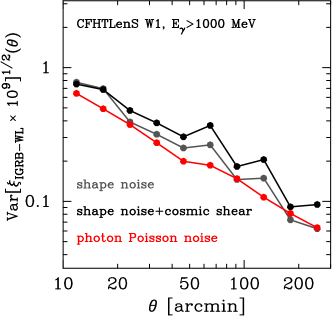
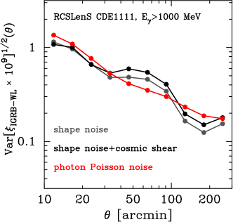
Figure 4 shows representative examples of the statistical uncertainty of our cross-correlation measurements. In both panels, we show the different contributions to the covariance of : the red line shows the covariance associated with the Poisson noise of photon counts ( and ); the gray line represents the covariance from intrinsic shape noise (expressed as ); and the black line is for the covariance associated with galaxy imaging surveys including the shape noise and the sample variance of cosmic shear (+). The left panel corresponds to the variance in the W1 field of CFHTLenS, while the right is for CDE1111 field of RCSLenS. Note that both covers a similar survey area, but the CFHTLenS field contains a factor more source galaxies. Figure 4 clearly shows that the sample variance of cosmic shear can be subdominant, but contributes at the level of to the statistical error on large angular scales of degrees. In the following, we therefore include all contributions of the covariance for completeness. The total covariance is estimated as the sum of the red and black lines in Figure 4.
IV.3 Systematic uncertainties
Diffuse Galactic rays are produced through the interactions of high-energy CR particles with interstellar gas via nucleon-nucleon inelastic collisions and electron Bremsstrahlung, and with the interstellar radiation field, via IC scattering. Such diffuse Galactic emission accounts for more than 60% of the photons detected by the Fermi-LAT. Modeling this component can thus introduce a large impact on the properties of the IGRB.
We estimated the systematic uncertainties in the DGB in a similar fashion to that in Ref. (Ackermann et al., 2012). We constructed eight different diffuse emission models using GALPROP (Strong et al., ) and each of these templates were included in the likelihood fit of the lensing surveys as an alternative to the standard DGB recommended in the 3FGL catalog (Acero et al., 2015).
The set of alternative DGB models taken into account in this analysis consider a range of possible values for the input parameters that were found to affect the most the -ray fits performed by the Fermi team in Ref. (Ackermann et al., 2012). The parameters varied in the models are the CR source distribution (supernova remnants or pulsars), CR halo heights (4 kpc or 10 kpc), and the atomic hydrogen spin temperature ( K or optically thin). In all of the GALPROP runs an magnitude cut of 5 mag was chosen. The impact in the resulting IGRB spectra obtained through this method is displayed as a green shaded area in Fig. 5.
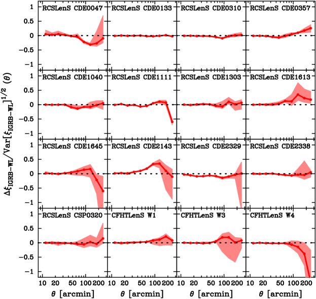
We use these eight model templates and repeat the cross-correlation analysis described in Sec. IV.1. We therefore obtain eight different binned signals () as functions of angular separation for each ROI. We introduce the following quantity for convenience,
| (24) | |||||
where is the cross-correlation signal measured with the IGRB intensity constructed by the fiducial Galactic templete, and is for the IGRB intensity with the GALPROP Galactic template.
Figure 6 summarizes the systematic effect associated with the subtraction of Galactic rays. In this figure, the red line shows the average over the eight different GALPROP templates, while the hatched region is for the scatter of . Note that the amplitudes are normalized by the statistical uncertainty evaluated in Sec. IV.2. The figure shows that our measurements are insensitive to the choice of Galactic -ray template, and that the typical systematic uncertainty in each ROI is smaller than the statistical uncertainty by a factor of . The small effect of the Galactic -ray template uncertainty is consistent with previous works Shirasaki et al. (2015b), and derives from the high latitudes of our ROIs; had we chosen ROIs closer to the Galactic plane, the model uncertainty would likely be significantly larger. Nevertheless, we also find that some ROIs show a relatively large difference among adopted Galactic templates at large angular separations (e.g., ). We have confirmed that our results remain robust when we limit the angular scale by where represents the statistical variance of our cross correlation measurements.
V RESULT
V.1 Cross-correlation measurement
Here we present the cross-correlation measurements of the IGRB and cosmic shear that we use to probe the parameter space of generic DM models.
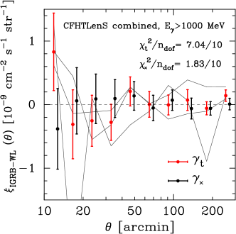
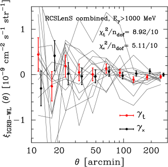
Figure 7 summarizes the cross-correlation signals obtained for the CFHTLenS and RCSLenS fields. The top panel shows the result obtained for CFHTLenS, while the bottom is for RCSLenS. In each panel, the gray thin line shows the cross-correlation signal estimated with Eq. (18) for each patch in the lensing survey. To combine the measured signal with different patches, we introduce the weighted cross-correlation signal over the different patches,
| (25) |
where represents the measured signal for the -th ROI and the summation is taken over all ROIs of interest. We determine the weight for a given by minimization of variance of . The minimum variance weight is then given by,
| (26) |
where represents the variance of and we assume that the cross covariance between different two patches can be ignored.
We then evaluate the significance of measured signals by using the signal-to-noise ratio for Eq. (25),
| (27) | |||||
| (28) |
where represents the covariance matrix for . The red point with error bar in Figure 7 shows the weighted signal for the tangential shear, while the black point with error bar is for the cross component of shear as an indicator of lensing systematics. We find that the cross-correlation signals in both CFHTLenS and RCSLenS are consistent with null detection. The resulting per number of degree of freedoms is for CFHTLenS and for RCSLenS. When combing all fields in CFHTLenS and RCSLenS, in Eq. (28) is 8.99. Also, we confirm that the for is consistent with null signal, suggesting the lensing systematics in our measurement are under control. We also define the significance for each ROI as
| (29) |
where we confirm that the is still consistent with null detection for a given -th ROI. Table 2 summarizes the results of our cross-correlation measurements.
| Survey | Name of patch | for | for |
|---|---|---|---|
| W1 | 2.40/10 | 4.13/10 | |
| W3 | 5.00/10 | 2.77/10 | |
| W4 | 10.45/10 | 6.46/10 | |
| CFHTLenS | 7.04/10 | 1.83/10 | |
| CDE0047 | 6.26/10 | 4.27/10 | |
| CDE0133 | 4.91/10 | 4.11/10 | |
| CDE0310 | 5.22/10 | 5.10/10 | |
| CDE0357 | 7.21/10 | 8.08/10 | |
| CDE1040 | 9.40/10 | 8.53/10 | |
| CDE1111 | 8.67/10 | 11.92/10 | |
| CDE1303 | 1.60/10 | 4.54/10 | |
| CDE1613 | 6.50/10 | 3.26/10 | |
| CDE1645 | 1.40/10 | 10.04/10 | |
| CDE2143 | 2.22/10 | 5.61/10 | |
| CDE2329 | 4.40/10 | 8.72/10 | |
| CDE2338 | 7.84/10 | 6.40/10 | |
| CSP0320 | 4.03/10 | 6.46/10 | |
| RCSLenS | 8.92/10 | 5.11/10 | |
| TOTAL | 8.99/10 | 3.74/10 |
V.2 Constraints on particle dark matter
In order to use the null detection of the cross-correlation to place constraints on particle DM, we use a maximum likelihood analysis. We assume that the data vector is well approximated by the multivariate Gaussian distribution with covariance . In this case, the statistics (log-likelihood) is given by,
| (30) |
where is the theoretical template for the set of parameters of interest. The theoretical prediction is computed as in Section II.3. The parameters of interest are the DM particle mass and the annihilation cross section for annihilating DM; as for decaying DM, we consider and the decay rate .
The data vector consists of the ten measured cross-correlation amplitudes in the range of arcmin as,
| (31) |
where is the -th angular separation bin. The inverse covariance matrix includes the statistical error owing to the intrinsic shape of galaxies, the sample variance of cosmic shear, and the photon Poisson error (see Section IV.2). In our likelihood analysis, we assume that the 16 patches of CFHTLenS and RCSLenS are independent of each other. With this assumption, the total log-likelihood is given by the sum of Eq. (30) in each patch of CFHTLenS and RCSLenS. We consider the 95% confidence level posterior distribution function of parameters. This is given by the contour line in the two dimensional space ( and , or and ), defined as
| (32) |
Note that the constraints in the following are based on all the measurements presented in this paper. Compared to the constraints using CFHTLenS alone Shirasaki et al. (2014), the present analysis combines CFHTLenS and RCSLenS, resulting in a factor of improvement. This derives from several factors, namely, (i) better -ray photon data quality and higher statistics, (ii) the increase in the number of source galaxies, and (iii) the use of large angular separations, i.e., arcmin. When we limit the angular range to arcmin, the constraints are degraded by a factor of , even if both CFHTLenS and RCSLenS are used. This indicates that the main cosmological information comes from large angular scales, making large sky coverage essential for maximizing the information content of our cross-correlation statistics. Note that our limit in this paper corresponds to the 95% confidence level, while our previous study using CFHTLenS in Ref Shirasaki et al. (2014) derived constraints based on the 68% confidence level.
Dark matter annihilation
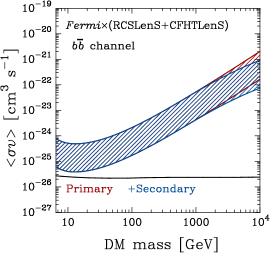
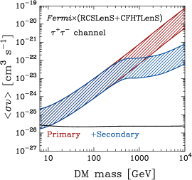
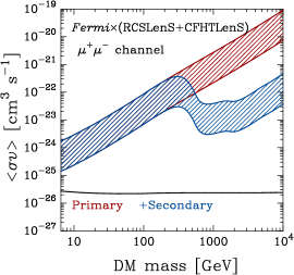
As discussed in Section II.3, the choice of the boost factor affects the theoretical predictions significantlyby a factor of . We therefore derive constraints based on both; an optimistic scenario as in Ref. Gao et al. (2012), and a conservative one following Ref. Sánchez-Conde and Prada (2014).
Figure 8 summarizes the constraints on DM annihilation with our cross-correlation measurements. These were obtained for three representative channels: , and . In Figure 8, the red line shows the constraints obtained by considering primary -ray emissions alone, while the blue line includes the secondary emission due to IC scattering between secondary and the CMB. As expected, heavier DM particles have a larger contribution of rays induced by the IC process. Thus, the constraints on heavier DM particles can be significantly improved when the secondary emission is taken into accountthe typical improvement is of order 100. Notice that leptonic channels are further enhanced by the secondary emission since more energetic tend to be produced. For very high DM masses , we find that the constraints are degraded by a factor of because the peak energy in is found to be outside our -ray energy range of 1-500 GeV.
Dark matter decay
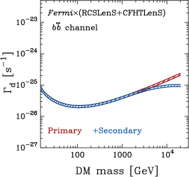
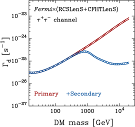
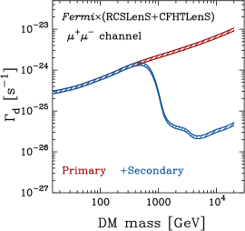
We next consider decaying DM. As discussed in Section II.3, the cross-correlation signal for DM decay can be predicted by the three-dimensional clustering of the DM density distribution. Conservatively, we consider two models of : one is based on the fitting formula of calibrated with a set of cosmological N-body simulations Takahashi et al. (2012), and the second one is an even more conservative scenario that uses only the linear matter power spectrum. Despite this rather extreme treatment of model uncertainty, we find that our results are fairly robust to the choice of the model of , introducing only some differences.
Our constraints on decaying DM are shown in Fig. 9. Similarly to the annihilating DM case, the constraints on the decay rate for heavy DM particles are improved by a factor of when secondary emission is accounted for. This trend is more prominent for the leptonic decay channels than the hadronic channel.
In part due to the accurate models of , the uncertainty from cosmic structure formation models in the DM decay constraint is significantly small compared to the uncertainty in DM annihilation. Although the resulting constraints are 10 times weaker than the recent constraints with the spectrum of IGRB intensity Ando and Ishiwata (2015) and the cross-correlation of the IGRB and local galaxy distributions Ando and Ishiwata (2016), they are the first constraints obtained from unbiased matter distributions outside the local Universe. Note that the previous constraints Ando and Ishiwata (2015, 2016) have been derived by the full-sky analysis of rays, while our constraints are based on the cross-correlation analysis with smaller sky fraction. When considering upcoming imaging surveys with a sky coverage of 20,000 squared degrees, we find that the expected constraints would be very similar to the constraints in the literature (see Section VI).
Wino dark matter
Finally, we explore the parameter space of particular wino DM models that are well motivated in particle physics. The wino DM is the lightest supersymmetric particle (LSP) of triplet Majorana fermion and realized in a wide range of supersymmetric standard models in which the anomaly mediation effect dominantly generates the gaugino masses Randall and Sundrum (1999); Giudice et al. (1998).
After the discovery of the Higgs boson with a mass of around 125 GeV Aad et al. (2012); Chatrchyan et al. (2012), models with the anomaly mediation and high-scale supersymmetry breaking is one of the most attractive candidates for physics beyond the standard model Hall and Nomura (2012); Hall et al. (2013); Ibe and Yanagida (2012); Ibe et al. (2012); Arvanitaki et al. (2013); Arkani-Hamed et al. (2012); Nomura and Shirai (2014), since this framework is compatible with the observed Higgs boson mass Okada et al. (1991a, b); Ellis et al. (1991a); Haber and Hempfling (1991); Ellis et al. (1991b), and predicts the wino LSP as a good DM candidate. The wino dark matter of a mass less than around 3 TeV is consistent with the observed DM abundance Hisano et al. (2007). The current LHC bound on the wino mass is around 270 GeV Aad et al. (2013); Khachatryan et al. (2015). At present there is no constraint on the wino DM from direct detection experiments and 10 ton class experiments may test the wino DM Hisano et al. (2010, 2013, 2015).
A prominent feature of the wino DM is considerably enhanced annihilation cross section by the Sommerfeld effects Hisano et al. (2004, 2005). Due to such a large annihilation cross section, indirect detection of the wino DM through cosmic-ray signals is promising. In fact, the -ray searches such as observation of the dwarf spheroidal galaxies by Fermi-LAT, and the galactic center by H.E.S.S. and antiproton searches by AMS-02 Cohen et al. (2013); Fan and Reece (2013); Hryczuk et al. (2014); Bhattacherjee et al. (2014); Ibe et al. (2015) can severely constrain the wino DM. These constraints may, however, suffer from potentially large systematic and astrophysical uncertainties such as the distribution of DM and that of other astrophysical sources. Therefore, it is important to examine the wino DM with our cross-correlation statistics, which has totally different systematics.
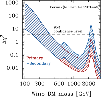
In order to derive constraints on the wino mass, we adopt the annihilation cross-section including the one-loop and Sommerfeld corrections Hryczuk and Iengo (2012). We assume that wino DM annihilates mainly into . The primary and secondary -ray emissions for channel are evaluated with PPPC4DMID package Cirelli et al. (2011) and the method shown in Ref. Ando and Ishiwata (2015, 2016).
Figure 10 shows the confidence level of wino DM model derived from our cross-correlation analysis. Note that the single parameter of wino mass is of interest in the case of wino DM model. In this figure, the red and blue lines represent as a function of wino mass in absence and presence of secondary emissions, respectively. The hatched regions show the model uncertainty of boost factor in our benchmark model (see Section II.3 in detail). Our result excludes the wino mass with GeV and (95% C.L.) in the case of the optimistic boost factor model and GeV in the conservative case. The constraint is already close to that derived by the LHC Aad et al. (2013) and can be further improved with ongoing and upcoming imaging surveys that cover a wider area than squared degrees considered here.
Note also that the secondary -ray emission originated from heavy DM particle tend to have lower energies. Thus, it would be possible to make the constraint tighter by using -ray photons with lower energy. On the other hand, the angular resolution becomes worse, or the photon noise increases when we use the low-energy rays. It would also be necessary to examine carefully systematic uncertainties associated with Galactic -ray emissions.
VI CONCLUSION AND DISCUSSION
We have performed cross-correlation analyses of the IGRB and cosmic shear using data from the Fermi-LAT and two galaxy imaging surveys, CFHTLenS and RCSLenS. Compared with our earlier study Shirasaki et al. (2014), the present study benefits not only from the increased survey area, but also from the following three aspects:
-
1.
The use of reprocessed -ray data with the Pass 8 pipeline.
The improved photon event characterization decreases the size of point spread function (PSF) in the energy range of 1 GeV to arcmin, allowing us to access the cross-correlation signals at small angular scales originating from -ray emission within single DM halos. The effective area is also increased, which when coupled with the improved PSF also allows an improved characterization of the IGRB.
-
2.
Reduction of the statistical uncertainty by using twelve million galaxies.
Our cross-correlation analysis is based on the ensemble average of galaxy-photon pairs. Hence the statistical uncertainty is largely determined by the number of galaxy-photon pairs. With about twelve million galaxies, we have reduced the statistical uncertainties by factor of compared to our previous study.
-
3.
An accurate model of the sample variance of cosmic shear.
Our cross-correlation measurement using 661 squared-degrees sky coverage is still consistent with null detection. With our accurate treatment on both statistical and systematic uncertainties, we fully utilized the cross-correlation measurement in the range of 10-300 arcmin, allowing us to improve the cosmological constraint by a factor of a few 555 If we adopted the Planck results Ade et al. (2015), we would have derived slightly tighter constraints because of the difference in and . We investigate a generic class of particle DM assuming three representative annihilation/decay channels. Because we include the contribution from secondary rays produced through inverse-Compton scattering of CMB photons, we are able to improve the DM constraints by a factor of for TeV-scale DM with leptonic channels.
Using GALPROP models, we have shown explicitly that the systematic uncertainties due to imperfect knowledge of Galactic -ray emission are unimportant compared to the statistical error in our measurement at present: we find that the typical systematic uncertainty is of the statistical error when using 12 million galaxies. This conclusion is consistent with the analysis of correlation with the spatial distribution of galaxies Shirasaki et al. (2015b). However, the uncertainty due to uncertain Galactic emission will likely become an issue in the future. First, future wide-area imaging surveys, such as the Large Synoptic Survey Telescope (LSST), will have a sky coverage of some 20,000 square degrees and source number density of 30 . We expect to use 2.16 billion galaxies in the cross-correlation measurement, improving potentially the statistical uncertainty by a factor of . Thus, the error on cross-correlation measurement would be dominated by systematic uncertainties due to the subtraction of Galactic -rays from the observed photon counts. Second, recent evidence for significant large-scale time-dependent contributions to the cosmic rays, e.g., the Fermi bubble Su et al. (2010), are starting to motivate studies beyond the stationary-state GALPROP treatment.
If we can reduce the statistical error to the level where the measurement is limited by the current systematic uncertainties, a wide range of annihilating DM models with a thermal cross section can be excluded: ( channels), ( channels), and ( channels). Such tight constraints can actually test various hints of DM signals reported so far. For example, the Galactic center excess Goodenough and Hooper (2009); Hooper and Goodenough (2011); Boyarsky et al. (2011); Hooper and Linden (2011); Abazajian and Kaplinghat (2012); Gordon and Macias (2013); Macias and Gordon (2014); Calore et al. (2015a, b); Abazajian et al. (2014); Daylan et al. (2016); Macias et al. (2015); Ajello et al. (2016); Lacroix et al. (2016); Horiuchi et al. (2016a), when interpreted as owing to DM annihilation, requires a cross section – over DM mass – GeV, depending on the precise annihilation channel. Moreover, in the specific model of wino DM, all the viable wino DM mass region ( TeV) can be tested in the case of the optimistic boost factor model. With the conservative assumption, the wino mass and may be excluded. Similarly, we find decaying DM models in the wide range of 10 GeV–20 TeV with ( channels), ( channels), and ( channels) are excluded when the measurement would be limited by the current systematic uncertainties. For specific DM models, these constraints can be further combined with constraints from additional probes such as direct detection and collider searches, e.g., (Horiuchi et al., 2016b).
We have shown that the cross-correlation analysis with the IGRB intensity and cosmic shear opens a new window to indirect detection of DM. Similar analysis using data from future surveys will provide competitive and independent constraints on the nature of DM from the local dwarf galaxy constraints. Remaining important issues include, (i) reducing the uncertainty due to Galactic -ray subtraction, (ii) direct measurement or constraints on the abundance of substructures within DM halos, (iii) optimization of detection of the cross-correlation signals between the IGRB intensity and cosmic shear, and (iv) joint analysis with Galactic and extragalactic measurements. There appear to be a few ways to increase the signal-to-noise ratio of the cross-correlation. For example, detection of DM halos in cosmic shear analyses Maturi et al. (2005); Hennawi and Spergel (2005) can help us with reconstructing the DM distribution more accurately. In the next decades, a wealth of astronomical survey data in multi-wavelengths will be steadily collected. Precise statistical analysis of such big data will shed light on the long-standing mystery of the nature of DM.
Acknowledgements.
M.S. is supported by Research Fellowships of the Japan Society for the Promotion of Science (JSPS) for Young Scientists. N.Y. acknowledges financial support from JST CREST. Numerical computations presented in this paper were in part carried out on the general-purpose PC farm at Center for Computational Astrophysics, CfCA, of National Astronomical Observatory of Japan. We thank the Fermi Collaboration for the use of Fermi public data and the Fermi Science Tools. This work is based on observations obtained with MegaPrime/MegaCam, a joint project of CFHT and CEA/IRFU, at the Canada-France-Hawaii Telescope (CFHT) which is operated by the National Research Council (NRC) of Canada, the Institut National des Sciences de l’Univers of the Centre National de la Recherche Scientifique (CNRS) of France, and the University of Hawaii. This research used the facilities of the Canadian Astronomy Data Centre operated by the National Research Council of Canada with the support of the Canadian Space Agency. In CFHTLenS and RCSLenS, data processing was made possible thanks to significant computing support from the NSERC Research Tools and Instruments grant program.References
- Hinshaw et al. (2013) G. Hinshaw et al. (WMAP), Astrophys. J. Suppl. 208, 19 (2013), arXiv:1212.5226 [astro-ph.CO] .
- Ade et al. (2014) P. A. R. Ade et al. (Planck), Astron. Astrophys. 571, A16 (2014), arXiv:1303.5076 [astro-ph.CO] .
- Eisenstein et al. (2005) D. J. Eisenstein et al. (SDSS), Astrophys. J. 633, 560 (2005), arXiv:astro-ph/0501171 [astro-ph] .
- Persic et al. (1996) M. Persic, P. Salucci, and F. Stel, Mon.Not.Roy.Astron.Soc. 281, 27 (1996), arXiv:astro-ph/9506004 [astro-ph] .
- Clowe et al. (2006) D. Clowe, M. Bradac, A. H. Gonzalez, M. Markevitch, S. W. Randall, C. Jones, and D. Zaritsky, Astrophys. J. 648, L109 (2006), arXiv:astro-ph/0608407 [astro-ph] .
- Bacon et al. (2000) D. J. Bacon, A. R. Refregier, and R. S. Ellis, Mon. Not. Roy. Astron. Soc. 318, 625 (2000), arXiv:astro-ph/0003008 [astro-ph] .
- Kilbinger et al. (2013) M. Kilbinger, L. Fu, C. Heymans, F. Simpson, J. Benjamin, et al., Mon.Not.Roy.Astron.Soc. 430, 2200 (2013), arXiv:1212.3338 [astro-ph.CO] .
- Becker et al. (2015) M. R. Becker et al. (DES), (2015), arXiv:1507.05598 [astro-ph.CO] .
- Jungman et al. (1996) G. Jungman, M. Kamionkowski, and K. Griest, Phys.Rept. 267, 195 (1996), hep-ph/9506380 .
- Funk (2015) S. Funk, (2015), arXiv:1508.05190 [astro-ph.HE] .
- Ajello et al. (2015) M. Ajello, D. Gasparrini, M. Sánchez-Conde, G. Zaharijas, M. Gustafsson, J. Cohen-Tanugi, C. D. Dermer, Y. Inoue, D. Hartmann, M. Ackermann, K. Bechtol, A. Franckowiak, A. Reimer, R. W. Romani, and A. W. Strong, Astrophys.J.Lett. 800, L27 (2015), arXiv:1501.05301 [astro-ph.HE] .
- Fornasa and Sánchez-Conde (2015) M. Fornasa and M. A. Sánchez-Conde, Phys. Rept. 598, 1 (2015), arXiv:1502.02866 [astro-ph.CO] .
- Camera et al. (2013) S. Camera, M. Fornasa, N. Fornengo, and M. Regis, Astrophys.J. 771, L5 (2013), arXiv:1212.5018 [astro-ph.CO] .
- Fornengo and Regis (2014) N. Fornengo and M. Regis, Frontiers in Physics 2, 6 (2014), arXiv:1312.4835 [astro-ph.CO] .
- Ando et al. (2014) S. Ando, A. Benoit-Lévy, and E. Komatsu, Phys.Rev. , 023514 (2014), arXiv:1312.4403 .
- Ando (2014) S. Ando, JCAP 1410, 061 (2014), arXiv:1407.8502 [astro-ph.CO] .
- Camera et al. (2015) S. Camera, M. Fornasa, N. Fornengo, and M. Regis, JCAP 6, 029 (2015), arXiv:1411.4651 .
- Xia et al. (2015) J.-Q. Xia, A. Cuoco, E. Branchini, and M. Viel, Astrophys.J.Suppl. 217, 15 (2015), arXiv:1503.05918 .
- Regis et al. (2015) M. Regis, J.-Q. Xia, A. Cuoco, E. Branchini, N. Fornengo, and M. Viel, Physical Review Letters 114, 241301 (2015), arXiv:1503.05922 .
- Cuoco et al. (2015) A. Cuoco, J.-Q. Xia, M. Regis, E. Branchini, N. Fornengo, and M. Viel, (2015), arXiv:1506.01030 [astro-ph.HE] .
- Shirasaki et al. (2014) M. Shirasaki, S. Horiuchi, and N. Yoshida, Phys.Rev. D90, 063502 (2014), arXiv:1404.5503 [astro-ph.CO] .
- Gilmore et al. (2012) R. Gilmore, R. Somerville, J. Primack, and A. Dominguez, Mon.Not.Roy.Astron.Soc. 422, 3189 (2012), arXiv:1104.0671 [astro-ph.CO] .
- Ishiwata et al. (2009) K. Ishiwata, S. Matsumoto, and T. Moroi, Phys. Lett. B679, 1 (2009), arXiv:0905.4593 [astro-ph.CO] .
- Brunetti and Jones (2014) G. Brunetti and T. W. Jones, International Journal of Modern Physics D 23, 1430007-98 (2014), arXiv:1401.7519 .
- Bartelmann and Schneider (2001) M. Bartelmann and P. Schneider, Phys.Rept. 340, 291 (2001), arXiv:astro-ph/9912508 [astro-ph] .
- Cirelli et al. (2011) M. Cirelli, G. Corcella, A. Hektor, G. Hutsi, M. Kadastik, P. Panci, M. Raidal, F. Sala, and A. Strumia, JCAP 1103, 051 (2011), [Erratum: JCAP1210,E01(2012)], arXiv:1012.4515 [hep-ph] .
- Ando and Ishiwata (2015) S. Ando and K. Ishiwata, JCAP 1505, 024 (2015), arXiv:1502.02007 [astro-ph.CO] .
- Ando and Ishiwata (2016) S. Ando and K. Ishiwata, (2016), arXiv:1604.02263 [hep-ph] .
- Limber (1954) D. N. Limber, Astrophys.J. 119, 655 (1954).
- de Putter and Takada (2010) R. de Putter and M. Takada, Phys.Rev. D82, 103522 (2010), arXiv:1007.4809 [astro-ph.CO] .
- Oguri and Takada (2011) M. Oguri and M. Takada, Phys.Rev. D83, 023008 (2011), arXiv:1010.0744 [astro-ph.CO] .
- Cooray and Sheth (2002) A. Cooray and R. K. Sheth, Phys.Rept. 372, 1 (2002), arXiv:astro-ph/0206508 [astro-ph] .
- Tinker et al. (2008) J. L. Tinker, A. V. Kravtsov, A. Klypin, K. Abazajian, M. S. Warren, et al., Astrophys.J. 688, 709 (2008), arXiv:0803.2706 [astro-ph] .
- Tinker et al. (2010) J. L. Tinker, B. E. Robertson, A. V. Kravtsov, A. Klypin, M. S. Warren, et al., Astrophys.J. 724, 878 (2010), arXiv:1001.3162 [astro-ph.CO] .
- Navarro et al. (1997) J. F. Navarro, C. S. Frenk, and S. D. White, Astrophys.J. 490, 493 (1997), arXiv:astro-ph/9611107 [astro-ph] .
- Prada et al. (2012) F. Prada, A. A. Klypin, A. J. Cuesta, J. E. Betancort-Rijo, and J. Primack, Mon. Not. Roy. Astron. Soc. 428, 3018 (2012), arXiv:1104.5130 [astro-ph.CO] .
- Gao et al. (2012) L. Gao, C. Frenk, A. Jenkins, V. Springel, and S. White, Mon.Not.Roy.Astron.Soc. 419, 1721 (2012), arXiv:1107.1916 [astro-ph.CO] .
- Sánchez-Conde and Prada (2014) M. A. Sánchez-Conde and F. Prada, Mon. Not. Roy. Astron. Soc. 442, 2271 (2014), arXiv:1312.1729 [astro-ph.CO] .
- Bartels and Ando (2015) R. Bartels and S. Ando, Phys. Rev. D92, 123508 (2015), arXiv:1507.08656 [astro-ph.CO] .
- Atwood et al. (2009) W. B. Atwood, A. A. Abdo, M. Ackermann, W. Althouse, B. Anderson, M. Axelsson, L. Baldini, J. Ballet, D. L. Band, G. Barbiellini, and et al., Astrophys. J. 697, 1071 (2009), arXiv:0902.1089 [astro-ph.IM] .
- Takahashi et al. (2012) R. Takahashi, M. Sato, T. Nishimichi, A. Taruya, and M. Oguri, Astrophys. J. 761, 152 (2012), arXiv:1208.2701 [astro-ph.CO] .
- Note (1) ULTRACLEANVETO events are the recommended class of photons for investigation of the IGRB at intermediate to high latitudes. The reader is referred to the Cicerone (%****␣ms.bbl␣Line␣575␣****http://fermi.gsfc.nasa.gov/ssc/data/analysis/documentation/Pass8_usage.html) for further details.
- Acero et al. (2015) F. Acero, M. Ackermann, M. Ajello, A. Albert, et al. (Fermi-LAT), Astrophys.J.Suppl. 218, 23 (2015), arXiv:1501.02003 [astro-ph.HE] .
- Note (2) http://fermi.gsfc.nasa.gov/ssc/data/analysis/documentation/.
- Note (3) Http://fermi.gsfc.nasa.gov/ssc/data/analysis/.
- Note (4) http://fermi.gsfc.nasa.gov/ssc/data/analysis/scitools/solar_template.html.
- Macias and Gordon (2014) O. Macias and C. Gordon, Phys. Rev. D89, 063515 (2014), arXiv:1312.6671 [astro-ph.HE] .
- Abazajian et al. (2014) K. N. Abazajian, N. Canac, S. Horiuchi, and M. Kaplinghat, Phys. Rev. D90, 023526 (2014), arXiv:1402.4090 [astro-ph.HE] .
- Ackermann et al. (2015) M. Ackermann et al. (Fermi-LAT), Astrophys. J. 799, 86 (2015), arXiv:1410.3696 [astro-ph.HE] .
- Heymans et al. (2012) C. Heymans, L. Van Waerbeke, L. Miller, T. Erben, H. Hildebrandt, et al., Mon.Not.Roy.Astron.Soc. 427, 146 (2012), arXiv:1210.0032 [astro-ph.CO] .
- Hildebrandt et al. (2016) H. Hildebrandt et al., (2016), arXiv:1603.07722 [astro-ph.CO] .
- Harnois-Déraps et al. (2016) J. Harnois-Déraps et al., (2016), 10.1093/mnras/stw947, arXiv:1603.07723 [astro-ph.CO] .
- Hildebrandt et al. (2012) H. Hildebrandt, T. Erben, K. Kuijken, L. van Waerbeke, C. Heymans, et al., Mon.Not.Roy.Astron.Soc. 421, 2355 (2012), arXiv:1111.4434 [astro-ph.CO] .
- Erben et al. (2013) T. Erben, H. Hildebrandt, L. Miller, L. van Waerbeke, C. Heymans, et al., Mon.Not.Roy.Astron.Soc. 433, 2545 (2013), arXiv:1210.8156 [astro-ph.CO] .
- Miller et al. (2013) L. Miller, C. Heymans, T. Kitching, L. Van Waerbeke, T. Erben, et al., Mon.Not.Roy.Astron.Soc. 429, 2858 (2013), arXiv:1210.8201 [astro-ph.CO] .
- Benjamin et al. (2013) J. Benjamin, L. Van Waerbeke, C. Heymans, M. Kilbinger, T. Erben, et al., Mon.Not.Roy.Astron.Soc. 431, 1547 (2013), arXiv:1212.3327 [astro-ph.CO] .
- Benitez (2000) N. Benitez, Astrophys.J. 536, 571 (2000), arXiv:astro-ph/9811189 [astro-ph] .
- Gilbank et al. (2011) D. G. Gilbank, M. D. Gladders, H. K. C. Yee, and B. C. Hsieh, Astron. J. 141, 94 (2011), arXiv:1012.3470 [astro-ph.CO] .
- Coupon et al. (2015) J. Coupon et al., Mon. Not. Roy. Astron. Soc. 449, 1352 (2015), arXiv:1502.02867 [astro-ph.CO] .
- Shirasaki and Yoshida (2014) M. Shirasaki and N. Yoshida, Astrophys.J. 786, 43 (2014), arXiv:1312.5032 [astro-ph.CO] .
- Shirasaki et al. (2015a) M. Shirasaki, T. Hamana, and N. Yoshida, Mon. Not. Roy. Astron. Soc. 453, 3043 (2015a), arXiv:1504.05672 [astro-ph.CO] .
- Ackermann et al. (2012) M. Ackermann et al., The Astrophysical Journal 750, 3 (2012).
- (63) A. W. Strong et al., “Galprop version 54: Explanatory supplement,” http://galprop.stanford.edu, accessed: 2014-02-20.
- Shirasaki et al. (2015b) M. Shirasaki, S. Horiuchi, and N. Yoshida, Phys. Rev. D92, 123540 (2015b), arXiv:1511.07092 [astro-ph.CO] .
- Steigman et al. (2012) G. Steigman, B. Dasgupta, and J. F. Beacom, Phys. Rev. D 86, 023506 (2012), arXiv:1204.3622 [hep-ph] .
- Hryczuk and Iengo (2012) A. Hryczuk and R. Iengo, JHEP 01, 163 (2012), [Erratum: JHEP06,137(2012)], arXiv:1111.2916 [hep-ph] .
- Randall and Sundrum (1999) L. Randall and R. Sundrum, Nucl. Phys. B557, 79 (1999), arXiv:hep-th/9810155 [hep-th] .
- Giudice et al. (1998) G. F. Giudice, M. A. Luty, H. Murayama, and R. Rattazzi, JHEP 12, 027 (1998), arXiv:hep-ph/9810442 [hep-ph] .
- Aad et al. (2012) G. Aad et al. (ATLAS), Phys. Lett. B716, 1 (2012), arXiv:1207.7214 [hep-ex] .
- Chatrchyan et al. (2012) S. Chatrchyan et al. (CMS), Phys. Lett. B716, 30 (2012), arXiv:1207.7235 [hep-ex] .
- Hall and Nomura (2012) L. J. Hall and Y. Nomura, JHEP 01, 082 (2012), arXiv:1111.4519 [hep-ph] .
- Hall et al. (2013) L. J. Hall, Y. Nomura, and S. Shirai, JHEP 01, 036 (2013), arXiv:1210.2395 [hep-ph] .
- Ibe and Yanagida (2012) M. Ibe and T. T. Yanagida, Phys. Lett. B709, 374 (2012), arXiv:1112.2462 [hep-ph] .
- Ibe et al. (2012) M. Ibe, S. Matsumoto, and T. T. Yanagida, Phys. Rev. D85, 095011 (2012), arXiv:1202.2253 [hep-ph] .
- Arvanitaki et al. (2013) A. Arvanitaki, N. Craig, S. Dimopoulos, and G. Villadoro, JHEP 02, 126 (2013), arXiv:1210.0555 [hep-ph] .
- Arkani-Hamed et al. (2012) N. Arkani-Hamed, A. Gupta, D. E. Kaplan, N. Weiner, and T. Zorawski, (2012), arXiv:1212.6971 [hep-ph] .
- Nomura and Shirai (2014) Y. Nomura and S. Shirai, Phys. Rev. Lett. 113, 111801 (2014), arXiv:1407.3785 [hep-ph] .
- Okada et al. (1991a) Y. Okada, M. Yamaguchi, and T. Yanagida, Prog. Theor. Phys. 85, 1 (1991a).
- Okada et al. (1991b) Y. Okada, M. Yamaguchi, and T. Yanagida, Phys. Lett. B262, 54 (1991b).
- Ellis et al. (1991a) J. R. Ellis, G. Ridolfi, and F. Zwirner, Phys. Lett. B257, 83 (1991a).
- Haber and Hempfling (1991) H. E. Haber and R. Hempfling, Phys. Rev. Lett. 66, 1815 (1991).
- Ellis et al. (1991b) J. R. Ellis, G. Ridolfi, and F. Zwirner, Phys. Lett. B262, 477 (1991b).
- Hisano et al. (2007) J. Hisano, S. Matsumoto, M. Nagai, O. Saito, and M. Senami, Phys. Lett. B646, 34 (2007), arXiv:hep-ph/0610249 [hep-ph] .
- Aad et al. (2013) G. Aad et al. (ATLAS), Phys. Rev. D88, 112006 (2013), arXiv:1310.3675 [hep-ex] .
- Khachatryan et al. (2015) V. Khachatryan et al. (CMS), JHEP 01, 096 (2015), arXiv:1411.6006 [hep-ex] .
- Hisano et al. (2010) J. Hisano, K. Ishiwata, and N. Nagata, Phys. Lett. B690, 311 (2010), arXiv:1004.4090 [hep-ph] .
- Hisano et al. (2013) J. Hisano, K. Ishiwata, and N. Nagata, Phys. Rev. D87, 035020 (2013), arXiv:1210.5985 [hep-ph] .
- Hisano et al. (2015) J. Hisano, K. Ishiwata, and N. Nagata, JHEP 06, 097 (2015), arXiv:1504.00915 [hep-ph] .
- Hisano et al. (2004) J. Hisano, S. Matsumoto, and M. M. Nojiri, Phys. Rev. Lett. 92, 031303 (2004), arXiv:hep-ph/0307216 [hep-ph] .
- Hisano et al. (2005) J. Hisano, S. Matsumoto, M. M. Nojiri, and O. Saito, Phys. Rev. D71, 063528 (2005), arXiv:hep-ph/0412403 [hep-ph] .
- Cohen et al. (2013) T. Cohen, M. Lisanti, A. Pierce, and T. R. Slatyer, JCAP 1310, 061 (2013), arXiv:1307.4082 .
- Fan and Reece (2013) J. Fan and M. Reece, JHEP 10, 124 (2013), arXiv:1307.4400 [hep-ph] .
- Hryczuk et al. (2014) A. Hryczuk, I. Cholis, R. Iengo, M. Tavakoli, and P. Ullio, JCAP 1407, 031 (2014), arXiv:1401.6212 [astro-ph.HE] .
- Bhattacherjee et al. (2014) B. Bhattacherjee, M. Ibe, K. Ichikawa, S. Matsumoto, and K. Nishiyama, JHEP 07, 080 (2014), arXiv:1405.4914 [hep-ph] .
- Ibe et al. (2015) M. Ibe, S. Matsumoto, S. Shirai, and T. T. Yanagida, Phys. Rev. D91, 111701 (2015), arXiv:1504.05554 [hep-ph] .
- Note (5) If we adopted the Planck results Ade et al. (2015), we would have derived slightly tighter constraints because of the difference in and .
- Su et al. (2010) M. Su, T. R. Slatyer, and D. P. Finkbeiner, Astrophys. J. 724, 1044 (2010), arXiv:1005.5480 [astro-ph.HE] .
- Goodenough and Hooper (2009) L. Goodenough and D. Hooper, (2009), arXiv:0910.2998 [hep-ph] .
- Hooper and Goodenough (2011) D. Hooper and L. Goodenough, Phys.Lett. B697, 412 (2011), arXiv:1010.2752 [hep-ph] .
- Boyarsky et al. (2011) A. Boyarsky, D. Malyshev, and O. Ruchayskiy, Phys.Lett. B705, 165 (2011), arXiv:1012.5839 [hep-ph] .
- Hooper and Linden (2011) D. Hooper and T. Linden, Phys.Rev. D84, 123005 (2011), arXiv:1110.0006 [astro-ph.HE] .
- Abazajian and Kaplinghat (2012) K. N. Abazajian and M. Kaplinghat, Phys.Rev. D86, 083511 (2012), arXiv:1207.6047 [astro-ph.HE] .
- Gordon and Macias (2013) C. Gordon and O. Macias, Phys.Rev. D88, 083521 (2013), arXiv:1306.5725 [astro-ph.HE] .
- Calore et al. (2015a) F. Calore, I. Cholis, C. McCabe, and C. Weniger, Phys. Rev. D91, 063003 (2015a), arXiv:1411.4647 [hep-ph] .
- Calore et al. (2015b) F. Calore, I. Cholis, and C. Weniger, JCAP 1503, 038 (2015b), arXiv:1409.0042 [astro-ph.CO] .
- Daylan et al. (2016) T. Daylan, D. P. Finkbeiner, D. Hooper, T. Linden, S. K. N. Portillo, N. L. Rodd, and T. R. Slatyer, Phys. Dark Univ. 12, 1 (2016), arXiv:1402.6703 [astro-ph.HE] .
- Macias et al. (2015) O. Macias, R. Crocker, C. Gordon, and S. Profumo, Mon. Not. Roy. Astron. Soc. 451, 1833 (2015), arXiv:1410.1678 [astro-ph.HE] .
- Ajello et al. (2016) M. Ajello et al. (Fermi-LAT), Astrophys. J. 819, 44 (2016), arXiv:1511.02938 [astro-ph.HE] .
- Lacroix et al. (2016) T. Lacroix, O. Macias, C. Gordon, P. Panci, C. Bœhm, and J. Silk, Phys. Rev. D93, 103004 (2016), arXiv:1512.01846 [astro-ph.HE] .
- Horiuchi et al. (2016a) S. Horiuchi, M. Kaplinghat, and A. Kwa, (2016a), arXiv:1604.01402 [astro-ph.HE] .
- Horiuchi et al. (2016b) S. Horiuchi, O. Macias, D. Restrepo, A. Rivera, O. Zapata, and H. Silverwood, JCAP 1603, 048 (2016b), arXiv:1602.04788 [hep-ph] .
- Maturi et al. (2005) M. Maturi, M. Meneghetti, M. Bartelmann, K. Dolag, and L. Moscardini, Astron. Astrophys. 442, 851 (2005), arXiv:astro-ph/0412604 [astro-ph] .
- Hennawi and Spergel (2005) J. F. Hennawi and D. N. Spergel, Astrophys. J. 624, 59 (2005), arXiv:astro-ph/0404349 [astro-ph] .
- Ade et al. (2015) P. A. R. Ade et al. (Planck), (2015), arXiv:1502.01589 [astro-ph.CO] .