First Constraints on the Complete Neutrino Mixing Matrix with a Sterile Neutrino
Abstract
Neutrino oscillation models involving one extra mass eigenstate beyond the standard three () are fit to global short baseline experimental data and the recent IceCube disappearance search result. We find a best fit of with (dof) of 50.61 (4). We find that the combined IceCube and short baseline data constrain to at 90% C.L. for , which is improved over present limits. Incorporating the IceCube information provides the first constraints on all entries of the 3+1 mixing matrix.
pacs:
14.60.Pq,14.60.StI Introduction
Neutrino oscillations are due to quantum-mechanical effects that occur if the neutrino mass eigenstates are mixtures of the neutrino flavor eigenstates. These effects have been observed in multiple experiments [1]. Most neutrino oscillation data sets fit well into a model involving three active neutrinos that map to three distinct mass states through a unitary mixing matrix [1]. This three-neutrino model, then, has two independent squared-mass splittings, . The frequency of vacuum neutrino oscillations depends upon the magnitude of these squared-mass splittings. The larger of the two well-confirmed splittings, historically called the atmospheric splitting, is [2], while the smaller well-confirmed splitting, called the solar splitting, is [2].
On the other hand, a set of anomalous experiments provide indications of oscillations with substantially different frequency than the solar and atmospheric results. Results from LSND [3], MiniBooNE [4, 5], reactor experiments [6, 7], and Gallium source experiments [8, 9] are consistent with a third mass splitting, eV2. These experiments are generally classified as “short baseline” (SBL), meaning that they are designed with a distance-to-energy ratio for the neutrino source and detector of around . LSND and MiniBooNE observed electron flavor neutrino appearance in a muon-flavored beam. The reactor and source experiments observed electron-flavor disappearance. The significance of these signals ranges from 2 to 4, and hence are less compelling individually than the solar and atmospheric results. However, taken together, the results point to a new oscillation parameter region. To accommodate a third squared-mass splitting that is not the sum of the atmospheric and solar splittings, one must introduce a fourth neutrino mass state into the model. Since LEP Z0 decay measurements are consistent with only three low mass, active neutrinos [10], an additional fourth neutrino flavor must be inactive and is historically called sterile.
However, other SBL experiments sensitive to this higher oscillation frequency have observed null results [11, 12, 13, 14, 15, 16, 17, 18, 19, 20]. In particular, muon flavor disappearance has not been observed in SBL experiments. These limits must also be accounted for in any model with extra neutrino flavors. As a result, global fits of data employing three active neutrinos and one sterile neutrino, called 3+1 models, have a limited allowed range in vacuum oscillation parameter space [21, 22, 23]. Nevertheless, 3+1 models that fit all of the data sets do remain and have prompted a suite of new SBL experiments, which are now underway [24] or are in design [25, 26, 27, 28].
In Ref. [21], we have reported the results of global fits to the SBL data that yield allowed regions at 90% CL at three values at approximately 1, 1.75 and 6 eV2. In this paper, we expand these 3+1 fits to include a new, highly restrictive oscillation limit from the IceCube Experiment [29]. Because the IceCube analysis relies on matter effects rather than vacuum oscillations, this new data set breaks degeneracies, allowing, for the first time, to fill in all of the elements of the 3+1 mixing matrix.
II Constraints from SBL Experiments
SBL experiments have direct sensitivity to neutrino oscillations involving electron and muon flavor neutrinos, but do not have direct sensitivity to transitions involving the tau neutrino flavor. This is because the threshold for charged current interactions of 3.4 GeV suppresses charged current interactions for these low energy SBL experiments. A full 3+1 model, however, has a matrix that connects all three active plus single sterile flavor states to the four mass states:
| (1) |
Due the high production threshold, the SBL experiments can only directly constrain the elements and .
The observed anomalous mass splitting associated with oscillations to the fourth neutrino flavor is very large compared to the solar and atmospheric cases. Thus, for these oscillations, one can make the approximations that and . This leads to the SBL approximation for the vacuum oscillation probability formula for :
| (2) |
In this equation, is the distance the neutrino travels and is the energy of the neutrino. For a given choice of flavors and , this is equivalent to a two neutrino model with a mixing amplitude of
| (3) |
Thus, in this notation, muon-to-electron flavor appearance experiments measure , and the disappearance experiments measure and .
This paper makes use of the global fits to SBL data reported in Ref. [21]. The experiments are chosen to be relevant in the range of eV2 at 90% CL, which is the limit of LSND [3]. We fit in the range of eV2. The specifics of the SBL data sets are given in Table 1 of Ref. [21], and the associated text, and so we very briefly explain the choices here. With respect to electron neutrino appearance, we include LSND [3], MiniBooNE ( and from the BNB flux) [5, 30, 31, 4], MiniBooNE (NuMI off-axis flux) [32], KARMEN [11] and NOMAD[16]. With respect to electron neutrino disappearance, we include Bugey [6], the Gallium Experiments [8, 9] and the Karmen/LSND cross section analysis [12]. With respect to disappearance, we include the MiniBooNE-SciBooNE joint analyses in and running [33, 34], the CDHS result [18], MINOS results from 2006 and 2008 [19, 35] that are strictly from charged current analysis, and CCFR84 [17].
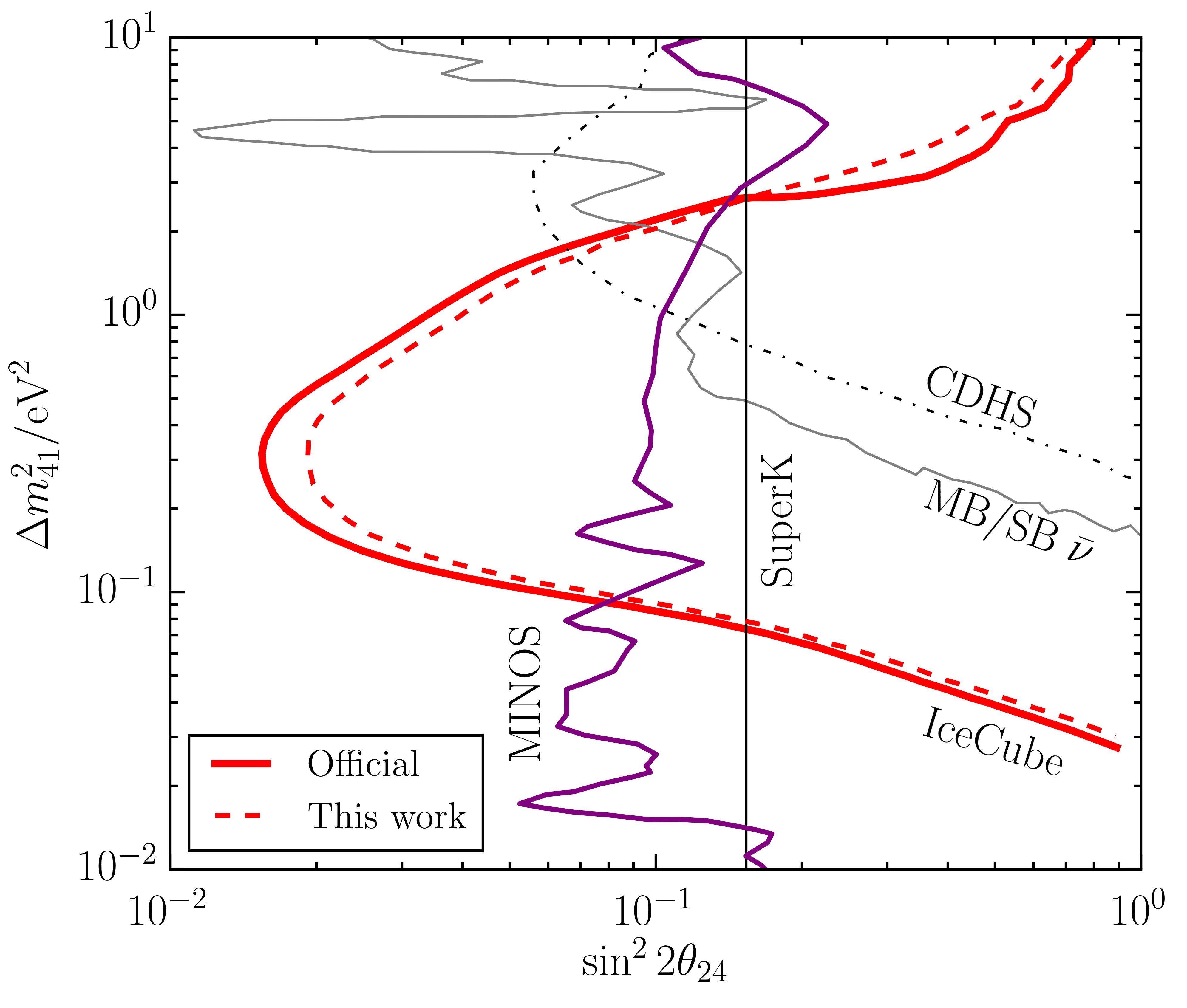
There are two results published in 2016 that are not included in these fits. The 2016 Daya Bay disappearance result, which is published for eV2 [36], need not be included in these fits. The small overlap is in a region dominated by the Bugey result already used in the fit [6]. The 2016 MINOS disappearance result [37] is not included in the fit for two reasons. First, this result is not competitive with the IceCube result and other data sets already used in the region of interest for the fits, as can be seen in Fig. 1. Second, this disappearance result incorporates neutral current data, with a background subtraction for the relatively large [38] intrinsic flux. Thus the MINOS limit is dependent on their assumption that and cannot be directly used in our global fits that need to include disappearance in an unrestricted way.
These fits also do not include data from cosmology because the CMB and large scale structure (LSS) constraints on the presence of a fourth neutrino are model dependent. The dependencies include assuming a “standard” thermal history for the Universe [39]. Sterile neutrino thermalization can be suppressed a number of plausible ways [40, 41, 42, 43, 44, 45, 46, 47, 48]. In fact, thermalization may not occur when one considers models with full four-neutrino mixing [49]. Introducing the assumption that sterile neutrinos have very weak pseudoscalar interactions that are unobservable in the short baseline data not only resolves the apparent disagreement between the 3+1 models and CMB, it also predicts a Hubble constant in agreement with local measurements [50]. Changes in the assumption of the influence of dark energy on the expansion history and growth structure also influences the comological results [39]. Based on this, rather than include cosmology in the fit, what is most interesting is to fit the cosmological data separately from the oscillation experiments, and then consider the meaning of discrepancies.
The global fit favors a model with one mass state dominated by the sterile flavor. The three assumed degenerate mass states are dominated by the active flavors, as is demanded by the solar and atmospheric neutrino results. The SBL fits cannot distinguish the mass hierarchy, that is, whether the dominantly sterile flavor is the highest mass state, which is called a 3+1 hierarchy, or the lowest mass state, which is called a 1+3 hierarchy.
III Incorporating IceCube Data
In this paper, we expand the 3+1 fits to include data from IceCube [29], which is quite different in design from the SBL experiments. It makes use of measurements of the atmospheric flux, studied as a function of the zenith angle and energy in the range from 400 GeV to 20 TeV. The detector consists of 86 strings of optical modules located within the Antarctic ice near the South Pole. The energy and path-length through the Earth of these atmospheric neutrinos is equivalent to an m/MeV value, similar to the SBL experiments. However, the strength of the IceCube null result, shown in Fig. 1, arises from the additional modifications of the oscillation behavior when high energy neutrinos travel through dense matter, called “matter effects.”
The matter-effect signature in IceCube corresponds to a predicted large deficit in the antineutrino flux for the up-going neutrinos that cross the Earth, given a 3+1 model with an anomalous squared mass splitting of eV2 [51, 52, 53, 54, 55, 56, 57]. This modification to the vacuum oscillation formalism comes from differences between neutrino charged- and neutral-current interactions with the earth. In experiments at low energy or short baselines, this effect is negligible, and only vacuum oscillations need to be considered. However, at the high energies and long baselines available to the IceCube experiment, coherent forward scattering can significantly affect neutrino propagation. In a 3+1 model, an additional matter potential is introduced to account for the difference of active flavor neutrinos scattering from matter–a contribution that is missing for the sterile flavor.
The matter effect is dependent on the neutrino mass hierarchy. In the case of a hierarchy, as opposed to a hierarchy, the matter-induced resonance will appear in the antineutrino events rather than the neutrino events. Detectable effects will lie in the range 0.01 eV2—the region of interest for our global fits. This follows from the the resonant energy: , where is an effective two flavor active-to-sterile neutrino mixing angle and is the target number density. The quoted sensitivity range can be understood by replacing by the corresponding density of the Earth, and the energy by the energy thresholds of the data set. It should be noted that the IceCube null result leads to a more restrictive limit in the case of 1+3 compared to a 3+1 model. This comes about because about 70% of the events in IceCube are due to neutrino interactions, where a 1+3 signal would appear. This is in agreement with the conclusions of cosmology and further justifies our concentration on 3+1 models below.
Use of matter effects in the IceCube analysis breaks degeneracies in the fits, allowing, for the first time, to constrain all of the elements of the 3+1 mixing matrix. Examining Eq. 1, one sees that the matrix has elements determined by the atmospheric and solar oscillation measurements, for which we use the results of Ref. [58] as the range of allowed values. This leaves seven further elements. Four of these elements, (), cannot be directly constrained by experiment due to the non-interacting nature of the ‘sterile’ flavor state. However, in a 3+1 model, the mixing matrix is unitary, and so these unmeasureable elements can be determined if the remaining three matrix elements are constrained. This leaves the elements , and to be determined from the global fits to the combined SBL and IceCube data sets that we present below.
The SBL approximation, which has been applied in our previous fits [21], cannot be applied when including the matter-effect signature in IceCube. In our global analysis, the SM values of and from Ref. [2] are used for and , respectively. Furthermore, the introduction of IceCube data requires a parameterization of the extended lepton mixing matrix, Eq. 1. This can be presented as a product of rotations following the convention specified in Ref. [59]:
| (4) |
Each is a rotation matrix through angle in the plane. In this parameterization, the fourth column of is given by
| (5) |
If one sets all the CP violating phases to zero, only three new angles are introduced: , , and . In addition, the IceCube collaboration analysis assumes . Under these assumptions, —the vacuum disappearance amplitude. While this is a convenient way to express the disappearance result (and is used in Ref. [29] along with other papers), these assumptions will need to be relaxed in order to include IceCube in the global fits.
| 3+1 | (dof) | |||||||
|---|---|---|---|---|---|---|---|---|
| SBL | 1.75 | 0.163 | 0.117 | - | 315 | 306.81 | 359.15 | 52.34 (3) |
| SBL+IC | 1.75 | 0.164 | 0.119 | 0.00 | 524 | 518.23 | 568.84 | 50.61 (4) |
| IC | 5.62 | - | 0.314 | - | 209 | 207.11 | 209.69 | 2.58 (2) |
| 6 | [0.17,0.21] | [0.10,0.13] | [0.00,0.05] | |
| 2 | [0.13,0.20] | [0.09,0.15] | [0.00,0.70] |
The IceCube analysis and the results presented here make use of the software package called nuSQuIDS [59, 60]. This software models flavor evolution from three (i.e. SM) to six flavor basis states with customized matter potentials. The 3+1 nuSQuIDS calculation does not use the short baseline approximation; thus, it includes the two additional violating parameters that arise when and are nonzero and not equal. However, in the case of the IceCube analysis, these parameters are set to zero. For the matter potential, nuSQuIDS makes use of the Preliminary Reference Earth Model (PREM) [61] parameterization describing the radial density profile of the Earth. The neutrino propagation implementation follows Eqs. (29-30) in Ref. [62]. For the neutrino nucleon cross sections, we use the perturbative QCD calculation from Ref. [63, 64].
No evidence for anomalous or disappearance was observed in the IceCube data set. The resulting stringent limit extends to 0.02 at 0.3 at 90% CL for [29]. To incorporate this result into the fit, we must relate the mixing angles , , and to the short-baseline neutrino oscillation probabilities. The oscillation amplitudes in this parameterization are found by substituting the matrix elements in Eq. (5) into Eq. (2); e.g., . Since the short baseline anomalies imply , it follows that we cannot assume in a global fit.
It has been shown [65] that the presence of the matter-induced resonance critically depends on the value of . In particular, when is maximal, there is no matter-induced resonant enhancement. On the other hand, as noted by Ref. [54], increasing distorts the atmospheric to neutrino oscillation. The interplay between these effects makes the IceCube data sensitive to . We obtain the constraint on this parameter by sampling logarithmically in from to 1. The phases have a sub-leading contribution in comparison to the effect [54]; thus, they have been set to zero.
We describe the specific techniques of including the IceCube data into the fits in the appendix to this article. Our capability of reproducing the IceCube result using the data release is shown in Fig. 1, dashed. The IceCube likelihood must be converted to a that can be combined with the SBL data. The high computational cost of propagating neutrino fluxes through the Earth with nuSQuIDS prevents the analysis from being directly included into the global fitting software. Instead, the global fits were used to find a reduced set of parameters (“test points”) that could be evaluated directly. This assumes that the effect of IceCube on the global fit is a small perturbation, which is reasonable given that the IceCube-only is small compared to the SBL only global fit (see Table 1).
IV Results
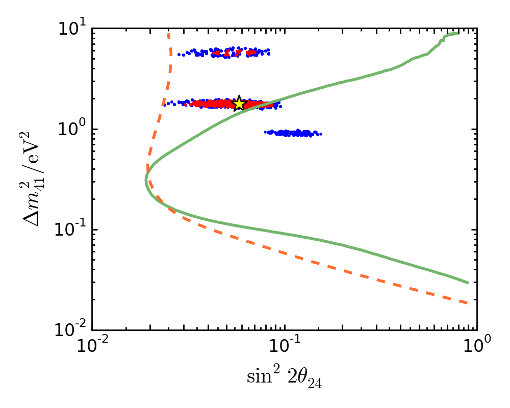
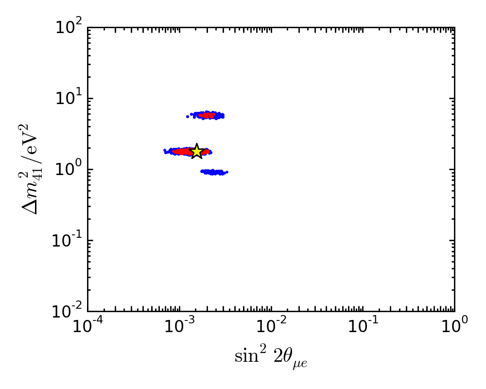
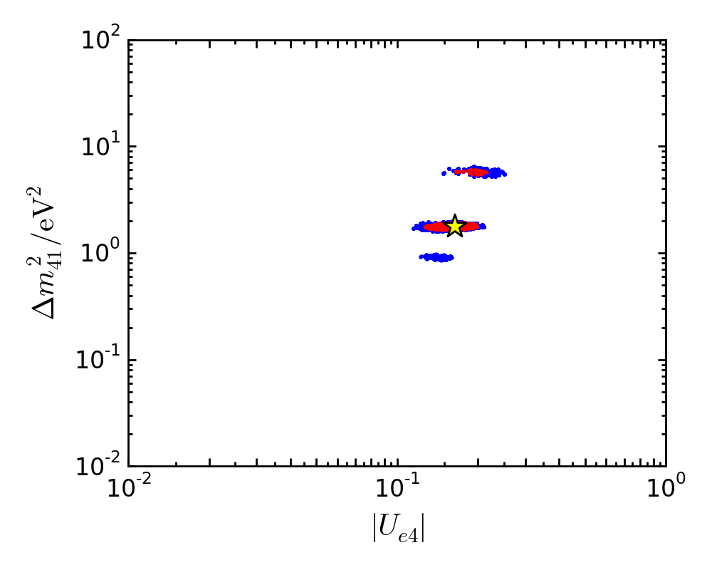
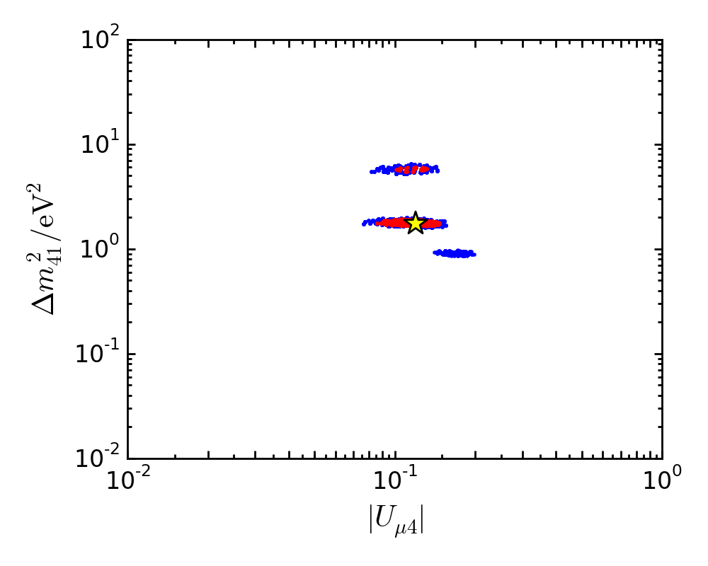
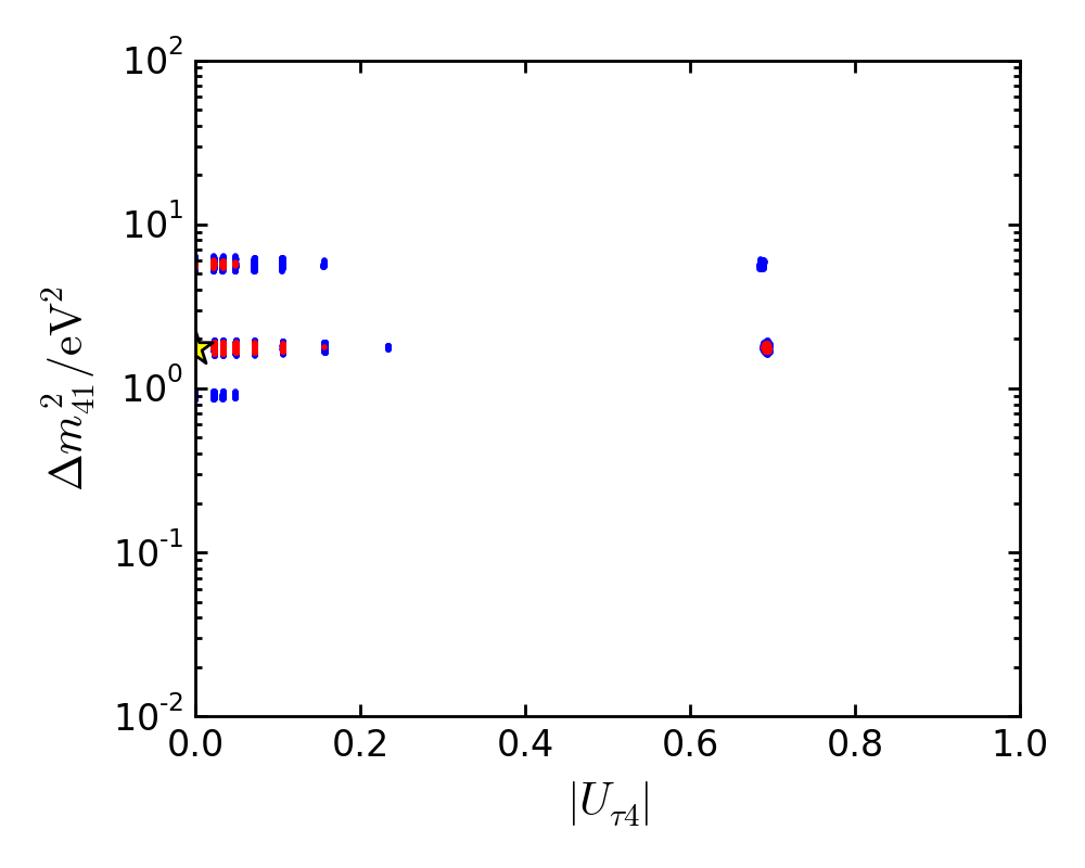
Figs. 2 and 3 show the SBL+IceCube global fit result. The former shows vs , as defined in Eq. 3. The latter presents the result as a function of mixing matrix element. The result is presented on a linear scale because one test point, the preferred solution, is
The IceCube data excludes the solution at eV2 at 90% CL, although that solution persists at 99% CL. This has important implications for future sterile neutrino searches designed to address the 1 eV2 allowed region. For example, given the peak energy of the BNB neutrino beam [25], the position of the ICARUS T600 detector at Fermilab will result in a large potential signal for 1 eV2 sterile neutrino, but less so if the is higher.
As discussed, the SBL experiments constrain and , while the IceCube analysis has strong dependence on and through the matter-induced resonance. Thus, including IceCube provides insight into the less explored parameter. Using , we convert the results to the 90% C.L. ranges in Tab. 2. At eV2, our limit improves the bound of at 90% C.L. from MINOS [66] by a factor of four.
For the first time, this new result on allows us to have a complete picture of the extended lepton mixing matrix:
| (6) |
Above, “…” represents parameters constrained by the overall unitarity of the matrix. The ranges in the matrix correspond to 90% confidence intervals. The entries in the last column correspond to this work and are given for (). The intervals shown in each entry for the standard submatrix were obtained from Ref. [67], and are independent of our fit. As a check of consistency, our values in the fourth column can be compared with the upper bounds from the non-unitarity analysis in Ref. [67], which gave , , and at 90%CL. Our results in Eq. 6 are fully compatible with these upper limits, which are based on standard 3-neutrino oscillation measurements exclusive of any sterile neutrino search data.
V Conclusion
We have presented three new results. First, we have presented a combined fit of SBL and IceCube data resulting in a best fit of with of 50.61 for 4 dof, which is not significantly different from past recent fits [21]. Instead, the significance of the IceCube data is that it substantially lessens the likelihood of the eV2 allowed region that was, until recently, the best fit point [68], and which has formed the basis of the design of many planned sterile neutrino searches. Thus, despite not changing the best fit point, IceCube has significantly altered the sterile neutrino landscape. Second, we have shown that this fit is sensitive to , providing improved constraint on of at 90% C.L. for . Lastly, we have used this, along with constraints from fits to atmospheric and solar data sets, to fill in all components of the 3+1 mixing matrix for the first time.
Acknowledgements
GC, CA and JC are supported by NSF grants 1505858 and 1505855, and MS is supported by NSF grant 1404209. We thank Kevork Abazajian, Christina Ignarra, Benjamin Jones, William Louis, and Jordi Salvado for useful discussion. We thank Maxim Goncharov for computing support.
References
- Olive et al. [2014] K. A. Olive et al. (Particle Data Group), Chin. Phys. C38, 090001 (2014).
- Gonzalez-Garcia et al. [2014] M. Gonzalez-Garcia, M. Maltoni, and T. Schwetz, Journal of High Energy Physics 2014, 52 (2014), URL http://dx.doi.org/10.1007/JHEP11%282014%29052.
- Aguilar-Arevalo et al. [2001] A. Aguilar-Arevalo et al. (LSND Collaboration), Phys. Rev. D 64, 112007 (2001).
- Aguilar-Arevalo et al. [2013] A. A. Aguilar-Arevalo et al. (MiniBooNE), Phys. Rev. Lett. 110, 161801 (2013), eprint 1207.4809.
- Aguilar-Arevalo et al. [2009a] A. A. Aguilar-Arevalo et al. (MiniBooNE), Phys. Rev. Lett. 102, 101802 (2009a), eprint 0812.2243.
- Declais et al. [1995] Y. Declais, J. Favier, A. Metref, H. Pessard, B. Achkar, et al., Nucl. Phys. B 434, 503 (1995).
- Mention et al. [2011] G. Mention, M. Fechner, T. Lasserre, T. A. Mueller, D. Lhuillier, M. Cribier, and A. Letourneau, Phys. Rev. D83, 073006 (2011), eprint 1101.2755.
- Abdurashitov et al. [2009] J. Abdurashitov et al. (SAGE Collaboration), Phys. Rev. C 80, 015807 (2009).
- Kaether et al. [2010] F. Kaether, W. Hampel, G. Heusser, J. Kiko, and T. Kirsten, Phys. Lett. B 685, 47 (2010).
- ALEPH Collaboration, DELPHI Collaboration, L3 Collaboration, OPAL Collaboration, SLD Collaboration, LEP Electroweak Working Group, SLD Electroweak and Heavy Flavour Groups [2006] ALEPH Collaboration, DELPHI Collaboration, L3 Collaboration, OPAL Collaboration, SLD Collaboration, LEP Electroweak Working Group, SLD Electroweak and Heavy Flavour Groups, Phys. Rept. 427, 257 (2006).
- Armbruster et al. [2002] B. Armbruster et al. (KARMEN Collaboration), Phys. Rev. D 65, 112001 (2002).
- Conrad and Shaevitz [2012] J. Conrad and M. Shaevitz, Phys. Rev. D 85, 013017 (2012).
- Adamson et al. [2009a] P. Adamson et al. (MiniBooNE and MINOS Collaborations), Phys. Rev. Lett. 102, 211801 (2009a).
- Aguilar-Arevalo et al. [2009b] A. A. Aguilar-Arevalo et al. (MiniBooNE Collaboration), Phys. Rev. Lett. 103, 061802 (2009b).
- Cheng et al. [2011] G. Cheng et al. (SciBooNE Collaboration), Phys. Rev. D 84, 012009 (2011).
- Astier et al. [2003] P. Astier et al. (NOMAD Collaboration), Phys. Lett. B 570, 19 (2003).
- Stockdale et al. [1985] I. Stockdale, A. Bodek, F. Borcherding, N. Giokaris, K. Lang, et al., Z. Phys. C 27, 53 (1985).
- Dydak et al. [1984] F. Dydak, G. Feldman, C. Guyot, J. Merlo, H. Meyer, et al., Phys. Lett. B 134, 281 (1984).
- D.G. Michael et al. (2006) [MINOS Collaboration] D.G. Michael et al. (MINOS Collaboration), Phys. Rev. Lett. 97, 191801 (2006).
- P. Adamson et al. (2008a) [MINOS Collaboration] P. Adamson et al. (MINOS Collaboration), Phys. Rev. Lett. 101, 131802 (2008a).
- Collin et al. [2016] G. H. Collin, C. A. Argüelles, J. M. Conrad, and M. H. Shaevitz, Nucl. Phys. B908, 354 (2016), eprint 1602.00671.
- Kopp et al. [2013] J. Kopp, P. A. N. Machado, M. Maltoni, and T. Schwetz, Journal of High Energy Physics 2013 (2013), ISSN 1029-8479, arXiv: 1303.3011, URL http://arxiv.org/abs/1303.3011.
- Giunti et al. [2013] C. Giunti, M. Laveder, Y. F. Li, and H. W. Long, Physical Review D 88 (2013), ISSN 1550-7998, 1550-2368, arXiv: 1308.5288, URL http://arxiv.org/abs/1308.5288.
- H. Chen et al. (2007) [MicroBooNE Collaboration] H. Chen et al. (MicroBooNE Collaboration) (2007), eprint “Proposal for a New Experiment Using the Booster and NuMI Neutrino Beamlines: MicroBooNE”, URL http://www-microboone.fnal.gov/public/MicroBooNE_10152007.pdf.
- Antonello et al. [2015] M. Antonello et al. (LAr1-ND, ICARUS-WA104, MicroBooNE) (2015), eprint 1503.01520.
- Adelmann et al. [2014] A. Adelmann, J. Alonso, W. A. Barletta, J. M. Conrad, M. H. Shaevitz, J. Spitz, M. Toups, and L. A. Winslow, Adv. High Energy Phys. 2014, 347097 (2014), eprint 1307.6465.
- Langford [2015] T. J. Langford (PROSPECT), Nucl. Part. Phys. Proc. 265-266, 123 (2015), eprint 1501.00194.
- Bravo-Berguño et al. [2016] D. Bravo-Berguño et al. (SOX), Nucl. Part. Phys. Proc. 273-275, 1760 (2016).
- Aartsen et al. [2016] M. G. Aartsen et al. (IceCube) (2016), eprint 1605.01990.
- Aguilar-Arevalo et al. [2007] A. A. Aguilar-Arevalo et al. (MiniBooNE), Phys. Rev. Lett. 98, 231801 (2007), eprint 0704.1500.
- Aguilar-Arevalo et al. [2010] A. A. Aguilar-Arevalo et al. (MiniBooNE), Phys. Rev. Lett. 105, 181801 (2010), eprint 1007.1150.
- Adamson et al. [2009b] P. Adamson et al. (MiniBooNE, MINOS), Phys. Rev. Lett. 102, 211801 (2009b), eprint 0809.2447.
- Mahn et al. [2012] K. B. M. Mahn et al. (SciBooNE, MiniBooNE), Phys. Rev. D85, 032007 (2012), eprint 1106.5685.
- Cheng et al. [2012] G. Cheng et al. (SciBooNE, MiniBooNE), Phys. Rev. D86, 052009 (2012), eprint 1208.0322.
- P. Adamson et al. (2008b) [MINOS Collaboration] P. Adamson et al. (MINOS Collaboration), Phys. Rev. D 77, 072002 (2008b).
- An et al. [2016] F. P. An et al. (Daya Bay) (2016), eprint 1607.01174.
- Adamson et al. [2016] P. Adamson et al. (MINOS), Submitted to: Phys. Rev. Lett. (2016), eprint 1607.01176.
- Adamson et al. [2011a] P. Adamson et al. (MINOS), Phys. Rev. Lett. 107, 181802 (2011a), eprint 1108.0015.
- Abazajian and Kaplinghat [2016] K. N. Abazajian and M. Kaplinghat, Ann Rev. Nuc. Part. Phys. 66, 401 (2016).
- Abazajian [2003] K. N. Abazajian, Astropart. Phys. 19, 303 (2003), eprint astro-ph/0205238.
- Dasgupta and Kopp [2014] B. Dasgupta and J. Kopp, Phys. Rev. Lett. 112, 031803 (2014), eprint 1310.6337.
- Hannestad et al. [2014] S. Hannestad, R. S. Hansen, and T. Tram, Phys. Rev. Lett. 112, 031802 (2014), eprint 1310.5926.
- Bento and Berezhiani [2001] L. Bento and Z. Berezhiani, Phys. Rev. D64, 115015 (2001), eprint hep-ph/0108064.
- Chu and Cirelli [2006] Y.-Z. Chu and M. Cirelli, Phys. Rev. D74, 085015 (2006), eprint astro-ph/0608206.
- Foot and Volkas [1995] R. Foot and R. R. Volkas, Phys. Rev. Lett. 75, 4350 (1995), eprint hep-ph/9508275.
- Gelmini et al. [2004] G. Gelmini, S. Palomares-Ruiz, and S. Pascoli, Phys. Rev. Lett. 93, 081302 (2004), eprint astro-ph/0403323.
- Ho and Scherrer [2013] C. M. Ho and R. J. Scherrer, Phys. Rev. D87, 065016 (2013), eprint 1212.1689.
- Hamann et al. [2011] J. Hamann, S. Hannestad, G. G. Raffelt, and Y. Y. Y. Wong, JCAP 1109, 034 (2011), eprint 1108.4136.
- Abazajian et al. [2005] K. Abazajian, N. F. Bell, G. M. Fuller, and Y. Y. Y. Wong, Phys. Rev. D72, 063004 (2005), eprint astro-ph/0410175.
- Archidiacono et al. [2016] M. Archidiacono, S. Gariazzo, C. Giunti, S. Hannestad, R. Hansen, M. Laveder, and T. Tram, JCAP 1608, 067 (2016), eprint 1606.07673.
- Nunokawa et al. [2003] H. Nunokawa, O. L. G. Peres, and R. Zukanovich Funchal, Phys. Lett. B562, 279 (2003), eprint hep-ph/0302039.
- Choubey [2007] S. Choubey, JHEP 12, 014 (2007), eprint 0709.1937.
- Razzaque and Smirnov [2012] S. Razzaque and A. Yu. Smirnov, Phys. Rev. D85, 093010 (2012), eprint 1203.5406.
- Esmaili and Smirnov [2013] A. Esmaili and A. Yu. Smirnov, JHEP 12, 014 (2013), eprint 1307.6824.
- Barger et al. [2012] V. Barger, Y. Gao, and D. Marfatia, Phys. Rev. D85, 011302 (2012), eprint 1109.5748.
- Esmaili et al. [2012] A. Esmaili, F. Halzen, and O. L. G. Peres, JCAP 1211, 041 (2012), eprint 1206.6903.
- Esmaili et al. [2013] A. Esmaili, F. Halzen, and O. L. G. Peres, JCAP 1307, 048 (2013), eprint 1303.3294.
- Parke and Ross-Lonergan [2015] S. Parke and M. Ross-Lonergan (2015), eprint 1508.05095.
- Arguelles Delgado et al. [2014] C. A. Arguelles Delgado, J. Salvado, and C. N. Weaver (2014), eprint 1412.3832.
- [60] C. A. Arguelles Delgado, J. Salvado, and C. N. Weaver, -SQuIDS, https://github.com/arguelles/nuSQuIDS.
- Dziewonski and Anderson [1981] A. M. Dziewonski and D. L. Anderson, Physics of the Earth and Planetary Interiors 25, 297 (1981).
- Gonzalez-Garcia et al. [2005] M. C. Gonzalez-Garcia, F. Halzen, and M. Maltoni, Phys. Rev. D71, 093010 (2005), eprint hep-ph/0502223.
- Arguelles et al. [2015] C. A. Arguelles, F. Halzen, L. Wille, M. Kroll, and M. H. Reno, Phys. Rev. D92, 074040 (2015), eprint 1504.06639.
- Cooper-Sarkar et al. [2011] A. Cooper-Sarkar, P. Mertsch, and S. Sarkar, JHEP 08 (2011), eprint 1106.3723, URL http://arxiv.org/abs/1106.3723.
- Lindner et al. [2015] M. Lindner, W. Rodejohann, and X.-J. Xu (2015), eprint 1510.00666.
- Adamson et al. [2011b] P. Adamson et al. (MINOS), Phys. Rev. Lett. 107, 011802 (2011b), eprint 1104.3922.
- Parke and Ross-Lonergan [2016] S. Parke and M. Ross-Lonergan (2016), private communication.
- Conrad et al. [2013] J. M. Conrad, C. M. Ignarra, G. Karagiorgi, M. H. Shaevitz, and J. Spitz, Adv. High Energy Phys. 2013, 163897 (2013), eprint 1207.4765.
- Honda et al. [2004] M. Honda, T. Kajita, K. Kasahara, and S. Midorikawa, Phys. Rev. D 70, 043008 (2004).
- [70] http://icecube.wisc.edu/science/data/IC86-sterile-neutrino.
- Jones [2015] B. J. P. Jones, Ph.D. thesis, MIT (2015), URL http://lss.fnal.gov/archive/thesis/2000/fermilab-thesis-2015-17.pdf.
- Arguelles Delgado [2015] C. A. Arguelles Delgado, Ph.D. thesis, University of Wisconsin - Madison (2015), URL http://search.proquest.com/docview/1720322773.
Appendix: Incorporating the IceCube Data Into the Fits
The fits proceed by first obtaining the prediction for IceCube for a given 3+1 model. To obtain this, we use the Honda-Gaisser [69] prediction for the unoscillated flux. The nuSQuIDS package [60] is used to propagate the neutrino flux across the Earth. The software solves the neutrino evolution “master equation” that accounts for absorption, regeneration and oscillations (Eqs. (29-30) in Ref. [62]). A propagated flux hypothesis is used to produce a weight for each neutrino energy, zenith angle and flavor at the detector. This can then be used to re-weight the IceCube simulated events available in Ref. [70].
The IceCube likelihood is given by [71, 72, 29]:
| (7) |
where are the number of events in the ith bin, is the MC expectation in the same bin, given nuisance parameters () and oscillation parameters ().
We include the nuisance parameters specified in [70, 71, 72, 29]. We maximize the likelihood as a function of flux variants at each parameter point. We note this is an important step in reproducing the IceCube limit.
In Supplementary Figure 1, we show the IceCube 90% CL limit obtained by this analysis. As expected, the result for , shown by the solid line, is in agreement with that presented in Refs. [71, 72, 29] for the “rate+shape” analysis. This limit is modified at high if is nonzero, as discussed in Ref. [65]. We illustrate the effect with the 90% CL limit for IceCube assuming , shown by the dashed line. Also overlaid on this plot is the global fit result, including the IceCube result, expressed as a function of vs .
In order to combine the IceCube result with the other experiments in Table 1 of Ref. [21], the IceCube likelihood must be converted to a that can be combined with that of the global fit. In order to do this, it is convenient to use:
| (8) |
where is the saturated Poisson. In the fitting code, we implement Eq. 7, and in Tab. 1 we use Eq. 8, following the same procedure as for LSND and Karmen in Ref. [21]. (The definitions in Eq. 7 and Eq. 8 give the same used for fitting and parameter estimation.)
The high computational cost of propagating neutrino fluxes through the Earth with nuSQuIDS prevents the analysis from being directly included into the global fitting software. Instead, the global fits were used to find a reduced set of parameters (called “parameter-set points” below) that could be evaluated directly. The 60,000 parameter-set points for the SBL global fits from Ref. [21], i.e. without IceCube data included, with the lowest were used. From these every 40th point was selected. This gave a fine sampling of the global fit near the minima. Of the remaining 140,000 parameter-set points that are far from the minima, every 60th was selected. Combining the fine sample and the coarse sample yields 4,000 points. These 4,000 selected parameter-set points only explored changes in the values for and . In order to incorporate the IceCube data and effects of , ten values of the angle were chosen for each parameter point, resulting in a total of 40,000 parameter-set points. These points were fed into the IceCube analysis likelihood and the resulting value, defined by Eq. 8, was combined with the respective frequentist global fit .
This assumes that the effect of IceCube on the global fit is a small perturbation. This is reasonable given that the IceCube-only is small compared to the SBL only global fit , as shown in Table 1.
