Constraining stellar binary black hole formation scenarios with eLISA eccentricity measurements
Abstract
A space-based interferometer such as eLISA could observe few to few thousands progenitors of black hole binaries (BHBs) similar to those recently detected by Advanced LIGO. Gravitational radiation circularizes the orbit during inspiral, but some BHBs retain a measurable eccentricity at the low frequencies where eLISA is most sensitive. The eccentricity of a BHB carries precious information about its formation channel: BHBs formed in the field, in globular clusters, or close to a massive black hole (MBH) have distinct eccentricity distributions in the eLISA band. We generate mock eLISA observations, folding in measurement errors, and using Bayesian model selection we study whether eLISA measurements can identify the BHB formation channel. We find that a handful of observations would suffice to tell whether BHBs were formed in the gravitational field of a MBH. Conversely, several tens of observations are needed to tell apart field formation from globular cluster formation. A five-year eLISA mission with the longest possible armlength is desirable to shed light on BHB formation scenarios.
keywords:
black hole physics - gravitational waves1 Introduction
The first direct observation of merging black hole binaries (BHBs) during the first observation run (O1) of Advanced LIGO marked a milestone in the history of astronomy and fundamental physics. The observation of two events (GW150914 and GW151226), plus a third candidate LVT151012 (Abbott et al., 2016d, a, b), provides a formidable laboratory to test general relativity in the strong-gravity regime (Abbott et al., 2016e). In addition, gravitational-wave observations of BHBs can further our understanding of their astrophysical formation channels (Abbott et al., 2016f). Different formation scenarios result in distinct BHB binary properties, that may be disentangled by analysing the statistical parameters of a sufficiently large number of detections. The currently favoured scenarios involve stellar evolution of field binaries (Benacquista & Downing, 2013) and the dynamical capture of BHs in globular clusters (Postnov & Yungelson, 2014). Recent work showed that both field formation (Mapelli et al., 2009; Belczynski et al., 2010; Dominik et al., 2012, 2013; Spera et al., 2015; Dominik et al., 2015; Belczynski et al., 2016a; Belczynski et al., 2016b) and cluster formation (Rodriguez et al., 2015; Rodriguez et al., 2016a; Chatterjee et al., 2016; Rodriguez et al., 2016b) are compatible with the recent Advanced LIGO observations (Abbott et al., 2016f). More exotic proposals include formation via hierarchical triples in the background of a MBH (Antonini et al., 2016), a Population III origin for the binary members (Kinugawa et al., 2014; Hartwig et al., 2016), chemically homogeneous evolution in short-period binaries (Mandel & de Mink, 2016; de Mink & Mandel, 2016), massive overcontact binary evolution (Marchant et al., 2016), and even primordial BHs (Bird et al., 2016).
In the field formation scenario BHBs have very small eccentricities in the Advanced LIGO band, and the BH spins should be preferentially aligned with the orbital angular momentum as a consequence of mass transfer episodes preceding the stellar collapse. In the globular cluster scenario BHBs are formed via BH capture on eccentric orbits, and the spins of the two BHs are likely to be randomly oriented. Earth-based gravitational-wave observations could potentially differentiate between field and cluster formation by looking at spin dynamics, redshift distribution and possibly kicks. However the details of mass transfer and tidal alignment in BH binaries, as well as the degree of asymmetry in stellar collapse – and the resulting kicks imparted to the BHs – are quite uncertain, and they will affect BH spin alignment and gravitational waveforms in complex ways (Belczynski et al., 2008; Gerosa et al., 2013, 2015; Belczynski et al., 2016a). In this respect, eccentricity may be a more robust tracer of the formation channel. Radiation reaction is well known to circularize the orbit. While field and cluster formation scenarios predict very distinct eccentricity distributions at BHB formation, both scenarios result in nearly circular binaries in the Advanced LIGO band. The first observed signals did not set strong bounds on the eccentricity of the binary (Abbott et al., 2016c, b), and it is quite unlikely that eccentricity measurements with ground-based detectors will ever differentiate between the field and cluster scenarios. However, Sesana (2016) showed that, depending on the intrinsic rates (which are only loosely constrained by current detections) and on the detector baseline, the evolved Laser Interferometer Space Antenna (eLISA) will observe few to few thousands BHBs (see also Kyutoku & Seto, 2016). Because of the much lower frequency band, eLISA will detect these systems before circularization, and in many cases it will be able to measure their eccentricity (Nishizawa et al., 2016).
In this Letter we use Bayesian model selection to demonstrate how eLISA eccentricity measurement can conclusively distinguish between different BHB formation channels. In Section II we consider three models for BHB formation, and discuss the eccentricity distributions predicted by these models in the eLISA band111For a detailed astrophysical comparison of BHBs formed in galactic fields and globular clusters observable by eLISA, see Breivik et al. (2016).. In Section III we simulate and analyse eLISA observations using various models and detector baselines. In Section IV we present our main results, and in Section V we discuss their implications. We assume a concordance CDM cosmology with , and (Planck Collaboration et al., 2015).
2 Astrophysical models and eccentricity distributions
We consider a BHB population merging at a rate , characterized by a chirp mass probability distribution – where , and a subscript denotes quantities in the rest frame of the source – and by an eccentricity probability distribution at some reference frequency close to coalescence (we set Hz). If depends only on the BHB formation route, but not on chirp mass and redshift, the merger rate density per unit mass and eccentricity is given by
| (1) |
Equation (1) can be then converted into a number of sources emitting per unit mass, redshift and frequency at any time via
| (2) |
where is the standard volume shell per unit redshift, and
| (3) |
Here
| (4) |
and is computed by finding the root of
| (5) |
We can construct a population of systems potentially observable by eLISA by Monte Carlo sampling from the distribution in equation (2) using appropriate distribution functions for and . For the mass distribution we employ the “flat” mass function of Abbott et al. (2016f), i.e., we assume that the two BH masses are independently drawn from a log-flat distribution in the range , restricting the total BHB mass to the be less than . For the eccentricity distribution we consider, as a proof of concept, three popular BHB formation scenarios:
-
1.
Model field: this is the default BHB field formation scenario of Kowalska et al. (2011), taken to be representative of BHBs resulting from stellar evolution.
-
2.
Model cluster: globular clusters efficiently form BHBs via dynamical capture. Most of these BHBs are ejected in the field and evolve in isolation until they eventually merge. Because of their dynamical nature, BHBs typically form with a thermal eccentricity distribution. A comprehensive study of this scenario has been performed by Rodriguez et al. (2016c).
-
3.
Model MBH. BHs and BHBs are expected to cluster in galactic nuclei because of strong mass segregation. In this case, binaries within the sphere of influence of the central MBH undergo Kozai-Lidov resonances, forming triplets in which the external perturber is the MBH itself. This scenario has been investigated in Antonini & Perets (2012), and it results in high BHB eccentricities.
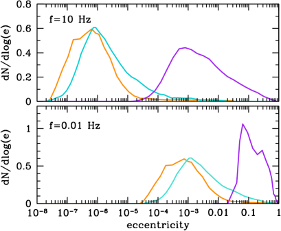
The eccentricity distributions at Hz, as predicted by these models, are shown in the top panel of Figure 1. In the bottom panel we propagate these distributions “back in time” to obtain at frequency Hz, where most eLISA detections are expected to occur. In this calculation we must take into account the fact that highly eccentric binaries evolve more quickly – by a factor – than circular ones, so that only a few highly eccentric binaries will be observable in the eLISA band for a given coalescence rate.
3 Simulations and analysis tools
We consider two eLISA baselines, N2A2 and N2A5 in the notation of Klein et al. (2016). We adopt the noise level (N2) recently demonstrated by LISA Pathfinder (LPF, Armano et al., 2016) and, following the recommendations of the GOAT committee222http://www.cosmos.esa.int/web/goat, we choose armlengths of two (A2) and five (A5) million kilometers. We also explore two nominal mission lifetimes (2 and 5 years) for a total of four mission baselines: N2A2-2y, N2A2-5y, N2A5-2y, N2A5-5y.
For our simulated experiments we need (a) the theoretical eccentricity distribution predicted by the three BHB formation models, and (b) catalogues of “synthetic” eLISA observations to be tested against the models. The theoretical distributions are generated as follows: (i) Following the formalism described in Section 2, for each model we generate a large Monte Carlo catalogue of BHBs emitting in the eLISA frequency window; (ii) For each eLISA baseline, we select a sample of detectable BHBs with and construct their eccentricity distribution; (iii) We fit a smooth polynomial function to each distribution. This procedure yields 12 theoretical eccentricity distributions to be tested against observations for each setup (i.e., for each combination of BHB formation model and eLISA baseline).
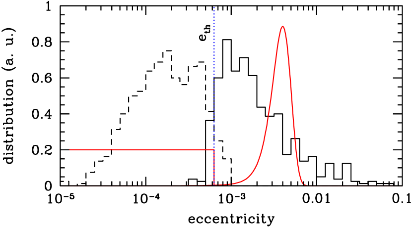
The next step is the generation of synthetic BHB observations. We select detectable events with (because of computational limitations) and with eccentricity smaller than when eLISA observations begin (because of limitations in our waveform model, that becomes unreliable for high eccentricities). For each of these events we compute the error in the measurement of the binary eccentricity using the Fisher information matrix, as described in Nishizawa et al. (2016). For any given number of observed BHBs, we draw 100 random catalogues of systems from the simulated detections.
As shown by Nishizawa et al. (2016), eLISA will enable precise measurements of down to , with mild dependence on armlength or observation time. Roughly speaking, as shown in Figure 2, this means that can be measured above some threshold . To fold in error measurements into each catalogue, we split the events in two classes: 1) if the eccentricity is measurable, and we assign to the eccentricity a probability distribution , where the measured value is drawn from a Gaussian distribution centred in with variance ; 2) if we simply assume that we have an upper limit on , that we take to be for simplicity. Therefore is just a step function: for , and for . Examples of this procedure are shown in Figure 2.
For each setup and each this procedure yields 100 catalogues of observed events, each characterized by the appropriate . The 100 catalogues are not independent when , since most of them will share some events. However, even for the “shared” events is obtained from a different random draw each time, and therefore is different in different catalogues. We checked that the results presented in the next section are unaffected when we consider a smaller number of truly independent catalogues (e.g., 10 catalogues with ). We are therefore confident that our results are robust with respect to statistical fluctuations.
3.1 Statistical analysis
For a given eLISA baseline, our main goal is to consider catalogues of observed events from model (chosen among field, cluster, MBH) and assess to what confidence (if any) we can say whether the underlying astrophysical model was in fact , or an alternative model . This is a classic Bayesian model selection problem. To compare two models and we must compute the odds ratio
| (6) |
where is the evidence of model and is the prior belief that model is right. In absence of prior information, we conservatively assume . Moreover, for non-parametric models (i.e. models without free parameters, as those considered here), the evidence is simply the likelihood of the data given the model. The odds ratio then reduces to the likelihood ratio
| (7) |
In our case, for each set of measurements we have probability distributions of measured eccentricity to be compared to the theoretical eccentricity distribution predicted by a given model, . The likelihood of the data given the model is therefore given by:
| (8) |
In this framework, we can also assign to model a probability and to model the complementary probability . From equation (7), . It is therefore natural to associate the odds ratio with the “confidence” in a given model. For example, if then , and we can say that model is favoured at (95% confidence). Definitive identification can be associated to .
For each of the 100 catalogues of detections, generated for each setup, we compute the likelihood of the observed data against each model: field, cluster, MBH. If the observations can discriminate between different models, the odds ratio will favour the actual model from which the data were drawn. For each comparison we then compute the probabilities and defined above, which describe our degree of confidence that the data were actually drawn from either of the models considered in the comparison.
4 Results
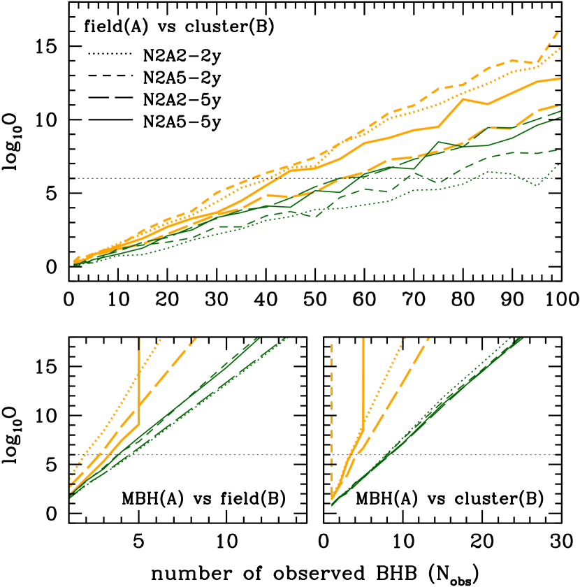
In Figure 3 we compare the median log as a function of for each pair of models. The median is computed over 100 Monte Carlo catalogues for each value of . The two lower panels show that, regardless of the detector baseline, model MBH can be confidently separated – with , i.e. at approximately – from any other model after a handful of observations. This is because the eccentricity distribution for model MBH is biased towards high values (see Figure 1), at variance with other models. Note also that it is easier to reject model MBH when it is false (orange curves) than to confirm it when it is true (green curves). This is because models field and cluster allow for low eccentricities, that are not supported by model MBH (Figure 1). As soon as a BHB has a measured eccentricity , model MBH is automatically rejected. The converse is not true: the eccentricity range of model MBH is also supported by the other models. Therefore, when BHB formation is indeed described by model MBH there is always a chance that highly eccentric BHBs were drawn from other models, and a few more detections are required to reject them. Models field and cluster, on the other hand, predict similar eccentricity distributions,. Depending on which one was the true model and on the eLISA baseline, a number of detections between 30 and 95 is needed to achieve the threshold.
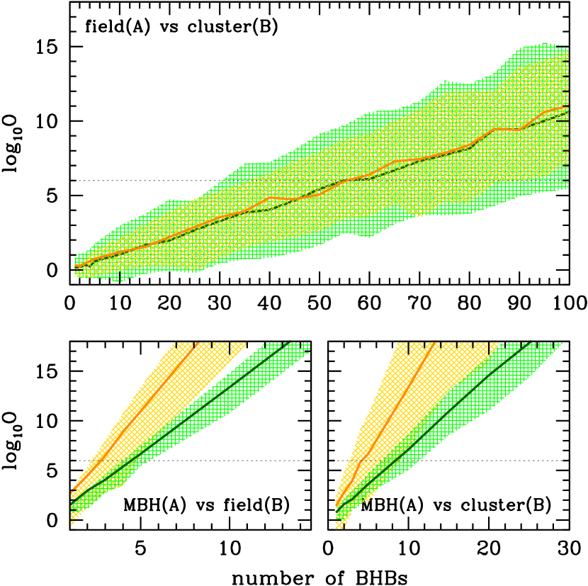
Since all detector baselines yield similar results, we take a closer look at the N2A2-5y case, a plausible “minimum” eLISA baseline target. In Figure 4 we show odds ratios for this specific configuration, including the 90% confidence interval computed from the 100 catalogues constructed for each . The log threshold is always achieved with less than 10 observed BHBs when the MBH model is involved in the comparison, whereas up to 100 BHBs may be needed to discriminate between the field and cluster models, depending on the specific ensemble of observed BHBs.
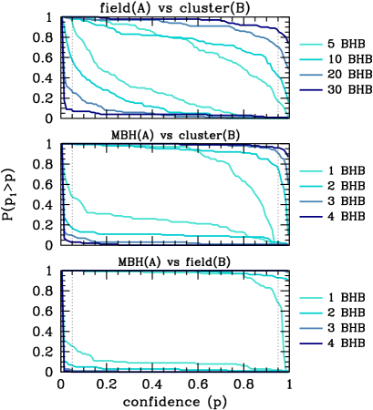
When comparing two models and for a given eLISA baseline, we can use the 100 catalogues at fixed to construct cumulative distributions functions (CDFs) of and (Sesana et al., 2011). Suppose that, in a comparison between models and , is the right model, and we draw 100 realizations of observations from model A. we can compute the associated CDF of and plot it against the confidence (). The result for different values of is shown in the upper curves of each panel of Figure 5. We can also draw 100 realizations of observations from and compute the CDF of when is not true. The result are the lower curves in each panel of Figure 5.
Set, for example, (approx ). The value of the upper curve at is the fraction of realizations for which we have more than confidence that model A is correct when it is, in fact, true. The value of the lower curve at is the fraction of realization for which we cannot rule out model at confidence when it is the wrong model (i.e., observations are generated by model ). Figure 5 presents a similar analysis for all pairs of models assuming the N2A2-5y baseline. About 30 BHB observations are required for a –confidence identification of model field against model cluster in about 90% of the realizations. The same level of confidence requires only 4 and 2 BHBs when model MBH is compared to models cluster and field, respectively.
5 Discussion and outlook
| 3 | 5 | ||||
|---|---|---|---|---|---|
| eLISA base | |||||
| N2A2-2y | 11-78 | 35 | 100 | 95 | 100 |
| N2A5-2y | 85-595 | 34 | 95 | 80 | 100 |
| N2A2-5y | 45-310 | 25 | 60 | 61 | 100 |
| N2A5-5y | 330-2350 | 25 | 62 | 60 | 100 |
For the log-flat distribution assumed here, the Advanced LIGO observations imply a 90% credible interval for the merger rate of yr-1Gpc-3 (Abbott et al., 2016b). The resulting range in is reported in Table 1 for the different baselines, and it should be compared to the number of events needed to discriminate among different models at a desired confidence threshold. Model MBH can be identified by all the configurations with just a few BHB observations, therefore it is not reported in the table. Discriminating between the cluster and field scenarios requires tens of events, and only the baseline N2A5-5y can guarantee a 5 confidence with 90% probability. Baselines N2A2-5y and N2A5-2y can distinguish among these models at the 3 level, but this may not be possible should the event rate lean toward the lower limit of the allowed range. The N2A2-2y baseline performs relatively poorly, and it may not deliver enough detections to pin down the formation mechanism.
These results highlight the importance of aiming for a five-year mission with the longest possible armlength. However, we should bear in mind some limitations of our proof-of-principle analysis. First of all, we selected three representative models from the literature: this does not fully capture all of the relevant physics affecting the eccentricity distribution of BHBs. For example, several variations of the “fiducial” model of Kowalska et al. (2011) result in slightly different eccentricity distributions. Our analysis can be applied systematically to any such variation, assessing to what extent the underlying physics can be constrained. Secondly, we assumed the eccentricity distribution to be independent of masses and redshifts. In practice, different formation channels will result in different mass-eccentricity (and possibly redshift-eccentricity, or spin-eccentricity) correlations, that can be exploited in a multi-dimensional analysis to enhance the discriminating power of the observations. Finally, it is very likely that several different formation channels operate at the same time in the Universe. In the context of massive BHB observations, Sesana et al. (2011) studied whether eLISA could identify a superposition of distinct formation channels from the statistical properties of the observed population. A similar analysis in the present context is an interesting topic for future work.
Acknowledgements
A.S. thanks T. Dent and A. Vecchio for useful discussions. E.B., A.K. and A.N. are supported by NSF CAREER Grant No. PHY-1055103. E.B. and A.K. are supported by FCT contract IF/00797/2014/CP1214/CT0012 under the IF2014 Programme. This work was supported by the H2020-MSCA-RISE- 2015 Grant No. StronGrHEP-690904. A.S. is supported by a University Research Fellowship of the Royal Society.
References
- Abbott et al. (2016b) Abbott B. P., et al., 2016b, preprint, (arXiv:1606.04856)
- Abbott et al. (2016a) Abbott B. P., et al., 2016a, preprint, (arXiv:1606.04855)
- Abbott et al. (2016c) Abbott B. P., Abbott R., Abbott T. D., Abernathy M. R., Acernese F., Ackley K., et al. 2016c, preprint, (arXiv:1602.03840)
- Abbott et al. (2016d) Abbott B. P., et al., 2016d, Physical Review Letters, 116, 061102
- Abbott et al. (2016e) Abbott B. P., et al., 2016e, Physical Review Letters, 116, 221101
- Abbott et al. (2016f) Abbott B. P., et al., 2016f, ApJ, 818, L22
- Antonini & Perets (2012) Antonini F., Perets H. B., 2012, Astrophys. J., 757, 27
- Antonini et al. (2016) Antonini F., Chatterjee S., Rodriguez C. L., Morscher M., Pattabiraman B., Kalogera V., Rasio F. A., 2016, Astrophys. J., 816, 65
- Armano et al. (2016) Armano M., et al., 2016, Physical Review Letters, 116, 231101
- Belczynski et al. (2008) Belczynski K., Taam R. E., Rantsiou E., van der Sluys M., 2008, ApJ, 682, 474
- Belczynski et al. (2010) Belczynski K., Dominik M., Bulik T., O’Shaughnessy R., Fryer C., Holz D. E., 2010, ApJ, 715, L138
- Belczynski et al. (2016a) Belczynski K., Holz D. E., Bulik T., O’Shaughnessy R., 2016a, preprint, (arXiv:1602.04531)
- Belczynski et al. (2016b) Belczynski K., Repetto S., Holz D. E., O’Shaughnessy R., Bulik T., Berti E., Fryer C., Dominik M., 2016b, ApJ, 819, 108
- Benacquista & Downing (2013) Benacquista M. J., Downing J. M. B., 2013, Living Reviews in Relativity, 16
- Bird et al. (2016) Bird S., Cholis I., Muñoz J. B., Ali-Haïmoud Y., Kamionkowski M., Kovetz E. D., Raccanelli A., Riess A. G., 2016, Physical Review Letters, 116, 201301
- Breivik et al. (2016) Breivik K., Rodriguez C. L., Larson S. L., Kalogera V., Rasio F. A., 2016, preprint
- Chatterjee et al. (2016) Chatterjee S., Rodriguez C. L., Rasio F. A., 2016, preprint, (arXiv:1603.00884)
- Dominik et al. (2012) Dominik M., Belczynski K., Fryer C., Holz D. E., Berti E., Bulik T., Mandel I., O’Shaughnessy R., 2012, ApJ, 759, 52
- Dominik et al. (2013) Dominik M., Belczynski K., Fryer C., Holz D. E., Berti E., Bulik T., Mandel I., O’Shaughnessy R., 2013, ApJ, 779, 72
- Dominik et al. (2015) Dominik M., et al., 2015, ApJ, 806, 263
- Gerosa et al. (2013) Gerosa D., Kesden M., Berti E., O’Shaughnessy R., Sperhake U., 2013, Phys. Rev., D87, 104028
- Gerosa et al. (2015) Gerosa D., Kesden M., Sperhake U., Berti E., O’Shaughnessy R., 2015, Phys. Rev. D, 92, 064016
- Hartwig et al. (2016) Hartwig T., Volonteri M., Bromm V., Klessen R. S., Barausse E., Magg M., Stacy A., 2016, MNRAS,
- Kinugawa et al. (2014) Kinugawa T., Inayoshi K., Hotokezaka K., Nakauchi D., Nakamura T., 2014, MNRAS, 442, 2963
- Klein et al. (2016) Klein A., et al., 2016, Phys. Rev. D, 93, 024003
- Kowalska et al. (2011) Kowalska I., Bulik T., Belczynski K., Dominik M., Gondek-Rosinska D., 2011, Astron. Astrophys., 527, A70
- Kyutoku & Seto (2016) Kyutoku K., Seto N., 2016, preprint, (arXiv:1606.02298)
- Mandel & de Mink (2016) Mandel I., de Mink S. E., 2016, MNRAS, 458, 2634
- Mapelli et al. (2009) Mapelli M., Colpi M., Zampieri L., 2009, MNRAS, 395, L71
- Marchant et al. (2016) Marchant P., Langer N., Podsiadlowski P., Tauris T. M., Moriya T. J., 2016, A&A, 588, A50
- Nishizawa et al. (2016) Nishizawa A., Berti E., Klein A., Sesana A., 2016, preprint, (arXiv:1605.01341)
- Planck Collaboration et al. (2015) Planck Collaboration et al., 2015, preprint, (arXiv:1502.01589)
- Postnov & Yungelson (2014) Postnov K. A., Yungelson L. R., 2014, Living Reviews in Relativity, 17
- Rodriguez et al. (2015) Rodriguez C. L., Morscher M., Pattabiraman B., Chatterjee S., Haster C.-J., Rasio F. A., 2015, Physical Review Letters, 115, 051101
- Rodriguez et al. (2016a) Rodriguez C. L., Chatterjee S., Rasio F. A., 2016a, Phys. Rev. D, 93, 084029
- Rodriguez et al. (2016b) Rodriguez C. L., Haster C.-J., Chatterjee S., Kalogera V., Rasio F. A., 2016b, ApJ, 824, L8
- Rodriguez et al. (2016c) Rodriguez C. L., Chatterjee S., Rasio F. A., 2016c, Phys. Rev., D93, 084029
- Sesana (2016) Sesana A., 2016, Physical Review Letters, 116, 231102
- Sesana et al. (2011) Sesana A., Gair J., Berti E., Volonteri M., 2011, Phys. Rev. D, 83, 044036
- Spera et al. (2015) Spera M., Mapelli M., Bressan A., 2015, MNRAS, 451, 4086
- de Mink & Mandel (2016) de Mink S. E., Mandel I., 2016, MNRAS, 460, 3545