Lattice models for granular-like velocity fields: Finite-size effects

Abstract

Long-range spatial correlations in the velocity and energy fields of a granular fluid are discussed in the framework of a 1d lattice model. The dynamics of the velocity field occurs through nearest-neighbour inelastic collisions that conserve momentum but dissipate energy. A set of equations for the fluctuating hydrodynamics of the velocity and energy mesoscopic fields give a first approximation for (i) the velocity structure factor and (ii) the finite-size correction to the Haff law, both in the homogeneous cooling regime. At a more refined level, we have derived the equations for the two-site velocity correlations and the total energy fluctuations. First, we seek a perturbative solution thereof, in powers of the inverse of system size. On the one hand, when scaled with the granular temperature, the velocity correlations tend to a stationary value in the long time limit. On the other hand, the scaled standard deviation of the total energy diverges, that is, the system shows multiscaling. Second, we find an exact solution for the velocity correlations in terms of the spectrum of eigenvalues of a certain matrix. The results of numerical simulations of the microscopic model confirm our theoretical results, including the above described multiscaling phenomenon.

1 Introduction

Granular materials are systems that comprise a “large” number of macroscopic particles (grains), the collisions between which are inelastic [1]. When the grains inside a container are rapidly shaken, the granular fluid regime appears. Moreover, if the particles move freely between their binary instantaneous collisions, we have a “granular gas”  [2]. This is usually so when the peak acceleration is many times the gravity and the packing fraction is below $\sim\!1\%$. Interestingly, kinetic theory can be extended to the granular case by writing an inelastic version of the Boltzmann equation [3], which takes into account that energy is no longer conserved in collisions.

The number of particles in a granular system is much smaller than Avogadro’s number, and then fluctuations are expected to be more important than those in molecular systems. A promising approach is to study intermediate coarse-graining schemes, such as mesoscospic fluctuating hydrodynamics, to account for the fluctuations of “slow variables” in the system, e.g. those associated to conserved or quasi-conserved quantities such as momentum or energy. Regrettably, there is not a generalisation of the theory of mesoscopic fluctuations valid at equilibrium [4, 5, 6] to the non-equilibrium domain. Nevertheless, some progress have been recently made to derive a consistent fluctuating hydrodynamic picture from the inelastic Boltzmann equation  [7]. Here we choose a different perspective, looking for a simplified model that contains the essential ingredients of granular fluids but reduces the complexity of the task and promises a transparent interpretation of the results. In particular we aim to elucidate the “perturbative” nature of the continuum limit and calculate the corrections to it [8]. Such corrections give interesting information about the structure - in space and time - of the correlated granular fluctuations and reveal new phenomena peculiar of inelastic collisions.

Lattice models are a useful tool in non-equilibrium statistical mechanics. Their simplicity makes it possible to identify the main elements to describe the experimentally relevant behaviour in many different physical situations. More specifically, lattice models have been of paramount importance for understanding rigorously the conditions needed to have a hydrodynamic description, both at the average  [9, 10] and fluctuating [11] levels. Recently, fluctuating hydrodynamics has been employed to derive the large deviation function in the context of energy-conserving models [12, 13, 14, 15] and even in energy-dissipating models [16, 17, 18]. Both in the conservative and non-conservative case, momentum conservation has not been taken into account. This shortcoming may be relevant, since it is known that momentum conservation is linked to the appearance of long-ranged correlations in out-of-equilibrium systems [19, 20].

Very recently, a lattice model for the velocity field with momentum conservation has been put forward [21]. In a previous paper [22], we derived both the average and fluctuating hydrodynamic pictures, and looked into some relevant physical situations, such as the Homogeneous Cooling or Uniform Shear Flow states. In the present paper we focus on the spatial long-range velocity correlations in the Homogeneous Cooling State, which can be partly explained by fluctuating hydrodynamics but require a more refined treatment to be fully investigated. In our study of velocity and energy spatial correlations two original phenomena emerge: a correction to the Haff’s law due to spatial correlations and a multiscaling phenomenon where the total energy fluctuations do not scale with the temperature.

We briefly summarise the organisation of the paper. In section 2, we introduce the microscopic lattice model, its Master Equation and the fluctuating hydrodynamic equations which have been first presented in [21] and discussed in detail in [22]. Section 3 is devoted to the Homogeneous Cooling State (HCS). Therein, we derive the shape of velocity and energy spatial correlations from fluctuating hydrodynamics, and also compute the first order finite size correction to the Haff law. The microscopic equations for the velocity correlations are obtained in section 4. By going to the continuum limit in them, the energy decay in the HCS is computed in a more precise form that is valid for longer times. In section 5, we discuss an exact scheme for the resolution of the microscopic correlation equations, before taking the continuum limit. The presence of multiscaling for the energy fluctuations is presented in section 6, through both numerical results and an approximate theory based on clustering the three-particle correlations. Conclusions and perspectives are presented in section 7. The appendices deal with some technical details that are omitted in the main text.

2 Revision of the model and previous results

In this section, we briefly revise the main aspects of the model introduced in [21], focusing on its continuum, hydrodynamic-like, limit. A more detailed description of the model can be found in [22].

2.1 Dynamics

Let us consider a 1d lattice with $N$ sites. First, we define the dynamics in discrete time: after the $p$-th step of the dynamics, the particle at the $l$-th site has a velocity $v_{l,p}\in$ $\mathcal{R}$. The configuration for the system at time $p$ is denoted as $\bm{v}_{p}\equiv\{v_{1,p},...,v_{N,p}\}$. One individual trajectory of the (Markovian) stochastic process is built in the following way: the configuration of the system changes from time $p$ to time $p+1$ because a pair of nearest neighbours $\left(l,l+1\right)$ is chosen at random and collides inelastically, that is $\bm{v}_{p+1}=\hat{b}_{l}\bm{v}_{p}$ where the operator $\hat{b}_{l}$ transforms the pre-collisional velocities $(v_{l,p},v_{l+1,p})$ into the post-collisional ones $(v_{l,p+1},v_{l+1,p+1})$ and leaves all other sites unaltered. The post-collisional velocities are given by

$$v_{l,p+1} = v_{l,p}-(1+\alpha)\Delta_{l,p}/2$$ (1a)

$$v_{l+1,p+1} = v_{l+1,p}+(1+\alpha)\Delta_{l,p}/2,$$ (1b)

with $\Delta_{l,p}=v_{l,p}-v_{l+1,p}$ and $0<\alpha\leq 1$. In the following we use a notation such that the evolution operator $\hat{b}_{l}$ acts naturally on observables, e.g. $\hat{b}_{l}v_{l,p}=v_{l,p+1}$. Momentum is always conserved, $(\hat{b}_{l}-1)(v_{l,p}+v_{l+1,p})=0$, whereas energy, if $\alpha\neq 1$, is not: $(\hat{b}_{l}-1)(v^{2}_{l,p}+v^{2}_{l+1,p})=(\alpha^{2}-1)\Delta_{l,p}^{2}/2<0$. The collision rule (1), which corresponds to the simplest one used in granular fluids [23], is valid for bulk sites and must be complemented with suitable boundary conditions.

The evolution equation for the velocities can be cast in the form

$$v_{l,p+1}-v_{l,p}=-j_{l,p}+j_{l-1,p},\quad j_{l,p}=\frac{1+\alpha}{2}\Delta_{l,p}\delta_{y_{p},l}.$$ (2)

This is nothing but a discrete continuity equation, in which $j_{l,p}$ is the momentum current from site $l$ to site $l+1$ at time $p$. In (2), $\delta_{y_{p},l}$ is Kronecker’s delta and $y_{p}$ is a homogeneously distributed random integer in $[1,L]$, where $L$ is the number of possible colliding pairs. For periodic boundary conditions, $L=N$, whereas for thermostatted boundaries $L=N+1$ [22].

We have only kinetic energy, which is ${\cal K}_{p}=\sum_{l=1}^{N}e_{l,p}$ at time $p$, where $e_{l,p}=v_{l,p}^{2}$. By squaring (2), the evolution equation for the energy at site $l$ is obtained

$$e_{l,p+1}-e_{l,p}=-J_{l,p}+J_{l-1,p}+d_{l,p}.$$ (3)

Apart from the “flux” term $-J_{l,p}+J_{l-1,p}$, we have a sink term $d_{l,p}$ that stems from the inelasticity of collisions. The energy current $J_{l,p}$ from site $l$ to site $l+1$ and energy dissipation $d_{l,p}$ at site $l$ are

$$J_{l,p}=(v_{l,p}+v_{l+1,p})j_{l,p},\quad d_{l,p}=\frac{\alpha^{2}-1}{4}\left[\delta_{y_{p},l}\Delta_{l,p}^{2}+\delta_{y_{p},l-1}\Delta_{l-1,p}^{2}\right]<0,$$ (4)

respectively.

The above stochastic dynamics generates the trajectories that correspond to the Markov process described by the master equation in continuous time [22]

$$\partial_{\tau}P_{N}(\bm{v},\tau|\bm{v}_{0},\tau_{0})=\omega\sum_{l=1}^{L}\left[\frac{P_{N}(\hat{b}_{l}^{-1}\bm{v},\tau|\bm{v}_{0},\tau_{0})}{\alpha}-P_{N}(\bm{v},\tau|\bm{v}_{0},\tau_{0})\right],$$ (5)

for the conditional probability density $P_{N}(\bm{v},\tau|\bm{v}_{0},\tau_{0})$ of finding the system in state $\bm{v}$ at time $\tau$ provided it was in state $\bm{v}_{0}$ at time $\tau_{0}$. Above, $\omega$ is a constant frequency that determines the time scale and the operator $\hat{b}_{l}^{-1}$ is the inverse of $\hat{b}_{l}$. Thus, $\hat{b}_{l}^{-1}$ changes the post-collisional velocities into the pre-collisional ones when the colliding pair is $(l,l+1)$. Moreover, the increment $\delta\tau_{p}$ of the continuous time $\tau$ at the $p$-th step of the dynamics over each trajectory is given by $\delta\tau_{p}=-(L\omega)^{-1}\ln x$, in which $x$ is a stochastic variable homogeneously distributed in the interval $(0,1)$.

2.2 Hydrodynamic equations

In the large system size limit as $L\to\infty$, a continuum limit may be introduced by considering that the average velocity $u_{l,p}=\langle v_{l,p}\rangle$ and energy $E_{l,p}=\langle v_{l,p}^{2}\rangle$ are smooth functions of space and time. Of course, the local temperature $T_{l,p}=E_{l,p}-u_{l,p}^{2}$ is also smooth. Specifically, we introduce hydrodynamic continuous space and time variables $x=l/L$ and $t=\omega\tau/L^{2}$, respectively.

In this continuum limit, the balance equations for the average velocity $u(x,t)$ and energy $E(x,t)=u^{2}(x,t)+T(x,t)$ read

$$\partial_{t}u(x,t) =-\partial_{x}j_{\text{av}}(x,t),$$ (6a)

$$\partial_{t}E(x,t) =-\partial_{x}J_{\text{av}}(x,t)+d_{\text{av}}(x,t).$$ (6b)

Therein, the average momentum and energy currents, $j_{\text{av}}(x,t)$ and $J_{\text{av}}(x,t)$, respectively, are given by

$$j_{\text{av}}(x,t)=-\partial_{x}u(x,t),\quad J_{\text{av}}(x,t)=-\partial_{x}E(x,t),$$ (7)

and the dissipation field $d_{\text{av}}(x,t)$ is

$$d_{\text{av}}(x,t)=-\nu T,\quad\nu=(1-\alpha^{2})L^{2}.$$ (8)

We have introduced the macroscopic dissipation coefficient $\nu$, which is the relevant parameter in the hydrodynamic space and time scales [22]. It is straightforward to combine (6), (7) and (8) to write closed equations for the hydrodynamic fields: average velocity and temperature,

$$\partial_{t}u(x,t) =\partial_{xx}u(x,t),$$ (9a)

$$\partial_{t}T(x,t) =-\nu T(x,t)+\partial_{xx}T(x,t)+2\left[\partial_{x}u(x,t)\right]^{2}.$$ (9b)

These equations must be solved submitted to suitable boundary conditions, which depend on the physical state under scrutiny.

2.3 Fluctuating hydrodynamics

The balance equations (6) may also be written at the fluctuating level of description, by considering that $v(x,t)$ and $e(x,t)$ are fluctuating quantities, whose averages are $u(x,t)$ and $E(x,t)$. In this way, fluctuating balance equations are written for both $v(x,t)$ and $e(x,t)$, which are the continuum limit versions of the microscopic balance equations (2) and (3), namely

$$\partial_{t}{v}(x,t) = -\partial_{x}j(x,t),\qquad\qquad\;\;\,j(x,t)=-\partial_{x}v(x,t)+\xi^{(j)}(x,t),$$ (10a)

$$\partial_{t}{e}(x,t) = -\partial_{x}J(x,t)+d(x,t),\;\;J(x,t)=-\partial_{x}e(x,t)+\xi^{(J)}(x,t).$$ (10b)

In the equations above, $(j,J)$ are the fluctuating currents for momentum and energy, and $(\xi^{(j)},\xi^{(J)})$ are their corresponding noises. These noises have been shown to be Gaussian and white [22]. The amplitudes of their correlations $\langle\xi^{(\gamma)}\xi^{(\gamma^{\prime})}\rangle$ can be cast in matrix form,

$$\langle\xi^{(\gamma)}(x,t)\xi^{(\gamma^{\prime})}(x^{\prime},t^{\prime})\rangle=L^{-1}\bm{\Xi}^{(\gamma\gamma^{\prime})}\delta(x-x^{\prime})\delta(t-t^{\prime}),$$ (11)

where $(1,2)$ for $\gamma$ or $\gamma^{\prime}$ correspond to $(j,J)$, and have been computed within the local equilibrium approximation in [22], with the result

$$\bm{\Xi}=2T(x,t)\begin{pmatrix}1&&2u(x,t)\\ 2u(x,t)&&2[T(x,t)+2u^{2}(x,t)]\end{pmatrix}.$$ (12)

The average velocity $u(x,t)$ and the temperature $T(x,t)$ must be calculated in the state corresponding to the physical situation of interest.

Finally, the dissipation field $d(x,t)$ is given by

$$d(x,t)=-\nu\theta(x,t)=-\nu\left[e(x,t)-v_{R}^{2}(x,t)\right],$$ (13)

where $v_{R}^{2}$ is the regular part of $v^{2}$, defined as

$$v_{R}^{2}(x,t)\equiv v^{2}(x,t)-L^{-1}\theta(x,t)\lim_{\Delta x\to 0}\delta(\Delta x).$$ (14)

This regular part of the velocity field has the property $\langle v_{R}^{2}(x,t)\rangle=u^{2}(x,t)$, as shown in A. Equation (13) tells us that the fluctuations of the dissipation field are enslaved to those of the fluctuating temperature field $\theta(x,t)$. This is so since the dissipation noise $\xi^{(d)}$ is subdominant as compared to the current noises, because it scales as $L^{-3}$ instead of as $L^{-1}$, as proven in [22].

3 Mesoscopic Fluctuation Theory

To be concrete, we focus on fluctuations around the HCS, which have already been analysed in the literature for a hard-sphere system described by the Boltzmann equation close to the shear instability [24]. To do so, it is useful to go to Fourier space by considering that all the fields are written as

$$y(x,t)=\sum_{n}y_{n}(t)e^{ik_{n}x},\quad y_{n}(t)=\int_{0}^{1}dx\,y(x,t)e^{-ik_{n}x},\;k_{n}=2n\pi.$$ (15)

3.1 Velocity fluctuations

The equation for the fluctuating velocity is closed,

$$\partial_{t}{v}=\partial_{xx}v-\partial_{x}\xi^{(j)},$$ (16)

and going to Fourier space,

$$\partial_{t}{v}_{n}=-k_{n}^{2}v_{n}-ik\xi_{n}^{(j)}.$$ (17)

The long time behaviour of the solution to (17) is readily obtained by taking the initial time $t_{0}$ to $-\infty$, and then

$$v_{n}(t)=-ik_{n}\int_{-\infty}^{t}ds\,e^{-k_{n}^{2}(t-s)}\xi_{n}^{(j)}(s).$$ (18)

Now, we compute the equal-time velocity correlation in Fourier space,

$$\langle v_{n}(t)v_{n^{\prime}}(t)\rangle_{\text{\tiny HCS}}=-k^{2}\int_{-\infty}^{t}\!\!\!ds\,e^{-k^{2}(t-s)}\int_{-\infty}^{t}\!\!\!ds^{\prime}e^{-k^{2}(t-s^{\prime})}\langle\xi_{n}^{(j)}(s)\xi_{n^{\prime}}^{(j)}(s^{\prime})\rangle_{\text{\tiny HCS}}.$$ (19)

Making use of the time dependence of the temperature in the HCS, i.e the Haff law, we get to the lowest order

$$\langle v_{n}(t)v_{n^{\prime}}(t)\rangle_{\text{\tiny HCS}}=\frac{T_{\text{\tiny HCS}}(t)}{L}\frac{2k_{n}^{2}}{2k_{n}^{2}-\nu}\delta_{n,-n^{\prime}}=\frac{T_{\text{\tiny HCS}}(t)}{L}\left(1+\frac{\nu}{2k_{n}^{2}-\nu}\right)\delta_{n,-n^{\prime}},$$ (20)

provided that $2k_{n}^{2}-\nu>0$. Thus, these correlations are valid for all $n$ when $\nu<\nu_{c}=8\pi^{2}$, since at $\nu=\nu_{c}$ we have that $\langle v_{1}(t)v_{-1}(t)\rangle$ diverges.

The above correlations allow us to calculate the spatial integral of $v^{2}(x,t)$. At the fluctuating level, we have that

$$\int_{0}^{1}dx\,v^{2}(x,t)=\sum_{n=-\infty}^{+\infty}v_{n}(t)v_{-n}(t),$$ (21)

which is Parseval’s theorem for the Fourier transform. By taking averages, we readily see that $v^{2}$ has a singular contribution, because the sum of the correlations $\langle v_{n}(t)v_{-n}(t)\rangle$ diverges. This stems from the $\delta(0)$ contribution in (14), the average value of which in the HCS is

$$\langle L^{-1}\theta(x,t)\lim_{\Delta x\to 0}\delta(\Delta x)\rangle=L^{-1}T_{\text{\tiny HCS}}(t)\sum_{n}1,$$ (22)

since $\delta(x-x^{\prime})=\sum_{n}\exp[ik_{n}(x-x^{\prime})]$. Therefore,

$$\hskip 34.1433pt\int_{0}^{1}dx\,\langle v_{R}^{2}(x,t)\rangle = \frac{T_{\text{\tiny HCS}}(t)}{L}\,\psi_{\text{\tiny HCS}},$$ (23a)

$$\psi_{\text{\tiny HCS}}(\nu)\equiv\sum_{n}\frac{\nu}{2k_{n}^{2}-\nu} = -\frac{\sqrt{\nu}}{2\sqrt{2}}\cot\left({\frac{\sqrt{\nu}}{2\sqrt{2}}}\right).$$ (23b)

Of course, the spatial integral of the regular part has a finite value. The shear instability of the HCS is clearly observed within the framework of the fluctuating hydrodynamic description: at $\nu=\nu_{c}=8\pi^{2}$, we have that

$$\lim_{\nu\to\nu_{c}}\psi_{\text{\tiny HCS}}(\nu)=\infty,$$ (24)

and the spatial integral of $v_{R}^{2}$ diverges. In particular, it is $\langle v_{1}(t)v_{-1}(t)\rangle$ that diverges, as readily seen from (20) and already said above.

3.2 Effect of velocity fluctuations on the decay of average total energy

Here, we consider the fluctuations of the total energy per particle, defined by

$$e(t)=\int_{0}^{1}dx\,e(x,t).$$ (25)

At the mesoscopic fluctuating level, we have that

$$\frac{d}{dt}e(t)=\int_{0}^{1}dx\,d(x,t)=-\nu\,e(t)+\nu\!\int_{0}^{1}dx\,v_{R}^{2}(x,t),$$ (26)

consistently with (10) and (13).

We introduce a rescaled dimensionless total energy by

$$\tilde{e}(t)=\frac{e(t)}{T_{\text{\tiny HCS}}(t)},$$ (27)

which verifies the evolution equation

$$\frac{d}{dt}\tilde{e}(t)=\nu\!\int_{0}^{1}dx\,\tilde{v}_{R}^{2}(x,t),$$ (28)

in which $\tilde{v}_{R}^{2}(x,t)=v_{R}^{2}(x,t)/T_{\text{\tiny HCS}}(t)$. Now, we take averages and make use of (23) to write

$$\frac{d}{dt}\tilde{E}(t)=\psi_{\text{\tiny HCS}}\frac{\nu}{L},$$ (29)

which has to be integrated with the initial condition $\tilde{E}(0)=1$. We have omitted the $\nu$-dependence of $\psi_{\text{\tiny HCS}}$ in order not to clutter our formulae. Therefore, up to order of $L^{-1}$, we have

$$\tilde{E}(t)=1+\delta\tilde{E}(t),\quad\delta{\tilde{E}}(t)=\psi_{\text{\tiny HCS}}\frac{\nu\,t}{L}.$$ (30)

which is expected to be valid as long as $\nu\psi_{\text{\tiny HCS}}t/L\ll 1$.

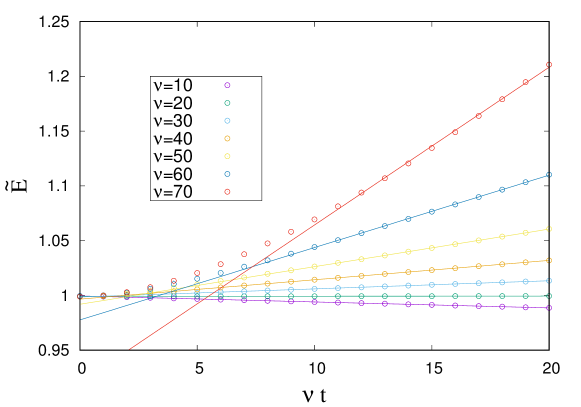
We compare the theoretical result (30) to Monte Carlo simulations of the model in figure 1. This is carried out by fitting $\delta{\tilde{E}}(t)$ with a straight line in the second part of the trajectory, that is, for times long enough so as to the velocity correlations being described by their asymptotic expression (23a) but small as compared to the system size. The agreement is excellent.

There is a critical dissipation value $\nu_{\psi}$ such that $\psi_{\text{\tiny HCS}}$ vanishes, i.e.

$$\nu_{\psi}=\nu_{c}/4=2\pi^{2},\qquad\psi_{\text{\tiny HCS}}(\nu_{\psi})=0,$$ (31)

and the finite-size correction in (30) changes sign. Therefore, at this point we find a change in the time-derivative of $\delta\tilde{E}(t)$. For large system sizes, the energy decays faster (slower) than the Haff law for $\nu<\nu_{\psi}$ ($\nu>\nu_{\psi}$) because $\psi_{\text{\tiny HCS}}<0$ ($\psi_{\text{\tiny HCS}}>0$). In the bottom panel of the figure, we compare the numerical slopes of the rescaled temperature with the theoretical prediction $\psi_{\text{\tiny HCS}}$ as a function of $\nu$. Note that $\psi_{\text{\tiny HCS}}$ diverges as $\nu\to\nu_{c}$, which is a signature of the shear instability of the HCS.

Figure 1: Top panel: rescaled energy $\tilde{E}=1+\delta\tilde{E}$ as a function of time. We compare the numerical values of $1+\delta\tilde{E}$ (circles) and the linear fits (lines) in the second part of the trajectory, for several values of $\nu$ (see legend). Bottom panel: Plot of the slope $m=L\,d\tilde{E}/d(\nu t)$ as a function of $\nu$. We compare the fitted slopes in the top panel (circles) and their theoretical values, as given by $\psi_{\text{\tiny HCS}}$ in (30) (blue line). The transition at $\nu_{\psi}=\nu_{c}/4=2\pi^{2}$ is marked by the horizontal dashed line. We have used a system of size $L=1000$.

4 Beyond Molecular Chaos: Velocity Correlations in the HCS

In this section, we analyse the effect on the free cooling of the system introduced by the velocity correlations. The average equation for the granular temperature (or the energy) in the HCS is closed only when the correlation $\langle v_{l}v_{l+1}\rangle$ is neglected, since it is expected to be of the order of $L^{-1}$. In other words, the evolution equation for the temperature is closed in the Molecular Chaos approximation. Interestingly, for the case of Maxwell molecules we are considering in the paper, we can account for the effect of the correlations in the cooling of the system in quite a detailed way.

4.1 Perturbative Solution for Temperature and Correlations

We assume that the system is in a spatial-translation-invariant state, such as the HCS. We define the set of spatial correlations of the velocity at time $\tau$ as

$$C_{k}(\tau)=\langle v_{j}(\tau)v_{j+k}(\tau)\rangle.$$ (32)

Here, $k$ represents the distance between the involved sites in the correlation. Note that the average temperature at any site $j$ is given by $C_{0}$,

$$T(\tau)\equiv C_{0}(\tau)=\langle v_{j}^{2}(\tau)\rangle.$$ (33)

The evolution equation of these correlations is readily obtained from the master equation,

$$\omega^{-1}\partial_{\tau}{C_{0}} = (\alpha^{2}-1)(C_{0}-C_{1}),$$ (34a)

$$\omega^{-1}\partial_{\tau}{C_{1}} = (1-\alpha^{2})(C_{0}-C_{1})+(1+\alpha)(C_{2}-C_{1}),$$ (34b)

$$\omega^{-1}\partial_{\tau}{C_{k}} = (1+\alpha)(C_{k+1}+C_{k-1}-2C_{k}),\quad 2\leq k\leq(L-1)/2,$$ (34c)

$$\hskip 19.91692ptC_{\frac{L+1}{2}} = C_{\frac{L-1}{2}},\quad\forall\tau.$$ (34d)

In the above equations, we have omitted the $\tau$-dependence of the correlations to keep our notation simple. We have written them for odd $L$, because the “upper” boundary condition (for the maximum value of $k$) is simpler to write. Of course, this choice is irrelevant in the large system size limit.

As a consequence of momentum conservation, in the center of mass frame we have the “sum rule”

$$C_{0}(\tau)+2\sum_{k=1}^{\frac{L-1}{2}}C_{k}(\tau)=0,\quad\forall\tau.$$ (35)

For a conservative ($\alpha=1$) system in equilibrium, the correlations $C_{k}$ do not depend on the distance between sites $k$ and they are of the order $O(L^{-1})$: $C_{k}^{\text{\tiny eq}}=-T(L-1)^{-1}$, $\forall k>0$. In a non-equilibrium state, we may have a non-trivial space structure in the correlations, but we still assume them to be of the order of $L^{-1}$. Then, we define the rescaled correlations $D_{k}(\tau)$ as

$$D_{k}(\tau)=LC_{k}(\tau),$$ (36)

which we assume to be of the order of unity in the infinite size limit as $L\to\infty$.

Let us write (34) in the large system size limit, in which we expect $D_{k}(\tau)$ to be a smooth function of space, in the sense that $D_{k+1}(\tau)-D_{k}(\tau)=O(L^{-1})$. Then, the typical hydrodynamic length and time scales [22] are introduced as

$$x=\frac{k-1}{L},\quad t=\frac{\omega\tau}{L^{2}}.$$ (37)

Keeping solely terms up to $O(L^{-1})$, we arrive at

$$\frac{dT(t)}{dt}=-\nu\left[T(t)-L^{-1}\psi(t)\right],$$ (38a)

$$\nu T(t)+4\partial_{x}{D(x,t)}|_{x=0}=L^{-1}\left(\frac{d\psi(t)}{dt}+\nu\psi(t)\right),$$ (38b)

$$\partial_{t}{D(x,t)}=2\,\partial_{xx}D(x,t),$$ (38c)

$$\partial_{x}{D(x,t)}|_{x=1/2}=\frac{1}{2}L^{-1}\frac{d\chi(t)}{dt}$$ (38d)

in which we have introduced the notations

$$\psi(t)=\lim_{x\rightarrow 0}D(x,t),\quad\chi(t)=\lim_{x\rightarrow\frac{1}{2}}D(x,t).$$ (39)

These equations are exact up to times such that $t\ll L^{2}$, since the lowest order terms that have been neglected are of the order of $L^{-2}$, for instance the fourth-spatial-derivative term in the diffusion equation (38b) for the correlations. In (38a), we have a $L^{-1}$ correction to the cooling rate, brought about by the nearest-neighbour velocity correlation.

Of course, these equations are compatible with the sum rule (35). When we retain only terms up to and including $O(L^{-1})$, we have

$$T(t)+2\int_{0}^{1}dx\,D(x,t)+L^{-1}\left[\psi(t)-2\chi(t)\right]=O(L^{-2}),$$ (40)

as shown in B. The lhs of (40) is a constant of motion, as can be readily shown by using the evolution equations (38).

In order to solve the above system, it is useful to define the scaled (tilde) fields with their corresponding power of $T_{\text{\tiny HCS}}(t)$. Namely, we define

$$\tilde{T}(t)=\frac{T(t)}{T_{\text{\tiny HCS}}(t)},\quad\widetilde{D}(x,t)=\frac{D(x,t)}{T_{\text{\tiny HCS}}(t)}.$$ (41)

These rescaled fields obey the equations

$$\frac{d\tilde{T}(t)}{dt}=\nu L^{-1}\tilde{\psi}(t),$$ (42a)

$$\nu\tilde{T}(t)+4\partial_{x}{\widetilde{D}(x,t)}|_{x=0}=L^{-1}\frac{d\widetilde{\psi}(t)}{dt},$$ (42b)

$$\partial_{t}{\widetilde{D}(x,t)}=\nu\widetilde{D}(x,t)+2\,\partial_{xx}\widetilde{D}(x,t),$$ (42c)

$$\partial_{x}{\widetilde{D}(x,t)}|_{x=1/2}=\frac{1}{2}L^{-1}\left(\frac{d\widetilde{\chi}(t)}{dt}-\nu\widetilde{\chi}(t)\right).$$ (42d)

The system above is linear in $(\tilde{T},\widetilde{D})$, so it is possible to seek the exact solution thereof. In fact, we find the exact solution of the discrete hierarchy (34) in section 5. Here, we are interested in finding the corrections to the cooling rate introduced by the velocity correlations, so we look for a solution of (42) by means of a perturbative approach. This can be performed by expanding all functions of time in powers of $L^{-1}$,

$$\tilde{T}(t)=\tilde{T}_{0}(t)+L^{-1}\tilde{T}_{1}(t)+O(L^{-2}),$$ (43a)

$$\widetilde{D}(x,t)=\widetilde{D}_{0}(x,t)+L^{-1}\widetilde{D}_{1}(x,t)+O(L^{-2}),$$ (43b)

with analogous expansions for $\widetilde{\psi}(t)$ and $\widetilde{\chi}(t)$.
To the lowest order, we have

$$\frac{d}{dt}\tilde{T}_{0}=0,$$ (44a)

$$\nu\tilde{T}_{0}+4\partial_{x}{\widetilde{D}_{0}}|_{x=0}=0,$$ (44b)

$$\partial_{t}{\widetilde{D}_{0}}=\nu\widetilde{D}_{0}+2\,\partial_{xx}\widetilde{D}_{0},$$ (44c)

$$\partial_{x}{\widetilde{D}_{0}}|_{x=1/2}=0.$$ (44d)

From (44a), we have that $\tilde{T}_{0}=1$ is a constant. Moreover, in the limit $t\!\gg\!\!1$, the scaled correlations tend to a stationary value, which is given by

$$\widetilde{D}_{0}(x)=-A\cos\left[\pi\sqrt{\frac{\nu}{\nu_{c}}}(1-2x)\right],\quad A=\pi\sqrt{\frac{\nu}{\nu_{c}}}\csc\left(\pi\sqrt{\frac{\nu}{\nu_{c}}}\right).$$ (45)

Looking for the first order corrections, for our purposes we only need to write the evolution equation for $\tilde{T_{1}}(t)$,

$$\frac{d}{dt}\tilde{T}_{1}(t)=\nu\widetilde{\psi}_{0}(t)$$ (46)

hence when the correlations reached the stationary profile (45) we have that

$$\frac{d}{dt}\tilde{T}_{1}(t)=\nu\psi_{\text{\tiny HCS}}$$ (47)

where $\psi_{\text{\tiny HCS}}$ is the same quantity that we defined in (23) within the mesoscopic fluctuation theory framework, which we rewrite as

$$\quad\psi_{\text{\tiny HCS}}=-\pi\sqrt{\frac{\nu}{\nu_{c}}}\cot\left(\pi\sqrt{\frac{\nu}{\nu_{c}}}\right).$$ (48)

Therefore, for $t\!\gg\!\!1$ the rescaled temperature is linearly diverging as

$$\tilde{T}(t)\sim 1+\frac{\nu\psi_{\text{\tiny HCS}}}{L}t+O(L^{-2})$$ (49)

neglecting the transient terms for $\tilde{T}_{1}$. This result is equivalent to the one in (30) (known that $E(t)=T(t)$ in the homogeneous case) and has been compared with simulations in figure 1.

We have also checked the theoretical prediction (45) for the velocity correlations in the HCS in figure 2. Thus, we plot the simulation value of the amplitude $A$ as a function of $\nu$, and compare it with (45). Trajectories start from a homogeneous mesoscopic velocity profile with zero average, $u(x,0)\equiv 0$. Once more, a very good agreement is found.

Figure 2: Top panel: Time evolution of nearest-neighbour correlations $\psi(t)$. We plot their numerical values (circles) for several $\nu$ (see legend) and $L=1000$ particles as a function of the dimensionless time $\nu t$, and their theoretical stationary values, given by (48). In the plotted time window, the correlations reach their stationary value for all $\nu\leq 60$, while they do not for $\nu=70$. This discrepancy will be analysed in figure 3. Bottom panel: Correlation amplitude $A$, defined in (45), as a function of $\nu$. We plot both its numerical value, computed in simulations for $L=250,500,1000$ (symbols), and its theoretical expectation (black line). A very good agreement is found for all $\nu<70$.

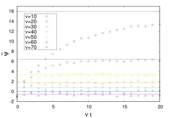
We already commented that the result in (49) is valid only for $\psi_{\text{\tiny HCS}}\nu t/L\ll 1$, while in this section we used the stationary value of the correlations supposing $t\gg 1$. Depending on the value of $\nu$ and $L$, these conditions on time may be either consistent or inconsistent. In fact, numeric data in figure 2 show an excellent agreement with the theoretical prediction in (49) for $\nu<60$, while for higher dissipation the nearest-neighbour correlations do not seem to have reached their stationary value. Therefore, longer trajectories should be observed and this leads to the divergence of the first order perturbation $O(t/L)$.

4.2 Temperature and Correlations Evolution: Multiple-Scale Analysis

In order to build up a theory which give a consistent picture for long times, we introduce a multiple-scale perturbative solution of (42). Equation (42a) suggests the introduction of two distinct time scales: apart from $t$, we define a slow time scale $\sigma$,

$$s=t,\;\sigma=L^{-1}t,\quad\partial_{t}{=}\partial_{s}+L^{-1}\partial_{\sigma}.$$ (50)

Our notation makes it possible to distinguish between $\partial_{t}$ (with constant $x$) and $\partial_{s}$ (with constant $x$ and $\sigma$). All functions of time are expanded in powers of $L^{-1}$ as before and considered to depend on both time scales $(s,\sigma)$. So, to the lowest order we have

$$\partial_{s}{\tilde{T}_{0}}(s,\sigma)=0,$$ (51a)

$$\nu\tilde{T}_{0}+4\partial_{x}{\widetilde{D}_{0}}|_{x=0}=0,$$ (51b)

$$\partial_{s}{\widetilde{D}_{0}}=\nu\widetilde{D}_{0}+2\,\partial_{xx}\widetilde{D}_{0},$$ (51c)

$$\partial_{x}{\widetilde{D}_{0}}|_{x=1/2}=0.$$ (51d)

which has the same form of (44) but now $\tilde{T}_{0}$ depends also on the slow time scale $\sigma$; more precisely, from (51a) we have that it depends only on $\sigma$, $\tilde{T}_{0}(\cancel{s},\sigma)=\tilde{T}_{0}(\sigma)$. Note that $\tilde{T}_{0}(\sigma)$ remains undetermined at the lowest order. Also, (51) leads now to a pseudo-stationary solution for $\widetilde{D}_{0}(x,\cancel{s},\sigma)$ for long time scales $s\gg 1$ but finite $\sigma$, namely

$$\widetilde{D}_{0}(x,\sigma)=-\tilde{T}_{0}(\sigma)A\cos\left[\pi\sqrt{\frac{\nu}{\nu_{c}}}(1-2x)\right],$$ (52)

which differs from (45) because of the $\sigma$ dependence of $\tilde{T}_{0}(\sigma)$. As is usual in multiple-scale analysis, the latter can be obtained by writing down the equations for the first order corrections. In fact, for the purposes of the present paper, it suffices to write the evolution equation for $T_{1}(s,\sigma)$,

$$\partial_{s}{\tilde{T}}_{1}+\frac{d}{d\sigma}{\tilde{T}_{0}}=\nu\widetilde{\psi}_{0},\qquad\widetilde{\psi}_{0}=\tilde{T}_{0}\psi_{\text{\tiny HCS}}.$$ (53)

Since the rescaled energy should not contain linear terms in time (see section 5 for a rigorous proof), the first lhs term of (53) must vanish, and

$$\nu\psi_{\text{\tiny HCS}}\tilde{T}_{0}(\sigma)-\frac{d}{d\sigma}{\tilde{T}_{0}}=0\;\Rightarrow\;\tilde{T}_{0}(\sigma)=e^{\nu\psi_{\text{\tiny HCS}}\sigma},$$ (54)

where we have taken into account that $\tilde{T}_{0}(t=0)=1$. Going back to the unscaled variables, what we have shown is that

$$T(t)=T(0)\exp\left[-\nu_{\text{\tiny HCS}}^{r}t\right]+O(L^{-1}),\qquad\nu_{\text{\tiny HCS}}^{r}=\nu\left(1-L^{-1}\psi_{\text{\tiny HCS}}\right).$$ (55)

Equation (55) tells us that the cooling rate in Haff’s law has a finite size correction. Of course, if we consider that $\sigma=t/L\ll 1$ and retain only the linear terms in $L^{-1}$, we reobtain the results in section 3 and in (49).

Figure 3: Top panel: Log-linear plot of the rescaled temperature. The simulation values are plotted for $\nu=50,60,70$ (circles), and also the fits made upon the second part of the long trajectories (lines). The time evolution is clearly exponential as predicted from (54). Inset: Time evolution of the nearest-neighbour correlations $\psi(t)$ for long trajectories. We have plotted the simulation curves (circles) and their corresponding theoretical stationary values (lines). Bottom panel: Slope $m_{l}$ of the time evolution of $\ln\tilde{T}$. The fitting values from the top panel (squares) are plotted together with the theoretical prediction (54) (black line). All the trajectories have been done with $L=1000$ particles up to a maximum time $\nu t=200$.

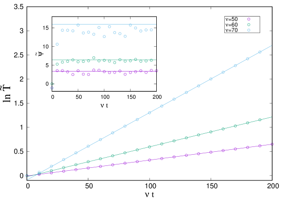
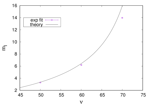
We check the renormalisation of Haff’s law predicted by (55) in figure 3: simulations made over long times $\nu t\psi_{\text{\tiny HCS}}\sim L$ show that the rescaled temperature has an exponential behaviour, as predicted from the multiple-scale analysis. The exponential slope has been fitted and numerical results are in good agreement with the theoretical prediction (54). Nearest-neighbour correlations have been studied as before: figure 3 shows that for $\nu=50,60$ they converge to their expected value after a very short transient, whereas for $\nu=70$ they also converge but to a stationary value smaller than the expected one. This effect is probably given by next order corrections which are becoming relevant when approaching the critical dissipation $\nu_{c}$, where we know that $\psi_{\text{\tiny HCS}}$ is divergent.

5 Exact solution of the HCS in a finite system

The hierarchy (34) can be exactly solved by reducing it to the eigenvalue problem of a certain matrix. As before, we carry out this approach to the problem for odd $L$; a choice that is irrelevant in the large system size limit $L\gg 1$. The problem for an even number particles may be solved by following an utterly similar strategy, but the boundary conditions are a little more involved to write. We do not present here these calculations because they do not provide any additional physical insight.

First, it is useful to introduce a change of variables in order to make the matrix symmetric. Specifically, we define

$$c_{0}=C_{0},\qquad c_{k}=\sqrt{2}\,C_{k},\quad 1\leq k\leq(L-1)/2.$$ (56)

Second, we rewrite the hierarchy (34) as

$$\hskip 8.53581pt\omega^{-1}(1+\alpha)^{-1}\partial_{\tau}c_{0} = -(1-\alpha)c_{0}+\frac{1-\alpha}{\sqrt{2}}c_{1},$$ (57a)

$$\hskip 8.53581pt\omega^{-1}(1+\alpha)^{-1}\partial_{\tau}c_{1} = \frac{1-\alpha}{\sqrt{2}}c_{0}-\frac{3-\alpha}{2}c_{1}+c_{2},$$ (57b)

$$\hskip 8.53581pt\omega^{-1}(1+\alpha)^{-1}\partial_{\tau}c_{k} = c_{k-1}-2c_{k}+c_{k+1},\quad 2\leq k\leq(L-3)/2,$$ (57c)

$$\omega^{-1}(1+\alpha)^{-1}\partial_{\tau}c_{\frac{L-1}{2}} = c_{\frac{L-3}{2}}-c_{\frac{L-1}{2}},$$ (57d)

in which we have extracted the common factor $(1+\alpha)$ on the rhs of (34) and made use of (34d) to write (57d) for $c_{\frac{L-1}{2}}$.

Now, we can solve the system above by a standard eigenvector method, that is, we seek solutions of the form

$$c_{k}=e^{\lambda(1+\alpha)\omega\tau}\phi_{k}.$$ (58)

We denote the eigenvalues by $\lambda$ and its corresponding eigenvector by $\phi$, $\phi_{k}$ is thus the $k$-th component thereof. In this way, we reach the system

$$\hskip 8.53581pt\lambda\phi_{0} = -(1-\alpha)\phi_{0}+\frac{(1-\alpha)}{\sqrt{2}}\phi_{1},$$ (59a)

$$\hskip 8.53581pt\lambda\phi_{1} = \frac{(1-\alpha)}{\sqrt{2}}\phi_{0}-\frac{(3-\alpha)}{2}\phi_{1}+\phi_{2},$$ (59b)

$$\hskip 8.53581pt\lambda\phi_{k} = \phi_{k-1}-2\phi_{k}+\phi_{k+1},\quad 2\leq k\leq(L-3)/2,$$ (59c)

$$\lambda\phi_{\frac{L-1}{2}} = \phi_{\frac{L-3}{2}}-\phi_{\frac{L-1}{2}}.$$ (59d)

Equations (59) are a system of second-order difference equations for $\phi_{k}$ with contant coefficients, in which (59c) is the general equation and (59b) and (59d) are their boundary conditions. On top of that, (59a) acts as an extra condition that ensures momentum conservation, as shown below (see also section 4). The general solution of (59c) is of the form $\phi_{k>0}=r^{k}$ [25], which substituted into (59c) has two solutions $(r_{1},r_{2})$ that verify

$$r_{1}r_{2}=1,\qquad r_{1}+r_{2}=2+\lambda.$$ (60)

We introduce a new variable $q\in[0,\pi]$ such that $r_{1}=e^{iq}$ and $r_{2}=e^{-iq}$, as suggested by (60). Note that $|r_{1}|=|r_{2}|=1$, if one of the roots were larger than one it would lead to correlations increasing with $k$, which is physically absurd. Moreover, from a purely mathematical point of view, restricting ourselves to $|r_{1}|=|r_{2}|=1$ leads to a complete set of eigenvectors. From (60), we obtain

$$\lambda(q)=2(\cos q-1),$$ (61)

and the corresponding eigenvector is given by

$$\phi_{k>0}(q) = A\,e^{ikq}+B\,e^{-ikq},$$ (62a)

$$\hskip 8.53581pt\phi_{0}(q) = \frac{1-\alpha}{\sqrt{2}\left(2\cos q-1-\alpha\right)}(A\,e^{iq}+B\,e^{-iq}).$$ (62b)

The boundary conditions (59b) and (59d) determine the constants $A$ and $B$, and also the allowed values of the “index” $q$. The determinant of the linear system for $A$ and $B$ must be zero, which is equivalent to impose that $q$ must be a zero of the function

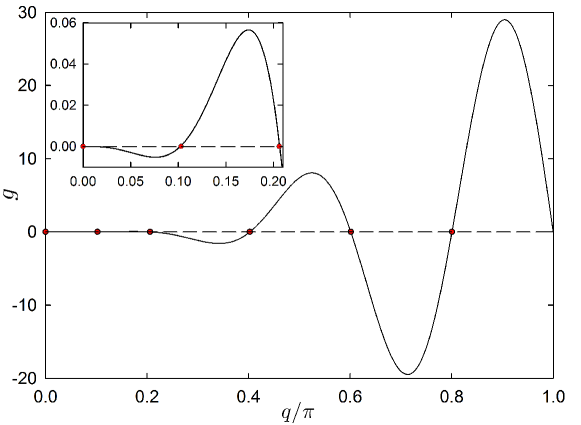
$$g(q)= 2\sin\left(\frac{L+3}{2}q\right)-(5+3\alpha)\sin\left(\frac{L+1}{2}q\right)+(5+7\alpha)\sin\left(\frac{L-1}{2}q\right)$$ (63)

$$-(3+5\alpha)\sin\left(\frac{L-3}{2}q\right)+(1+\alpha)\sin\left(\frac{L-5}{2}q\right).$$

This function has $(L+1)/2$ different zeros in the half-open interval $[0,\pi)$, which we denote by $q_{n}$: $q_{0}=0$, $q_{n}$ is the $n$-th non-vanishing zero of $g(q)$, $n=1,\ldots,(L-1)/2$. Therefore, we have found $(L+1)/2$ eigenvalues

$$\lambda_{n}=2(\cos q_{n}-1),$$ (64)

the corresponding eigenvectors of which give a complete set for the problem at hand. In figure 4 we plot the function $g(q)$ for $L=11$, which has six zeros in the interval $[0,\pi)$.

Figure 4: Plot of the function $g(q)$ defined in (63) for $L=11$. The zeros $q_{n}$ of this function determine the eigenvalues, by taking into account (64). The first zero is always $q_{0}=0$, and there are $(L-1)/2$ non-vanishing zeros $q_{i}$, $i=1,\ldots,(L-1)/2$. A zoom of the small $q$ region is shown in the inset, in order to make it easier the identification of $q_{1}$ and $q_{2}$.

The eigenvector $\phi^{(n)}$ corresponding to the eigenvalue $\lambda_{n}$ can be thus written up to a normalisation constant $\mathcal{N}_{n}$,

$$\phi^{(n)}_{k>0} = \mathcal{N}_{n}\cos\left[\left(\frac{L}{2}-k\right)q_{n}\right],$$ (65a)

$$\phi^{(n)}_{0} = \frac{(1-\alpha)\mathcal{N}_{n}}{\sqrt{2}\left(2\cos q_{n}-1-\alpha\right)}\cos\left[\left(\frac{L}{2}-1\right)q_{n}\right].$$ (65b)

The above expressions clearly show that there is no eigenvector for $q=\pi$, since all its components are zero (recall that $L$ is odd). The constant $\mathcal{N}_{n}$ is chosen to obtain a orthonormal set of eigenvectors, in the sense that

$$\sum_{k=0}^{\frac{L-1}{2}}\phi^{(n)}_{k}\phi^{(n^{\prime})}_{k}=\delta_{nn^{\prime}}.$$ (66)

We do not give the explicit expression for $\mathcal{N}_{n}$ because it is quite involved and is not necessary for our purposes. The eigenvector corresponding to $q_{0}=0$ is particularly simple, (65) implies that

$$\phi_{0}^{(0)}=\frac{\mathcal{N}_{0}}{\sqrt{2}},\quad\phi_{k>0}^{(0)}=\mathcal{N}_{0},\qquad\mathcal{N}_{0}=\sqrt{\frac{2}{L}}.$$ (67)

Then, the orthogonality relation of $\phi^{(0)}$ and $\phi^{(n)}$ ($n\neq 0$) makes it possible to write a “sum rule” for the components of the latter eigenvectors,

$$\phi_{0}^{(n)}+\sqrt{2}\sum_{k=1}^{\frac{L-1}{2}}\phi_{k}^{(n)}=0,\quad n>0.$$ (68)

This sum rule is connected with  (35), which stemmed from momentum conservation. It also allows us to write $\phi_{0}^{(n)}$ in a more convenient form for some calculations,

$$\phi_{0}^{(n)}=-\frac{\mathcal{N}_{n}}{\sqrt{2}}\csc\left(\frac{q_{n}}{2}\right)\sin\left(\frac{L-1}{2}q_{n}\right),$$ (69)

which does not depend explicitly on $\alpha$.

Finally, we have all the ingredients to build the general solution of (57) as the sum

$$c_{k}=\sum_{n=1}^{\frac{L-1}{2}}a_{n}\,e^{\lambda_{n}(1+\alpha)\omega\tau}\phi_{k}^{(n)},$$ (70)

where $a_{n}$ is given in terms of the initial conditions by

$$a_{n}=\sum_{k=0}^{\frac{L-1}{2}}\phi_{k}^{(n)}c_{k}(0).$$ (71)

The sum in (70) starts from $n=1$ because $a_{0}=0$, since

$$a_{0}=\mathcal{N}_{0}\left[\frac{c_{0}(0)}{\sqrt{2}}+\sum_{k=1}^{\frac{L-1}{2}}c_{k}(0)\right]=\frac{\mathcal{N}_{0}}{\sqrt{2}}\left[C_{0}(0)+2\sum_{k=1}^{\frac{L-1}{2}}C_{k}(0)\right]=0.$$ (72)

We have made use of momentum conservation, as expressed by the sum rule (35), in the last equality.

5.1 Eigenvalues for large systems

Here, we would like to derive an approximate expression for the eigenvalue spectrum in the large system size limit $L\gg 1$. Therefore, we consider that the microscopic dynamics is quasi-elastic by introducing the macroscopic dissipation coefficient $\nu$, $(1-\alpha^{2})L^{2}=\nu$, as in (8). The eigenvalues are given by the zeros of function (63), and we expand this function for $q\ll 1$ by introducing the scaling $Q=qL$, with the result

$$\tan\left(\frac{Q}{2}\right)\left(\frac{\nu}{2}Q^{2}L^{-2}-Q^{4}L^{-4}\right)+\frac{1}{2}Q^{5}L^{-5}=0.$$ (73)

We are assuming that $Q$ is of the order of unity and have neglected terms of the order of $L^{-6}$.

In order to obtain an analytical approximation for the eigenvalues, we propose an expansion of $Q_{n}=q_{n}L$ in powers of $L^{-1}$, $Q_{n}=Q^{(0)}_{n}+Q^{(1)}_{n}L^{-1}+O(L^{-2})$. To the lowest order, we obtain

$$Q^{(0)}_{1} = \sqrt{\frac{\nu}{2}},$$ (74a)

$$Q^{(0)}_{n} = 2(n-1)\pi,\qquad n=2,\ldots,(L-1)/2.$$ (74b)

Moreover, the finite size corrections are

$$Q^{(1)}_{1} = \frac{\nu}{8\tan\left(\frac{1}{2}\sqrt{\frac{\nu}{2}}\right)},$$ (75a)

$$Q^{(1)}_{n} = \frac{16(n-1)^{3}\pi^{3}}{8(n-1)^{2}\pi^{2}-\nu},\qquad n=2,\ldots,(L-1)/2.$$ (75b)

Note that $Q_{1}^{(1)}$ vanishes at $\nu=\nu_{\psi}=2\pi^{2}$ whereas it diverges at $\nu=\nu_{c}=8\pi^{2}$. The former property is connected to the change of sign in the finite-size correction to the cooling rate of the HCS whereas the latter gives rise to the instability of the HCS, as discussed in sections 3 and 4.

Figure 5: Plot of the difference $Q_{1}-Q_{1}^{(0)}$ as a function of the system size $L$. Three different values of the macroscopic dissipation coefficient $\nu$ are considered, namely $\nu=\pi^{2}$, $\nu=\nu_{\psi}=2\pi^{2}$ and $\nu=4\pi^{2}$. Two curves are shown for each value of $\nu$: the lines correspond to the theoretical curve $Q_{1}^{(1)}/L$ and the symbols to the numerical estimate of $Q_{1}$ (see the legend for details). It is clearly observed that the finite-size correction is especially small for $\nu=\nu_{\psi}$.

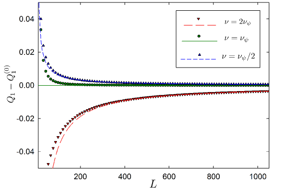
In figure 5, we check the above expansion for the zeros of the function $g(q)$. Specifically, we do so for the first zero $q_{1}$: the numerical estimation of $q_{1}$ is compared with the expansion in (74) and (75) by plotting $Q_{1}-Q_{1}^{(0)}$ as a function of the system size $L$. It is observed that this difference tends to zero as the system size increases, for all the considered values of $\nu$. The finite size correction is especially small for $\nu=\nu_{\psi}=2\pi^{2}$, for which the theoretical correction $Q_{1}^{(1)}$ vanishes. Therefore, finite size corrections are as small as possible for this case, which makes it particularly adequate to investigate the hydrodynamic description, as done in [21, 22].

We want to emphasise that the instability of the HCS is reobtained here as a crossing between the first two non-zero eigenvalues: for $\nu=\nu_{c}=8\pi^{2}$, we have that $Q_{1}^{(0)}=Q_{2}^{(0)}$. On the one hand, for $\nu<\nu_{c}$, the largest nonvanishing eigenvalue is $\lambda_{1}$ ($\lambda_{1}<0$) and dominates the long-time dynamics of the system: the energy $C_{0}$ and all the correlations $C_{k}$ decay with $\exp[\lambda_{1}\omega(1+\alpha)\tau]=\exp(\nu_{\text{\tiny HCS}}^{r}t)$, see below. On the other hand, for $\nu>\nu_{c}$, the dominant term is the one corresponding to $Q_{2}\simeq 2\pi$ and the long time behaviour of the system becomes independent of $\nu$.

The large system size limit of the eigenvalues is then

$$\lambda_{n}=-\frac{{Q_{n}^{(0)}}^{2}}{L^{2}}\left[1+L^{-1}\frac{2Q_{n}^{(1)}}{Q_{n}^{(0)}}+O(L^{-2})\right].$$ (76)

Moreover, the exponent in (70) controlling the time dependence of the contribution for each mode is

$$\lambda_{n}(1+\alpha)\omega\tau \sim -2{Q_{n}^{(0)}}^{2}\left[1+L^{-1}\frac{2Q_{n}^{(1)}}{Q_{n}^{(0)}}+O(L^{-2})\right]t,$$ (77)

which shows the relevance of the hydrodynamic scale $t$ in the large system size limit.

5.2 Long time limit

Equation (70) gives the general time evolution for the velocity correlations. Here, we show that these correlations tend to their HCS values in the long time limit, provided that $\nu<\nu_{c}$, that is, we are below the instability.

Let us consider the scaled correlations $\tilde{C}_{k}$

$$\tilde{C}_{k}(\tau)=\frac{C_{k}(\tau)}{C_{0}(\tau)}=\frac{c_{k}(\tau)}{\sqrt{2}c_{0}(\tau)},$$ (78)

i.e., we scale the correlations with the energy $C_{0}\neq 0$. For long enough times, the only relevant contribution to (70) stems from the maximum (minimum in absolute value) eigenvalue $\lambda_{1}$. Thus, the time dependence for all the correlations $C_{k}$ (or $c_{k}$) are the same and, consequently, the quotient in (78) becomes time-independent for long enough times. Making use of (70) and (69),

$$\tilde{C}_{k}=\frac{\phi^{(1)}_{k}}{\sqrt{2}\phi^{(1)}_{0}}=-\sin\left(\frac{q_{1}}{2}\right)\csc\left(\frac{L-1}{2}q_{1}\right)\cos\left[\left(\frac{L}{2}-k\right)q_{1}\right],$$ (79)

which is nothing but the discrete version of (45).

We can also derive the rate at which the energy and all the correlations are decaying in the long time limit. Particularising (77) for $n=1$, we have that

$$\lambda_{1}(1+\alpha)\omega\tau\sim-\nu t\left[1-L^{-1}\psi_{\text{\tiny HCS}}+O(L^{-2})\right]=-\nu_{\text{\tiny HCS}}^{r}t,$$ (80)

where $\nu_{\text{\tiny HCS}}^{r}$ is the “renormalised” by fluctuations cooling rate introduced in (55) after a multiple scale analysis of the finite size corrections to the hydrodynamic description. The energy is given by $C_{0}(t)=T(t=0)\exp(-\nu_{\text{\tiny HCS}}^{r}t)$ and the correlations $C_{k}$ follow from (79).

6 Total energy fluctuations and multiscaling

A typical question in granular systems concerns the distribution of the extensive energy ${\cal K}(\tau)=\sum_{l}v^{2}_{l}(\tau)$: usually, granular models present non-Gaussian distributions that can be mostly characterized by the study of its fluctuations [24]. Within the same spirit of section 4.1, we now aim to derive the total energy rescaled fluctuations $\Sigma(\tau)$ defined as

$$\Sigma^{2}(\tau)=\frac{\left\langle{\cal K}^{2}(\tau)\right\rangle-\left\langle{\cal K}(\tau)\right\rangle^{2}}{\left\langle{\cal K}(\tau)\right\rangle^{2}}.$$ (81)

The Local Equilibrium Approximation (LEA) gives the straightforward result $\Sigma^{2}(\tau)=2/L$. However, numerical results in figure 6 show a time-dependent behaviour of $\Sigma^{2}(\tau)$ which clearly diverges from the LEA prediction.

Figure 6: Total energy rescaled fluctuations as a function of dimensionless time $\nu t$. We have plotted the simulation curves for $\nu=10,20,\ldots,70$, always with $L=1000$. The divergence from the expected LEA value is evident and grows with $\nu$.

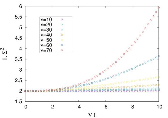
Such anomalous behaviour is generally considered an evidence of multiscaling in the moments [26], i.e. the moments are not scaling proportionally to the granular temperature $T(\tau)=\left\langle v^{2}(\tau)\right\rangle$. Notwithstanding, this phenomenon can also be explained by a well-defined scaled distribution function with some divergent moments [27, 28]. Following the same approach of section 4.1, we look for a direct calculation of the energy fluctuations by means of the evolution equations for the $4$-th order moments and correlations.

In the homogeneous case, we can write

$$\left\langle{\cal K}^{2}(\tau)\right\rangle = \sum^{L}_{l=1}\left\langle v^{4}_{l}(\tau)\right\rangle+\sum^{L}_{l=1}\sum^{L-1}_{k=1}\left\langle v^{2}_{l}(\tau)\,v^{2}_{l+k}(\tau)\right\rangle$$ (82a)

$$= L\left\langle v^{4}(\tau)\right\rangle+L\left[(L-1)T^{2}(\tau)+2\sum^{(L-1)/2}_{k=1}C^{2,2}_{k}(\tau)\right],$$

$$\hskip 8.53581pt\left\langle{\cal K}(\tau)\right\rangle = LT(\tau),$$ (82b)

where we have defined the two-particle squared velocity correlation function

$$C^{2,2}_{k}(\tau)=\left\langle v^{2}_{l}(\tau)v^{2}_{l+k}(\tau)\right\rangle-T^{2}(\tau),\quad k\neq 0.$$ (83)

Therefore, the energy fluctuations dynamics is given by the dynamics of $T(\tau)$, $q(t)=\left\langle v^{4}(t)\right\rangle$ and $C^{2,2}_{k}(\tau)$ altogether.

Rescaled energy fluctuations hence read

$$L\Sigma^{2}(t)=2+a_{2}(t)+\frac{2}{T^{2}(t)}\int_{0}^{\frac{1}{2}-\frac{3}{2L}}D^{2,2}(x,t)dx,$$ (84)

using the hydrodynamic scaling defined in (37) and introducing the excess kurtosis field $a_{2}(t)=q(t)/T^{2}(t)-3$. Analogously with the scaling used in section 4, we define $D^{2,2}=LC^{2,2}$, where the evolution equations for these fields can be computed from the microscopic dynamics (2). By means of a perturbative approach, a set of equations is derived, similar to (44), coupling all the one-particle and two-particle fourth-degree fields, namely $q(t)$, $D^{2,2}(x,t)$ and $D^{3,1}(x,t)$. The latter is the large-size limit of $D^{3,1}_{k}(\tau)=L\left\langle v^{3}_{l}(\tau)\,v_{l+k}(\tau)\right\rangle$. Also, the three-particle correlation $C^{1,2,1}_{i,j}(\tau)=\left\langle v_{l-i}(\tau)\,v^{2}_{l}(\tau)\,v_{l+j}(\tau)\right\rangle$ appears in these equations: to get a closed set, we make use of the clustering ansatz, that is, we perform a cluster expansion of the latter and neglect purely correlated terms, specifically

$$C^{1,2,1}_{i,j}(\tau) = \left\langle v^{2}_{l}(\tau)\right\rangle\left\langle v_{l-i}(\tau)\,v_{l+j}(\tau)\right\rangle+2\left\langle v_{l}(\tau)\,v_{l-i}(\tau)\right\rangle\left\langle v_{l}(\tau)\,v_{l+j}(\tau)\right\rangle$$

$$+\mathcal{O}(L^{-3})=\frac{1}{L}T(\tau)D_{|i+j|}(\tau)+\frac{2}{L^{2}}D_{i}(\tau)D_{j}(\tau)+\mathcal{O}(L^{-3}).$$

Using the microscopic dynamics defined in (2) and moving to the continuum limit defined in section 4, with the clustering ansatz one gets to the lowest order

$$\frac{d}{dt}\tilde{q}_{0}(t)=0,$$ (86a)

$$\nu\left[\tilde{q}_{0}(t)+3\tilde{T}^{2}_{0}\right]+8\partial_{x}{\widetilde{D}^{3,1}_{0}}|_{x=0}=0,$$ (86b)

$$\partial_{t}{\widetilde{D}^{3,1}_{0}}=\frac{\nu}{2}\left(\widetilde{D}^{3,1}_{0}+\tilde{T}_{0}\widetilde{D}_{0}\right)+2\,\partial_{xx}\widetilde{D}^{3,1}_{0},$$ (86c)

$$\partial_{x}{\widetilde{D}^{3,1}_{0}}|_{x=1/2}=0,$$ (86d)

$$\partial_{x}{\widetilde{D}^{2,2}_{0}}|_{x=0}=0,$$ (86e)

$$\partial_{t}{\widetilde{D}^{2,2}_{0}}=2\,\partial_{xx}\widetilde{D}^{2,2}_{0},$$ (86f)

$$\partial_{x}{\widetilde{D}^{2,2}_{0}}|_{x=1/2}=0.$$ (86g)

These equations can be readily solved. Assuming for instance the initial distribution to be Gaussian, we have at any time $\tilde{q}_{0}=3\,\tilde{T}^{2}_{0}$. Moreover, in the long time limit $t\gg 1$, we obtain the stationary fields

$$\widetilde{D}^{3,1}_{0}(x)=3\,\widetilde{D}_{0}(x),\qquad\widetilde{D}^{2,2}_{0}(x)=0,$$ (87)

recalling that $\tilde{T}_{0}=1$. However, these results do not give rise to any multiscaling effect such as the one observed into the simulations.

In light of the above, we move on to compute the next perturbative order. The equations needed from the definition (84) are those for $\tilde{q}_{1}$ and $\widetilde{D}^{2,2}_{1}$, i.e.

$$\frac{d}{dt}\tilde{q}_{1}(t)=2\nu\psi^{3,1}_{0}(t),$$ (88a)

$$\nu\tilde{T}_{0}\tilde{\psi}_{0}+\partial_{x}{\widetilde{D}^{2,2}_{1}}|_{x=0}=0,$$ (88b)

$$\partial_{t}{\widetilde{D}^{2,2}_{1}}=2\,\partial_{xx}\widetilde{D}^{2,2}_{1}+4\,\nu\tilde{D}^{2}_{0},$$ (88c)

$$\partial_{x}{\widetilde{D}^{2,2}_{1}}|_{x=1/2}=0.$$ (88d)

Equation (88a) is immediately solvable for long times since $\tilde{D}^{3,1}_{0}(x,t)$ is known from (87), yielding

$$\tilde{q}_{1}(t)=2\nu\psi^{3,1}_{0}=6\nu\psi{\text{\tiny HCS}}.$$ (89)

Looking at the $\tilde{D}^{2,2}_{1}$ field from (84), all we need is to compute the integral $\Delta_{1}(t)=\int^{1}_{0}dx\,\tilde{D}^{2,2}_{1}(x,t)$. Taking into account (88), we have that

$$\frac{d}{dt}\Delta_{1}(t)=4\nu\left[\psi_{0}(t)+\int^{1}_{0}dx\,\widetilde{D}^{2}_{0}(x,t)\right],$$ (90)

where we have used the boundary condition $\partial_{x}{\widetilde{D}^{2,2}_{1}}|_{x=1^{-}}=-\partial_{x}{\widetilde{D}^{2,2}_{1}}|_{x=0^{+}}$. Therefore, in the long time limit we use the stationary correlation profile $\widetilde{D}(x)$ from (45) to get the stationary growth

$$\frac{d}{dt}\Delta_{1}(t)=2\nu\left[\frac{\pi\sqrt{\nu/\nu_{c}}}{\sin\left(\pi\sqrt{\nu/\nu_{c}}\right)}\right]^{2}\left[1-\frac{\sin\left(2\pi\sqrt{\nu/\nu_{c}}\right)}{2\pi\sqrt{\nu/\nu_{c}}}\right].$$ (91)

Now, we have all the ingredients to compute the energy fluctuations in (84). To the first order, (89) and (46) yield that the excess kurtosis $a_{2}(t)$ vanishes for all times if it did initially, $a_{2}(t)=O(L^{-2})$. This implies that the steady-state linear divergence of the energy fluctuations (to the first order) is given by the $D^{2,2}$ correlations term in (91). Specifically, for $t\gg 1$, we have

$$\frac{d}{dt}\Sigma^{2}(t)=\frac{1}{L}\frac{d}{dt}\Delta_{1}(t)=\frac{\nu}{L}m_{\Sigma}(\nu).$$ (92)

We have introduced $m_{\Sigma}(\nu)=d\Delta_{1}/d(\nu t)$, which is the slope of the energy fluctuations as a function of the dimensionless time $\nu t$.

In conclusion, the observed energy multiscaling seems to stem from the multiscaling of many-particle correlation fields, while the single-particle fourth moment still scales with the granular temperature squared. We have compared this theoretical result with simulations in figure 7. Although some discrepancies are apparent, especially for high $\nu$, we see that they both exhibit a similar trend over three decades of $m_{\Sigma}$ values.

Figure 7: Slope of the energy fluctuations vs. time curves. We compare the fitted values (symbols) in the second part (long time) of the trajectories for $L=250,500,1000$ with the theoretical prediction $m_{\Sigma}(\nu)$ in (92) (black line). Simulations are carried out as in figure 6.

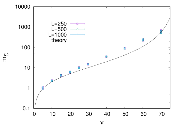
Keeping the clustering ansatz in (6), a multiple scale analysis has also been performed, analogous to that in section 4. Nevertheless, it does not improve the agreement with the numerics. Therefore, it seems that the most probable source for this discrepancy is the clustering ansatz that is used in both cases.

7 Conclusions

We have followed different approaches to obtain the long-range correlations in a 1d lattice model for the velocity and energy fields of a granular gas. The most compact approach takes advantage of a fluctuating hydrodynamic description: it reproduces the fluctuations and correlations of the shear-modes already known in the homogeneous cooling of inelastic hard-spheres [29]. In addition, it gives an approximate value of the finite-size correction to the Haff-law describing the decay of the energy.

Fluctuating hydrodynamics however involves a continuum limit that implies the appearance of irregular fields, a problem which is known in the literature [30]. On the one hand, the results of fluctuating hydrodynamics can be reproduced and improved through the study of correlations before taking the continuum limit. On the other hand, still within this framework, a multiple scale analysis makes it possible to derive the renormalisation of the cooling rate in a more consistent way.

An exact treatment of the hierarchy of equations for the two-particle correlations gives access to the eigenvalue spectrum for their time evolution. Of course, this approach reproduces the continuum limit results when a large system is considered, and it is useful to understand how the continuum limit emerges and the different timescales that are relevant in the system. Both the energy $C_{0}=\langle v_{l}^{2}\rangle$ and all the velocity correlations $C_{k}=\langle v_{l}v_{l+k}\rangle$ tend to zero in the long time limit as a consequence of the cooling, but the scaled correlations $C_{k}/C_{0}$ become time-independent. Therefore, the system ends up in the HCS, independently of the initial preparation.

The above study also improves our understanding of the shear instability in the HCS, as it comes about as a crossing between the first two exact eigenvalues of the problem. Also, it improves our understanding of the situation beyond the instability ($\nu>\nu_{c}$) in the present model: we find that both the energy and the correlations still decay to zero but with a rate that is independent of the inelasticity. Note that our system cannot develop inhomogeneities in the density because particles are fixed.

In addition, we have also observed numerically an unexpected multiscaling phenomenon at finite size. While one-particle moments scale with their corresponding power of the granular temperature, some multiple-particle moments do not. This implies that the variance of the total energy departs from its “simple” scaled value as time increases, with an approximate constant slope that seems to diverge close to the shear instability. We have developed a theoretical approach, based on a clustering hypothesis for three-particle moments, that predicts this multiscaling behaviour. However, the agreement between the theory and the simulation is not perfect, probably as a consequence of the clustering approximation.

An interesting future challenge is to adapt the framework of the Macroscopic Fluctuation Theory [11, 30] to our model. In its present state, the theory does not deal with macroscopic equations with advection terms and momentum conservation, such as those in the Navier-Stokes equations that inevitably appear in granular hydrodynamics. Our model, which enforces momentum conservation but neglects advection, represents a possible bridge toward this goal.

Appendix A Fluctuating expression for the dissipation

Let us consider the dissipation $d_{l,p}$ at site $l$ and at time $p$. Its main part is obtained by averaging (4) with respect to the fast variables $y_{l,p}$, i.e.

$$\bar{d}_{l,p}=\frac{\alpha^{2}-1}{4L}\left(\Delta_{l,p}^{2}+\Delta_{l-1,p}^{2}\right)<0.$$ (93)

This is the expression that we have to analyse in the fluctuating hydrodynamic description, since the amplitude of the dissipation noise scales as $L^{-3}$. If we consider the average of the dissipation field, it is readily obtained that $d^{\text{av}}_{l,p}=(\alpha^{2}-1)T_{l,p}/L$, which gives (8) in the continuum limit by using $d(x,t)=L^{3}d_{l,p}$ and the definition of $\nu$. Therefore, it is consistent to write at the fluctuating level that

$$\bar{d}_{l,p}=\frac{\alpha^{2}-1}{L}\theta_{l,p},$$ (94)

by defining the fluctuating temperature as

$$\theta_{l,p}=\frac{1}{4}\left(\Delta_{l,p}^{2}+\Delta_{l-1,p}^{2}\right)=\frac{v_{l-1,p}^{2}+2v_{l,p}^{2}+v_{l+1,p}^{2}}{4}-v_{l,p}\frac{v_{l+1,p}+v_{l-1,p}}{2}.$$ (95)

The first term on the rhs, $(v_{l-1,p}^{2}+2v_{lp}^{2}+v_{l+1,p}^{2})/4$, reduces to $e_{l,p}$ plus terms of the order of $L^{-2}$, which are neglected.

Our main goal in to obtain a correct expression for $v_{l,p}v_{l\pm 1,p}$ at the fluctuating level. In general, we have for the average correlations

$$\langle v_{l,p}v_{l^{\prime},p}\rangle=E_{l,p}\delta_{ll^{\prime}}+C_{l,l^{\prime}-l;p}\left(1-\delta_{ll^{\prime}}\right),$$ (96)

with the definition

$$C_{l,l^{\prime}-l;p}=\langle v_{l,p}v_{l^{\prime},p}\rangle\quad\text{for $l^{\prime}\neq l$}.$$ (97)

The functions $C_{k,p}$ defined in section 4 are the particularisation of $C_{l,l^{\prime}-l;p}$ to an homogeneous situation ($k=l^{\prime}-l$). Consistently with (96), we write

$$v_{l,p}v_{l^{\prime},p}=e_{l,p}\delta_{ll^{\prime}}+\gamma_{l,l^{\prime}-l,p}\left(1-\delta_{ll^{\prime}}\right)=\gamma_{l,l^{\prime}-l,p}+\left(e_{l,p}-\gamma_{l,l^{\prime}-l,p}\right)\delta_{ll^{\prime}},$$ (98)

at the fluctuating level. We have introduced the fluctuating correlations $\gamma_{l,l^{\prime}-l,p}$, such that $\langle\gamma_{l,l^{\prime}-l;p}\rangle=C_{l,l^{\prime}-l,;p}$. In the continuum limit, $x=l/L$ and $x^{\prime}=l^{\prime}/L$ and (98) is transformed into

$$v(x,t)v(x^{\prime},t)=\gamma(x,x^{\prime}-x;t)+L^{-1}\delta(x-x^{\prime})\left[e(x,t)-\gamma(x,x^{\prime}-x;t)\right],$$ (99)

because $\delta_{l,l^{\prime}}\sim L^{-1}\,\delta(x-x^{\prime})$ (see note at the end of the appendix).

Taking into account (95) and the above definitions, the fluctuating temperature in the continuum limit is

$$\theta(x,t)=e(x,t)-\gamma(x,0;t),$$ (100)

where we have neglected terms of the order of $L^{-2}$. Since we are interested in the limit of $\gamma(x,\Delta x;t)$ when $\Delta x\to 0$, we use (99) with $\Delta x=x^{\prime}-x=\pm L^{-1}$ to obtain

$$v^{2}(x,t)=\gamma(x,0;t)+L^{-1}\left[e(x,t)-\gamma(x,0;t)\right]\lim_{x^{\prime}\to x}\delta(x^{\prime}-x).$$ (101)

Thus, we have that

$$\gamma(x,0;t)=v^{2}(x,t)-L^{-1}\theta(x,t)\lim_{x^{\prime}\to x}\delta(x^{\prime}-x).$$ (102)

Note that $v^{2}(x,t)$ always has a singular part that stems from the $\delta(\Delta x)$ factors on the rhs of (101). Therefore, $\gamma(x,0;t)$ can be considered as the “regular” part of $v^{2}(x,t)$, and we introduce the notation

$$v_{R}^{2}(x,t)\equiv\gamma(x,0;t)=v^{2}(x,t)-L^{-1}\theta(x,t)\lim_{x^{\prime}\to x}\delta(x^{\prime}-x).$$ (103)

By combining the previous results, and recalling that $d(x,t)=L^{3}d_{l,p}$, we finally conclude

$$d(x,t)=-\nu\theta(x,t),\quad\theta(x,t)=e(x,t)-v_{R}^{2}(x,t).$$ (104)

This tells us that the fluctuations of the dissipation field are enslaved to those of the temperature. Moreover, the appearance of $v_{R}^{2}$ in (104) is easy to understand on a physical basis, since $\langle v_{R}^{2}(x,t)\rangle=\langle\gamma(x,0;t)\rangle=u^{2}(x,t)+O(L^{-1})$. Equations (103) and (104) make it possible to write a closed expression for the fluctuating temperature,

$$\theta(x,t)=\beta\left[e(x,t)-v^{2}(x,t)\right],\quad\beta=\left[1-L^{-1}\lim_{x^{\prime}\to x}\delta(x^{\prime}-x)\right]^{-1},$$ (105)

in which $\beta$ is a regularisation factor, which “heals” the singularity of $v^{2}(x,t)$ in the large system size limit.

Note: The appearance of $\delta(0)$ (more accurately, $\lim_{x^{\prime}\to x}\delta(x^{\prime}-x)$) can be avoided in the following way: for discrete $(l,l^{\prime})$ we may write

$$\delta_{ll^{\prime}}=\Theta(l-l^{\prime}+1/2)\Theta(l^{\prime}-l+1/2),$$

in which $\Theta(x)$ is the Heaviside step function. Therefore, in the continuum limit, we have that

$$\delta_{ll^{\prime}}\sim\Theta\left(x-x^{\prime}+\frac{1}{2L}\right)\Theta\left(x^{\prime}-x+\frac{1}{2L}\right).$$

When used inside an integral, the relative error introduced by using the expression above is of the order of $L^{-2}$, since

$$\hskip 199.16928pt\sum_{l=1}^{L}f_{l}\,\delta_{ll^{\prime}} = f_{l^{\prime}},$$

$$L\int_{0}^{1}dxf(x)\,\Theta\left(x-x^{\prime}+\frac{1}{2L}\right)\Theta\left(x^{\prime}-x+\frac{1}{2L}\right) = L\int_{x^{\prime}-\frac{1}{2L}}^{{x^{\prime}+\frac{1}{2L}}}dx\,f(x)$$

$$= f(x^{\prime})+O(L^{-2}).$$

Therefore, both expressions, (i) $L^{-1}\delta(x-x^{\prime})$ and (ii) the product of Heaviside functions, can be used indistinctly within the mesoscopic fluctuation framework.

Consistently with the above discussion, the Fourier components of the product of Heaviside functions are the same as those of $L^{.1}\delta(x-x^{\prime})$, with a relative error of the order of $L^{-2}$,

$$\int_{0}^{1}dx\,\Theta\left(x-x^{\prime}+\frac{1}{2L}\right)\Theta\left(x^{\prime}-x+\frac{1}{2L}\right)e^{-ik_{n}x} = \int_{x^{\prime}-\frac{1}{2L}}^{{x^{\prime}+\frac{1}{2L}}}dxe^{-ik_{n}x}$$

$$= L^{-1}e^{-ik_{n}x^{\prime}}+O(L^{-3}).$$

Therefore,

$$\Theta\left(x-x^{\prime}+\frac{1}{2L}\right)\Theta\left(x^{\prime}-x+\frac{1}{2L}\right) = L^{-1}\sum_{n}e^{ik_{n}(x-x^{\prime})}+O(L^{-3})$$

$$= L^{-1}\delta(x-x^{\prime})+O(L^{-3}).$$

Appendix B Sum rule up to $O(L^{-1})$

Here, we rigorously derive, in the continuum limit and up to $O(L^{-1})$, the sum rule (40) that stems from momentum conservation.

Our starting point is (35), which is equivalent to

$$T(t)+2\sum_{k=1}^{\frac{L-1}{2}}D_{k}(t)\Delta x=0,\quad\Delta x=L^{-1}.$$ (106)

Now, we go to the continuum limit by making use of (37). To be precise, we denote here $x=(k-1)/L$ by $x_{k}$. Then,

$$\int_{x_{k}}^{x_{k+1}}dx\,D(x,t)=L^{-1}D(x_{k},t)+\frac{L^{-2}}{2}\partial_{x}D(x,t)|_{x_{k}}+O(L^{-3}).$$ (107)

Hence,

$$\sum_{k=1}^{\frac{L-1}{2}}\underbrace{D(x_{k},t)}_{D_{k}(t)}\Delta x=\int_{0}^{\frac{1}{2}-\frac{1}{2L}}dx\,D(x,t)-\frac{L^{-1}}{2}\int_{0}^{\frac{1}{2}-\frac{1}{2L}}dx\,\partial_{x}D(x,t)+O(L^{-2})$$

$$=\int_{0}^{\frac{1}{2}-\frac{1}{2L}}dx\,D(x,t)-\frac{L^{-1}}{2}\left[D\left(\frac{1}{2}-\frac{1}{2L},t\right)-D(0,t)\right]+O(L^{-2}).$$ (108)

The expression above can be further simplified to

$$\sum_{k=1}^{\frac{L-1}{2}}D_{k}(t)\Delta x=\int_{0}^{\frac{1}{2}}dx\,D(x,t)+\frac{L^{-1}}{2}\left[\psi(t)-2\chi(t)\right]+O(L^{-2}),$$ (109)

where we have made use of the definitions of $\psi$ and $\chi$ in (39). If we insert (109) into (106), we obtain (40) of the main text.

References

- [1] Jaeger H M, Nagel S R and Behringer R P 1996 Rev. Mod. Phys. 68 1259
- [2] Puglisi A 2014 Transport and fluctuations in granular fluids (Springer, Berlin)
- [3] Brilliantov N and Pöschel T (eds) 2004 Kinetic Theory of Granular Gases (Oxford University Press)
- [4] Einstein A 1904 Ann. Phys. 319 354–362
- [5] Onsager L and Machlup S 1953 Phys. Rev. 91 1505
- [6] Landau L D and Lifshitz E M 1980 Statistical Physics 3rd edition Course of Theoretical Physics Vol. 5 (Pergamon Press. Oxford)
- [7] Brey J J, Maynar P and de Soria M I G 2009 Phys. Rev. E 79 051305
- [8] Spohn H 1980 Rev. Mod. Phys. 52 569
- [9] Kipnis C and Landim C 1999 Scaling Limits of Interacting Particle Systems (Springer-Verlag)
- [10] Kipnis C, Marchioro C and Presutti E 1982 J. Stat. Phys. 27 65–74
- [11] Bertini L, De Sole A, Gabrielli D, Jona-Lasinio G and Landim C 2001 Phys. Rev. Lett. 87 040601
- [12] Hurtado P I and Garrido P L 2009 Phys. Rev. Lett. 102 250601
- [13] Hurtado P I and Garrido P L 2010 Phys. Rev. E 81 041102
- [14] Hurtado P I and Garrido P L 2009 J. Stat. Mech. (Theor. Exp.) 2009 P02032
- [15] Hurtado P and Krapivsky P 2012 Phys. Rev. E 85 060103
- [16] Prados A, Lasanta A and Hurtado P I 2012 Phys. Rev. E 86 031134
- [17] Prados A, Lasanta A and Hurtado P I 2011 Phys. Rev. Lett. 107 140601
- [18] Hurtado P I, Lasanta A and Prados A 2013 Phys. Rev. E 88 022110
- [19] Grinstein G, Lee D H and Sachdev S 1990 Phys. Rev. Lett. 64 1927
- [20] Garrido P L, Lebowitz J L, Maes C and Spohn H 1990 Phys. Rev. A 42 1954
- [21] Lasanta A, Manacorda A, Prados A and Puglisi A 2015 New J. Phys. 17 083039
- [22] Manacorda A, Plata C A, Lasanta A, Puglisi A and Prados A 2016 J. Stat. Phys. (submitted)
- [23] Pöschel T and Luding S (eds) 2001 Granular Gases (Lecture Notes in Physics vol. 564. Springer-Verlag, Berlin)
- [24] Brey J J, Dominguez A, de Soria M I G and Maynar P 2006 Phys. Rev. Lett. 96 158002
- [25] Bender C M and Orszag S A 1999 Advanced Mathematical Methods for Scientists and Engineers (Springer, New York)
- [26] Ben-Naim E and Krapivsky P L 2000 Physical Review E 61 R5
- [27] Baldassarri A, Marconi U M B and Puglisi A 2002 EPL (Europhysics Letters) 58 14
- [28] Costantini G, Marconi U M B and Puglisi A 2007 J. Stat. Mech. (Theor. Exp.) 08031
- [29] van Noije T P C, Ernst M H, Brito R and Orza J A G 1997 Phys. Rev. Lett. 79 411
- [30] Bertini L, Sole A D, Gabrielli D, Jona-Lasinio G and Landim C 2015 Rev. Mod. Phys. 87 593