Computation and Stability of Traveling Waves
in Second Order Evolution Equations

Wolf-Jürgen Beyn^,

Denny Otten^,

Department of Mathematics

Bielefeld University

33501 Bielefeld

Germany

Jens Rottmann-Matthes^,

Institut für Analysis

Karlsruhe Institute of Technology

76131 Karlsruhe

Germany

Date: March 7, 2024

Key words. Systems of damped wave equations, traveling waves, nonlinear stability, freezing method, second order evolution equations, point spectra and essential spectra.

AMS subject classification. 65P40, 35L52, 47A25 (35B35, 35P30, 37C80).

1. Introduction

In this paper we study the numerical computation and stability of traveling waves in second order evolution equations. Our model system is a nonlinear wave equation in one space dimension

(1.1) $$Mu_{tt}=Au_{xx}+f(u,u_{x},u_{t}),\,x\in\mathbb{R},\,t\geqslant 0,u(x,t)\in\mathbb{R}^{m}.$$

Here we use constant matrices $A,M\in\mathbb{R}^{m,m}$ and a sufficiently smooth nonlinearity $f:\mathbb{R}^{3m}\rightarrow\mathbb{R}^{m}$. In the numerical computations we have the simpler case where $f$ is linear in $u_{x}$ and $u_{t}$, i.e.

(1.2) $$f(u,v,w)=g(u)+Cv-Bw,\quad B,C\in\mathbb{R}^{m,m},\;g:\mathbb{R}^{m}\rightarrow\mathbb{R}^{m}\;\text{smooth},$$

and $B$ plays the role of a damping matrix. We also require $M$ to be invertible and $M^{-1}A$ to be real diagonalizable with positive eigenvalues (positive diagonalizable for short). This ensures that the principal part of equation (1.1) is well-posed.

Our main concern are traveling wave solutions $u_{\star}:\mathbb{R}\times[0,\infty)\rightarrow\mathbb{R}^{m}$ of (1.1), i.e.

(1.3) $$u_{\star}(x,t)=v_{\star}(x-\mu_{\star}t),\;x\in\mathbb{R},\,t\geqslant 0,$$

such that

(1.4) $$\lim_{\xi\to\pm\infty}v_{\star}(\xi)=v_{\pm}\in\mathbb{R}^{m}\quad\text{and}\quad f(v_{\pm},0,0)=0.$$

Here $v_{\star}:\mathbb{R}\rightarrow\mathbb{R}^{m}$ is a non-constant function and denotes the profile (or pattern) of the wave, $\mu_{\star}\in\mathbb{R}$ its translational velocity and $v_{\pm}$ its asymptotic states. The quantities $v_{\star}$ and $\mu_{\star}$ are generally unknown, explicit formulas are only availabe for very specific equations. As usual, a traveling wave $u_{\star}$ is called a traveling pulse if $v_{+}=v_{-}$, and a traveling front if $v_{+}\neq v_{-}$.

We have two main aims for this paper. First, we want to determine traveling wave solutions of (1.1) from second order boundary value problems and investigate their stability for the time-dependent problem. Second, we will generalize the method of freezing solutions of the Cauchy problem associated with (1.1), from first order to second order equations in time (cf. [4, 7]). The idea for approximating the traveling wave $u_{\star}$ is to determine the profile $v_{\star}$ and the velocity $\mu_{\star}$ simultaneously. For this purpose, let us transform (1.1) via $u(x,t)=v(\xi,t)$ with $\xi:=x-\mu_{\star}t$ into a co-moving frame

(1.5) $$Mv_{tt}=(A-\mu_{\star}^{2}M)v_{\xi\xi}+2\mu_{\star}Mv_{\xi t}+f(v,v_{\xi},v_{t}-\mu_{\star}v_{\xi}),\;\xi\in\mathbb{R},\,t\geqslant 0.$$

Inserting (1.3) into (1.1) shows, that $v_{\star}$ is a stationary solution of (1.5), meaning that $v_{\star}$ solves the traveling wave equation

(1.6) $$0=(A-\mu_{\star}^{2}M)v_{\star,\xi\xi}(\xi)+f(v_{\star}(\xi),v_{\star,\xi}(\xi),-\mu_{\star}v_{\star,\xi}(\xi)),\;\xi\in\mathbb{R}.$$

There are basically two different ways of determining the profile $v_{\star}$ and the velocity $\mu_{\star}$ from the equations above. In the first approach one solves (1.6) as a boundary value problem for $v_{\star},\mu_{\star}$ by truncating to a finite interval and using asymptotic boundary conditions as well as a scalar phase condition (see [8] for a survey). This method requires rather good initial approximations, but has the advantage of being applicable to unstable waves as well. The second approach is through simulation of (1.1) via the freezing method which transforms the orginal PDE (1.1) into a partial differential algebraic equation (PDAE). Its solutions converge to the unknown profile and the unknown velocity simultaneously, provided the initial data lie in the domain of attraction of a stable profile. In Section 2.1 below we will investigate this approach in more detail. For the numerical examples we will employ and specify a well known relation of traveling waves for the hyperbolic system (1.1), (1.2) to those of a parabolic system, cf. [12, 16] and Section 2.2.

We are also interested in nonlinear stability of traveling waves. Some far-reaching global stability results for scalar damped wave equations have been proved in [11, 12]. Here we consider local stability only. For a certain class of first-order evolution equations it is well-known, that spectral stability implies nonlinear stability, see [31], for example. Spectral stability of a traveling wave refers to the spectrum of the operator obtained by linearizing about the profile in the co-moving frame. In the case (1.1) the linearization of (1.5) at the wave profile $v_{\star}$ reads

(1.7) $$Mv_{tt}-(A-\mu_{\star}^{2}M)v_{\xi\xi}-2\mu_{\star}Mv_{\xi t}+(\mu_{\star}D_{3}f(\star)-D_{2}f(\star))v_{\xi}-D_{3}f(\star)v_{t}-D_{1}f(\star)v=0,$$

where arguments are abbreviated by $(\star)=(v_{\star},v_{\star,\xi},-\mu_{\star}v_{\star,\xi})$. Applying separation of variables (or Laplace transform) to (1.7) via $v(\xi,t)=e^{\lambda t}w(\xi)$ leads us to the following quadratic eigenvalue problem

(1.8) $$\mathcal{P}(\lambda)w=\left[\lambda^{2}M+\lambda\left(-D_{3}f(\star)-2\mu_{\star}M\partial_{\xi}\right)-(A-\mu_{\star}^{2}M)\partial_{\xi}^{2}+(\mu_{\star}D_{3}f(\star)-D_{2}f(\star))\partial_{\xi}-D_{1}f(\star)\right]w=0,$$

for the eigenfunction $w:\mathbb{R}\rightarrow\mathbb{C}^{m}$ and its associated eigenvalue $\lambda\in\mathbb{C}$ of $\mathcal{P}$. As usual $\mathcal{P}$ has the eigenvalue zero with associated eigenfunction $v_{\star,\xi}$ due to shift equivariance. If one requires this eigenvalue to be simple and all other parts of the spectrum, both essential and point spectrum, to be strictly to the left of the imaginary axis, then one expects the traveling wave to be locally stable with asymptotic phase. This expectation will be confirmed in Section 4 by transforming to a first order hyperbolic system and using the extensive stability theory developed in [27, 28]. We will also transform the freezing approach and the spectral problem to the first order formulation. In this way we obtain a justification of the freezing approach, showing that the equilibrium $(v_{\star},\mu_{\star})$ of the freezing PDAE will be stable in the classical Lyapunov sense (w.r.t. appropriate norms) provided the conditions on spectral stability above are satisfied.

Section 3 is devoted to the study of the spectrum of the operator $\mathcal{P}$ from (1.8). While there is always the zero eigenvalue present, further isolated eigenvalues in the point spectrum are often determined by numerical computations (see [2] and the references therein for a variety of approaches). The essential spectrum can be analyzed by replacing $v_{\star}$ in $\mathcal{P}$ by its limits $v_{\pm}$ and the operator $\partial_{\xi}$ by its Fourier symbol $i\omega,\omega\in\mathbb{R}$. The essential spectrum then contains all values $\lambda\in\mathbb{C}$ satisfying the dispersion relation

(1.9) $$\det\left(\lambda^{2}M+\lambda(-D_{3}f(\pm)-2i\omega\mu_{\star}M)+\omega^{2}(A-\mu_{\star}^{2}M)+i\omega(\mu_{\star}D_{3}f(\pm)-D_{2}f(\pm))-D_{1}f(\pm)\right)=0$$

for some $\omega\in\mathbb{R}$, where the argument is now $(\pm)=(v_{\pm},0,0)$. In Section 3 we investigate the shape of these algebraic curves for two examples: a scalar equation with a nonlinearity of Nagumo type and a system of dimension two with nonlinearity of FitzHugh-Nagumo type. These examples will also be used for illustrating the effect of the freezing method from Section 2 when applied to the second order system (1.1).

2. Freezing traveling waves in damped wave equations

In this section we extend the freezing method ([4, 7]) from first to second order evolution equations for the case of translational equivariance. A generalization to several space dimensions and more general symmetries is discussed in [6].

2.1. Derivation of the partial differential algebraic equation (PDAE)

Consider the Cauchy problem associated with (1.1)

(2.1a) $$Mu_{tt}=Au_{xx}+f(u,u_{x},u_{t}), x\in\mathbb{R},\,t\geq 0,$$

(2.1b) $$u(\cdot,0)=u_{0},\quad u_{t}(\cdot,0)=v_{0}, x\in\mathbb{R},\,t=0,$$

for some initial data $u_{0},v_{0}:\mathbb{R}\rightarrow\mathbb{R}^{m}$. Introducing new unknowns $\gamma(t)\in\mathbb{R}$ and $v(\xi,t)\in\mathbb{R}^{m}$ via the freezing ansatz

(2.2) $$u(x,t) =v(\xi,t),\quad\xi:=x-\gamma(t),\quad x\in\mathbb{R},\,t\geqslant 0,$$

we obtain (suppressing arguments)

(2.3) $$u_{t} =-\gamma_{t}v_{\xi}+v_{t},\quad u_{tt}=-\gamma_{tt}v_{\xi}+\gamma_{t}^{2}v_{\xi\xi}-2\gamma_{t}v_{\xi t}+v_{tt}.$$

Inserting this into (2.1a) leads to the equation

(2.4) $$Mv_{tt} =(A-\gamma_{t}^{2}M)v_{\xi\xi}+2\gamma_{t}Mv_{\xi t}+\gamma_{tt}Mv_{\xi}+f(v,v_{\xi},v_{t}-\gamma_{t}v_{\xi}),\quad\xi\in\mathbb{R},\,t\geqslant 0.$$

It is convenient to introduce the time-dependent functions $\mu_{1}(t)\in\mathbb{R}$ and $\mu_{2}(t)\in\mathbb{R}$ via

$$\mu_{1}(t):=\gamma_{t}(t),\quad\mu_{2}(t):=\mu_{1,t}(t)=\gamma_{tt}(t),$$

which transform (2.4) into the coupled PDE/ODE system

(2.5a) $$Mv_{tt}=(A-\mu_{1}^{2}M)v_{\xi\xi}+2\mu_{1}Mv_{\xi t}+\mu_{2}Mv_{\xi}+f(v,v_{\xi},v_{t}-\mu_{1}v_{\xi}), \xi\in\mathbb{R},\,t\geqslant 0,$$

(2.5b) $$\mu_{1,t}=\mu_{2}, t\geqslant 0,$$

(2.5c) $$\gamma_{t}=\mu_{1}, t\geqslant 0.$$

The quantity $\gamma(t)$ denotes the position, $\mu_{1}(t)$ the translational velocity and $\mu_{2}(t)$ the acceleration of the wave $v$ at time $t$. We next specify initial data for the system (2.5) as follows,

(2.6) $$v(\cdot,0)=u_{0},\quad v_{t}(\cdot,0)=v_{0}+\mu_{1}^{0}u_{0,\xi},\quad\mu_{1}(0)=\mu_{1}^{0},\quad\gamma(0)=0.$$

Note that, requiring $\gamma(0)=0$ and $\mu_{1}(0)=\mu_{1}^{0}$, the first equation in (2.6) follows from (2.2) and (2.1b), while the second condition in (2.6) can be deduced from (2.3), (2.1b), (2.5c). At first glance the initial value $\mu_{1}^{0}$ can be taken arbitrarily and set to zero, for example. But, depending on the solver used, it can be advantageous to define $\mu_{1}^{0}$ such that it is consistent with the algebraic constraint to be discussed below.

To compensate the extra variable $\mu_{2}$ in the system (2.5), we impose an additional scalar algebraic constraint, also known as a phase condition, of the general form

(2.7) $$\psi^{\mathrm{2nd}}(v,v_{t},\mu_{1},\mu_{2})=0,\,t\geqslant 0.$$

Together with (2.5) this will lead to a partial differential algebraic equation (PDAE). For the phase condition we require that it vanishes at the traveling wave solution

(2.8) $$\psi^{\mathrm{2nd}}(v_{\star},0,\mu_{\star},0)=0.$$

In essence, this condition singles out one element from the family of shifted profiles $v_{\star}(\cdot-\gamma),\gamma\in\mathbb{R}$.

In the following we discuss two possible choices for a phase condition:

Type 1: (fixed phase condition). Let $\hat{v}:\mathbb{R}\rightarrow\mathbb{R}^{m}$ denote a time-independent and sufficiently smooth template (or reference) function, e.g. $\hat{v}=u_{0}$. Then we consider the following fixed phase condition

(2.9) $$\psi_{\mathrm{fix},3}^{\mathrm{2nd}}(v):=\langle v-\hat{v},\hat{v}_{\xi}\rangle_{L^{2}}=0,\;t\geqslant 0.$$

This condition is obtained from minimizing the $L^{2}$-distance of the shifted versions of $v$ from the template $\hat{v}$ at each time instance

$$\rho(\gamma):=\left\|v(\cdot,t)-\hat{v}(\cdot-\gamma)\right\|^{2}_{L^{2}}=\left\|v(\cdot+\gamma,t)-\hat{v}(\cdot)\right\|^{2}_{L^{2}}.$$

The necessary condition for a local minimum to occur at $\gamma=0$ is

$$0\overset{!}{=}\left[\frac{d}{d\gamma}\left\langle v(\cdot,t)-\hat{v}(\cdot-\gamma),v(\cdot,t)-\hat{v}(\cdot-\gamma)\right\rangle_{L^{2}}\right]_{\gamma=0}=2\left\langle v(\cdot,t)-\hat{v},\hat{v}_{\xi}\right\rangle_{L^{2}},\;t\geqslant 0.$$

To reduce the index of the resulting PDAE, we differentiate (2.9) w.r.t. $t$ and obtain

(2.10) $$\psi_{\mathrm{fix},2}^{\mathrm{2nd}}(v_{t}):=\langle v_{t},\hat{v}_{\xi}\rangle_{L^{2}}=0,\;t\geqslant 0.$$

Finally, differentiating (2.10) once more w.r.t. $t$ and using equation (2.5a) yields the following condition

(2.11) $$\psi_{\mathrm{fix},1}^{\mathrm{2nd}}(v,v_{t},\mu_{1},\mu_{2}):= \langle(M^{-1}A-\mu_{1}^{2}I_{m})v_{\xi\xi}+2\mu_{1}v_{\xi t}+M^{-1}f(v,v_{\xi},v_{t}-\mu_{1}v_{\xi}),\hat{v}_{\xi}\rangle_{L^{2}}$$

$$+\mu_{2}\langle v_{\xi},\hat{v}_{\xi}\rangle_{L^{2}}=0,\;t\geqslant 0.$$

Note that equation (2.11) can be explicitly solved for $\mu_{2}$, if the template $\hat{v}$ is chosen such that $\langle v_{\xi},\hat{v}_{\xi}\rangle_{L^{2}}\neq 0$ for any $t\geqslant 0$.

The numbers $j=1,2,3$ in the notation $\psi_{\mathrm{fix},j}^{\mathrm{2nd}}$ above indicate the index of the resulting PDAE (in a formal sense) as the minimum number of differentiations with respect to $t$, necessary to obtain an explicit differential equation for the unknowns $(v,\mu_{1},\mu_{2})$ (cf. [17, Ch. 1], [9, Ch. 2]). In general, the value of this (differential) index may depend on the system formulation. For example, if we do not introduce $\mu_{2}$, but omit (2.5b) from the system and replace $\mu_{2}$ by $\mu_{1,t}$ in (2.5a), then we need only two differentiations to obtain an explicit differential equation for $(v,\mu_{1})$. Hence the index is lowered by one (this methodology is described in the ODE setting in [9, Prop. 2.5.3]).

Let us note that the index $2$ formulation (2.10) and the index $1$ formulation (2.11) enforce constraints on $\mu_{1}(0)=\mu_{1}^{0}$ and $\mu_{2}(0)=\mu_{2}^{0}$ in order to have consistent initial values. Setting $t=0$ in (2.10) and using (2.6) yields the condition

(2.12) $$\mu_{1}^{0}\langle u_{0,\xi},\hat{v}_{\xi}\rangle_{L^{2}}+\langle v_{0},\hat{v}_{\xi}\rangle_{L^{2}}=0,$$

from which $\mu_{1}^{0}$ can be determined. Further, setting $t=0$ in (2.11) and using (2.6) leads to an equation from which one can determine $\mu_{2}^{0}$ from the remaining initial data

(2.13) $$0=\langle(M^{-1}A+(\mu_{1}^{0})^{2}I_{m})u_{0,\xi\xi}+2\mu_{1}^{0}v_{0,\xi}+M^{-1}f(u_{0},u_{0,\xi},v_{0}),\hat{v}_{\xi}\rangle_{L^{2}}+\mu_{2}^{0}\langle u_{0,\xi},\hat{v}_{\xi}\rangle_{L^{2}}.$$

Type 2: (orthogonal phase condition). The orthogonal phase conditions read as follows:

(2.14) $$\psi_{\mathrm{orth},2}^{\mathrm{2nd}}(v,v_{t}):=\langle v_{t},v_{\xi}\rangle_{L^{2}}=0,\;t\geqslant 0,$$

(2.15) $$\psi_{\mathrm{orth},1}^{\mathrm{2nd}}(v,v_{t},\mu_{1},\mu_{2}):= \langle(M^{-1}A-\mu_{1}^{2}I_{m})v_{\xi\xi}+2\mu_{1}v_{\xi t}+M^{-1}f(v,v_{\xi},v_{t}-\mu_{1}v_{\xi}),v_{\xi}\rangle_{L^{2}}$$

$$+\langle v_{t},v_{\xi t}\rangle_{L^{2}}+\mu_{2}\langle v_{\xi},v_{\xi}\rangle_{L^{2}}=0,\;t\geqslant 0.$$

For first order evolution equations, condition (2.14) has an immediate interpretation as a necessary condition for minimizing $\|v_{t}\|_{L^{2}}$ (cf. [4]). The same interpretation is possible here when applied to a proper formulation as a first order system (cf. [5, (4.46)]). For the moment, our motivation is, that this condition expresses orthogonality of $v_{t}$ to the vector $v_{\xi}$ tangent to the group orbit $\{v(\cdot-\gamma):\gamma\in\mathbb{R}\}$ at $\gamma=0$. For a different kind of orthogonal phase condition that relies on the formulation as a first order system, see [5, (4.45)]. The condition (2.14) leads to a PDAE of index $2$ in the sense above. Differentiating (2.14) w.r.t. $t$ and using (2.5a) implies (2.15) which yields a PDAE of index $1$. Note that equation (2.15) can be explicitly solved for $\mu_{2}$, provided that $\langle v_{\xi},v_{\xi}\rangle_{L^{2}}\neq 0$ for any $t\geqslant 0$.

Similar to the type $1$ phase condition, we obtain constraints for consistent initial values when setting $t=0$ in (2.14), (2.15). Condition (2.14) leads to an equation for $\mu_{1}^{0}$

(2.16) $$0=\mu_{1}^{0}\langle u_{0,\xi},u_{0,\xi}\rangle_{L^{2}}+\langle v_{0},u_{0,\xi}\rangle_{L^{2}},$$

while (2.15), (2.1b), (2.2) give an equation for $\mu_{2}^{0}$

(2.17) $$0= \langle 2(\mu_{1}^{0})^{2}u_{0,\xi\xi}+3\mu_{1}^{0}v_{0,\xi}+M^{-1}\left(Au_{0,\xi\xi}+f(u_{0},u_{0,\xi},v_{0})\right),u_{0,\xi}\rangle_{L^{2}}$$

$$+\langle v_{0},v_{0,\xi}\rangle_{L^{2}}+\mu_{1}^{0}\langle v_{0},u_{0,\xi\xi}\rangle_{L^{2}}+\mu_{2}^{0}\langle u_{0,\xi},u_{0,\xi}\rangle_{L^{2}}.$$

Let us summarize the system of equations obtained by the freezing method from the original Cauchy problem (2.1). Combining the differential equations (2.5), the initial data (2.6) and the phase condition (2.7), we arrive at the following PDAE to be solved numerically:

(2.18a) $$\begin{aligned} Mv_{tt}&=(A-\mu_{1}^{2}M)v_{\xi\xi}+2\mu_{1}Mv_{\xi,t}+\mu_{2}Mv_{\xi}+f(v,v_{\xi},v_{t}-\mu_{1}v_{\xi}),\;\\ \mu_{1,t}&=\mu_{2},\quad\gamma_{t}=\mu_{1},\end{aligned} t\geqslant 0,$$

(2.18b) $$0=\psi^{\mathrm{2nd}}(v,v_{t},\mu_{1},\mu_{2}), t\geqslant 0,$$

(2.18c) $$\begin{aligned} v(\cdot,0)&=u_{0},\quad v_{t}(\cdot,0)=v_{0}+\mu_{1}^{0}u_{0,\xi},\quad\mu_{1}(0)=\mu_{1}^{0},\quad\gamma(0)=0.\end{aligned}$$

The system (2.18) depends on the choice of phase condition $\psi^{\mathrm{2nd}}$ and is to be solved for $(v,\mu_{1},\mu_{2},\gamma)$ with given initial data $(u_{0},v_{0},\mu_{1}^{0})$. It consists of a PDE for $v$ that is coupled to two ODEs for $\mu_{1}$ and $\gamma$ (2.18a) and an algebraic constraint (2.18b) which closes the system. A consistent initial value $\mu_{1}^{0}$ for $\mu_{1}$ is computed from the phase condition and the initial data (cf. (2.12), (2.16)). Further initialization of the algebraic variable $\mu_{2}$ is not needed for a PDAE-solver but can be provided if necessary (cf. (2.13), (2.17)).

The ODE for $\gamma$ is called the reconstruction equation in [30]. It decouples from the other equations in (2.18) and can be solved in a postprocessing step. The ODE for $\mu_{1}$ is the new feature of the PDAE for second order systems when compared to first order parabolic and hyperbolic equations, cf. [7, 27, 4].

Finally, note that $(v,\mu_{1},\mu_{2})=(v_{\star},\mu_{\star},0)$ satisfies

$$\begin{split}0&=(A-\mu_{\star}^{2}M)v_{\star,\xi\xi}(\xi)+f(v_{\star}(\xi),v_{\star,\xi}(\xi),-\mu_{\star}v_{\star,\xi}(\xi)),\;\xi\in\mathbb{R},\\ 0&=\mu_{2},\quad 0=\psi^{\mathrm{2nd}}(v_{\star},0,\mu_{\star},0),\end{split}$$

and hence is a stationary solution of (2.18a), (2.18b). Obviously, in this case we have $\gamma(t)=\mu_{\star}t$. For a stable traveling wave we expect that solutions $(v,\mu_{1},\mu_{2},\gamma)$ of (2.18) show the limiting behavior

$$v(t)\rightarrow v_{\star},\quad\mu_{1}(t)\rightarrow\mu_{\star},\quad\mu_{2}(t)\rightarrow 0\quad\text{as}\quad t\to\infty,$$

provided the initial data are close to their limiting values. In Section 4 we will provide theorems that justify this expectation under suitable conditions.

2.2. Traveling waves related to parabolic equations

The following proposition shows an important relation between traveling waves (1.3) of the damped wave equation (1.1), (1.2) and traveling waves

(2.19) $$u_{\star}(x,t)=w_{\star}(x-c_{\star}t),\;x\in\mathbb{R},\,t\geqslant 0,$$

with nonvanishing speed $c_{\star}$ of the parabolic equation

(2.20) $$Bu_{t}=\tilde{A}u_{xx}+\tilde{C}u_{x}+g(u),\;x\in\mathbb{R},\,t\geq 0.$$

The matrices $\tilde{A},\tilde{C}\in\mathbb{R}^{m,m}$ in (2.20) may differ from $A,C$ in (1.1), (1.2). This observation goes back to [16] and has also been used in [12]. Note that in this case $w_{\star}:\mathbb{R}\to\mathbb{R}^{m}$ solves the traveling wave equation

(2.21) $$0=\tilde{A}w_{\star,\zeta\zeta}+c_{\star}Bw_{\star,\zeta}+\tilde{C}w_{\star,\zeta}+g(w_{\star}),\;\zeta\in\mathbb{R}.$$

Proposition 2.1.

• Let (2.19) be a traveling wave of the parabolic equation (2.20). Then for every $0\neq k\in\mathbb{R}$ and $A,C,M\in\mathbb{R}^{m,m}$, satisfying $\tilde{A}=k^{2}A-c_{\star}^{2}M$, $\tilde{C}=kC$, equation (1.3) with

  (2.22) $$v_{\star}(\xi)=w_{\star}(k\xi),\quad\mu_{\star}=\frac{c_{\star}}{k}$$

  defines a traveling wave of the damped wave equation (1.1), (1.2).

• Conversely, let (1.3) be a traveling wave of (1.1), (1.2). Then for every $0\neq k\in\mathbb{R}$ equation (2.19) with

  (2.23) $$w_{\star}(\zeta)=v_{\star}(\frac{\zeta}{k}),\quad c_{\star}=\mu_{\star}k$$

  defines a traveling wave of (2.20) with $\tilde{A}=k^{2}(A-\mu_{\star}^{2}M)$, $\tilde{C}=kC$.

Proof.

• By assumption, $w_{\star}$ satisfies (2.21). Let $0\neq k\in\mathbb{R}$ and $A,C,M\in\mathbb{R}^{m,m}$ be such that $\tilde{A}=k^{2}A-c_{\star}^{2}M$, $\tilde{C}=kC$ hold and define $v_{\star},\mu_{\star}$ by (2.22). Then $u_{\star}(x,t)=v_{\star}(x-\mu_{\star}t)=w_{\star}\bigl{(}k(x-\mu_{\star}t)\bigr{)}$ satisfies

  $$-Mu_{\star,tt}-Bu_{\star,t}+Au_{\star,xx}+Cu_{\star,x}+g(u_{\star})=\tilde{A}w_{\star,\zeta\zeta}+c_{\star}Bw_{\star,\zeta}+\tilde{C}w_{\star,\zeta}+g(w_{\star})=0.$$

• By assumption, $v_{\star},\mu_{\star}$ from (1.3) satisfy (1.6). Let $0\neq k\in\mathbb{R}$ and define $\tilde{A}:=k^{2}(A-\mu_{\star}^{2}M),\tilde{C}:=kC\in\mathbb{R}^{m,m}$ and $w_{\star},c_{\star}$ by (2.23). Then $u_{\star}(x,t)=w_{\star}(x-c_{\star}t)=v_{\star}\left(\frac{x-c_{\star}t}{k}\right)$ satisfies

  $$-Bu_{\star,t}+\tilde{A}u_{\star,xx}+\tilde{C}u_{\star,x}+g(u_{\star})=(A-\mu_{\star}^{2}M)v_{\star,\xi\xi}+\mu_{\star}Bv_{\star,\xi}+Cv_{\star,\xi}+g(v_{\star})=0.$$

∎

According to Proposition 2.1, any traveling wave (2.19) of the parabolic equation (2.20) leads to a traveling wave (1.3) of the damped wave equation (1.1),(1.2) and vice versa.

Remark 2.2.

Note that the profiles $v_{\star},w_{\star}$ and the velocities $\mu_{\star},c_{\star}$ coincide if $k=1$. In this case $\tilde{A}=A-c_{\star}^{2}M$, and the matrices $A$ and $\tilde{A}$ are different (provided $c_{\star}\neq 0$). If we insist on $A=\tilde{A}$ then the profiles will be different.

In case $C=0$ both systems (1.1), (1.2) and (2.20) share a symmetry property: if $v_{\star}(\xi)(\xi\in\mathbb{R}),c_{\star}$ resp. $w_{\star}(\zeta)(\zeta\in\mathbb{R}),\mu_{\star}$ is a traveling wave then so is the reflected pair $v_{\star}(-\xi)(\xi\in\mathbb{R}),-c_{\star}$ resp. $w_{\star}(-\zeta)(\zeta\in\mathbb{R}),-\mu_{\star}$. Thus, choosing $k<0$ in (2.22) resp. (2.23) will not produce new waves other than those induced by reflection symmetry. Therefore, we will assume $k$ to be positive in the following.

It is instructive to consider two limiting cases of the transformation (2.22) when a traveling wave $w_{\star}$ with velocity $c_{\star}\neq 0$ is given for the parabolic equation (2.20).

First assume $A=\tilde{A}$ and let $M\rightarrow 0$. Then the relation $\tilde{A}=k^{2}A-c_{\star}^{2}M$ implies $k\rightarrow 1$ and $v_{\star}\rightarrow w_{\star}$, $\mu_{\star}\rightarrow c_{\star}$. Thus the profile and the velocity of the traveling waves (1.3) of the system (1.1), (1.2) converge to the correct limit in the parabolic case. Second, consider the scalar case, fix $A>0$ and let $M\rightarrow\infty$. Then the relation $\tilde{A}=k^{2}A-c_{\star}^{2}M$ implies $k\rightarrow\infty$ and $\mu_{\star}=\frac{c_{\star}}{k}\rightarrow 0$ . Thus a large value of $M$ creates a slow wave for the system (1.1), (1.2) which has steep gradients in its profile due to $v_{\star,\xi}(\xi)=kw_{\star,\zeta}(k\xi)$.

2.3. Applications and numerical examples

In the following we consider two examples with nonlinearities of Nagumo and FitzHugh-Nagumo type. We use the mechanism from Proposition 2.1 to obtain traveling waves of these damped wave equations. Then we solve the PDAE (2.18) providing us with wave profiles, their positions, velocities and accelerations. All numerical computations in this paper were done with Comsol Multiphysics 5.2, [1]. Specific data of time and space discretization are given below.

Example 2.3 (Nagumo wave equation).

Consider the scalar parabolic Nagumo equation, [23, 24],

(2.24) $$u_{t}=u_{xx}+g(u),\;x\in\mathbb{R},\,t\geq 0,\quad g(u)=u(1-u)(u-b),$$

with $u=u(x,t)\in\mathbb{R}$ and some fixed $b\in(0,1)$. It is well known that (2.24) has an explicit traveling front solution $u_{\star}(x,t)=w_{\star}(x-c_{\star}t)$ given by

$$w_{\star}(\zeta)=\left(1+\exp\left(-\tfrac{\zeta}{\sqrt{2}}\right)\right)^{-1},\quad c_{\star}=-\sqrt{2}\left(\frac{1}{2}-b\right),$$

with asymptotic states $w_{-}=0$ and $w_{+}=1$. Note that $c_{\star}<0$ if $b<\frac{1}{2}$ and $c_{\star}>0$ if $b>\frac{1}{2}$. Proposition 2.1(i) implies that the corresponding Nagumo wave equation

(2.25) $$\varepsilon u_{tt}+u_{t}=u_{xx}+g(u),\;x\in\mathbb{R},\,t\geq 0,$$

has a traveling front solution $u_{\star}(x,t)=v_{\star}(x-\mu_{\star}t)$ given by

(2.26) $$v_{\star}(\xi)=w_{\star}(k\xi),\quad\mu_{\star}=\frac{-\sqrt{2}\left(\frac{1}{2}-b\right)}{k},\quad k=\left(1+2\varepsilon\left(\frac{1}{2}-b\right)^{2}\right)^{1/2}.$$

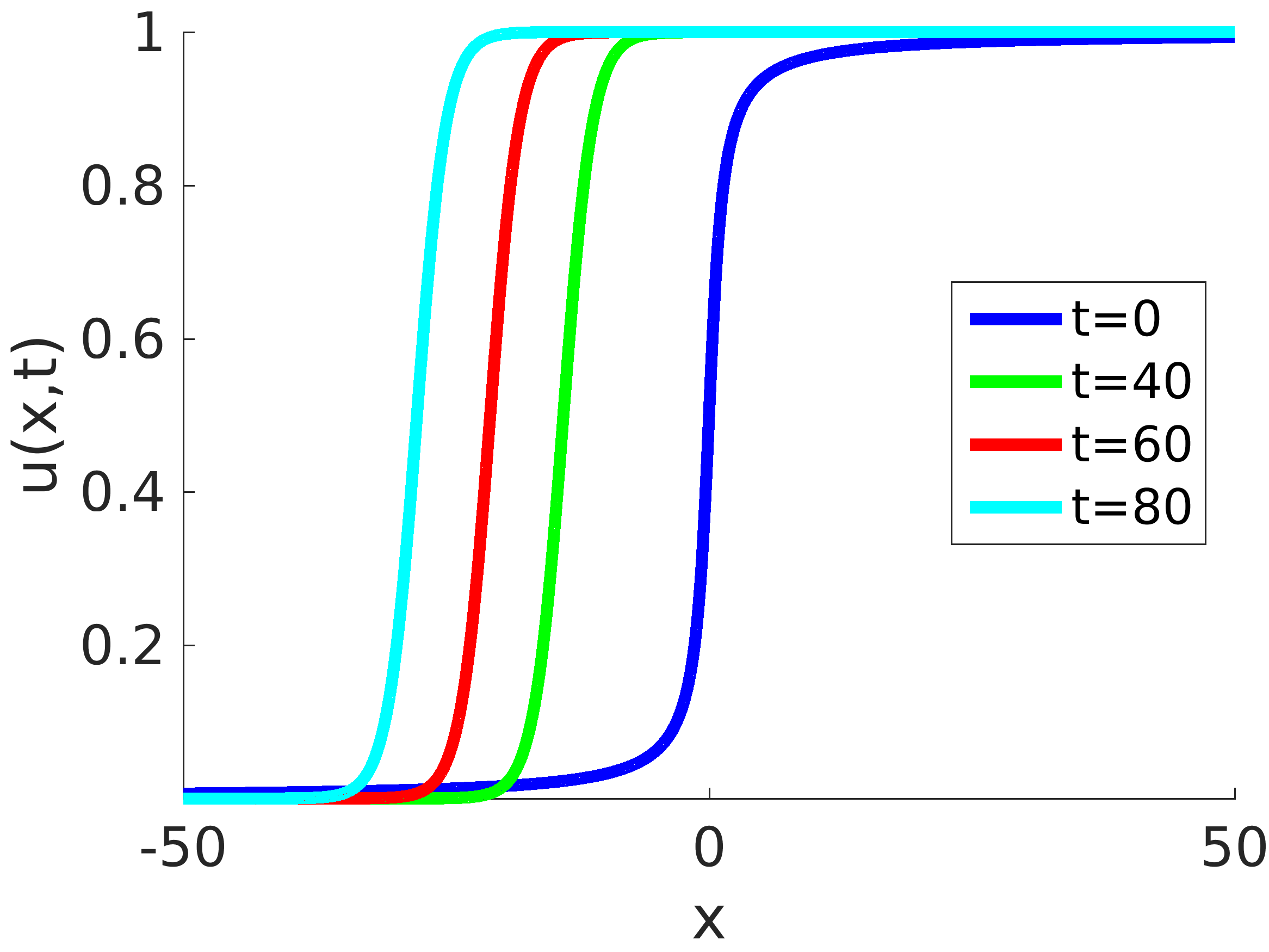
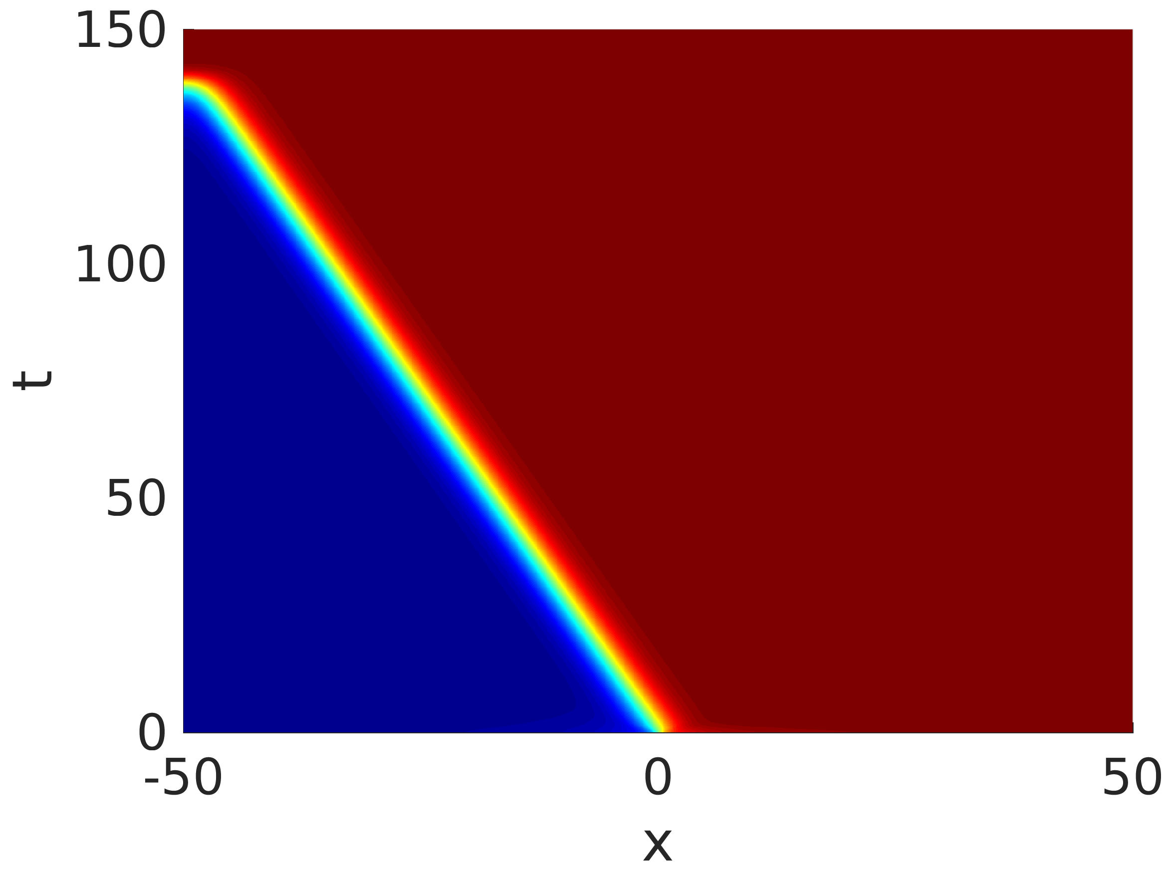
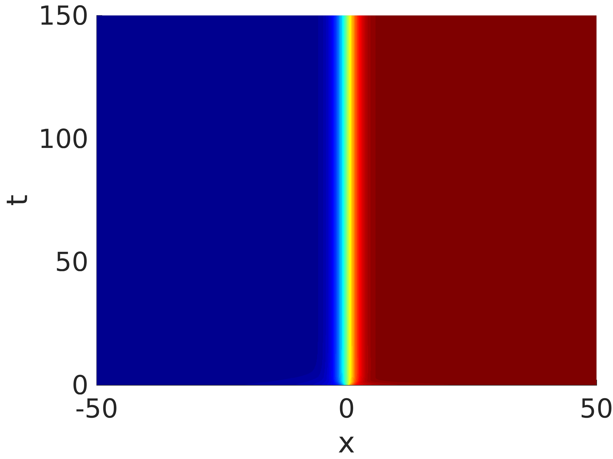
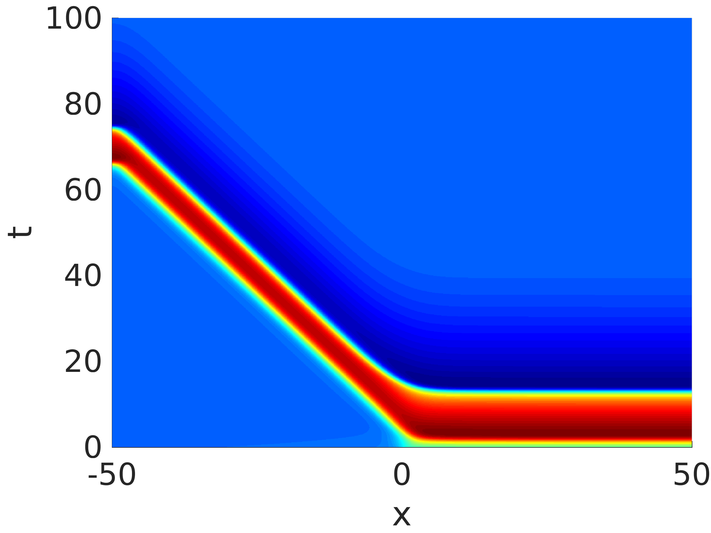
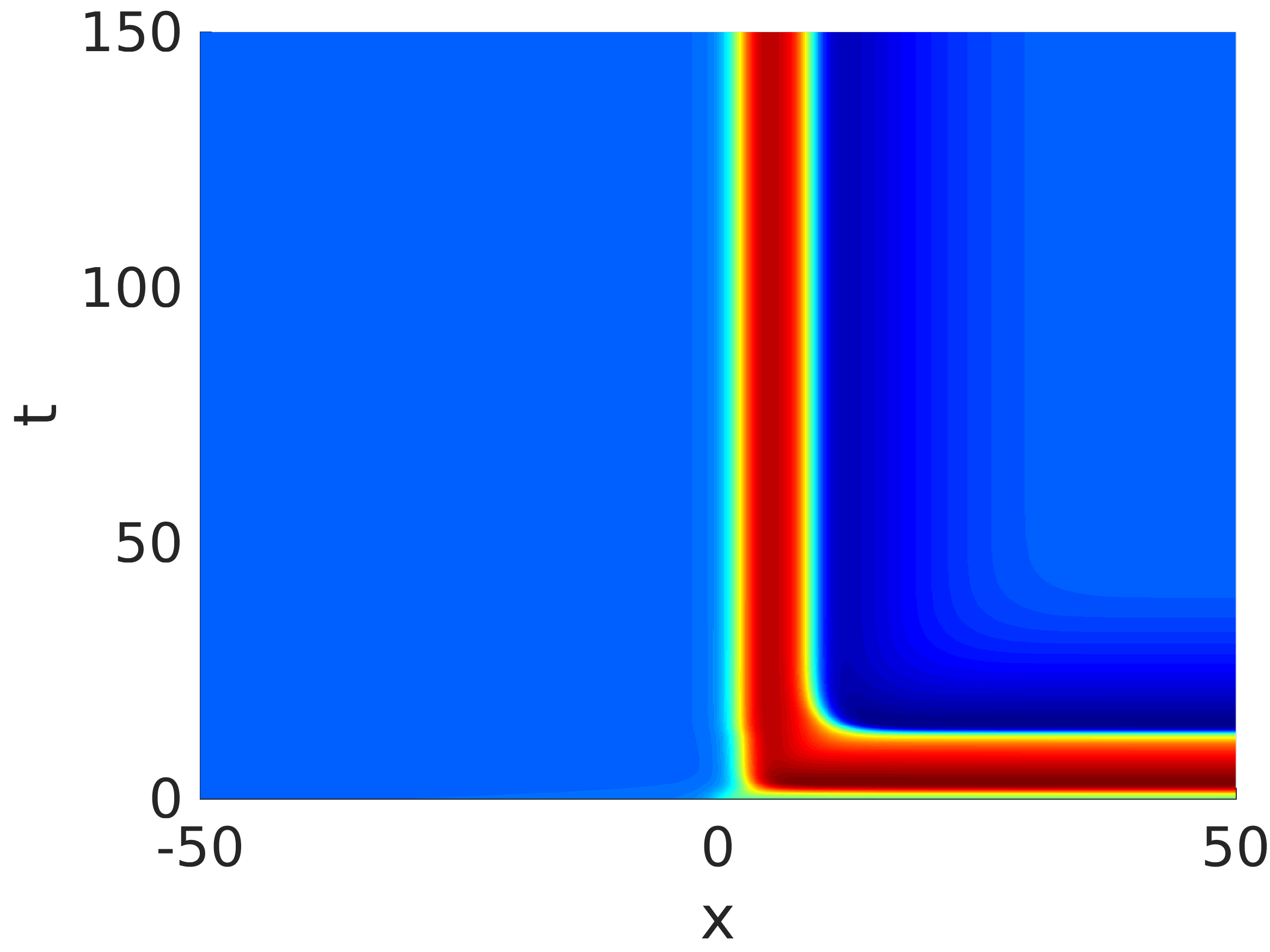
Figure 2.1 shows a numerical approximation of the time evolution of the traveling front solution $u$ of (2.25) on the spatial domain $(-50,50)$ with homogeneous Neumann boundary conditions and initial data

(2.27) $$u_{0}(x)=\frac{1}{\pi}\arctan(x)+\frac{1}{2},\quad v_{0}(x)=0,\quad x\in(-50,50).$$

Further parameter values are $\varepsilon=b=\frac{1}{4}$. For the space discretization we used continuous piecewise linear finite elements with spatial stepsize $\triangle x=0.1$. For the time discretization we used the BDF method of order $2$ with absolute tolerance $\mathrm{atol}=10^{-3}$, relative tolerance $\mathrm{rtol}=10^{-2}$, temporal stepsize $\triangle t=0.1$ and final time $T=150$.

Figure 2.1. Traveling front of Nagumo wave equation (2.25) at different time instances (a) and its time evolution (b) for parameters $\varepsilon=b=\frac{1}{4}$.

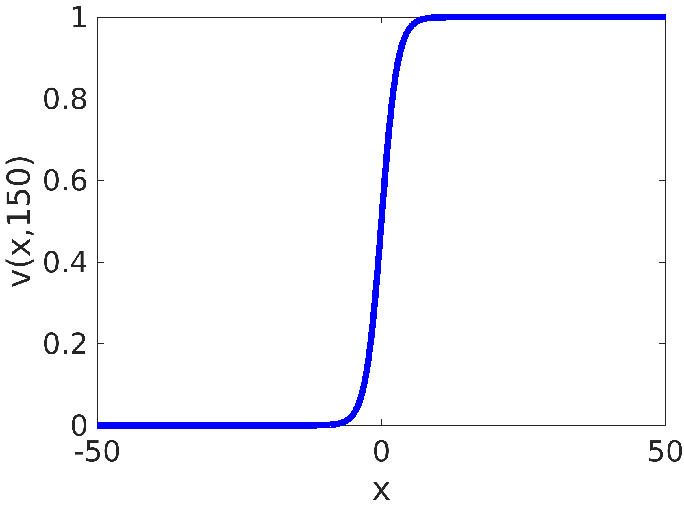
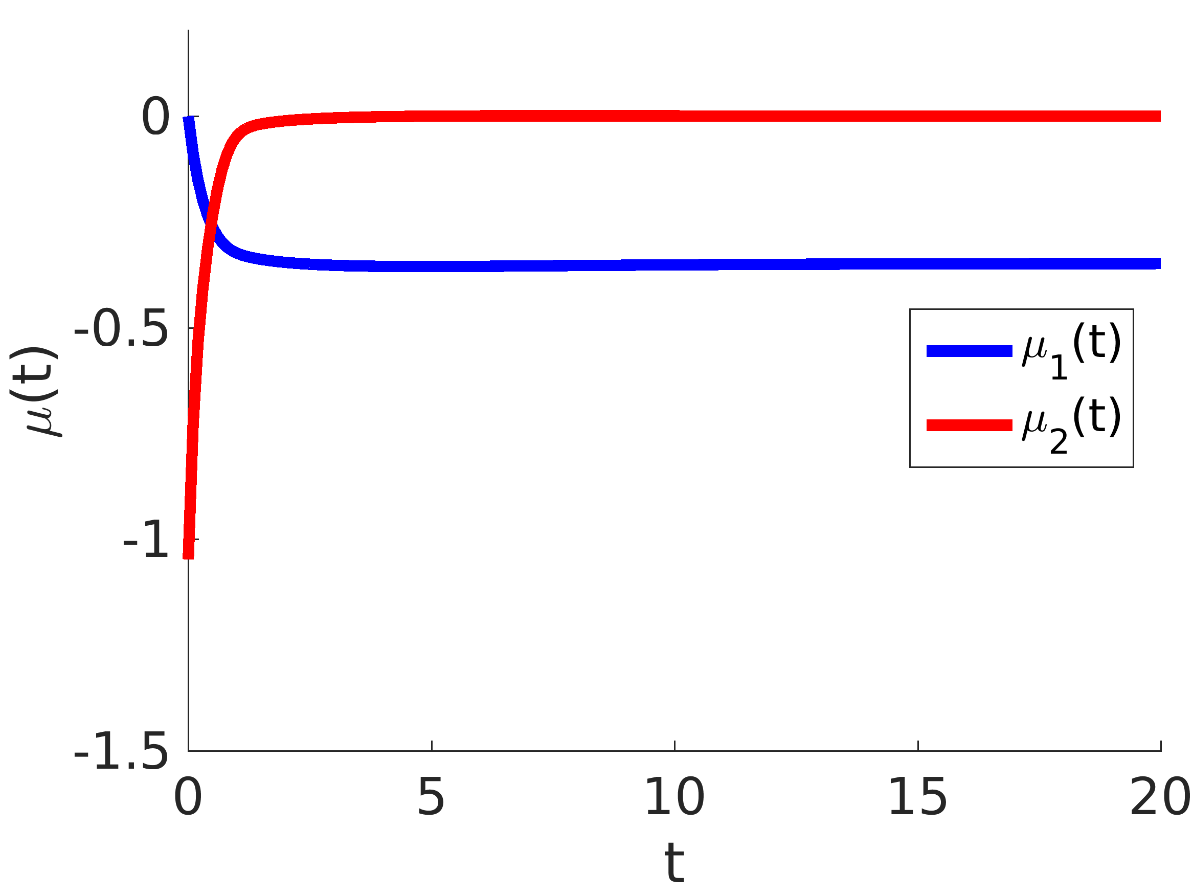
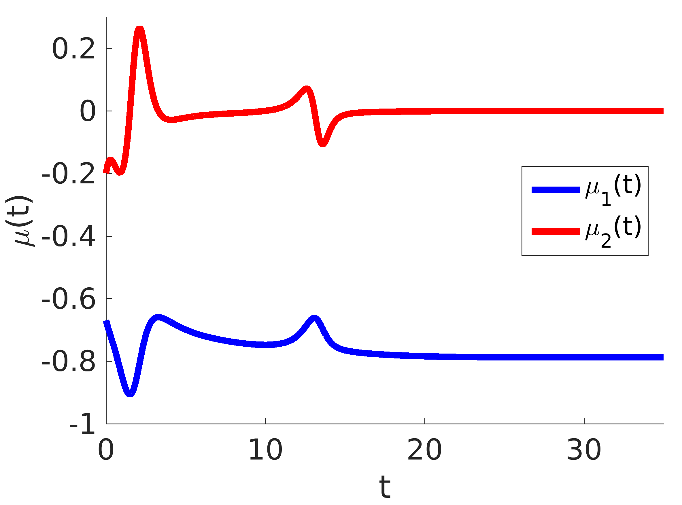
Figure 2.2. Solution of the frozen Nagumo wave equation (2.28): Approximation of profile $v(x,150)$ (a) and time evolutions of velocity $\mu_{1}$ and acceleration $\mu_{2}$ (b) and of the profile $v$ (c) for parameters $\varepsilon=b=\frac{1}{4}$.

Next we solve with the same data the frozen Nagumo wave equation resulting from (2.18)

(2.28a) $$\begin{aligned} \varepsilon v_{tt}+v_{t}&=(1-\mu_{1}^{2}\varepsilon)v_{\xi\xi}+2\mu_{1}\varepsilon v_{\xi,t}+(\mu_{2}\varepsilon+\mu_{1})v_{\xi}+g(v),\\ \mu_{1,t}&=\mu_{2},\quad\gamma_{t}=\mu_{1},\end{aligned} t\geqslant 0,$$

(2.28b) $$0=\bigl{\langle}v_{t}(\cdot,t),\hat{v}_{\xi}\bigr{\rangle}_{L^{2}(\mathbb{R},\mathbb{R})}, t\geqslant 0,$$

(2.28c) $$\begin{aligned} v(\cdot,0)&=u_{0},\quad v_{t}(\cdot,0)=v_{0}+\mu_{1}^{0}u_{0,\xi},\quad\mu_{1}(0)=\mu_{1}^{0},\quad\gamma(0)=0.\end{aligned}$$

Figure 2.2 shows the solution $(v,\mu_{1},\mu_{2},\gamma)$ of (2.28) on the spatial domain $(-50,50)$ with homogeneous Neumann boundary conditions, initial data $u_{0}$, $v_{0}$ from (2.27), and reference function $\hat{v}=u_{0}$. For the computation we used the fixed phase condition $\psi_{\mathrm{fix},2}^{\mathrm{2nd}}(v_{t})$ from (2.10) with consistent intial data $\mu_{1}^{0}$, $\mu_{2}^{0}$, c.f. (2.12) and (2.13). Note that $v_{0}=0$ from (2.27) implies $\mu_{1}^{0}=0$ according to (2.12). Then, inserting $\mu_{1}^{0}=0$, $u_{0},v_{0}$ from (2.27), $\hat{v}=u_{0}$, $M=\varepsilon$, $A=B=1$, $C=0$ and $g$ from (2.24) into (2.13), finally implies $\mu_{2}^{0}=-1.0312$. The discretization data are taken as in the nonfrozen case. The diagrams show that after a very short transition phase the profile becomes stationary, the acceleration $\mu_{2}$ converges to zero, and the speed $\mu_{1}$ approaches an asymptotic value $\mu_{\star}^{\mathrm{num}}$ which is close to the exact value $\mu_{\star}\approx-0.34816$, given by (2.26). We expect $|\mu_{\star}-\mu_{\star}^{\mathrm{num}}|\to 0$ as the domain $(-R,R)$ grows and stepsizes tend to zero.

Note that the unknown function $\gamma(t)$ (not shown), $t\in[0,150]$, is obtained by integrating the last equation in (2.28a). From its values one can still recover the position of the front in the original system (2.25). It turns out that the wave hits the left boundary at $x=-50$ at time $t\approx 143.82$ (cf. Figure 2.1(b)).

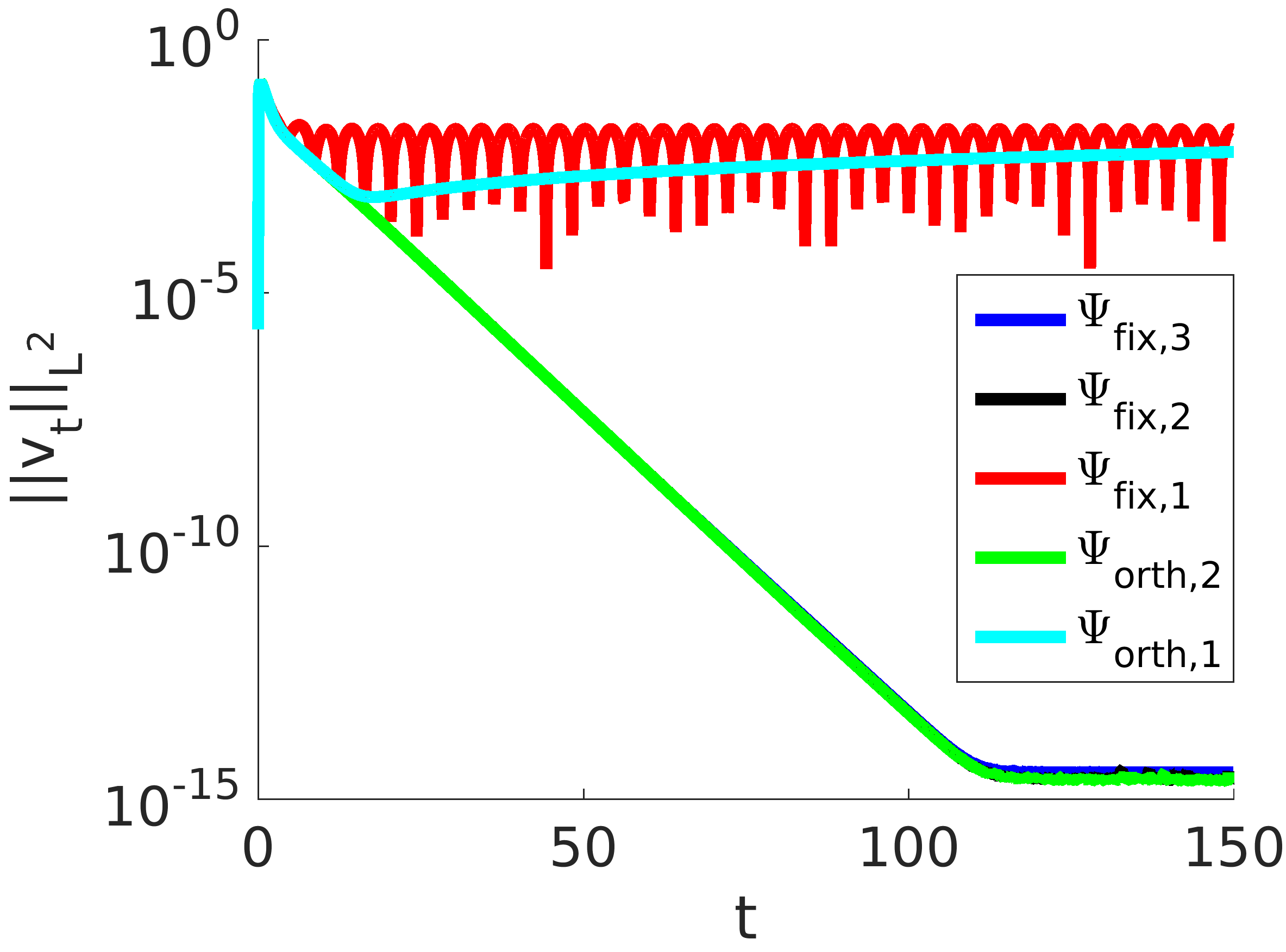
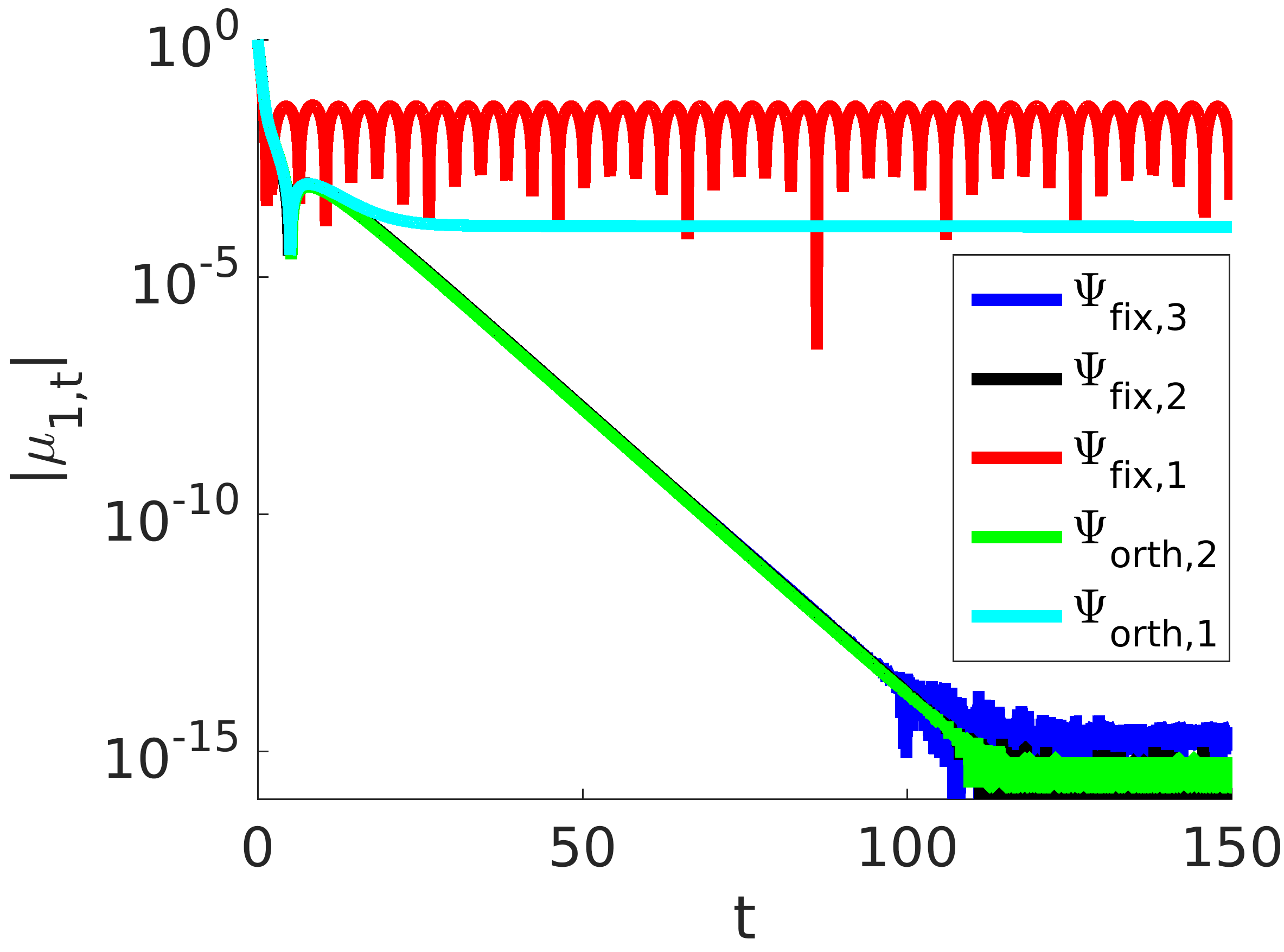
Figure 2.3. Comparison of the phase conditions for the frozen Nagumo wave equation (2.28): Time evolution of $\left\|v_{t}\right\|_{L^{2}}$ (a) and $|\mu_{1,t}|$ (b) for parameters $\varepsilon=b=\frac{1}{4}$.

If we replace the phase condition $\psi_{\mathrm{fix},2}^{\mathrm{2nd}}$ in (2.28) by $\psi_{\mathrm{fix},3}^{\mathrm{2nd}}$ or $\psi_{\mathrm{orth},2}^{\mathrm{2nd}}$, we obtain very similar results as those from Figure 2.2. The profile again becomes stationary, the acceleration $\mu_{2}$ converges to zero, and the speed $\mu_{1}$ approaches to an asymptotic value. Since we expect $v_{t}(t)\to 0$ and $\mu_{1,t}(t)\to 0$ as $t\to\infty$, we use these quantities as an indicator checking whether the solution has become stationary. Figure 2.3 shows the time evolution of $\left\|v_{t}\right\|_{L^{2}}$ and $|\mu_{1,t}|$ when solving (2.28) for different phase conditions. While the phase conditions of index $2$ and $3$ behave as expected, the index $1$ formulation yields small but oscillating values for the norms of $v_{t}$ and $\mu_{1,t}$. We attribute this behavior to the fact, that our adaptive solver enforces the differentiated conditions (2.11), (2.15), but does not control $v_{t},\mu_{t}$ directly. Further investigations show that the consistency condition for $\mu_{2}^{0}$ does not really affect the numerical results for the different phase conditions. Therefore, in the next example we do not compute the expression for $\mu_{2}^{0}$ but use the expected limiting value as initial datum $\mu_{2}^{0}=0$.

Example 2.4 (FitzHugh-Nagumo wave system).

Consider the $2$-dimensional parabolic FitzHugh-Nagumo system, [10],

(2.29) $$u_{t}=\tilde{A}u_{xx}+g(u),\;x\in\mathbb{R},\,t\geq 0,\quad\tilde{A}=\begin{pmatrix}1&0\\ 0&\rho\end{pmatrix},\;g(u)=\begin{pmatrix}u_{1}-\frac{1}{3}u_{1}^{3}-u_{2}\\ \phi(u_{1}+a-bu_{2})\end{pmatrix},$$

with $u=u(x,t)\in\mathbb{R}^{2}$ and positive parameters $\rho,a,b,\phi\in\mathbb{R}$. Equation (2.29) is known to exhibit traveling wave solutions in a wide range of parameters, but there are apparently no explicit formulas. For the values

(2.30) $$\rho=0.1,\quad a=0.7,\quad\phi=0.08,\quad b=0.8$$

one finds a traveling pulse with

(2.31) $$w_{\pm}\approx(-1.19941,\,-0.62426)^{\top},\quad c_{\star}\approx-0.7892.$$

For the same $\rho,a,\phi$ but $b=3$, there is a traveling front with asymptotic states and velocity given by

$$w_{-}\approx(1.18779,\,0.62923)^{\top},\quad w_{+}\approx(-1.56443,\,-0.28814)^{\top},\quad c_{\star}\approx-0.8557.$$

Applying Proposition 2.1(i) with $M=\varepsilon I_{2}$ requires the equality $\tilde{A}+c_{\star}^{2}M=k^{2}A$, i.e.

$$1+c_{\star}^{2}\varepsilon=k^{2}A_{11},\quad\rho+c_{\star}^{2}\varepsilon=k^{2}A_{22},\quad A_{12}=A_{21}=0.$$

Setting $A_{11}:=1$ und using parameter values from (2.30), Proposition 2.1(i) shows that the corresponding FitzHugh-Nagumo wave system

(2.32) $$Mu_{tt}+Bu_{t}=Au_{xx}+g(u),\;x\in\mathbb{R},\,t\geq 0,$$

with

$$M=\varepsilon I_{2},\quad B=I_{2},\quad A=\mathrm{diag}(1,\tfrac{\rho+c_{\star}^{2}\varepsilon}{1+c_{\star}^{2}\varepsilon}),\quad k=\sqrt{1+c_{\star}^{2}\varepsilon},\quad\varepsilon>0,\quad\rho,c_{\star}\text{ given}$$

has a traveling pulse (or a traveling front) solution with a scaled profile $v_{\star}$, limits $v_{\pm}=w_{\pm}$, and velocity $\mu_{\star}=\frac{c_{\star}}{k}$.

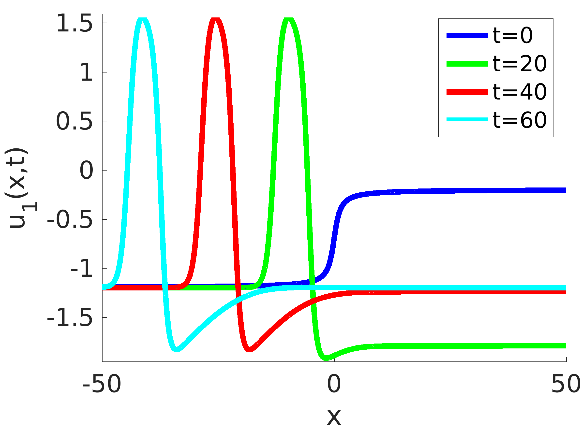
In the following we show the computations for the traveling pulse. Results for the traveling front are very similar and are not displayed here. In the frozen and the nonfrozen case, we choose $\varepsilon=10^{-2}$ and parameter value (2.30). Space and time are discretized as in Example 2.3. Figure 2.4 shows the time evolution of the traveling pulse solution $u=(u_{1},u_{2})^{T}$ of (2.32) on the spatial domain $(-50,50)$ with homogeneous Neumann boundary conditions. The initial data are

(2.33) $$u_{0}(x)=(\tfrac{1}{\pi}\arctan(x)+\tfrac{1}{2},\,0)^{\top}+v_{\pm},\quad v_{0}(x)=(0,\,0)^{\top},\quad x\in\mathbb{R},$$

where $v_{\pm}=w_{\pm}$ is the asymptotic state from (2.31).

Figure 2.4. Traveling pulse of FitzHugh-Nagumo wave system (2.32) at different time instances for $u_{1}$ (a) as well as its time evolutions (c) for parameters $\varepsilon=10^{-2}$, $\rho=0.1$, $a=0.7$, $\phi=0.08$ and $b=0.8$.

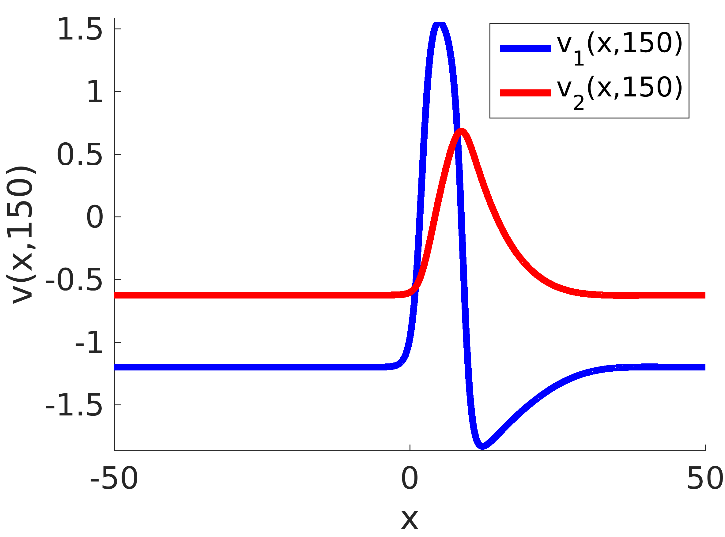
Figure 2.5. Solution of the frozen FitzHugh-Nagumo wave system (2.18): Approximation of profile components $v_{1}(x,150)$, $v_{2}(x,150)$ (a), and time evolutions of velocity $\mu_{1}$ and acceleration $\mu_{2}$ (b) and of the profile’s component $v_{1}$ (c) for parameters $\varepsilon=10^{-2}$, $\rho=0.1$, $a=0.7$, $\phi=0.08$ and $b=0.8$.

Next consider for the same parameter values the corresponding frozen FitzHugh-Nagumo wave system

(2.34a) $$\begin{aligned} Mv_{tt}+Bv_{t}&=(A-\mu_{1}^{2}M)v_{\xi\xi}+2\mu_{1}Mv_{\xi,t}+(\mu_{2}M+\mu_{1}B)v_{\xi}+g(v),\\ \mu_{1,t}&=\mu_{2},\quad\gamma_{t}=\mu_{1},\end{aligned} t\geqslant 0,$$

(2.34b) $$0=\bigl{\langle}v_{t}(\cdot,t),\hat{v}_{\xi}\bigr{\rangle}_{L^{2}(\mathbb{R},\mathbb{R})}, t\geqslant 0,$$

(2.34c) $$\begin{aligned} v(\cdot,0)&=u_{0},\quad v_{t}(\cdot,0)=v_{0}+\mu_{1}^{0}u_{0,\xi},\quad\mu_{1}(0)=\mu_{1}^{0},\quad\gamma(0)=0.\end{aligned}$$

Figure 2.5 shows the solution $(v,\mu_{1},\mu_{2},\gamma)$ of (2.34) on the spatial domain $(-50,50)$, with homogeneous Neumann boundary conditions, initial data $u_{0}$, $v_{0}$ from (2.33), and reference function $\hat{v}=u_{0}$. For the computation we used again the fixed phase condition $\psi_{\mathrm{fix},2}^{\mathrm{2nd}}(v_{t})$ from (2.10) with consistent intial data for $\mu_{1}^{0}$. Note that $v_{0}=0$ from (2.33) implies $\mu_{1}^{0}=0$ according to (2.12). We further set $\mu_{2}^{0}=0$ which does not satisfy the consistency condition (2.13). Time and space discretization are done as in the nonfrozen case. Again the profile quickly stabilizes and the velocity and the acceleration reach their asymptotic values.

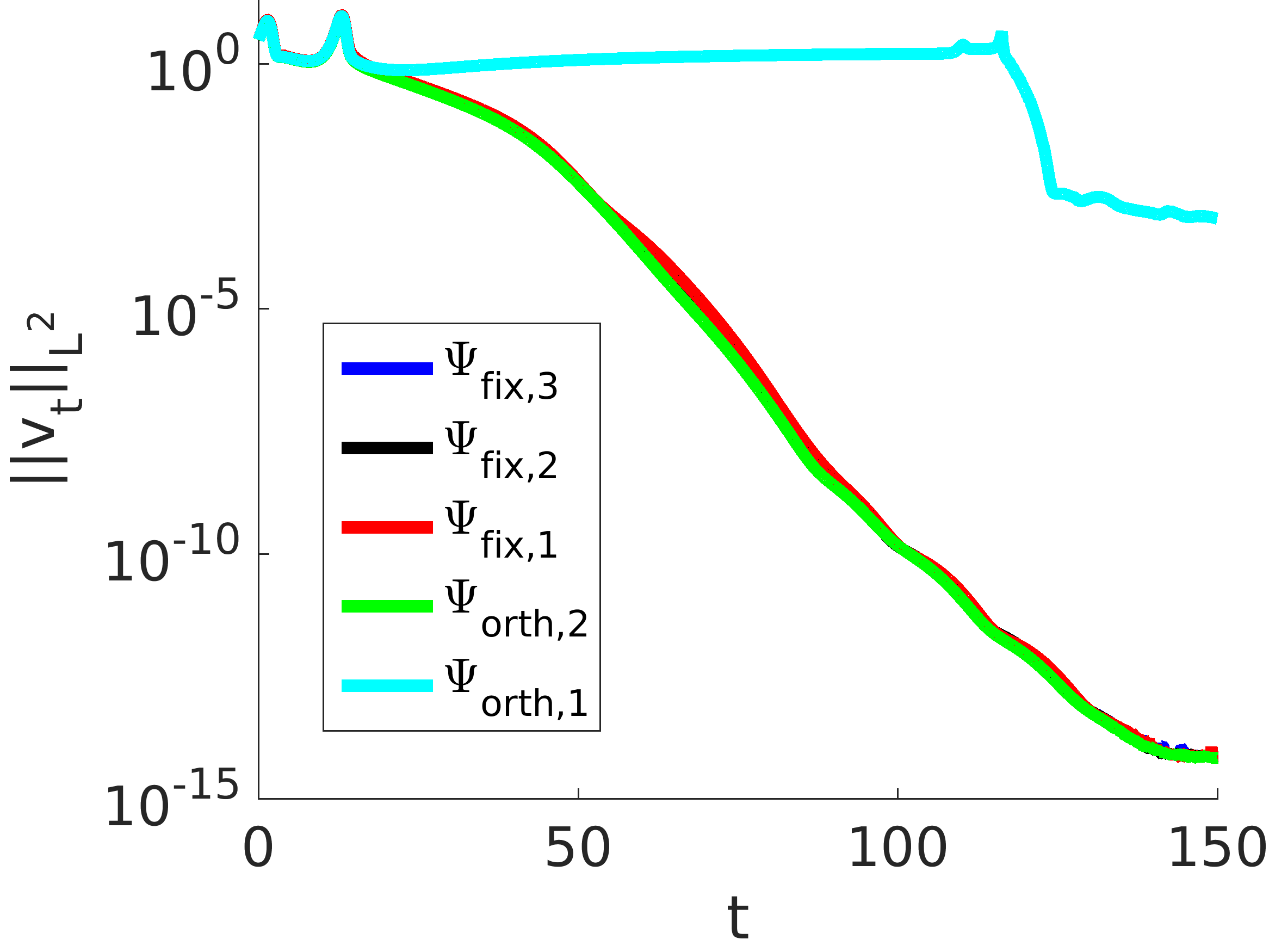
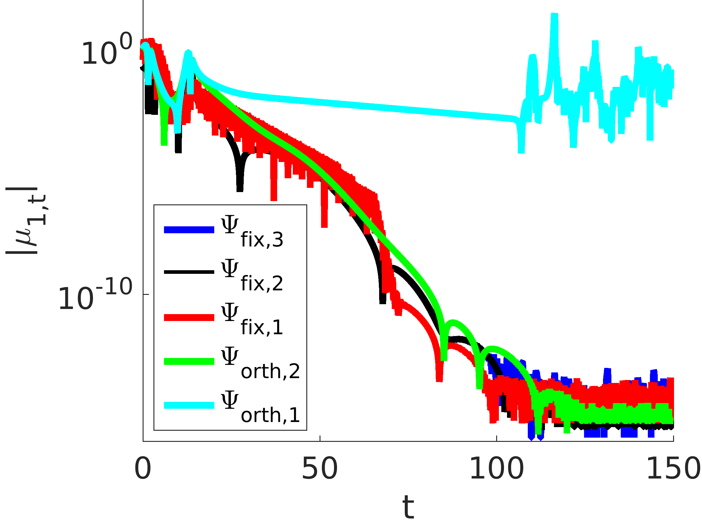
Figure 2.6. Comparison of the phase conditions for the frozen FitzHugh-Nagumo wave system (2.34): Time evolution of $\left\|v_{t}\right\|_{L^{2}}$ (a) and $|\mu_{1,t}|$ (b) for parameters $\varepsilon=10^{-2}$, $\rho=0.1$, $a=0.7$, $\phi=0.08$ and $b=0.8$.

Finally, Figure 2.6 shows that similar results are obtained if we replace the phase condition $\psi_{\mathrm{fix},2}^{\mathrm{2nd}}$ in the frozen FitzHugh-Nagumo wave system (2.34) by $\psi_{\mathrm{fix},3}^{\mathrm{2nd}}$, $\psi_{\mathrm{fix},1}^{\mathrm{2nd}}$, $\psi_{\mathrm{orth},2}^{\mathrm{2nd}}$, or even by $\psi_{\mathrm{orth},1}^{\mathrm{2nd}}$. Contrary to our first example, the fixed phase condition of index $1$ provides good results in this case, while the index $1$ formulation of the orthogonal phase condition $\psi_{\mathrm{orth},1}^{\mathrm{2nd}}$ continues to show small oscillations of the time derivatives.

3. Spectra and eigenfunctions of traveling waves

In this section we study the spectrum of the quadratic operator polynomial (cf. (1.8))

(3.1) $$\mathcal{P}(\lambda):=\lambda^{2}P_{2}+\lambda P_{1}+P_{0},\quad\lambda\in\mathbb{C}.$$

Here the differential operators $P_{j}$ are defined by

(3.2) $$P_{2}=M,\;\;P_{1}=-D_{3}f(\star)-2\mu_{\star}M\partial_{\xi},\;\;P_{0}=-(A-\mu_{\star}^{2}M)\partial_{\xi}^{2}+(\mu_{\star}D_{3}f(\star)-D_{2}f(\star))\partial_{\xi}-D_{1}f(\star),$$

where $(\star)=(v_{\star},v_{\star,\xi},-\mu_{\star}v_{\star,\xi})$ and $v_{\star}$, $\mu_{\star}$ denote the profile and velocity of a traveling wave solution $u_{\star}(x,t)=v_{\star}(x-\mu_{\star}t)$ of (1.1). Note that $P_{j}$ is a differential operator of order $2-j$ for $j=0,1,2$. In the following we recall some standard notions of point and essential spectrum for operator polynomials.

Definition 3.1.

Let $(X,\left\|\cdot\right\|_{X})$ and $(Y,\left\|\cdot\right\|_{Y})$ be complex Banach spaces and let $\mathcal{P}(\lambda)=\sum_{j=0}^{q}P_{j}\lambda^{j},\lambda\in\mathbb{C}$ be an operator polynomial with linear continuous coefficients $P_{j}:Y\rightarrow X$, $j=0,\ldots,q$.

• The resolvent set $\rho(\mathcal{P})$ and the spectrum $\sigma(\mathcal{P})$ are defined by

  $$\rho(\mathcal{P})=\{\lambda\in\mathbb{C}:\mathcal{P}(\lambda)\;\text{is bijective and}\quad\mathcal{P}(\lambda)^{-1}:X\rightarrow Y\;\text{is bounded}\},\;\sigma(\mathcal{P}):=\mathbb{C}\backslash\rho(\mathcal{P}).$$

• $\lambda_{0}\in\sigma(\mathcal{P})$ is called isolated if there is $\varepsilon>0$ such that $\lambda\in\rho(\mathcal{P})$ for all $\lambda_{0}\neq\lambda\in\mathbb{C}$ with $|\lambda-\lambda_{0}|<\varepsilon$.

• If $\mathcal{P}(\lambda_{0})y_{0}=0$ for some $\lambda_{0}\in C$ and $y_{0}\in Y\setminus\{0\}$, then $\lambda_{0}$ is called an eigenvalue with eigenvector $y_{0}$. The eigenvalue $\lambda_{0}$ has finite multiplicity if $\dim(\mathcal{N}(\mathcal{P}(\lambda_{0})))<\infty$ and if there is a maximum number $n\in\mathbb{N}$, for which polynomials $y(\lambda)=\sum_{j=0}^{r}(\lambda-\lambda_{0})^{j}y_{j}$ exist in $Y$ satisfying

  (3.3) $$y_{0}\neq 0,\quad(\mathcal{P}y)^{(\nu)}(\lambda_{0})=0,\quad\nu=0,\ldots,n-1.$$

  This maximum number $n=n(\lambda_{0})$ is called the maximum partial multiplicity, and $\dim(\mathcal{N}(\mathcal{P}(\lambda_{0})))$ is called the geometric multiplicity of $\lambda_{0}$.

• The point spectrum is defined by

  $$\sigma_{\mathrm{point}}(\mathcal{P})=\{\lambda\in\sigma(\mathcal{P}):\;\text{$\lambda$ is isolated eigenvalue of finite multiplicity}\}.$$

  Points in $\rho(\mathcal{P})\cup\sigma_{\mathrm{point}}(\mathcal{P})$ are called normal, and the essential spectrum of $\mathcal{P}$ is defined by

  $$\sigma_{\mathrm{ess}}(\mathcal{P}):=\{\lambda\in\mathbb{C}:\;\text{$\lambda$ is not a normal point of $\mathcal{P}$}\}.$$

Remark 3.2.

There is no loss of generality in assuming the root polynomials in (c) to be of the form $y(\lambda)=\sum_{j=0}^{n-1}(\lambda-\lambda_{0})^{j}y_{j}$. For if $r<n-1$ we simply set $y_{j}=0,j=r+1,\ldots,n-1$. And if $r\geq n$ we subtract from $y$ the term $\sum_{j=n}^{r}(\lambda-\lambda_{0})^{j}y_{j}$ which has $\lambda_{0}$ as a zero of order at least $n$ and thus does not change the root property (3.3). The eigenvalue $\lambda_{0}$ is simple iff the geometric and the maximum partial multiplicity are equal to $1$. In this case $\mathcal{N}(\mathcal{P}(\lambda_{0}))=\mathrm{span}(y_{0})$ for some $y_{0}\neq 0$ and $\mathcal{P}^{\prime}(\lambda_{0})y_{0}\notin\mathcal{R}(\mathcal{P}(\lambda_{0}))$. For more details on root polynomials, partial and algebraic multiplicities we refer to [20, 21, 22]. Our definition of essential spectrum follows [18].

By definition, the spectrum $\sigma(\mathcal{P})$ of $\mathcal{P}$ can be decomposed into its point spectrum and its essential spectrum

$$\sigma(\mathcal{P})=\sigma_{\mathrm{ess}}(\mathcal{P})\,\dot{\cup}\,\sigma_{\mathrm{point}}(\mathcal{P}).$$

The function spaces underlying the definition of spectra are subspaces of $L^{2}(\mathbb{R},\mathbb{R}^{m})$ which will be specified in Section 4 and Appendix A. In this section we carry out formal calculations without reference to a specific function space.

3.1. Point spectrum on the imaginary axis

Applying $\partial_{\xi}$ to the traveling wave equation (1.6), leads to the equation

$$\begin{split}0=&(A-\mu_{\star}^{2}M)v_{\star,\xi\xi\xi}+D_{2}f(\star)v_{\star,\xi\xi}+D_{1}f(\star)v_{\star,\xi}-\mu_{\star}D_{3}f(\star)v_{\star,\xi\xi}=-P_{0}v_{\star,\xi},\,\xi\in\mathbb{R},\end{split}$$

provided that $v_{\star}\in C^{3}(\mathbb{R},\mathbb{R}^{m})$ and $f\in C^{1}(\mathbb{R}^{3m},\mathbb{R}^{m})$. Therefore, $w=v_{\star,\xi}$ solves the quadratic eigenvalue problem $\mathcal{P}(\lambda)w=0$ for $\lambda=0$, and $w=v_{\star,\xi}$ is an eigenfunction if the wave profile $v_{\star}$ is nontrivial (i.e. not constant). This behavior is to be expected since the original equation is equivariant with respect to the shift, and the spatial derivative $\partial_{\xi}$ is the generator of shift equivariance.

Proposition 3.3 (Point spectrum of traveling waves).

Let $v_{\star}\in C^{3}(\mathbb{R},\mathbb{R}^{m})$, $\mu_{\star}$ be a nontrivial classical solution of (1.6) and $f\in C^{1}(\mathbb{R}^{3m},\mathbb{R}^{m})$. Then $\lambda=0$ is an eigenvalue with eigenfunction $v_{\star,\xi}$ of the quadratic eigenvalue problem $\mathcal{P}(\lambda)w=0$. In particular, $0\in\sigma_{\mathrm{point}}(\mathcal{P})$.

As usual, further isolated eigenvalues are difficult to detect analytically, and we refer to the extensive literature on solving quadratic eigenvalue problems and on locating zeros of the so-called Evans function, see e.g. [2, 32].

Example 3.4 (Nagumo wave equation).

Recall from Example 2.3 that the Nagumo wave equation (2.25) has an explicit traveling front solution $u_{\star}(x,t)=v_{\star}(\xi)$, $\xi=x-\mu_{\star}t$, with $v_{\star}$ and $\mu_{\star}$ from (2.26), i.e. $v_{\star}$ and $\mu_{\star}$ solve the associated traveling wave equation

$$0=(1-\mu_{\star}^{2}\varepsilon)v_{\star,\xi\xi}(\xi)+\mu_{\star}v_{\star,\xi}(\xi)+v_{\star}(\xi)\left(1-v_{\star}(\xi)\right)\left(v_{\star}(\xi)-b\right),\quad\xi\in\mathbb{R}.$$

The quadratic eigenvalue problem for the linearization then reads as follows,

$$[\mathcal{P}(\lambda)w](\xi)=\varepsilon\left(\lambda-\mu_{\star}\partial_{\xi}\right)^{2}w(\xi)+\left(\lambda-\mu_{\star}\partial_{\xi}\right)w(\xi)-w_{\xi\xi}(\xi)+\left(3v_{\star}^{2}(\xi)-2(b+1)v_{\star}(\xi)-b\right)w(\xi)=0,\;\xi\in\mathbb{R}.$$

With $k$ from (2.26), it has the solution

$$\lambda=0,\quad w(\xi)=v_{\star,\xi}(\xi)=\tfrac{k}{\sqrt{2}}\exp\left(-\tfrac{k\xi}{\sqrt{2}}\right)\left(1+\exp\left(-\tfrac{k\xi}{\sqrt{2}}\right)\right)^{-2},\quad\xi\in\mathbb{R}.$$

3.2. Essential spectrum and dispersion relation of traveling waves

The essential spectrum of $\mathcal{P}$ from (3.1), (3.2), is determined by the constant coefficient operators obtained by letting $\xi\rightarrow\pm\infty$ in the coefficient operators $P_{0},P_{1}$ (recall $(\pm)=(v_{\pm},0,0)$),

(3.4) $$\mathcal{P}^{\pm}(\lambda)= \lambda^{2}P_{2}+\lambda P_{1}^{\pm}+P_{0}^{\pm},\quad\lambda\in\mathbb{C},$$

$$P_{1}^{\pm}= -D_{3}f(\pm)-2\mu_{\star}M\partial_{\xi},\quad P_{0}^{\pm}=-(A-\mu_{\star}^{2}M)\partial_{\xi}^{2}+(\mu_{\star}D_{3}f(\pm)-D_{2}f(\pm))\partial_{\xi}-D_{1}f(\pm).$$

We seek bounded solutions $w$ of $\mathcal{P}^{\pm}(\lambda)w=0$ by the Fourier ansatz $w(\xi)=e^{i\omega\xi}z,z\in\mathbb{C}^{m},|z|=1$ and arrive at the following quadratic eigenvalue problem

$$\mathcal{A}_{\pm}(\lambda,\omega)z=\left(\lambda^{2}A_{2}+\lambda A_{1}^{\pm}(\omega)+A_{0}^{\pm}(\omega)\right)z=0$$

with matrices

(3.5) $$A_{2}=M,\quad A_{1}^{\pm}(\omega)=-D_{3}f(\pm)-2i\omega\mu_{\star}M,\quad A_{0}^{\pm}(\omega)=\omega^{2}(A-\mu_{\star}^{2}M)+i\omega(\mu_{\star}D_{3}f(\pm)-D_{2}f(\pm))-D_{1}f(\pm).$$

Every $\lambda\in\mathbb{C}$ satisfying the dispersion relation

(3.6) $$\det\left(\lambda^{2}A_{2}+\lambda A_{1}^{\pm}(\omega)+A_{0}^{\pm}(\omega)\right)=0$$

for some $\omega\in\mathbb{R}$ and either sign, belongs to the essential spectrum of $\mathcal{P}$. A proof of this statement is obtained in the standard way by cutting off $w(\xi)$ at $\xi\notin[n,2n]$ resp. $\xi\notin[-2n,-n]$ and letting $n\rightarrow\infty$. Then this contradicts the continuity of the resolvent at $\lambda$ in appropriate function spaces. This proves the following result:

Proposition 3.5 (Essential spectrum of traveling waves).

Let $f\in C^{1}(\mathbb{R}^{3m},\mathbb{R}^{m})$ with $f(v_{\pm},0,0)=0$ for some $v_{\pm}\in\mathbb{R}^{m}$. Let $v_{\star}\in C^{2}(\mathbb{R},\mathbb{R}^{m})$, $\mu_{\star}$ be a nontrivial classical solution of (1.6) satisfying $v_{\star}(\xi)\to v_{\pm}$ as $\xi\to\pm\infty$. Then, the dispersion set set

(3.7) $$\sigma_{\mathrm{disp}}(\mathcal{P}):=\left\{\lambda\in\mathbb{C}\mid\text{$\lambda$ satisfies \eqref{equ:4.12} for some $\omega\in\mathbb{R}$ and some sign $\pm$}\right\}$$

belongs to the essential spectrum $\sigma_{\mathrm{ess}}(\mathcal{P})$ of $\mathcal{P}$.

In the general matrix case it is not easy to analyze the shape of the algebraic set $\sigma_{\mathrm{disp}}(\mathcal{P})$, since (3.6) amounts to finding the zeroes of a polynomial of degree $2m$. In view of the stability results in Theorem 4.8 and Theorem 4.10 our main interest is in finding a spectral gap, i.e. a constant $\beta>0$ such that

(3.8) $$\mathrm{Re}\,\lambda\leq-\beta<0\quad\text{for all}\quad\lambda\in\sigma_{\mathrm{disp}}(\mathcal{P}).$$

We discuss this condition for three subcases of the special structure (1.2).

• Parabolic case: ($\mathbf{M=0}$, $\mathbf{B=I_{m}}$, $\mathbf{C=0}$). The dispersion relation (3.6) reads

  (3.9) $$\det\left(\tilde{\lambda}I_{m}+\omega^{2}A-Dg(v_{\pm})\right)=0,\quad\tilde{\lambda}=\lambda-i\omega\mu_{\star},$$

  and the corresponding eigenvalue problem may be written as

  (3.10) $$\tilde{\lambda}z=-\left(\omega^{2}A-Dg(v_{\pm})\right)z,\quad 0\neq z\in\mathbb{C}^{m},\quad\tilde{\lambda}=\lambda-i\omega\mu_{\star}.$$

  Let us assume positivity of $A$ and $-Dg(v_{\pm})$ in the sense that

  (3.11) $$\mathrm{Re}\,z^{H}Az>0,\quad\mathrm{Re}\,z^{H}Dg(v_{\pm})z<0\quad\text{for all}\;z\in\mathbb{C}^{m}.$$

  Multiplying (3.10) by $z^{H}$ and taking the real part, shows that the solutions $\tilde{\lambda}$ of (3.9) have negative real parts and the gap is guaranteed. This is still true if $A$ is nonnegative but has zero eigenvalues. Note that in this case, equation (2.1) is of mixed hyperbolic-parabolic type and the nonlinear stability theory becomes considerably more involved, see [29].

• Undamped hyperbolic case: ($\mathbf{M=I_{m}}$, $\mathbf{B=0}$, $\mathbf{C=0}$). The dispersion relation (3.6) reads

  $$\det\left(\tilde{\lambda}^{2}I_{m}+\omega^{2}A-Dg(v_{\pm})\right)=0,\quad\tilde{\lambda}=\lambda-i\omega\mu_{\star}$$

  Whenever $\lambda\in\mathbb{C},\omega\in\mathbb{R}$ solve this system, so does the pair $-\lambda,-\omega$. Hence, the eigenvalues lie either on the imaginary axis or on both sides of the imaginary axis. Therefore, a spectral gap cannot exist. This is the Hamiltonian case, where one can only expect stability (but not asymptotic stability) of the wave. We refer to the local stability theory developed in [14],[15] (see also [19] for a recent account). Note that in this case the positivity assumption (3.11) only guarantees $\mathrm{Re}\,\tilde{\lambda}^{2}<0$, i.e. $\tfrac{\pi}{4}<|\mathrm{arg}(\tilde{\lambda})|\leqslant\tfrac{\pi}{2}$ for $\tilde{\lambda}=\lambda-i\omega\mu_{\star}$ and all eigenvalues $\lambda\in\sigma(\mathcal{A}(\cdot,\omega))$.

• Scalar case: ($\mathbf{M=1}$, $\mathbf{B=\eta}$, $\mathbf{C=0}$). It is instructive to discuss the dispersion relation (3.6) in the scalar case with $A=a$, $-Dg(v_{\pm})=\delta$ and real numbers $a,\eta,\delta>0$

  (3.12) $$\tilde{\lambda}^{2}+\eta\tilde{\lambda}+a\omega^{2}+\delta=0,\quad\tilde{\lambda}=\lambda-i\omega\mu_{\star}.$$

  This case occurs with the Nagumo wave equation below. The solutions are

  $$\lambda=i\omega\mu_{\star}-\frac{\eta}{2}\pm\left(\frac{\eta^{2}}{4}-\delta-\omega^{2}a\right)^{1/2},\quad\omega\in\mathbb{R}.$$

  If $\eta^{2}\leq 4\delta$, then all solutions $\lambda$ of (3.12) lie on the vertical line $\mathrm{Re}\,\lambda=-\frac{\eta}{2}<0$. A short discussion shows that they actually cover this line under the assumption $\mu_{\star}^{2}<a$, which corresponds to positivity of the matrix $A-\mu_{\star}^{2}M$ occuring in (1.6). If $\eta^{2}>4\delta$ then the solutions $\lambda$ of (3.12) lie again on this line (resp. cover it if $\mu_{\star}^{2}<a$) for values $|\omega|\geq\omega_{0}:=(\frac{1}{a}(\frac{\eta^{2}}{4}-\delta))^{1/2}$. But for values $|\omega|\leq\omega_{0}$ they form the ellipse

  (3.13) $$\frac{(\mathrm{Re}\,\lambda+\frac{\eta}{2})^{2}}{p_{1}^{2}}+\frac{(\mathrm{Im}\,\lambda)^{2}}{p_{2}^{2}}=1,\quad\text{with semiaxes}\quad p_{1}=a^{1/2}\omega_{0},\;\;p_{2}=|\mu_{\star}|\omega_{0}.$$

  The rightmost point of the ellipse $-\beta:=-\frac{\eta}{2}+\left(\frac{\eta^{2}}{4}-\delta\right)^{1/2}$ is still negative and therefore can be taken for the spectral gap (3.8).

Example 3.6 (Spectrum of Nagumo wave equation).

As in Example 2.3, consider the Nagumo wave equation (2.25) with coefficients

$$M=\varepsilon>0,\quad A=B=1,\quad C=0.$$

There is a traveling front solution $u_{\star}(x,t)=v_{\star}(x-\mu_{\star}t)$ with $v_{\star}$, $\mu_{\star}$ from (2.26). With the asymptotic states $v_{+}=1$, $v_{-}=0$ and $g^{\prime}(v_{+})=b-1$, $g^{\prime}(v_{-})=-b$ from (2.24), we find the dispersion relation

$$\varepsilon\tilde{\lambda}^{2}+\tilde{\lambda}+\omega^{2}+b=0\quad\text{or}\quad\varepsilon\tilde{\lambda}^{2}+\tilde{\lambda}+\omega^{2}-b+1=0.$$

The scalar case discussed above applies with the settings $\eta=\frac{1}{\varepsilon}=a$, $\delta_{\pm}=-\frac{g^{\prime}(v_{\pm})}{\varepsilon}$. Thus the subset $\sigma_{\mathrm{disp}}(\mathcal{P})$ of the essential spectrum lies on the union of the line $\mathrm{Re}\,\lambda=-\frac{1}{2\epsilon}$ and possibly two ellipses defined by (3.13) with $\omega_{0}=\omega_{\pm}=\left(\frac{1}{4\varepsilon}+g^{\prime}(v_{\pm})\right)^{1/2}$. The ellipse belonging to $v_{+}$ occurs if $1-b<\frac{1}{4\varepsilon}$, and the one belonging to $v_{-}$ occurs if $b<\frac{1}{4\varepsilon}$. Since $0<b<1$ both ellipses show up in $\sigma_{\mathrm{disp}}(\mathcal{P})$ if $\varepsilon\leq\frac{1}{4}$. In any case, there is a gap beween the essential spectrum and the imaginary axis in the sense of (3.8) with

$$\beta=\frac{1}{2\varepsilon}\left(1-\left(1-4\varepsilon^{2}\min(b,1-b)\right)^{1/2}\right).$$

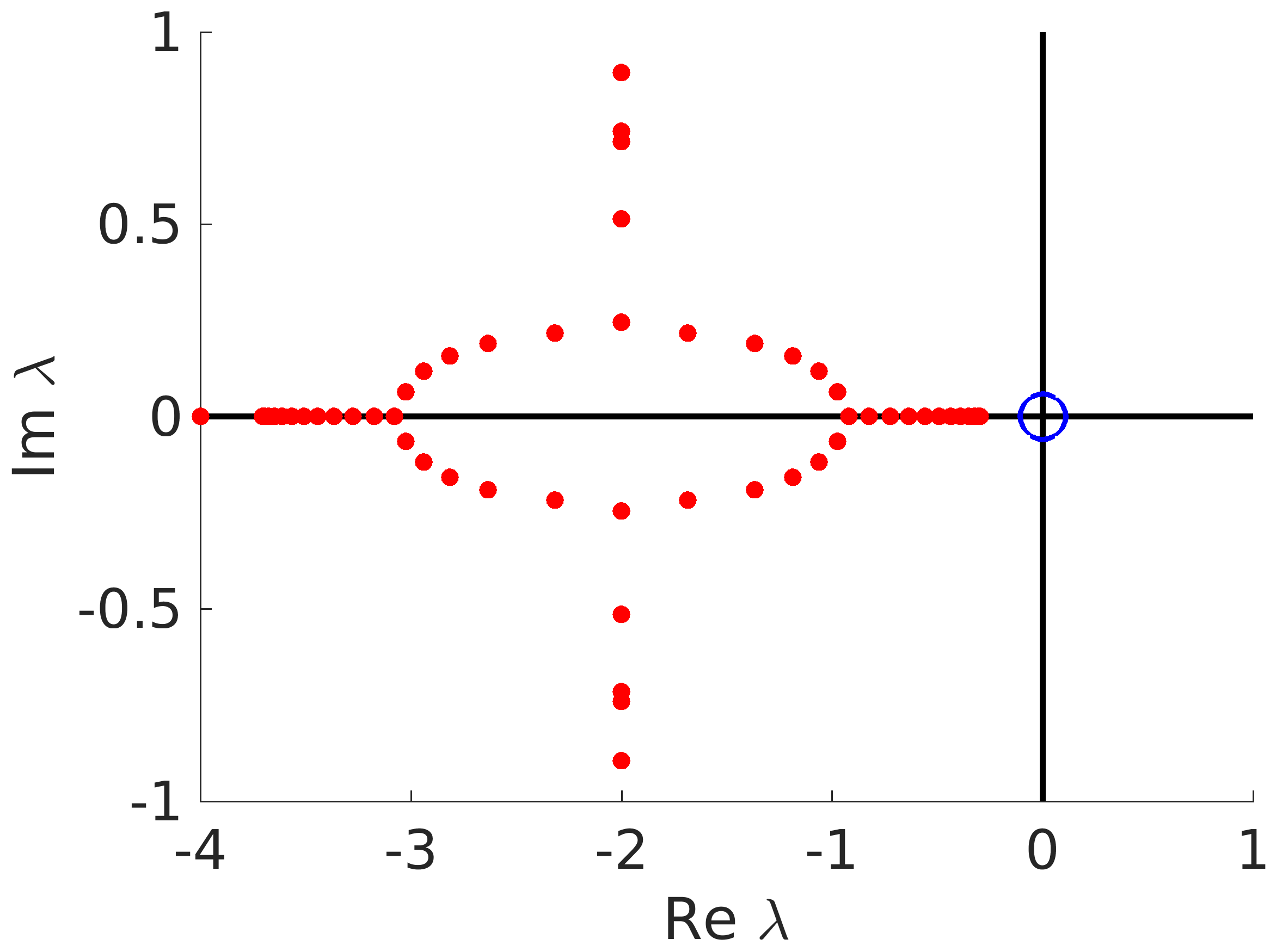
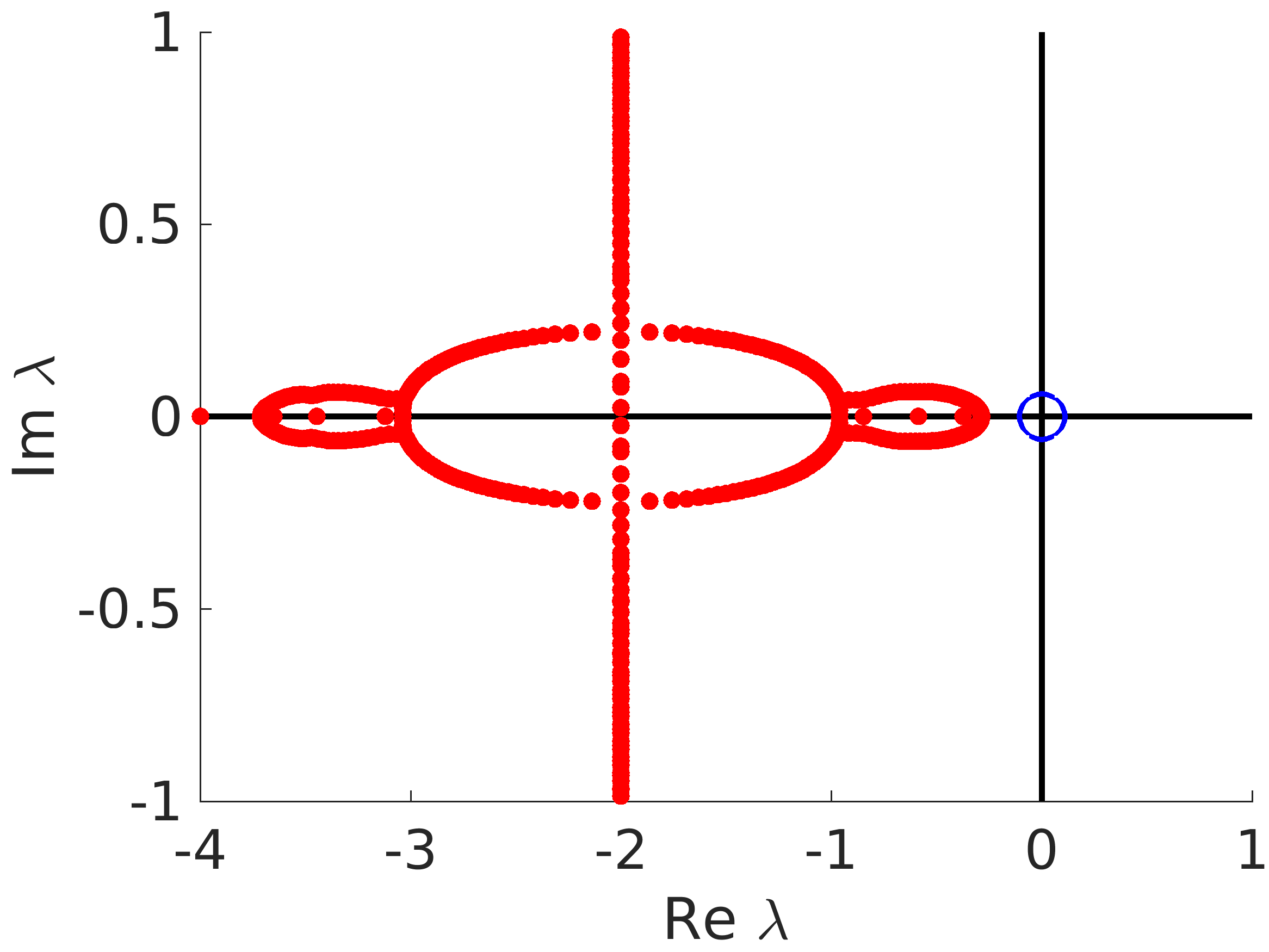
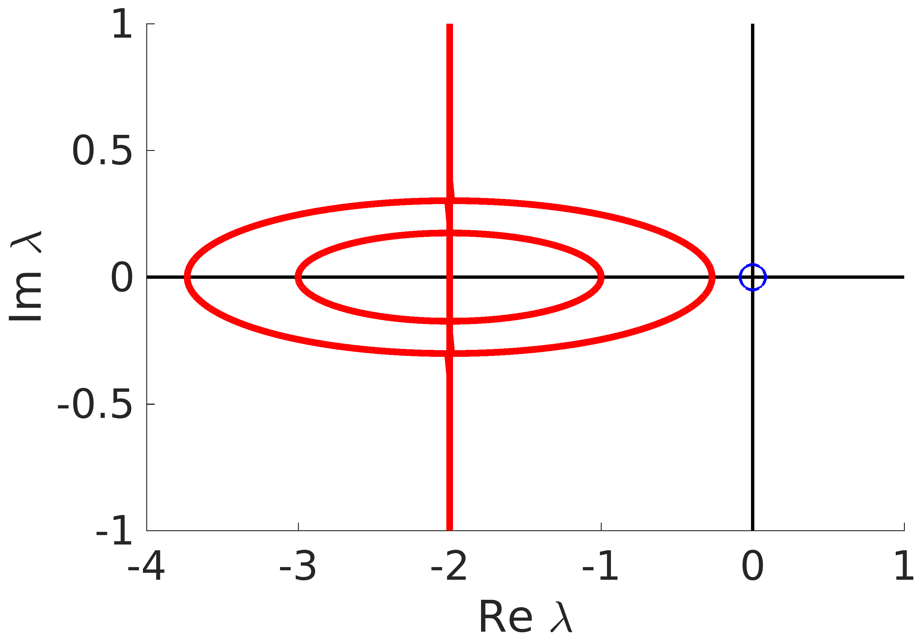
Figure 3.1(a) shows that piece of spectrum which is guaranteed by our propositions at parameter values $\varepsilon=b=\frac{1}{4}$. It is subdivided into point spectrum (blue circle) determined by Proposition 3.3, and essential spectrum (red lines) determined by Proposition 3.5. There may be further isolated eigenvalues. The numerical spectrum of the Nagumo wave on the spatial domain $[-R,R]$ and subject to periodic boundary conditions, is shown in Figure 3.1(b) for $R=50$ and in Figure 3.1(c) for $R=400$. Each of them consists of the approximations of the point spectrum (blue circle) and of the essential spectrum (red dots). The missing line inside the ellipse in Figure 3.1(b) gradually appears numerically when enlarging the spatial domain, see Figure 3.1(c). The second ellipse only develops on even larger domains.

Figure 3.1. Essential spectrum of the Nagumo wave equation for parameters $\varepsilon=b=\frac{1}{4}$ (a) and the numerical spectrum on the spatial domain $[-R,R]$ for $R=50$ (b) and $R=400$ (c).

Example 3.7 (Spectrum of FitzHugh-Nagumo wave system).

As shown in Example 2.4, the FitzHugh-Nagumo wave system (2.32) with coefficient matrices

$$M=\varepsilon I_{2},\quad A=\mathrm{diag}(1,\tfrac{\rho+c_{\star}^{2}\varepsilon}{1+c_{\star}^{2}\varepsilon}),\quad B=I_{2},\quad C=0$$

and parameters from (2.30) has a traveling pulse solution $u_{\star}(x,t)=v_{\star}(x-\mu_{\star}t)$ with

$$\mu_{\star}=\frac{c_{\star}}{k},\quad k=\sqrt{1+c_{\star}^{2}\varepsilon},\quad c_{\star}\approx-0.7892.$$

The profile $v_{\star}$ connects the asymptotic state $v_{\pm}=w_{\pm}$ from (2.31) with itself, i.e. $v_{\star}(\xi)\to v_{\pm}$ as $\xi\to\pm\infty$. The profile $v_{\star}$ and the velocity $\mu_{\star}$ are obtained from the simulation performed in Example 2.4. The FitzHugh-Nagumo nonlinearity $g$ from (2.29) satisfies

$$g(v_{\pm})=\begin{pmatrix}0\\ 0\end{pmatrix}\quad\text{and}\quad Dg(v_{\pm})=\begin{pmatrix}1-\left(v_{\pm,1}\right)^{2}&-1\\ \phi&-b\phi\end{pmatrix}.$$

The dispersion relation for the FitzHugh-Nagumo pulse states that every $\lambda\in\mathbb{C}$ satisfying

(3.14) $$\det\begin{pmatrix}\varepsilon\lambda^{2}+p(\omega)\lambda+q_{1}(\omega)&1\\ -\phi&\varepsilon\lambda^{2}+p(\omega)\lambda+q_{2}(\omega)\end{pmatrix}=0.$$

for some $\omega\in\mathbb{R}$ belongs to $\sigma_{\mathrm{ess}}(\mathcal{P})$, where we used the abbreviations

$$p(\omega)=1-2i\omega\mu_{\star}\varepsilon,\;q_{1}(\omega)=\omega^{2}(1-\mu_{\star}^{2}\varepsilon)-i\omega\mu_{\star}-(1-(v_{\pm,1})^{2}),\;q_{2}(\omega)=\omega^{2}\left(\frac{\rho+c_{\star}^{2}\varepsilon}{1+c_{\star}^{2}\varepsilon}-\mu_{\star}^{2}\varepsilon\right)-i\omega\mu_{\star}+b\phi.$$

Note that (3.14) leads to the quartic problem

$$0 =a_{4}\lambda^{4}+a_{3}\lambda^{3}+a_{2}\lambda^{2}+a_{1}\lambda+a_{0}$$

with $\omega$-dependent coefficients

$$a_{4}=\varepsilon^{2},\quad a_{3}=2\varepsilon p,\quad a_{2}=\varepsilon(q_{1}+q_{2})+p^{2},\quad a_{1}=p(q_{1}+q_{2}),\quad a_{0}=q_{1}q_{2}+\phi.$$

Figure 3.2. Essential spectrum of the FitzHugh-Nagumo wave system for parameters from (2.30) and $\varepsilon=10^{-2}$ (a), the numerical spectrum (b) and both components of the eigenfunction belonging to $\lambda\approx 0$ (c).

Instead of this we solved numerically the quadratic eigenvalue problem (3.14) using parameter continuation with respect to $\omega$. In this way we obtain analytical information about the spectrum of the FitzHugh-Nagumo pulse shown in Figure 3.2(a) (red lines) for $\varepsilon=10^{-2}$. Again part of the point spectrum (blue circle) is determined by Proposition 3.3 and part of the essential spectrum (red lines) by Proposition 3.5. Zooming into the essential spectrum shows that the parabola-shaped structure contains at both ends a loop which is already known from the first order limit case, see [3]. From these results it is obvious that there is again a spectral gap to the imaginary axis, but we have no analytic expression for this gap. The numerical spectrum for periodic boundary conditions is shown in Figure 3.2(b). It consists of the approximations of the point spectrum (blue circle) and of the essential spectrum (red dots). Figure 3.2(c) shows the approximation of both components $w_{1}$ and $w_{2}$ of the eigenfunction $w(\xi)\approx v_{\star,\xi}(\xi)$ belonging to the small eigenvalue $\lambda=1.311\cdot 10^{-10}$ which approximates the eigenvalue $0$. Note that an approximation of $v_{\star}=(v_{\star,1},v_{\star,2})^{T}$ was provided in Figure 2.5(a).

4. First order systems and stability of traveling waves

In this section we transform the original second order damped wave equation (1.1) into a first order system of triple size. To the first order system we then apply stability results from [28] and derive asymptotic stability of traveling waves for the original second order problem and the second order freezing method. Transferring regularity and stability between these two systems requires some care, and we will provide details of the proofs in Appendix A.

4.1. Transformation to first order system and stability with asymptotic phase

In the following we impose the smoothness condition

Assumption 4.1.

The function $f:\mathbb{R}^{3m}\rightarrow\mathbb{R}^{m}$ satisfies $f\in C^{3}(\mathbb{R}^{3m},\mathbb{R}^{m})$

and the following well-posedness condition

Assumption 4.2.

The matrix $M\in\mathbb{R}^{m,m}$ is invertible and $M^{-1}A$ is positive diagonalizable.

Assumption 4.2 implies that there is a (not necessarily unique) positive diagonalizable matrix $N\in\mathbb{R}^{m,m}$ satisfying $N^{2}=M^{-1}A$. Let $\lambda_{1}\geqslant\cdots\geqslant\lambda_{m}>0$ denote the real positive eigenvalues of $N$.

We transform to a first order system by introducing $U=(U_{1},U_{2},U_{3})^{\top}\in\mathbb{R}^{3m}$ via

(4.1) $$U_{1}=u,\quad U_{2}=u_{t}+Nu_{x},\quad U_{3}=u_{t}-Nu_{x}+cu,$$

where $c\in\mathbb{R}$ is an arbitrary constant to be determined later. These variables transform (1.1) into the first order system

(4.2) $$U_{t}=EU_{x}+F(U),$$

with $E\in\mathbb{R}^{3m,3m}$ and $F:\mathbb{R}^{3m}\rightarrow\mathbb{R}^{3m}$ given by

(4.3) $$E= \begin{pmatrix}N&0&0\\ 0&N&0\\ 0&0&-N\end{pmatrix},\quad F(U)=\begin{pmatrix}-cU_{1}+U_{3}\\ \tilde{f}(U)\\ \tilde{f}(U)+cU_{2}\end{pmatrix},$$

$$\tilde{f}(U):= M^{-1}f(U_{1},\frac{1}{2}N^{-1}(U_{2}-U_{3}+cU_{1}),\frac{1}{2}(U_{2}+U_{3}-cU_{1})).$$

Thus we write the second-order Cauchy problem (2.1) as a first-order Cauchy problem for (4.2),

(4.4) $$U_{t}=EU_{x}+F(U),\quad U(\cdot,0)=U_{0}:=(u_{0},v_{0}+Nu_{0,x},v_{0}-Nu_{0,x}+cu_{0})^{\top}.$$

Remark 4.3.

The transformation to a first order system has some arbitrariness and does not influence the results for the second order problem (1.1). The current transformation to a system of dimension $3m$ improves an earlier version [5] of our work which was limited to the semilinear case (1.2). There we used $U_{1}=u,U_{2}=u_{t}-Nu_{x}$ to obtain a system of minimal dimension $2m$. But for this transformation the general nonlinear equation (1.1) does not lead to a semilinear system of type (4.2). The drawback of the non-minimal dimension $3m$ is that extra eigenvalues of the linearized system appear which do not correspond to those of the linearized second order system. The constant $c$ above will be used in Section A.2 to control these extra eigenvalues.

We emphasize that system (4.2) is diagonalizable hyperbolic. More precisely, there is a nonsingular block-diagonal matrix $T\in\mathbb{R}^{3m,3m}$, so that the change of variables $W=T^{-1}U$ transforms (4.2) into diagonal hyperbolic form

(4.5) $$W_{t}=\Lambda_{E}W_{x}+G(W),\quad\Lambda_{E}=T^{-1}ET=\mathrm{diag}(\Lambda,\Lambda,-\Lambda),\quad G(W)=T^{-1}F(TW),$$

where $\Lambda=\mathrm{diag}(\lambda_{1},\ldots,\lambda_{m})$. For systems of type (4.4), (4.5) we have local well-posedness of the Cauchy problem in suitable function spaces such as (see e.g. [26, Sect. 6])

(4.6) $$\mathcal{CH}^{k}(J;\mathbb{R}^{n})=\bigcap_{j=0}^{k}C^{k-j}\bigl{(}J,H^{j}(\mathbb{R},\mathbb{R}^{n})\bigr{)},\quad J\subseteq\mathbb{R}\text{ interval},\;k\in\mathbb{N}_{0},\;n\in\mathbb{N}.$$

Our regularity condition on the traveling wave is as follows:

Assumption 4.4.

The pair $(v_{\star},\mu_{\star})\in C^{2}_{b}(\mathbb{R},\mathbb{R}^{m})\times\mathbb{R}$ satisfies $v_{\star,\xi}\in H^{3}(\mathbb{R},\mathbb{R}^{m})$ and is a non-constant solution of the second order traveling wave equation (1.6) with

$$\lim_{\xi\rightarrow\pm\infty}v_{\star}(\xi)=v_{\pm},\quad\lim_{\xi\rightarrow\pm\infty}v_{\star,\xi}(\xi)=0,\quad f(v_{\pm},0,0)=0.$$

The first order system (4.2) then has a traveling wave

(4.7) $$U_{\star}(x,t)=V_{\star}(x-\mu_{\star}t),\quad V_{\star}:=\begin{pmatrix}v_{\star}\\ (N-\mu_{\star}I_{m})v_{\star,\xi}\\ cv_{\star}-(N+\mu_{\star}I_{m})v_{\star,\xi}\end{pmatrix}\in C^{2}_{b}(\mathbb{R},\mathbb{R}^{m})\times C^{1}_{b}(\mathbb{R},\mathbb{R}^{2m}).$$

The profile $V_{\star}$ solves the equation

(4.8) $$0=(E+\mu_{\star}I_{3m})V_{\star,\xi}+F(V_{\star})$$

and satisfies

(4.9) $$\lim_{\xi\to\pm\infty}V_{\star}(\xi)=V_{\pm}:=(v_{\pm},0,cv_{\pm})\quad\text{and}\quad F(V_{\pm})=0.$$

Our next assumption is

Assumption 4.5.

The matrix $A-\mu_{\star}^{2}M$ is nonsingular.

It guarantees that (1.6) is a regular second order system and that $v_{\star}\in C_{b}^{5}(\mathbb{R},\mathbb{R}^{m})$ which follows from Assumptions 4.1 and 4.4. Further, from $A-\mu_{\star}^{2}M=M(N-\mu_{\star}I_{m})(N+\mu_{\star}I_{m})$ one infers that the matrix $E+\mu_{\star}I_{3m}$ in (4.8) is nonsingular. This will enable us to apply the stability results from [28] which hold for hyperbolic systems where the matrix $E+\mu_{\star}I_{3m}$ is real diagonalizable with nonzero but not necessarily distinct eigenvalues. The condition also ensures that any solution $V_{\star}\in C^{1}_{b}(\mathbb{R},\mathbb{R}^{3m})$ of (4.8) has a first component in $C^{2}_{b}(\mathbb{R},\mathbb{R}^{m})$ which solves the second order traveling wave equation (1.6). Moreover, using the limits from Assumption 4.4 one obtains from (1.6)

(4.10) $$\lim_{\xi\rightarrow\pm\infty}v_{\star,\xi\xi}(\xi)=0.$$

Next, recall the dispersion set (3.6) for the original second order problem

(4.11) $$\sigma_{\mathrm{disp}}(\mathcal{P})=\Bigl{\{}\lambda\in\mathbb{C}:\det\bigl{(}\lambda^{2}A_{2}+\lambda A_{1}^{\pm}(\omega)+A_{0}^{\pm}(\omega)\bigr{)}=0\;\text{for some }\omega\in\mathbb{R},\;\text{and some sign}\;\pm\Bigr{\}},$$

with $A_{0}^{\pm},A_{1}^{\pm},A_{2}$ given in (3.5). We require

Assumption 4.6.

There is $\delta>0$ such that $\mathrm{Re}\,(\sigma_{\mathrm{disp}}(\mathcal{P}))<-\delta$.

Finally, we exclude nonzero eigenvalues in the right half plane.

Assumption 4.7.

The eigenvalue $0$ of $\mathcal{P}$ is simple and there is no other eigenvalue of $\mathcal{P}$ with real part greater than $-\delta$ with $\delta$ given by Assumption 4.6.

With these assumptions our first main result reads:

Theorem 4.8 (Stability with asymptotic phase).

Let Assumptions 4.1 – 4.7 hold. Then, for all $0<\eta<\delta$ there is $\rho>0$ such that for all $u_{0}\in v_{\star}+H^{3}(\mathbb{R},\mathbb{R}^{m})$, $v_{0}\in H^{2}(\mathbb{R},\mathbb{R}^{m})$ with

(4.12) $$\|u_{0}-v_{\star}\|_{H^{3}}+\|v_{0}+\mu_{\star}v_{\star,\xi}\|_{H^{2}}\leq\rho,$$

the Cauchy problem (2.1) has a unique global solution $u\in v_{\star}+\mathcal{CH}^{2}([0,\infty);\mathbb{R}^{m})$. Moreover, there exist $\varphi_{\infty}=\varphi_{\infty}(u_{0},v_{0})$ and $C=C(\eta,\rho)$ satisfying

(4.13) $$|\varphi_{\infty}|\leq C\Bigl{(}\|u_{0}-v_{\star}\|_{H^{3}}+\|v_{0}+\mu_{\star}v_{\star,\xi}\|_{H^{2}}\Bigr{)}$$

and

(4.14) $$\|u(\cdot,t)-v_{\star}(\cdot-\mu_{\star}t-\varphi_{\infty})\|_{H^{2}}+ \|u_{t}(\cdot,t)+\mu_{\star}v_{\star,\xi}(\cdot-\mu_{\star}t-\varphi_{\infty})\|_{H^{1}}$$

$$\leq C\Bigl{(}\|u_{0}-v_{\star}\|_{H^{3}}+\|v_{0}+\mu_{\star}v_{\star,\xi}\|_{H^{2}}\Bigr{)}e^{-\eta t}\quad\forall t\geq 0.$$

The proof will be given in Appendix A. Let us note that the loss of one derivative for the solution when compared to initial data, is typical for hyperbolic stability theorems and results from the theory in [28].

4.2. Stability of the freezing method

Let us first apply the freezing method to the first order system (4.4). We introduce new unknowns $\gamma(t)\in\mathbb{R}$ and $V(\xi,t)\in\mathbb{R}^{3m}$ via the ansatz

(4.15) $$U(x,t) =V(\xi,t),\quad\xi:=x-\gamma(t),\quad x\in\mathbb{R},\,t\geq 0.$$

This formally leads to

(4.16a) $$V_{t} =(E+\mu I_{3m})V_{\xi}+F(V),$$

(4.16b) $$\gamma_{t} =\mu,$$

(4.16c) $$V(\cdot,0) =V_{0}:=U_{0}=(u_{0},v_{0}+Nu_{0,\xi},v_{0}-Nu_{0,\xi}+cu_{0})^{\top},\quad\gamma(0)=0,$$

with $E$ and $F$ from (4.3). In (4.16) we introduced the time-dependent function $\mu(t)\in\mathbb{R}$ for convenience. As before, equation (4.16b) decouples and can be solved in a postprocessing step. One needs an additional algebraic constraint to compensate the extra variable $\mu$. To relate the second order freezing equation (2.5) and the first order version (4.16), we omit the introduction of $\mu_{2}$ in (2.5) and write it in the form

(4.17a) $$Mv_{tt}= (A-\mu^{2}M)v_{\xi\xi}+2\mu Mv_{\xi t}+\mu_{t}Mv_{\xi}+f(v,v_{\xi},v_{t}-\mu v_{\xi}), \xi\in\mathbb{R},\,t\geqslant 0,$$

(4.17b) $$\gamma_{t} =\mu,$$

(4.17c) $$v(\cdot,0) =u_{0},\quad v_{t}(\cdot,0)=v_{0}+\mu(0)u_{0,\xi},\quad\gamma(0)=0.$$

Transforming (4.17) into a first order system by introducing $V=(V_{1},V_{2},V_{3})^{\top}\in\mathbb{R}^{3m}$ via

(4.18) $$V_{1}=v,\quad V_{2}=v_{t}+(N-\mu I_{m})v_{\xi},\quad V_{3}=v_{t}-(N+\mu I_{m})v_{\xi}+cv$$

we again find the system (4.16). As a consequence we obtain the equivalence of the freezing systems for the first and the second order formulation. Henceforth we restrict to the fixed phase condition (2.9) for which we require the following condition.

Assumption 4.9.

The template function $\hat{v}:\mathbb{R}\to\mathbb{R}^{m}$ belongs to $v_{\star}+H^{1}(\mathbb{R},\mathbb{R}^{m})$ and satisfies

(4.19a) $$\langle\hat{v}-v_{\star},\hat{v}_{\xi}\rangle_{L^{2}} =0,$$

(4.19b) $$\langle v_{\star,\xi},\hat{v}_{\xi}\rangle_{L^{2}} \neq 0.$$

Condition (4.19a) implies that (2.8) holds for the fixed phase condition (2.9), so that $(v_{\star},\mu_{\star},0)$ is a stationary solution of (2.18a), (2.18b) (skipping the $\gamma$-equation needed for reconstruction only). Condition (4.19b) specifies some non-degeneracy used in the proof.

Now we are ready to state asymptotic stability (in the sense of Lyapunov) of the steady state $(v_{\star},\mu_{\star},0)$ for the freezing system (2.18) that belongs to the nonlinear wave equation.

Theorem 4.10 (Stability of the freezing method).

Let Assumptions 4.1 – 4.7 hold and consider the phase condition $\psi^{\mathrm{2nd}}(v,v_{t},\mu_{1},\mu_{2})=\langle v-\hat{v},\hat{v}_{\xi}\rangle_{L^{2}}$ with a template function $\hat{v}$ which fulfills the non-degeneracy Assumption 4.9. Then, for all $0<\eta<\delta$ there is $\rho>0$ such that for all $u_{0}\in v_{\star}+H^{3}(\mathbb{R},\mathbb{R}^{m})$, $v_{0}\in H^{2}(\mathbb{R},\mathbb{R}^{m})$ and $\mu_{1}^{0}\in\mathbb{R}$ which satisfy

(4.20) $$\|u_{0}-v_{\star}\|_{H^{3}}+\|v_{0}+\mu_{\star}v_{\star,\xi}\|_{H^{2}}\leq\rho$$

and the consistency conditions (2.12), (2.13), $\langle u_{0}-\hat{v},\hat{v}_{\xi}\rangle_{L^{2}}=0$ the following holds. The freezing system (2.18) has a unique global solution $(v,\mu_{1},\mu_{2},\gamma)\in(v_{\star}+\mathcal{CH}^{2}([0,\infty);\mathbb{R}^{m}))\times C^{1}([0,\infty))\times C([0,\infty))\times C^{2}([0,\infty))$. Moreover, there exists some $C=C(\rho,\eta)>0$ such that the following exponential stability estimate holds

(4.21) $$\|v(\cdot,t)-v_{\star}\|_{H^{2}}+\|v_{t}(\cdot,t)\|_{H^{1}}+|\mu_{1}(t)-\mu_{\star}|\leq C\bigl{(}\|u_{0}-v_{\star}\|_{H^{3}}+\|v_{0}+\mu_{\star}v_{\star,\xi}\|_{H^{2}}\bigr{)}\;e^{-\eta t}\quad\forall t\geq 0.$$

The proof builds on the fact that the original second order version (2.18) and the first order version (4.16) of the freezing method for traveling waves in (1.1) are equivalent in suitable function spaces. This will be detailed in Appendix A

Appendix A Proof of Stability Theorems

In this Appendix we provide a detailed proof of Theorems 4.8 and 4.10.

A.1. Results for first order systems

Let us recall the stability result from [28, Thm.2.5] for first order systems of the general type

(A.1a) $$W_{t}=\Lambda_{E}W_{x}+G(W),\quad\,x\in\mathbb{R},\,t\geq 0,W(x,t)\in\mathbb{R}^{l}$$

(A.1b) $$W(\cdot,0)=W_{0}.$$

The assumptions are

1. The matrix $\Lambda_{E}\in\mathbb{R}^{l,l}$ is diagonal.

2. The nonlinearity $G$ belongs to $C^{3}(\mathbb{R}^{l},\mathbb{R}^{l})$.

3. There exists a traveling wave solution $W(x,t)=W_{\star}(x-\mu_{\star}t)$ of (A.1) such that $W_{\star}\in C^{1}_{b}(\mathbb{R},\mathbb{R}^{l})$, $W_{\star,\xi}\in H^{2}(\mathbb{R},\mathbb{R}^{l})$.

4. The matrix function $Y(\xi)=DG\bigl{(}W_{\star}(\xi)\bigr{)}$ satisfies $\lim_{\xi\to\pm\infty}Y(\xi)=Y_{\pm}$ and $\lim_{\xi\to\pm\infty}Y^{\prime}(\xi)=0$.

5. The matrix $\Lambda_{E}+\mu_{\star}I_{l}\in\mathbb{R}^{l,l}$ is nonsingular.

6. There is $\delta>0$ such that $\mathrm{Re}\,\{s\in\mathbb{C}:s\in\sigma\bigl{(}i\omega(\Lambda_{E}+\mu_{\star}I_{l})+Y_{\pm}\bigr{)}\;\;\text{for some}\;\;\omega\in\mathbb{R}\}\leq-\delta$.

7. The operator $\mathcal{Y}_{\mathrm{1st}}=(\Lambda_{E}+\mu_{\star}I_{l})\partial_{\xi}+Y(\cdot):H^{1}(\mathbb{R},\mathbb{R}^{l})\rightarrow L^{2}(\mathbb{R},\mathbb{R}^{l})$ has the algebraically simple eigenvalue $0$ and satisfies $\sigma_{\mathrm{point}}(\mathcal{Y}_{\mathrm{1st}})\cap\{\mathrm{Re}\,s>-\delta\}=\{0\}$.

Then for every $0<\eta<\delta$ there is $\rho_{0}>0$ so that for all $W_{0}\in W_{\star}+H^{2}(\mathbb{R},\mathbb{R}^{l})$ with $\|W_{0}-W_{\star}\|_{H^{2}}\leq\rho_{0}$ the Cauchy problem (A.1) has a unique global solution $W\in W_{\star}+\mathcal{CH}^{1}([0,\infty);\mathbb{R}^{l})$. Moreover, there is $\varphi_{\infty}=\varphi_{\infty}(W_{0})\in\mathbb{R}$ and $C=C(\eta,\rho_{0})>0$ such that

(A.2) $$|\varphi_{\infty}|\leq C\|W_{0}-W_{\star}\|_{H^{2}},$$

(A.3) $$\|W(\cdot,t)-W_{\star}(\cdot-\mu_{\star}t-\varphi_{\infty})\|_{H^{1}}\leq C\|W_{0}-W_{\star}\|_{H^{2}}e^{-\eta t}\quad\forall t\geq 0.$$

In [28, Thm.2.5] the eigenvalues of $\Lambda_{E}$ are assumed to be in decreasing order. However, this was done for convenience of the proof only, and the result holds verbatim without this ordering. Our goal is to apply the stability result to the system (4.5) where $\Lambda_{E}$ is diagonal but the eigenvalues are not ordered. In the following we show the assumptions (ii)-(vii) for the system (4.5). Our first observation is that instead of checking assumptions (ii)-(vii) for the transformed data $W_{\star}=T^{-1}V_{\star}$, $\Lambda_{E}=T^{-1}ET$ and $G=T^{-1}FT$, it is sufficient to check them for the data $V_{\star}$, $E$ and $F$ of the original system (4.2).

Condition (ii) follows from Assumption 4.1. Moreover, conditon (iii) is a consequence of (4.7) and Assumption 4.4. From (4.3) we obtain (recall $(\star)=(v_{\star},v_{\star,\xi},-\mu_{\star}v_{\star,\xi})$)

(A.4) $$Z=DF(V_{\star})=\begin{pmatrix}-cI_{m}&0&I_{m}\\ \Phi_{1}&\Phi_{2}&\Phi_{3}\\ \Phi_{1}&\Phi_{2}+cI_{m}&\Phi_{3}\end{pmatrix},\quad\begin{pmatrix}\Phi_{1}\\ \Phi_{2}\\ \Phi_{3}\end{pmatrix}:=\begin{pmatrix}M^{-1}D_{1}f(\star)-c\Phi_{3}\\ \frac{1}{2}M^{-1}(D_{2}f(\star)N^{-1}+D_{3}f(\star))\\ \frac{1}{2}M^{-1}(-D_{2}f(\star)N^{-1}+D_{3}f(\star))\end{pmatrix}.$$

By Assumption 4.4 the limit is given by (recall $(\pm)=(v_{\pm},0,0)$)

(A.5) $$Z_{\pm}=\lim_{\xi\rightarrow\pm\infty}Z(\xi)=\begin{pmatrix}-cI_{m}&0&I_{m}\\ \Phi^{\pm}_{1}&\Phi^{\pm}_{2}&\Phi^{\pm}_{3}\\ \Phi^{\pm}_{1}&\Phi^{\pm}_{2}+cI_{m}&\Phi^{\pm}_{3}\end{pmatrix},\quad\begin{pmatrix}\Phi^{\pm}_{1}\\ \Phi^{\pm}_{2}\\ \Phi^{\pm}_{3}\end{pmatrix}:=\begin{pmatrix}M^{-1}D_{1}f(\pm)-c\Phi_{3}^{\pm}\\ \frac{1}{2}M^{-1}(D_{2}f(\pm)N^{-1}+D_{3}f(\pm))\\ \frac{1}{2}M^{-1}(-D_{2}f(\pm)N^{-1}+D_{3}f(\pm))\end{pmatrix}.$$

Differentiating (A.4) w.r.t. $\xi$ and using Assumption 4.4 as well as (4.10) then shows $Z^{\prime}(\xi)\rightarrow 0$ as $\xi\rightarrow\pm\infty$. Further, condition (v) follows from Assumption 4.5 as has been noted in Section 4. The conditions (vi) and (vii) are discussed in the next subsection.

A.2. Spectral relations of first and second order problems

We transfer the spectral properties of the original second order problem (1.1) to the first order problem (4.2) and vice versa. Throughout this section we impose Assumptions 4.1, 4.2, 4.4 and define $V_{\star}$ by (4.7).

By Definition 3.1, the spectral problem for the second order problem (1.1), considered in a co-moving frame, is given by the solvability properties of

$$\mathcal{P}(\lambda):H^{2}(\mathbb{R},\mathbb{C}^{m})\to L^{2}(\mathbb{R},\mathbb{C}^{m}),\quad\text{defined by \eqref{equ:4.1}}.$$

The analog for the first order formulation (4.2) is the first order differential operator

(A.6) $$\mathcal{P}_{\mathrm{1st}}(\lambda) :H^{1}(\mathbb{R},\mathbb{C}^{3m})\to L^{2}(\mathbb{R},\mathbb{C}^{3m})\;\text{ given by}$$

$$\mathcal{P}_{\mathrm{1st}}(\lambda) =\lambda I_{3m}-\mathcal{Z}_{\mathrm{1st}},\quad\mathcal{Z}_{\mathrm{1st}}=(E+\mu_{\star}I_{3m})\partial_{\xi}+Z(\cdot),$$

obtained by linearizing (4.2) in the co-moving frame about the traveling wave $V_{\star}$. Introducing the first order operators

(A.7) $$\mathcal{P}_{-N}(\lambda)=\lambda-(N+\mu_{\star}I_{m})\partial_{\xi},\quad\mathcal{P}_{+N}(\lambda)=\lambda+(N-\mu_{\star}I_{m})\partial_{\xi},$$

we may write $\mathcal{P}_{\mathrm{1st}}(\lambda)$ as a block operator

(A.8) $$\mathcal{P}_{\mathrm{1st}}(\lambda)=\begin{pmatrix}\mathcal{P}_{-N}(\lambda)+cI_{m}&0&-I_{m}\\ -\Phi_{1}&\mathcal{P}_{-N}(\lambda)-\Phi_{2}&-\Phi_{3}\\ -\Phi_{1}&-\Phi_{2}-cI_{m}&\mathcal{P}_{+N}(\lambda)-\Phi_{3}\end{pmatrix}.$$

Finally, it is convenient to introduce the normalized operator polynomial

$$\tilde{\mathcal{P}}(\lambda)=M^{-1}\mathcal{P}(\lambda),\quad\lambda\in\mathbb{C},$$

which has exactly the same spectrum as $\mathcal{P}(\lambda)$. The key to the relation of spectra is the following factorization

(A.9) $$\begin{pmatrix}0&0&I_{m}\\ 0&I_{m}&-I_{m}\\ I_{m}&0&0\end{pmatrix}\mathcal{P}_{\mathrm{1st}}(\lambda)=\begin{pmatrix}\tilde{\mathcal{P}}(\lambda)&-\Phi_{2}-cI_{m}&\mathcal{P}_{+N}(\lambda)-\Phi_{3}\\ 0&\mathcal{P}_{-N}(\lambda)+cI_{m}&-\mathcal{P}_{+N}(\lambda)\\ 0&0&-I_{m}\end{pmatrix}\begin{pmatrix}I_{m}&0&0\\ -\mathcal{P}_{+N}(\lambda)&I_{m}&0\\ -\mathcal{P}_{-N}(\lambda)-cI_{m}&0&I_{m}\end{pmatrix}.$$

This follows from (A.4) and (A.8) by a straightforward but somewhat lengthy calculation. The factorization (A.9) is motivated by the equivalence notion for matrix polynomials (see e.g. [13, Chapter S1.6]).

Let us recall a well-known result on Fredholm properties for first order operators from Palmer [25]:

Proposition A.1.

Consider a first order system

(A.10) $$(\partial_{\xi}-Q(\xi))V=R\in L^{2}(\mathbb{R},\mathbb{C}^{N}),$$

where the matrix-valued function $Q:\mathbb{R}\rightarrow\mathbb{C}^{N,N}$ is continuous and has limits

(A.11) $$Q_{\pm}=\lim_{\xi\rightarrow\pm\infty}Q(\xi).$$

Further assume that $Q_{\pm}$ have no eigenvalues on the imaginary axis. Then the operator

$$\mathcal{Q}=\partial_{\xi}-Q(\cdot):H^{1}(\mathbb{R},\mathbb{C}^{N})\rightarrow L^{2}(\mathbb{R},\mathbb{C}^{N})$$

is Fredholm of index $\dim E_{+}^{s}-\dim E_{-}^{s}$, where $E_{\pm}^{s}\subseteq\mathbb{C}^{N}$ is the stable subspace of $Q_{\pm}$ (i.e. the maximal invariant subspace associated with eigenvalues of negative real part).

A consequence of this result for parametrized systems is the following

Proposition A.2.

Consider a first order system

(A.12) $$\mathcal{Q}(\lambda)V=(\partial_{\xi}-Q(\xi,\lambda))V=R\in L^{2}(\mathbb{R},\mathbb{C}^{l}),$$

with a matrix polynomial $Q(\xi,\lambda)=\sum_{j=0}^{q}Q_{j}(\xi)\lambda^{j}$, $Q_{j}\in C(\mathbb{R},\mathbb{C}^{l,l})$. Assume that the limits $\lim_{\xi\rightarrow\pm\infty}Q_{j}(\xi)=Q_{j}^{\pm}$ exist and let $Q^{\pm}(\lambda)=\sum_{j=0}^{q}Q_{j}^{\pm}\lambda^{j}$. Then the dispersion set

(A.13) $$\sigma_{\mathrm{disp}}(\mathcal{Q})=\{\lambda\in\mathbb{C}:\det(i\omega I-Q^{\pm}(\lambda))=0\;\text{for some}\;\omega\in\mathbb{R}\;\text{and some sign}\;\pm\}$$

is contained in the essential spectrum $\sigma_{\mathrm{ess}}(\mathcal{Q})$. For $\lambda\notin\sigma_{\mathrm{disp}}(\mathcal{Q})$, the operator $\mathcal{Q}(\lambda):H^{1}(\mathbb{R},\mathbb{C}^{l})\rightarrow L^{2}(\mathbb{R},\mathbb{C}^{l})$ is Fredholm of index $\dim E_{+}^{s}(\lambda)-\dim E_{-}^{s}(\lambda)$ where $E_{\pm}^{s}(\lambda)$ denotes the stable subspace of $Q^{\pm}(\lambda)$.

This result may be found in [19, Theorem 3.1.13] (note that the dispersion set is called the Fredholm border there).

If we replace $\partial_{\xi}$ by $i\omega$ and let $\xi\rightarrow\pm\infty$ in (A.9) then the left and right factors in (A.9) are $\lambda$-dependent matrices with a constant determinant (see the equivalence notion of matrix polynomials in [13, Chapter S1.6]). Hence the dispersion set of the first order operator $\mathcal{P}_{\mathrm{1st}}(\lambda)$ is completely determined by the dispersion set (3.7) of the second order operator $\tilde{\mathcal{P}}(\lambda)$ and the first order operator $\mathcal{P}_{-N}(\lambda)+cI_{m}$. Since $N+\mu_{\star}I_{m}$ has nonzero real eigenvalues $\lambda_{j}+\mu_{\star},j=1,\ldots,m$ by (4.5) we find from Propositions A.1 and A.2

$$\sigma(\mathcal{P}_{-N}+cI_{m})=\sigma_{\mathrm{disp}}(\mathcal{P}_{-N}+cI_{m})=\{c+(\lambda_{j}+\mu_{\star})i\omega:\omega\in\mathbb{R},j=1,\ldots,m\}=c+i\mathbb{R}.$$

This yields the following result.

Proposition A.3.

The dispersion sets satisfy

(A.14) $$\sigma_{\mathrm{disp}}(\mathcal{P}_{\mathrm{1st}})=\sigma_{\mathrm{disp}}(\mathcal{P})\cup(c+i\mathbb{R}).$$

This proposition leads to a proper choice of the shift parameter $c$. Taking $c<-\delta$ , condition (vi) immediately follows from Assumption 4.6. The following proposition relates the point spectra of the second order operator $\mathcal{P}$ and the first order operator $\mathcal{P}_{\mathrm{1st}}$ to each other.

Proposition A.4.

The following assertions hold:

1. There exists a $\lambda_{\star}>c$ such that $\sigma_{\mathrm{disp}}(\mathcal{P}_{\mathrm{1st}})\cap[\lambda_{\star},\infty)=\emptyset$.

2. Let $\rho_{+}$ be the connected component of $\{\lambda\in\mathbb{C}:\mathrm{Re}\,\lambda>c\}\setminus\sigma_{\mathrm{disp}}(\mathcal{P}_{\mathrm{1st}})$ containing $[\lambda_{\star},\infty)$. Then the operator $\mathcal{P}_{\mathrm{1st}}(\lambda):H^{1}(\mathbb{R},\mathbb{C}^{2m})\to L^{2}(\mathbb{R},\mathbb{C}^{2m})$ is Fredholm of index $0$ for all $\lambda\in\rho_{+}$.

3. The point spectra of $\mathcal{P}_{\mathrm{1st}}$ and $\mathcal{P}(\lambda):H^{2}(\mathbb{R},\mathbb{C}^{m})\to L^{2}(\mathbb{R},\mathbb{C}^{m})$ in $\rho_{+}$ coincide, i.e.

   (A.15) $$\sigma_{\mathrm{point}}(\mathcal{P})\cap\rho_{+}=\sigma_{\mathrm{point}}(\mathcal{P}_{\mathrm{1st}})\cap\rho_{+}.$$

   Eigenvalues in these sets have the same geometric and maximum partial multiplicity.

Let us first note that this proposition implies condition (vii). For the choice $c<-\delta$ the set $\rho_{+}$ contains $\{\mathrm{Re}\,\lambda>-\delta\}$ by Assumption 4.6 and Proposition A.3. Condition (vii) is then a consequence of Assumption 4.7 and assertion (c) of Proposition A.4.

Proof.

Using Assumption 4.5 we can rewrite the operator from (A.6) as follows

$$\mathcal{P}_{\mathrm{1st}}(\lambda)=-(E+\mu_{\star}I_{3m})(\partial_{\xi}-(E+\mu_{\star}I_{3m})^{-1}(\lambda I_{3m}-DF(V_{\star}))).$$

The matrix $(E+\mu_{\star}I_{3m})^{-1}$ is hyperbolic by Assumption 4.5 and this property persists for the matrix $(E+\mu_{\star}I_{3m})^{-1}(\lambda I_{3m}-DF(V_{\pm}))$ for $\lambda\geq\lambda_{\star}$ sufficiently large, independently of the sign $\pm$ and with the same number of stable and unstable eigenvalues. Therefore $\mathcal{P}_{\mathrm{1st}}(\lambda)$ is Fredholm of index $0$ by Proposition A.2 for $\lambda\in[\lambda_{\star},\infty)$. Since the Fredholm index is continuous in $\rho_{+}$ and can only change at $\sigma_{\mathrm{disp}}(\mathcal{P}_{\mathrm{1st}})$ or at $c+i\mathbb{R}$, assertion (b) also follows.

Consider an eigenvalue $\lambda_{0}\in\sigma_{\mathrm{point}}(\mathcal{P}_{\mathrm{1st}})\cap\rho_{+}$ with eigenfunction $V=(V_{1},V_{2},V_{3})^{\top}\in H^{1}(\mathbb{R},\mathbb{C}^{3m}),V\neq 0$. The first block equation reads $(\mathcal{P}_{-N}(\lambda_{0})+cI_{m})V_{1}=V_{3}\in H^{1}$ from which we infer $V_{1}\in H^{2}(\mathbb{R},\mathbb{C}^{m})$. In the following let us write the factorization (A.9) in the short form

(A.16) $$T_{1}\mathcal{P}_{\mathrm{1st}}(\lambda)=R(\lambda)T_{2}(\lambda)$$

and apply it to $V$. Then $W(\lambda_{0}):=T_{2}(\lambda_{0})V$ satisfies $R(\lambda_{0})W(\lambda_{0})=0$, and from the triangular structure of $R$ and the invertibility of $\mathcal{P}_{-N}(\lambda_{0})+cI_{m}$ we obtain $W_{3}=0,W_{2}=0$ as well as $\tilde{\mathcal{P}}(\lambda_{0})V_{1}=\tilde{\mathcal{P}}(\lambda_{0})W_{1}=0$. If $V_{1}=0$ then $V_{2}=0,V_{3}=0$ follows from $W_{2}=0,W_{3}=0$, hence $V_{1}\neq 0$. In a similar manner, if $\tilde{\mathcal{P}}(\lambda_{0})W_{1}=0$ for some $W_{1}\in H^{2}(\mathbb{R},\mathbb{C}^{m}),W_{1}\neq 0$ then $\mathcal{P}_{\mathrm{1st}}(\lambda_{0})V=0$ and $V\neq 0$ for $V=T_{2}(\lambda_{0})^{-1}\begin{pmatrix}W_{1}&0&0\end{pmatrix}^{\top}$. By the same argument the null spaces $\mathcal{N}(\mathcal{P}_{\mathrm{1st}}(\lambda_{0}))$ and $\mathcal{N}(\tilde{\mathcal{P}}(\lambda_{0})$) have equal dimension.

Finally, consider a root polynomial $V(\lambda)=\sum_{j=0}^{n}V_{[j]}(\lambda-\lambda_{0})^{j}$ with $V_{[j]}\in H^{1}(\mathbb{R},\mathbb{C}^{3m})$ satisfying

$$V(\lambda_{0})=V_{[0]}\neq 0,\quad(\mathcal{P}_{\mathrm{1st}}V)^{(\nu)}(\lambda_{0})=0,\nu=0,\ldots,n-1.$$

As above we find $V_{[0],1}\in H^{2}(\mathbb{R},\mathbb{C}^{m})$, $V_{[0],1}\neq 0$ and then by induction $V_{[j],1}\in H^{2}(\mathbb{R},\mathbb{C}^{m}),j=1,\ldots,n$ from the equations

$$\nu!\ \mathcal{P}_{\mathrm{1st}}(\lambda_{0})V_{[\nu]}=-\sum_{\ell=1}^{\nu}{\nu\choose\ell}\mathcal{P}_{\mathrm{1st}}^{(\ell)}(\lambda_{0})V^{(\nu-\ell)}(\lambda_{0}).$$

Note that the right-hand side is in $H^{1}(\mathbb{R},\mathbb{C}^{3m})$ since the $\lambda$-derivative of $\mathcal{P}_{\mathrm{1st}}$ is $I_{3m}$. Setting $W(\lambda)=T_{2}(\lambda)V(\lambda)$ then leads via (A.16) to

$$(RW)^{(\nu)}(\lambda_{0})=0,\nu=0,\ldots,n-1.$$

Working backwards through the components of this equation gives $W^{(\nu)}_{k}(\lambda_{0})=0,\nu=0,\ldots,n-1$ for $k=3,2$, and therefore,

$$0=(\tilde{\mathcal{P}}W_{1})^{(\nu)}(\lambda_{0}),\nu=0,\ldots,n-1,$$

with $W_{1}(\lambda_{0})=V_{1}(\lambda_{0})\neq 0$.

Conversely, let $W_{1}(\lambda)=\sum_{j=0}^{n-1}(\lambda-\lambda_{0})^{j}W_{[j],1}$ be a root polynomial of $\tilde{\mathcal{P}}$ in $H^{2}(\mathbb{R},\mathbb{C}^{m})$ with $W_{[0],1}\neq 0$. Then we set $W(\lambda)=\begin{pmatrix}W_{1}(\lambda)&0&0\end{pmatrix}^{\top}$ and find that

$$V(\lambda)=T_{2}(\lambda)^{-1}W(\lambda)=\begin{pmatrix}W_{1}(\lambda)&\mathcal{P}_{+N}(\lambda)W_{1}(\lambda)&(-\mathcal{P}_{-N}(\lambda)+cI_{m})W_{1}(\lambda)\end{pmatrix}^{\top}\in H^{1}(\mathbb{R},\mathbb{C}^{3m})$$

satisfies $V(\lambda_{0})\neq 0$ and

$$T_{1}(\mathcal{P}_{\mathrm{1st}}V)^{(\nu)}(\lambda_{0})=(RW)^{(\nu)}(\lambda_{0})=0,\nu=0,\ldots,n-1.$$

∎

A.3. Stability for the second order system

In the following we consider the Cauchy problem (4.4) and recall the function spaces (4.6). We need two auxiliary results. The first one is regularity of solutions with respect to source terms taken from the theory of linear first order systems (see [26, Cor.2.2.2]).

Lemma A.5.

Consider a first order system

(A.17) $$u_{t}=A_{1}u_{x}+B_{1}u+r,\quad u(x,0)=u_{0}(x),\quad x\in\mathbb{R},t\geq 0,$$

where $A_{1}\in\mathbb{R}^{l,l}$ is real diagonalizable and $B_{1}\in\mathbb{R}^{l,l}$. If $u_{0}\in H^{k}(\mathbb{R},\mathbb{R}^{l})$ for some $k\geq 1$ and $r\in\mathcal{CH}^{k-1}([0,\infty);\mathbb{R}^{l})$ then the system (A.17) has a unique solution in $u\in\mathcal{CH}^{k}([0,\infty);\mathbb{R}^{l})$.

The second one concerns commuting weak and strong derivatives with respect to space and time.

Lemma A.6.

For $u\in C^{1}([0,\infty);H^{1}(\mathbb{R},\mathbb{R}^{l})))$ let $\frac{d}{dt}u\in C^{0}([0,\infty);H^{1}(\mathbb{R},\mathbb{R}^{l})))$ be its time derivative and let $\frac{\partial}{\partial x}u(\cdot,t)$ be its weak space derivative pointwise in $t\in[0,\infty)$. Then $\frac{\partial}{\partial x}u\in C^{1}([0,\infty);L^{2}(\mathbb{R},\mathbb{R}^{l}))$ and its time derivative agrees with the weak spatial derivative of $\frac{d}{dt}u$ evaluated pointwise in $t\in[0,\infty)$, i.e.

(A.18) $$\frac{d}{dt}(\frac{\partial}{\partial x}u)=\frac{\partial}{\partial x}(\frac{d}{dt}u).$$

Proof.

Let $t,t+h\in[0,\infty)$ with $h\neq 0$ and note that

$$\|\frac{1}{h}(\frac{\partial}{\partial x}u(\cdot,t+h)-\frac{\partial}{\partial x}u(\cdot,t))-\frac{\partial}{\partial x}(\frac{d}{dt}u(\cdot,t))\|_{L^{2}}\leq\|\frac{1}{h}(u(\cdot,t+h)-u(\cdot,t))-\frac{d}{dt}u(\cdot,t)\|_{H^{1}},$$

where the right-hand side converges to zero as $h\rightarrow 0$ by assumption. Therefore, the derivative $\frac{d}{dt}(\frac{\partial}{\partial x}u)$ exists in $L^{2}(\mathbb{R},\mathbb{R}^{l})$ for all $t\in[0,\infty)$ and coincides with $\frac{\partial}{\partial x}(\frac{d}{dt}u)\in C^{0}([0,\infty);L^{2}(\mathbb{R},\mathbb{R}^{l}))$. ∎

Remark A.7.

In a loose sense we may write (A.18) as commuting partial dervatives $u_{xt}=u_{tx}$. However, this equality has to be interpreted with care since time and space derivatives are taken with respect to different norms.

We proceed with the proof of Theorem 4.8 by using the stability statements from (A.2),(A.3). From (4.7) and (4.16c) we obtain

(A.19) $$V_{0}-V_{\star}=(u_{0}-v_{\star},v_{0}+\mu_{\star}v_{\star,\xi}+N(u_{0,\xi}-v_{\star,\xi}),v_{0}+\mu_{\star}v_{\star,\xi}-N(u_{0,\xi}-v_{\star,\xi})+c(u_{0}-v_{\star}))^{\top}.$$

Therefore, we have a constant $C_{\star}=C_{\star}(c,\|N\|)$ with

(A.20) $$\|V_{0}-V_{\star}\|_{H^{2}}\leq C_{\star}(\|u_{0}-v_{\star}\|_{H^{3}}+\|v_{0}+\mu_{\star}v_{\star,\xi}\|_{H^{2}})\leq C_{\star}\rho,$$

and we take $\rho$ such that $C_{\star}\rho\leq\rho_{0}$. Let $V\in V_{\star}+\mathcal{CH}^{1}([0,\infty);\mathbb{R}^{3m})$ be the unique solution of (4.4) for $\|V_{0}-V_{\star}\|_{H^{2}}\leq\rho_{0}$. The first component $V_{1}$ satisfies

(A.21) $$V_{1,t}=NV_{1,x}-cV_{1}+V_{3},\quad V_{1}(\cdot,0)=u_{0},$$

so that $\tilde{V}_{1}=V_{1}-v_{\star}$ solves the Cauchy problem

$$\tilde{V}_{1,t}=N\tilde{V}_{1,x}-c\tilde{V}_{1}+V_{3}-V_{\star,3}-\mu_{\star}v_{\star,x},\quad\tilde{V}_{1}(\cdot,0)=u_{0}-v_{\star}.$$

Then Lemma A.5 applies with $k=2,A_{1}=N,B_{1}=-cI_{m}$, $r=V_{3}-V_{\star,3}-\mu_{\star}v_{\star,x}$ and yields $\tilde{V}_{1}=V_{1}-v_{\star}\in\mathcal{CH}^{2}([0,\infty);\mathbb{R}^{m})$. By Lemma A.6 we obtain $\tilde{V}_{1,x}\in C^{1}([0,\infty);L^{2}(\mathbb{R},\mathbb{R}^{m}))$ as well as $\tilde{V}_{1,tx}=\tilde{V}_{1,xt}\in C^{0}([0,\infty);L^{2}(\mathbb{R},\mathbb{R}^{m}))$. Since $v_{\star}$ does not depend on $t$ we also have $V_{1,tx}=\tilde{V}_{1,tx}=\tilde{V}_{1,xt}=V_{1,xt}$. For the same reason $\tilde{V}_{1,tt}=V_{1,tt}\in C^{0}([0,\infty);L^{2}(\mathbb{R},\mathbb{R}^{m}))$, and $\tilde{V}_{1,xx}=(V_{1}-v_{\star})_{xx}\in C^{0}([0,\infty);L^{2}(\mathbb{R},\mathbb{R}^{m}))$ implies $V_{1,xx}\in C^{0}([0,\infty);L^{2}(\mathbb{R},\mathbb{R}^{m}))$ since $v_{\star,xx}\in H^{2}(\mathbb{R},\mathbb{R}^{m})$ by Assumption 4.4. Thus we can take space and time derivative of equation (A.21) and obtain from the third row of (4.4)

(A.22) $$\tilde{f}(V)= V_{3,t}+NV_{3,x}-cV_{2}$$

$$= V_{1,tt}-N^{2}V_{1,xx}-NV_{1,xt}+cV_{1,t}+NV_{1,tx}+cNV_{1,x}-cV_{2}$$

$$= V_{1,tt}-N^{2}V_{1,xx}-c(V_{2}-V_{1,t}-NV_{1,x}).$$

Next introduce the functions

(A.23) $$W_{2}=V_{2}-V_{1,t}-NV_{1,x},\quad W_{3}=V_{3}-V_{1,t}+NV_{1,x}-cV_{1}.$$

Using (A.22), the last two rows of (4.4) and Lemma A.6 again, these functions solve the hyperbolic system

(A.24) $$W_{2,t}-NW_{2,x}= V_{2,t}-V_{1,tt}-NV_{1,xt}-NV_{2,x}+NV_{1,tx}+N^{2}V_{1,xx}=-cW_{2}$$

$$W_{3,t}+NW_{3,x}= V_{3,t}+NV_{3,x}-V_{1,tt}-NV_{1,tx}+NV_{1,xt}+N^{2}V_{1,xx}-cV_{1,t}-cNV_{1,x}$$

$$= \tilde{f}(V)+cV_{2}-(\tilde{f}(V)+cW_{2})-c(V_{1,t}+NV_{1,x})=0.$$

Using from (4.4) the initial data and the differential equation at $t=0$ one finds that $W_{2}(\cdot,0)=0$, $W_{3}(\cdot,0)=0$. Since (A.24) with homogeneous initial data has only the trivial solution we conclude $W_{2}\equiv 0,W_{3}\equiv 0$. Therefore, by setting $u=V_{1}$, equations (A.22) and (A.23) finally lead to

$$u_{tt}-N^{2}u_{xx}=\tilde{f}(V)=M^{-1}f(V_{1},\frac{1}{2}N^{-1}(V_{2}-V_{3}+cV_{1}),\frac{1}{2}(V_{2}+V_{3}-cV_{1}))=M^{-1}f(u,u_{x},u_{t}).$$

Applying (A.2) and using (A.20) we obtain that the asymptotic phase $\varphi_{\infty}$ satisfies an estimate

$$|\varphi_{\infty}|\leq C\|V_{0}-V_{\star}\|_{H^{2}}\leq CC_{\star}(\|u_{0}-v_{\star}\|_{H^{3}}+\|v_{0}+\mu_{\star}v_{\star,x}\|_{H^{2}}).$$

Further, we have for $t\geq 0$ the stability estimate

$$\|V(\cdot,t)-V_{\star}(\cdot-\mu_{\star}t-\varphi_{\infty})\|_{H^{1}}\leq CC_{\star}(\|u_{0}-v_{\star}\|_{H^{3}}+\|v_{0}+\mu_{\star}v_{\star,x}\|_{H^{2}})e^{-\eta t},$$

where $C$ depends only on $\eta,\rho$. From this we retrieve the estimate (4.13) for the original variables by taking the $H^{1}$-norm of the equation

(A.25) $$V(\cdot,t)-V_{\star}(\cdot-\mu_{\star}t-\varphi_{\infty})=\begin{pmatrix}I_{m}&0&0\\ 0&N&I_{m}\\ cI_{m}&-N&I_{m}\end{pmatrix}\begin{pmatrix}u(\cdot,t)-v_{\star}(\cdot-\mu_{\star}t-\varphi_{\infty})\\ u_{x}(\cdot,t)-v_{\star,x}(\cdot-\mu_{\star}t-\varphi_{\infty})\\ u_{t}(\cdot,t)+\mu_{\star}v_{\star,x}(\cdot-\mu_{\star}t-\varphi_{\infty})\end{pmatrix}$$

and using that the left factor of the right-hand side is invertible.

A.4. Lyapunov stability of the freezing method

Let us first recall from [28, Thm.2.7] the stability theorem for the freezing method associated with the first order formulation (A.1)

(A.26a) $$W_{t}=\Lambda_{E}W_{x}+G(W)+\mu W_{x},\quad\,x\in\mathbb{R},\,t\geq 0,W(x,t)\in\mathbb{R}^{l}$$

(A.26b) $$W(\cdot,0)=W_{0},$$

(A.26c) $$\Psi(W-\hat{W})=0.$$

Here, $\Psi:L^{2}(\mathbb{R},\mathbb{R}^{l})\rightarrow\mathbb{R}$ is a linear functional and $\hat{W}:\mathbb{R}\rightarrow\mathbb{R}^{l}$ is a template function for which we assume

1. $\Psi(W_{\star,\xi})\neq 0$, $\Psi$ is bounded,

2. $\hat{W}\in W_{\star}+H^{1}(\mathbb{R},\mathbb{R}^{l})$ and $\Psi(W_{\star}-\hat{W})=0$.

Under the combined assumptions of (i)-(vii) and (viii), (ix) the result is the following. For every $0<\eta<\delta$ there exists $\rho_{0}>0$ such that for all initial data $W_{0}\in W_{\star}+H^{2}(\mathbb{R},\mathbb{R}^{l})$ with $\|W_{0}-W_{\star}\|_{H^{2}}\leq\rho_{0}$ the system (A.26) has a unique solution $(W,\mu)$ in $\Big{(}W_{\star}+\mathcal{CH}^{1}([0,\infty);\mathbb{R}^{3m})\Big{)}\times C([0,\infty),\mathbb{R})$. Moreover, there is a constant $C=C(\eta)$ such that the solution satisfies

(A.27) $$\|W(t)-W_{\star}\|_{H^{1}}+|\mu(t)-\mu_{\star}|\leq C(\eta)\|W_{0}-W_{\star}\|_{H^{2}}e^{-\eta t},\quad t\geq 0.$$

We apply this to the frozen version of (4.5) with the functional $\Psi$ and the function $\hat{W}$ defined by

(A.28) $$\hat{V}= \begin{pmatrix}\hat{v}&0&0\end{pmatrix}^{\top},\hat{W}=T^{-1}\hat{V},$$

$$\Psi(W-\hat{W})= \langle T(W-\hat{W}),T\hat{W}_{\xi}\rangle_{L^{2}}.$$

While conditions (i)-(vii) have already been verified, the conditions (viii) and (ix) easily follow from Assumption 4.9 and the settings $W_{\star}=T^{-1}V_{\star}$ and (4.7). Thus the above result applies. By $(W,\mu)$ we denote the unique solution of (A.26) for $\|W_{0}-W_{\star}\|_{H^{2}}\leq\rho_{0}$, and we let $(V=TW,\mu)$ be the unique solution in $\Big{(}V_{\star}+\mathcal{CH}^{1}([0,\infty);\mathbb{R}^{3m})\Big{)}\times C([0,\infty),\mathbb{R})$ of the transformed equation

(A.29a) $$V_{t}=EV_{\xi}+F(V)+\mu V_{\xi},\quad\,\xi\in\mathbb{R},\,t\geq 0,$$

(A.29b) $$V(\cdot,0)=V_{0},$$

(A.29c) $$\langle V_{1}-\hat{v},\hat{v}_{\xi}\rangle_{L^{2}}=0.$$

We impose two conditions on the radius $\rho$ appearing in (4.20). The first one is $C_{\star}\rho\leq\rho_{0}$ as in the argument following (A.20). The second one is to ensure for some constant $\underline{C}>0$

(A.30) $$|\langle V_{1,\xi}(\cdot,t),\hat{v}_{\xi}\rangle_{L^{2}}|\geq\underline{C},\quad\forall t\geq 0$$

for all solutions satisfying (4.20). In fact, from (A.27), (A.20) and Assumption 4.9 we obtain

$$|\langle V_{1,\xi}(\cdot,t),\hat{v}_{\xi}\rangle_{L^{2}}|\geq |\langle v_{\star,\xi},\hat{v}_{\xi}\rangle_{L^{2}}|-\|V_{1}(\cdot,t)-v_{\star}\|_{H^{1}}\|\hat{v}_{\xi}\|_{L^{2}}$$

$$\geq |\langle v_{\star,\xi},\hat{v}_{\xi}\rangle_{L^{2}}|-C(\eta)e^{-\eta t}\|T\|\|W_{0}-W_{\star}\|_{H^{2}}\|\hat{v}_{\xi}\|_{L^{2}}$$

$$\geq |\langle v_{\star,\xi},\hat{v}_{\xi}\rangle_{L^{2}}|-\rho C(\eta)\|T\|\|T^{-1}\|C_{\star}\|\hat{v}_{\xi}\|_{L^{2}}.$$

Our next step is to prove regularity of the solution in the sense that

(A.31) $$V_{1}\in v_{\star}+\mathcal{CH}^{2}([0,\infty);\mathbb{R}^{m}),\quad\mu\in C^{1}([0,\infty),\mathbb{R}).$$

For this we define $\gamma\in C^{1}([0,\infty),\mathbb{R})$ by $\gamma(t)=\int_{0}^{t}\mu(s)ds$ and return to the original variables via $U(x,t):=V(x-\gamma(t),t)$ for $x\in\mathbb{R},t\geq 0$. Then we have that $U\in V_{\star}+\mathcal{CH}^{1}([0,\infty);\mathbb{R}^{3m})$ solves the first order system (4.4). Hence the regularity $U_{1}\in v_{\star}+\mathcal{CH}^{2}([0,\infty);\mathbb{R}^{m})$ is obtained via Lemma A.5 by the same arguments as those following (A.21). In particular, $U_{1,x}\in\mathcal{CH}^{1}([0,\infty);\mathbb{R}^{m})$ and thus $V_{1,\xi}\in\mathcal{CH}^{1}([0,\infty);\mathbb{R}^{m})$ since $V_{1,\xi}(\cdot,t)=U_{1,x}(\cdot+\gamma(t),t)$ and $\gamma\in C^{1}([0,\infty),\mathbb{R})$. For the smoothness of $\mu$ we differentiate the phase condition (A.29c) with respect to $t$ and use (A.29a)

$$0= \langle V_{1,t},\hat{v}_{\xi}\rangle_{L^{2}}=\langle NV_{1,\xi}-cV_{1}+V_{3},\hat{v}_{\xi}\rangle_{L^{2}}+\mu\langle V_{1,\xi},\hat{v}_{\xi}\rangle_{L^{2}}.$$

By (A.30) this can be solved for $\mu$ and yields $\mu\in C^{1}([0,\infty),\mathbb{R})$ since the other terms are known to be $C^{1}$-smooth. Thus we have $\gamma\in C^{2}([0,\infty),\mathbb{R})$ and then finally $V_{1}\in v_{\star}+\mathcal{CH}^{2}([0,\infty);\mathbb{R}^{m})$ from $V(\xi,t)=U(\xi+\gamma(t),t)$ and $U_{1}\in v_{\star}+\mathcal{CH}^{2}([0,\infty);\mathbb{R}^{m})$.

Retrieving the frozen second order equation (4.17) now uses the same arguments as in the nonfrozen case. Therefore we only indicate the revised equations and leave out computations. Equation (A.22) is replaced by

(A.32) $$\tilde{f}(V)=V_{1,tt}-N^{2}V_{1,\xi\xi}+\mu^{2}V_{1,\xi\xi}-2\mu V_{1,t\xi}-\mu_{t}V_{1,\xi}+c(V_{1,t}-V_{2}+(N-\mu I_{m})V_{1,\xi}).$$

In view of (4.18) the analogous functions of (A.23) are defined as follows

(A.33) $$W_{2}=V_{2}-V_{1,t}-(N-\mu I_{m})V_{1,\xi},\quad W_{3}=V_{3}-V_{1,t}+(N+\mu I_{m})V_{1,\xi}-cV_{1}.$$

They solve the hyperbolic homogeneous Cauchy problem

$$W_{2,t}-(N+\mu I_{m})W_{2,\xi}= -cW_{2},\quad W_{2}(\cdot,0)=0,$$

$$W_{3,t}+(N-\mu I_{m})W_{3,\xi}= 0,\quad W_{3}(\cdot,0)=0,$$

hence vanish identically. Inserting this in (A.32) shows that $v=V_{1}\in v_{\star}+\mathcal{CH}^{2}([0,\infty);\mathbb{R}^{m})$ and $\mu$ solve the frozen second order system (4.17).

Concerning the estimate (4.21), we note the following relation which replaces (A.25)

(A.34) $$V(\cdot,t)-V_{\star}=\begin{pmatrix}I_{m}&0&0\\ 0&N&I_{m}\\ cI_{m}&-N&I_{m}\end{pmatrix}\begin{pmatrix}v(\cdot,t)-v_{\star}\\ v_{\xi}(\cdot,t)-v_{\star,\xi}\\ v_{t}(\cdot,t)+\mu_{\star}v_{\star,\xi}-\mu(t)v_{\xi}(\cdot,t)\end{pmatrix}.$$

Taking the $H^{1}$-norm of this equation and using the estimate (A.27) with $V,V_{\star},V_{0}$ instead of $W,W_{\star},W_{0}$ then gives the exponential estimate in (4.21) for $\|v(\cdot,t)-v_{\star}\|_{H^{2}}$, $|\mu-\mu_{\star}|$ and $\|v_{t}(\cdot,t)+\mu_{\star}v_{\star,\xi}-\mu(t)v_{\xi}(\cdot,t)\|_{H^{1}}$. Using the estimates for the first two terms and the triangle inequality on the last term then yields an exponential estimate for $\|v_{t}(\cdot,t)\|_{H^{1}}$. This finishes the proof.

References

• [1] Comsol Multiphysics 5.2, 2015. http://www.comsol.com.
• [2] W.-J. Beyn, Y. Latushkin, and J. Rottmann-Matthes. Finding eigenvalues of holomorphic Fredholm operator pencils using boundary value problems and contour integrals. Integral Equations Operator Theory, 78(2):155–211, 2014.
• [3] W.-J. Beyn and J. Lorenz. Stability of traveling waves: dichotomies and eigenvalue conditions on finite intervals. Numer. Funct. Anal. Optim., 20(3-4):201–244, 1999.
• [4] W.-J. Beyn, D. Otten, and J. Rottmann-Matthes. Stability and computation of dynamic patterns in PDEs. In Current Challenges in Stability Issues for Numerical Differential Equations, Lecture Notes in Mathematics, pages 89–172. Springer International Publishing, 2014.
• [5] W.-J. Beyn, D. Otten, and J. Rottmann-Matthes. Computation and stability of traveling waves in second order Evolution Equations Preprint 16-022, CRC 701 (Bielefeld University) http://arXiv:1606.08844v1 2016.
• [6] W.-J. Beyn, D. Otten, and J. Rottmann-Matthes. Freezing traveling and rotating waves in second order evolution equation. Preprint 16-039, CRC 701 (Bielefeld University) http://arXiv:1611.09402 (submitted), 2016.
• [7] W.-J. Beyn and V. Thümmler. Freezing solutions of equivariant evolution equations. SIAM J. Appl. Dyn. Syst., 3(2):85–116 (electronic), 2004.
• [8] W.-J. Beyn and V. Thümmler. Phase conditions, symmetries and PDE continuation. In Numerical continuation methods for dynamical systems, Underst. Complex Syst., pages 301–330. Springer, Dordrecht, 2007.
• [9] K. E. Brenan, S. L. Campbell, and L. R. Petzold. Numerical solution of initial-value problems in differential-algebraic equations, volume 14 of Classics in Applied Mathematics. Society for Industrial and Applied Mathematics (SIAM), Philadelphia, PA, 1996. Revised and corrected reprint of the 1989 original.
• [10] R. FitzHugh. Impulses and physiological states in theoretical models of nerve membrane. Biophys. J., 1:445–466, 1961.
• [11] T. Gallay and R. Joly. Global stability of travelling fronts for a damped wave equation with bistable nonlinearity. Ann. Sci. Éc. Norm. Supér. (4), 42(1):103–140, 2009.
• [12] T. Gallay and G. Raugel. Stability of travelling waves for a damped hyperbolic equation. Z. Angew. Math. Phys., 48(3):451–479, 1997.
• [13] Y.Z. Gohberg and P. Lancaster and L. Rodman Matrix polynomials Classics in applied mathematics 58, SIAM, 2009.
• [14] M. Grillakis, J. Shatah, and W. Strauss. Stability theory of solitary waves in the presence of symmetry. I. J. Funct. Anal., 74(1):160–197, 1987.
• [15] M. Grillakis, J. Shatah, and W. Strauss. Stability theory of solitary waves in the presence of symmetry. II. J. Funct. Anal., 94(2):308–348, 1990.
• [16] K. P. Hadeler. Hyperbolic travelling fronts. Proc. Edinburgh Math. Soc. (2), 31(1):89–97, 1988.
• [17] E. Hairer, C. Lubich, and M. Roché. The numerical solution of differential algebraic systems by Runge-Kutta methods, volume 1409 of Lecture notes in mathematics ; 1409. Springer, Berlin [u.a.], 1989.
• [18] D. Henry. Geometric theory of semilinear parabolic equations, volume 840 of Lecture Notes in Mathematics. Springer-Verlag, Berlin, 1981.
• [19] T. Kapitula and K. Promislow. Spectral and Dynamical Stability of Nonlinear Waves. Applied Mathematical Sciences 185. Springer New York, New York, NY, 2013.
• [20] V. Kozlov and V. G. Mazja. Differential equations with operator coefficients. Springer monographs in mathematics. Springer, Berlin [u.a.], 1999.
• [21] A. S. Markus. Introduction to the spectral theory of polynomial operator pencils, volume 71 of Translations of Mathematical Monographs. American Mathematical Society, Providence, RI, 1988. Translated from the Russian by H. H. McFaden, Translation edited by Ben Silver, With an appendix by M. V. Keldysh.
• [22] R. Mennicken and M. Möller. Non-self adjoint boundary eigenvalue problems, volume 192 of North-Holland mathematics studies ; 192. Elsevier, Amsterdam [u.a.], 1. ed. edition, 2003.
• [23] R. M. Miura. Accurate computation of the stable solitary wave for the FitzHugh-Nagumo equations. J. Math. Biol., 13(3):247–269, 1981/82.
• [24] J. D. Murray. Mathematical biology, volume 19 of Biomathematics. Springer-Verlag, Berlin, 1989.
• [25] K. J. Palmer. Exponential dichotomies and transversal homoclinic points. J. Differential Equations, 55(2):225–256, 1984.
• [26] J. Rauch. Hyperbolic partial differential equations and geometric optics, volume 133 of Graduate Studies in Mathematics. American Mathematical Society, Providence, RI, 2012.
• [27] J. Rottmann-Matthes. Computation and stability of patterns in hyperbolic-parabolic Systems. PhD thesis, 2010.
• [28] J. Rottmann-Matthes. Stability and freezing of nonlinear waves in first order hyperbolic PDEs. Journal of Dynamics and Differential Equations, 24(2):341–367, 2012.
• [29] J. Rottmann-Matthes. Stability of parabolic-hyperbolic traveling waves. Dyn. Partial Differ. Equ., 9(1):29–62, 2012.
• [30] C. W. Rowley, I. G. Kevrekidis, J. E. Marsden, and K. Lust. Reduction and reconstruction for self-similar dynamical systems. Nonlinearity, 16(4):1257–1275, 2003.
• [31] B. Sandstede. Stability of travelling waves. In Handbook of dynamical systems, Vol. 2, pages 983–1055. North-Holland, Amsterdam, 2002.
• [32] B. Sandstede. Evans functions and nonlinear stability of traveling waves in neuronal network models. Internat. J. Bifur. Chaos Appl. Sci. Engrg., 17(8):2693–2704, 2007.