Cross-correlating Planck CMB lensing with SDSS: Lensing-lensing and galaxy-lensing cross-correlations
Abstract
We present results from cross-correlating Planck CMB lensing maps with the Sloan Digital Sky Survey (SDSS) galaxy lensing shape catalog and BOSS galaxy catalogs. For galaxy position vs. CMB lensing cross-correlations, we measure the convergence signal around the galaxies in configuration space, using the BOSS LOWZ () and CMASS () samples. With fixed Planck 2015 cosmology, doing a joint fit with the galaxy clustering measurement, for the LOWZ (CMASS) sample we find a galaxy bias () and galaxy-matter cross-correlation coefficient () using , consistent with results from galaxy-galaxy lensing. Using the same scales and including the galaxy-galaxy lensing measurements, we constrain and relative calibration bias between the CMB lensing and galaxy lensing to be . The combination of galaxy lensing and CMB lensing also allows us to measure the cosmological distance ratios (with , ) , consistent with predictions from the Planck 2015 cosmology (). We detect the galaxy position-CMB convergence cross-correlation at small scales, , and find consistency with lensing by NFW halos of mass . Finally, we measure the CMB lensing-galaxy shear cross-correlation, finding an amplitude of (, ) with respect to Planck 2015 predictions (-level consistency). We do not find evidence for relative systematics between the CMB and SDSS galaxy lensing.
keywords:
cosmology: observations — large-scale structure of Universe — gravitational lensing: weak1 Introduction
As photons travel from the source towards the observer, their paths are distorted by the gravitational potential of the intervening matter. This phenomenon, known as gravitational lensing, has become an important tool in cosmology to study the growth of structure in the dark matter distribution as well as cosmic acceleration (Weinberg et al., 2013). In the weak regime, the gravitational lensing introduces small but coherent distortions in the shapes of background galaxies, which can be measured through correlations of galaxy images. Weak gravitational lensing also remaps the CMB anisotropies, blurring the acoustic peaks and correlating different modes, which can then be exploited to generate mass maps from the CMB observations with good resolution and signal-to-noise ratio (Zaldarriaga & Seljak, 1999; Hu & Okamoto, 2002; Lewis & Challinor, 2006).
CMB lensing is most sensitive to structure at high redshifts, , and thus provides a unique probe to study the structure in the dark matter distribution at these high redshifts. The lensing of CMB has been robustly detected by several CMB experiments including the Atacama Cosmology Telescope (ACT; Das et al., 2011, 2014), the South Pole Telescope (SPT; van Engelen et al., 2012), the Planck telescope (Planck Collaboration et al., 2014, 2015a), The POLARBEAR experiment (Ade et al., 2014) and the BICEP2/Keck array (Keck Array et al., 2016), with measurements being consistent with the predictions. Cross-correlating CMB lensing maps with galaxy surveys provides opportunities to probe the large-scale structure (LSS), calibrate different probes of large-scale structure (particularly galaxy lensing) and carry out consistency tests. Several studies cross-correlating CMB lensing with galaxy position catalogs as well as galaxy lensing catalogs have already been performed.
Given that CMB lensing and galaxy lensing have very different lensing kernels, cross-correlating the two can help constrain the amplitude of matter fluctuations at low redshift (whereas CMB lensing auto-correlations are not very sensitive to this). The past year has seen a number of detections of this effect in several surveys (Hand et al., 2015; Kirk et al., 2016; Liu & Hill, 2015; Harnois-Déraps et al., 2016), typically in Fourier space but in the last work, in configuration space as well. Assuming a fixed cosmological model, these cross-correlations also provide a test for relative calibration biases between the two lensing maps (Vallinotto, 2012; Das et al., 2013). The results of recent work has been largely consistent with predictions, with at most slight tension () that has at times (e.g., Liu et al., 2016) been interpreted as residual systematics in the galaxy lensing.
Cross-correlating CMB lensing with galaxy positions also provides a probe of structure growth and of the matter distribution around galaxies. In addition, when compared with galaxy-galaxy lensing, such correlations can also provide a handle on systematics such as biases in photometric redshift distributions (de Putter et al., 2014). Many cross-correlations of galaxy positions with CMB lensing exist in the literature (Smith et al., 2007; Hirata et al., 2008; Bleem et al., 2012; Sherwin et al., 2012; Planck Collaboration et al., 2014; Giannantonio & Percival, 2014; Bianchini et al., 2015; Pullen et al., 2015; Giannantonio et al., 2016). As for the lensing-lensing cross-correlation, the results of measurement of the galaxy position vs. CMB lensing cross-correlation are typically consistent with predictions, at times with low-level () tension. For example, Pullen et al. (2015) used the cross correlations between BOSS CMASS galaxies and CMB lensing in combination with galaxy clustering and velocity measurements to constrain the theory of gravity on large scales. They found deviations from predictions, with the discrepancy being primarily driven by the lower amplitude of galaxy position vs. CMB lensing cross-correlations at . These cross-correlation measurements provide a valuable consistency check when compared with results using galaxy lensing.
Miyatake et al. (2016) measured the ratio of CMB lensing and galaxy lensing signal around the BOSS CMASS galaxies (Alam et al., 2015), using Planck 2015 CMB lensing maps (Planck Collaboration et al., 2015a) and galaxy lensing sources from CFHTLens (Erben et al., 2013). Such a ratio depends on the geometric factors involving the distance between the observer, the lens galaxies, the CMB last scattering surface and the source galaxies, providing a measurement of cosmic distance ratios (Hu et al., 2007a) and hence a strong consistency check on the cosmological model.
Most of the CMB lensing vs. galaxy position cross-correlation measurements have been performed at large scales. Current and next-generation CMB surveys will have sufficiently high resolution and low noise levels to measure the lensing signals even on the scales of dark matter halos, and provide mass constraints (Hu et al., 2007a). This has the potential to be particularly powerful at the high redshifts that are beyond the reach of galaxy lensing surveys. The first such measurement has already been performed by Madhavacheril et al. (2015) by cross-correlating CMB lensing maps from ACTPol with CMASS sample galaxies from the SDSS-III Baryon Oscillation Spectroscopic Survey (BOSS; Alam et al., 2015). Similar measurements using more massive SZ selected clusters have also been performed by Baxter et al. (2015) and Planck Collaboration et al. (2015b).
In this work, we perform the galaxy-CMB lensing cross-correlations using SDSS-III BOSS galaxies (Alam et al., 2015). We compute the projected matter density in real comoving space by stacking the convergence obtained from Planck 2015 lensing maps around the positions of BOSS galaxies. Using the low redshift sample, LOWZ, we also present a direct comparison between the results from galaxy lensing and CMB lensing, and test for relative calibration biases between the two lensing signals. Using the combination of CMB lensing and galaxy lensing, we also present a measurement of the cosmic distance ratio at an effective lens redshift of . In addition, we also cross-correlate the two lensing measurements in configuration space. The SDSS lensing source sample is at relatively low redshift compared to other galaxy lensing surveys, where the rapid decrease of the CMB lensing kernel reduces the amplitude of the cross-correlation signal. However, the large sky area of the SDSS ( square degrees) compared to other existing lensing surveys compensates for the relatively lower expected signal, particularly in the case where noise in the CMB lensing maps dominates the statistical error budget.
This paper is organized as follows: In Sec. 2, we discuss the theoretical background and the estimators used in our measurements. In Sec. 3, we describe the datasets used in this work. Our results are in Sec. 4, and we conclude in Sec. 5. Throughout, we use the Planck 2015 cosmology (Planck Collaboration et al., 2015c), with , , , . To compute theoretical predictions in this paper, we use the linearhalofit (Smith et al., 2003; Takahashi et al., 2012) matter power spectrum generated using the CAMB software (Lewis & Bridle, 2002).
2 Formalism and Methodology
In this section, we present the theoretical models and estimators used to carry out and interpret the measurements.
2.1 Weak Lensing Introduction
Here we provide a very brief review of weak lensing, and refer the reader to Bartelmann & Schneider (2001) for details. Gravitational lensing measurements are sensitive to the lensing potential, defined as
| (1) |
where the Weyl Potential , and are the Newtonian and curvature potentials, is the angular coordinate on the sky, are comoving radial distances to source and lens respectively and are the generalized (not assuming flatness) transverse comoving distances (in the case of a flat universe, ). Within , and . When source size is smaller than the angular scales over which lens properties change, the relation between source and image positions can be linearized and the Jacobian of the image to source transformation is (Bartelmann & Schneider, 2001)
| (2) | ||||
| (3) |
where the subscript indicates that the derivative is carried out in observer (or image) coordinates. The matrix is
In the weak gravitational lensing regime, the primary observables are the convergence for CMB lensing and the shear for galaxy lensing. The measured can be rotated into the lens-source frame, , where is the shear along the line joining the lens and source galaxy while is the shear with respect to the lines. These observables relate to the underlying gravitational potential as
| (4) | ||||
| (5) | ||||
| (6) |
where the derivatives are with respect to the plane-of-sky coordinates ( is along the line joining the lens and source positions, and is orthogonal to ). Note that the lensing observables are sensitive only to the matter density contrast () and not the mean matter density. The equivalent expressions for convergence and shear in the Fourier space are
| (7) | ||||
| (8) | ||||
| (9) |
2.2 Lensing-lensing cross-correlation
When cross-correlating CMB lensing with galaxy shear, we will be measuring the tangential shear in the galaxies around each pixel of the CMB map, and weight that shear with the CMB convergence value within that pixel. Under the Limber approximation, using expressions for and from Eqs. (5) and (6), we can write the cross-correlation function for shear and convergence as
| (10) |
where and are the redshift distribution of the source samples used to measure the convergence and shear respectively. In the case that is measured from CMB lensing, . is the galaxy tangential shear defined with respect to the line joining the galaxy with the pixel center of map. The lensing weight is defined as
| (11) |
when and for .
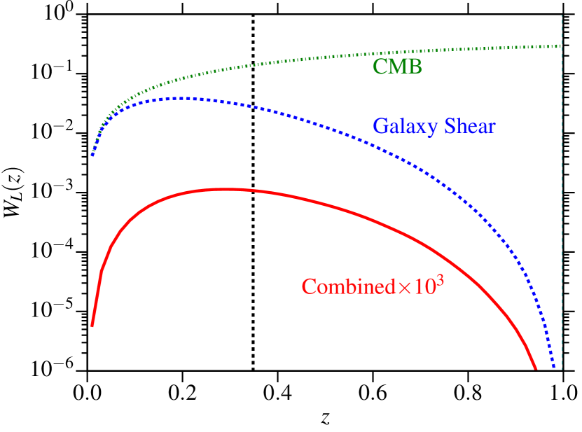
The CMB lensing weight (or kernel) decreases sharply at low redshift, while the galaxy lensing weights depends on the redshift distribution of source galaxies. In Fig. 1 we show the redshift-dependent weights of both CMB lensing and galaxy lensing (calculated using the SDSS source sample redshift distribution as described in Sec. 3.3) as a function of redshift, as well as the combined weight given by
| (12) |
for CMB and galaxy shear are defined in Eq. (11); , the growth function normalized to 1 at , accounts for the growth of matter perturbations with redshifts. In this work, we will use source galaxies with photometric redshift values satisfying (see section 3.3). The galaxy lensing weight peaks around and the combined weight peaks around , though it is skewed towards higher redshift with .
2.3 Lensing signal around galaxies
When studying the lensing signal around galaxies, we are interested in measuring the projected average surface mass density around the lens galaxy sample. We start by writing the convergence and shear as
| (13) | |||
| (14) |
is the mean projected surface mass density within the radius (transverse comoving), and the critical surface density is defined in comoving coordinates as
| (15) |
The factor is required to convert the factor to comoving space since it has dimensions of . We can write in terms of the projected surface mass density as
| (16) |
where is the line of sight distance from the galaxy in redshift space, and is the three dimensional galaxy-matter cross-correlation function. Here we use rather than since the shear is only sensitive to the matter density contrast, i.e., , where is the background projected surface mass density. Throughout this paper when using , we mean . The projected matter-galaxy correlation function can be derived from matter power spectrum as
| (17) |
where is the linear galaxy bias and is the galaxy-matter cross-correlation coefficient, assumed here to be independent of redshift. The linear bias assumption is only valid at linear scales , and at smaller scales there are substantial contributions from non-linear bias (Baldauf et al., 2010; Mandelbaum et al., 2013). In this work we primarily use scales where the linear bias model is valid, and analysis with a scale-dependent bias will be presented in future work. To first order, lensing measurements are not affected by redshift space distortions and hence we do not include any corrections for that. The weight function depends on the redshift distribution of source galaxies and on any redshift-dependent weights used when estimating the signal (see Sec. 2.5). We explicitly calculate these weights and include them in the theory calculations, which integrates over the whole redshift range while using the weights (but does assume redshift-independent and ). For a nearly volume-limited sample like LOWZ, this is a quite good assumption, but in general if the bias and do evolve with redshift, we will measure an effective value averaged over redshift.
2.3.1 1-halo term: Galaxy-galaxy lensing
To model the small-scale signal (), we use the NFW profile (Navarro et al., 1996), for which the 3D density is
| (18) |
The NFW profile can be integrated over the line-of-sight to get the projected mass density, and then
| (19) | |||
| (20) |
For NFW profiles, we define the concentration, , and mass, , using a spherical overdensity of times the mean density:
| (21) |
We use the colossus111http://www.benediktdiemer.com/code/ software (Diemer & Kravtsov, 2015) to compute the NFW profiles with the mass-concentration relation from Bhattacharya et al. (2013). To avoid the contamination from the host halo (for those galaxies that are satellites within some larger host halo) and halo-halo terms, we fit the NFW profile only in the range in case of galaxy-galaxy lensing.
2.3.2 1-halo term: Galaxy-CMB lensing
In the case of CMB lensing, as described in Sec. 3.4, the Planck CMB lensing maps only go up to , which corresponds to a hard edge in that effectively smoothes out the configuration-space maps at scales. To model the signal, we then have to smooth out the NFW profile by convolving it with a sinc kernel () and with a tophat kernel with size set by the resolution of the healpix map being used. However, is the virial radius at all redshifts and expected halo masses of our samples, and thus the measured profiles on all scales will have contributions from satellite and halo-halo terms. Since the simple NFW profile does not contain these contributions, mass estimates using only the NFW profiles will be biased high. To get more correct mass estimates, one should use a halo model. However, since the signal-to-noise ratio of the CMB lensing at these scales is fairly low, and there are additional uncertainties in the measurement from the Planck beam and possible leakage of foregrounds and astrophysical systematics such the thermal SZ effect (van Engelen et al., 2014), we do not attempt more complicated modeling in this work. Instead, for a qualitative comparison, we will present convolved profiles by defining and as
| (22) |
| (23) |
where is measured directly from the data as described in Sec. 2.4 and 2.5.4. At very small scales, the measurement is likely to be biased because of imperfect corrections for fiber collisions (see Sec. 3.2). Hence we down-weight at these scales and use the NFW profile, which should provide an adequate estimates for the small-scale profile. We fit this profile to the data with the NFW halo mass as a free parameter. However, these mass constraints could be biased because of several approximations being made in this model, so they too should be taken as a rough guide.
Finally, we will also present a comparison with measured from the ‘Med-Res’ -body simulations that were first presented in Reid et al. (2014), using the and snapshots for LOWZ and CMASS galaxies, respectively. The sample of halos we use is generated using an HOD model from Zheng et al. (2005) fit to the clustering of galaxies assuming fixed abundance of parent halos of the galaxies, with priors on abundance being derived from range of redshift-dependent abundance of galaxies (see Reid et al., 2014, for more details). To get , we cross-correlate the halos with matter particles to obtain , which is then multiplied with to get .
We note that the smoothing kernel is only applied to the theoretical predictions when fitting a model to the small-scale signals below the resolution of the Planck convergence maps. When fitting large scales (), we have confirmed that the effects of smoothing are negligible, and hence we do not apply the smoothing kernel to the theoretical predictions in those cases.
2.4 Galaxy Clustering
We also measure the two-point correlation function of galaxies to constrain their large-scale (linear) bias. In the linear bias regime, the two-point correlation function of galaxies is given by
| (24) | ||||
| (25) |
The Kaiser factor, , accounts for the redshift space distortions in the linear regime (Kaiser, 1987), where , is the linear growth rate factor at redshift and . The weight function is given by Mandelbaum et al. (2011) as
| (26) |
Here is the redshift probability distribution for the galaxy sample.
Finally we integrate over the line-of-sight separation to get the projected correlation function
| (27) |
We use to reduce the effects of redshift space distortions (van den Bosch et al., 2013).
2.5 Estimators
In this section we present the estimators used for measuring various signals. For all measurements, we use 100 approximately equal-area ( on a side) jackknife regions to obtain the jackknife mean and errors for each bin, as described in Singh et al. (2015) in more detail. When fitting measurements to theoretical predictions, we use a weighted least squares method to fit each jackknife region using just the diagonal elements of jackknife covariance matrix, and then quote the jackknife mean and errors on the best-fitting parameters. When doing MCMC fits (Sec. 4.3), we use the jackknife covariance matrix.
2.5.1 Galaxy-Galaxy Lensing
For galaxy-galaxy lensing we measure as
| (28) |
The summation is over all lens-sources (ls) pairs, where the weight for each lens-source pair is defined as (see e.g. Singh et al., 2015, for more detail)
| (29) |
is the shape noise and is the measurement noise for the source galaxy. The enters the weight because we defined the in Eq. (28) as the maximum-likelihood estimator (Sheldon et al., 2004). Note that the denominator in the first term in Eq. (28) has a weight , measured by using random lenses rather than real lenses. This accounts for the dilution of the shear by unsheared “source” galaxies that are actually associated with the lens but are put behind the lens due to photometric redshift scatter. The correction factor for this effect, , is usually called the boost factor (Sheldon et al., 2004; Mandelbaum et al., 2005). Finally, the second term in Eq. (28) is the subtraction of the measured around the random lenses, to remove the effect of spurious shear at large scales (Mandelbaum et al., 2005).
To measure only the tangential shear around galaxies, we use the estimator
| (30) |
where the weight for galaxy-galaxy lensing (but not cosmography; see Sec. 2.7) is defined as
| (31) |
2.5.2 Cross-correlation between galaxy positions and CMB convergence
CMB lensing measurements provide convergence measurements on the sky, with the sky being divided
into equal area pixels using healpix222http://healpix.sf.net/
https://github.com/healpy/healpy (Górski
et al., 2005).
Using these measurements, we can obtain the projected surface mass density
around lens galaxies as
| (32) |
where the summation is carried over all lens galaxy-CMB pixel pairs () separated by comoving projected distance at the lens redshift, where and define the bin edges. is the geometric factor defined in Eq. (15) with CMB as the source. The weight factor is defined as
| (33) |
We do not include pixel noise in the weights since each pixel has the same statistical noise. Finally we subtract out the signal measured around random galaxies ( pairs), to remove the spurious signal from noise (more discussion in section 4.1).
To measure the convergence signal around galaxies, we use the estimator
| (34) |
The rationale for and effect of subtracting the mean convergence around random points is discussed in Sec. 4.1. Under the assumption that each pixel has the same statistical noise, we adopt uniform weights: .
2.5.3 Cross-correlation between galaxy shear and CMB convergence
For lensing-lensing cross-correlations, we measure the tangential shear around the pixels of the CMB map and multiply it with the CMB convergence measured in that pixel.
| (35) |
The summation is over all pixel () and source galaxy () pairs with separation , where and define the bin edges. The weights are inverse variance weights for source galaxies, accounting for shape noise and measurement noise.
| (36) |
2.5.4 Galaxy Clustering
We use the Landy-Szalay (Landy & Szalay, 1993) estimator to compute the two-point correlation function:
| (37) |
is the count of galaxy-galaxy pairs, is count of galaxy-random pairs and are the random- random pairs. The projected correlation function is obtained by integrating over the line-of-sight separation () bins
| (38) |
We use , with 20 line-of-sight bins of size . The choice of bin size does not significantly impact our results since the redshift extent of our sample is . The choice of also does not affect our measurements; measurements with are not signifcantly different from . We do use the correct in our theory predictions to account for redshift-space distortion effects.
2.6 Removing small-scale information
When measuring galaxy-galaxy lensing for which the observable is , information from the matter distribution on small scales affects the signal measured at large scales as well. If we have a valid model for correlation functions on all scales, this is not a problem. However, perturbation theory-based methods cannot model signals within the virial radius of virialized halos, and even at somewhat larger scales (), lowest order perturbation theory is not valid. To some extent this problem can be alleviated by using non-linear prescriptions that describe quasi-linear scales with some success. Baldauf et al. (2010) suggested an approach for removing the small-scale information by defining a new estimator
| (39) |
and () can also be converted to using the relations between and both in the data and theory. Baldauf et al. (2010) showed that using not only removes small-scale information that is difficult to robustly model, it also reduces the impact of cosmic variance and redshift-space distortions in the projected correlation functions. The trade-off made when using is that we are removing signal when computing , so the signal-to-noise ratio () in the measurements decreases, especially at scales near . Thus we want to choose lower to use more signal and have higher , and higher to be able to remove non-linear galaxy bias more effectively. Baldauf et al. (2010) suggests using , where is the virial radius of haloes in the sample. For BOSS LOWZ galaxies, and hence we will use or greater in our analysis. As stated, using helps in reducing the impact of cosmic variance, which improves the , particularly on large scales and at least partially compensates for the lost at small scales.
We will use to derive most of the constraints on galaxy bias , galaxy lensing amplitude, and the galaxy-matter cross-correlation coefficient . In principle, for the combination of CMB lensing and galaxy clustering, using is unnecessary since the observables at a given are not contaminated by information from smaller . However, use of a consistent estimator for all probes is valuable. Moreover, while use of reduces the to some extent (this is dominated by reduced at small scales, as we will show explicitly in Fig. 9), the is moderately improved on the large scales that dominate our constraints.
2.7 Cosmography
Hu et al. (2007b) proposed the idea of using the ratio of CMB convergence and galaxy lensing convergence as a way to measure the distance ratio (distance to surface of last scattering relative to the distance to the source galaxy sample used to estimate the galaxy lensing) and hence constrain the geometry, and the equation of state of dark energy. The ratio is defined as
| (40) |
Similar distance ratio tests have also been proposed using galaxy or galaxy cluster lensing alone, in both strong lensing (eg. Link & Pierce, 1998; Golse et al., 2002) and weak lensing regimes (eg. Jain & Taylor, 2003; Bernstein & Jain, 2004). Several studies have already measured the distance ratios (e.g. Taylor et al., 2012; Diego et al., 2015; Kitching et al., 2015; Caminha et al., 2016, and references therein), though they are afflicted by several systematics such uncertainties in modeling cluster profiles and cosmic variance in case of multiple strong lens systems, and photometric redshift uncertainties as well as imaging systematics that cause a redshift-dependent shear calibration in the case of weak lensing. The small redshift baseline also limits the cosmological applications of these measurements using optical weak lensing alone (see discussion in Hu et al., 2007b; Weinberg et al., 2013). Using CMB lensing in cosmographic measurements is advantageous in several ways. First, the source redshift for the CMB (redshift of surface of last scattering) is well known, so one of the two redshift slices being compared has no redshift uncertainty. The long redshift baseline between CMB and galaxy lensing sources also improves the sensitivity of to cosmological parameters (Hu et al., 2007b). However, using CMB lensing with galaxy lensing makes become more sensitive to some of the systematics in galaxy lensing (for example, multiplicative bias) and can also be used as test for presence of such systematics.
To measure , we work with galaxy lensing shear measured using estimator defined in eq. (30), not convergence. Instead we convert the convergence measurement from CMB (measured using estimator defined in eq. (34)) to the shear. Motivated by the estimator in Sec. 2.6, we define the estimator as
| (41) |
Just as , we can write . In the limit that , is simply . The CMB lensing convergence averaged around lens galaxy positions can be converted to using and then converting to .
One of the primary motivations for defining was to remove information for small scales which are more difficult to model. When measuring , we do not need to model those small scales (any nonlinear bias, etc. will cancel in the ratio) and hence using is not strictly necessary. However, when computing the convergence signal from the CMB, the smallest scales are smoothed (see Sec. 3.4) and it is desirable to completely remove information from those scales. Thus we will use to compute and our final definition of the estimator is
| (42) |
Note that our estimator is different from the one used by Miyatake et al. (2016), who use to compute and exclude the scales which are affected by smoothing. We will show our measurement using small value of ( smoothing scale), in which case our estimator is equivalent to one using and excluding scales smaller than smoothing scale. Also in the estimator of Miyatake et al. (2016), the galaxy-galaxy lensing measurement is in the numerator, so their estimator is effectively . We keep the CMB lensing measurement in the numerator since it is noisier. Later in this section we describe how we account for the bias that comes from taking the expectation value of the ratio of noisy quantities.
To model the measurement, we begin by computing the galaxy position-convergence and galaxy position-shear cross-correlations
| (43) | ||||
| (44) |
where source weights are defined in Sec. 2.5.1 The theory computations can be converted to using similar method as in the data. Note that due to variations in the number density of source galaxies, galaxy-CMB and galaxy-source cross correlations measurement are at different effective lens redshifts. In principle this can be modeled, but a desirable feature in is to define it as a simple ratio without requiring complicated modeling for small scale signals. To get both signals at the same effective redshift, we explicitly compute the weights from galaxy-galaxy lensing as a function of lens redshift, and use them as weights when computing the galaxy-CMB lensing cross-correlations. These weights decrease strongly with redshift due to the decrease in the number of source galaxies behind a lens for increasing lens redshift. Since CMB lensing kernel increases with redshift, these weights are suboptimal for galaxy-CMB lensing cross correlations and increase the noise in measurements. Since the measurement is noisier and dominates the noise in , it is desirable to modify the weights to give higher weight to higher redshift galaxies. Thus we add an additional factor of to weights. This increases the noise in the measurement from galaxy-galaxy lensing, but this increase is more than balanced by the reduced noise in from galaxy-CMB lensing cross correlations. The final lens weights are defined as
| (45) |
Finally is given as
| (46) |
is the matter growth function and enters because scales as in linear theory. In principle, due to non-linear effects in , the weights in can vary with the scale. Since non-linear effects also evolve with redshift, the measurement of at different scales can be at somewhat different effective lens redshifts, , and hence can in principle be scale-dependent. However, this effect is likely to be small given the narrow redshift range of LOWZ sample, and should be subdominant to the noise in our measurements. When comparing with data, we show this effect by replacing with scale dependent growth function () estimated from correlation function using linear theory with halofit nonlinear evolution. We do note that halofit does not capture the full non-linear evolution at small scales and thus our estimate will only be approximate.
To estimate the bias that comes from taking the ratio of noisy quantities before taking the expectation value, we make mock realizations of the numerator and denominator in Eq. (46), using the signal-to-noise ratio from CMB measurements for numerator and galaxy lensing measurements for the denominator.
| (47) |
where is either the numerator or denominator and is measured from CMB (galaxy) lensing for numerator (denominator). Using , we generate random realizations, assuming gaussian distribution with mean and standard deviation . We then recompute the taking the ratio of and then compute the mean, , using the same scales as . We include the bias estimated from this exercise in the theory prediction before comparing with the data.
3 Data
3.1 SDSS
The SDSS (York et al., 2000) imaged roughly steradians of the sky, and the SDSS-I and II surveys followed up approximately one million of the detected objects spectroscopically (Eisenstein et al., 2001; Richards et al., 2002; Strauss et al., 2002). The imaging was carried out by drift-scanning the sky in photometric conditions (Hogg et al., 2001; Ivezić et al., 2004), in five bands () (Fukugita et al., 1996; Smith et al., 2002) using a specially-designed wide-field camera (Gunn et al., 1998) on the SDSS Telescope (Gunn et al., 2006). These imaging data were used to create the catalogues of shear estimates that we use in this paper. All of the data were processed by completely automated pipelines that detect and measure photometric properties of objects, and astrometrically calibrate the data (Lupton et al., 2001; Pier et al., 2003; Tucker et al., 2006). The SDSS-I/II imaging surveys were completed with a seventh data release (Abazajian et al., 2009), though this work will rely as well on an improved data reduction pipeline that was part of the eighth data release, from SDSS-III (Aihara et al., 2011); and an improved photometric calibration (‘ubercalibration’, Padmanabhan et al., 2008).
3.2 SDSS-III BOSS
Based on the photometric catalog, galaxies were selected for spectroscopic observation (Dawson et al., 2013), and the BOSS spectroscopic survey was performed (Ahn et al., 2012) using the BOSS spectrographs (Smee et al., 2013). Targets are assigned to tiles of diameter using an adaptive tiling algorithm (Blanton et al., 2003), and the data were processed by an automated spectral classification, redshift determination, and parameter measurement pipeline (Bolton et al., 2012). In this paper we use the BOSS data release 12 galaxies (Alam et al., 2015).
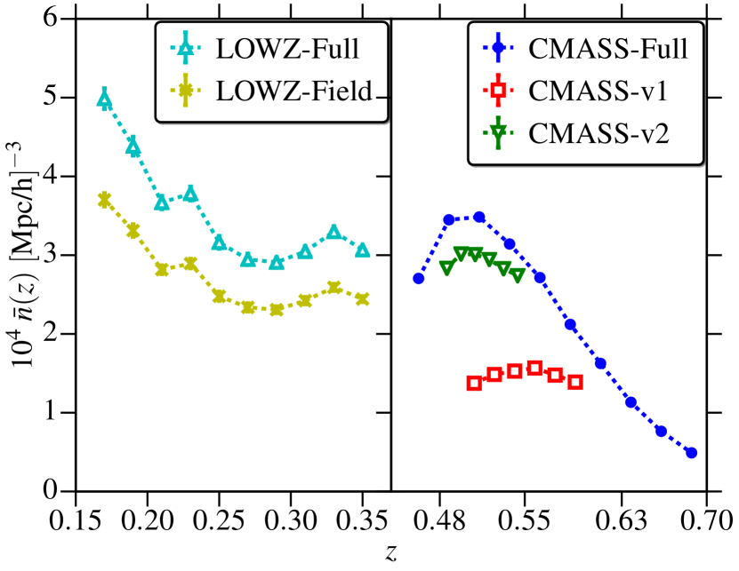
The number densities of the BOSS samples and of various subsamples used in this work are shown in Fig. 2.
3.2.1 LOWZ
The LOWZ sample consists of Luminous Red Galaxies (LRGs) at , selected from the SDSS DR8 imaging data and observed spectroscopically in the BOSS survey (Reid et al., 2016). The sample is approximately volume-limited in the redshift range , with a number density of (Manera et al., 2015; Reid et al., 2016). BOSS DR12 has 249 938 LOWZ galaxies within the redshift range used in this work, . After combining with the Planck lensing map mask and the SDSS shape catalog mask, which masks out certain regions that have higher Galactic extinction or poor imaging quality (Reyes et al., 2012), we are left with 225 181 LOWZ galaxies, with redshift-dependent number density shown in Fig. 2.
We also define a sample of field galaxies using the Counts in Cylinders methods (Reid & Spergel, 2009), which was used in Singh et al. (2015) to define a sample of groups from LOWZ galaxies. Here we apply the same technique to DR12, and select field galaxies by requiring that they are in groups of one galaxy and that their fiber collision and redshift failure weights are equal to 1 (see Sec. 3.2.3). These cuts ensure that there is no neighboring target LOWZ galaxy within and for the field galaxies. Field galaxies by construction have no redshift failure weights (see Sec. 3.2.3) and thus will provide a test on any possible systematics from these weights. They also tend to reside in lower mass halos, and are less likely to be satellites (which have lensing profiles that are more complex to interpret on small scales due to contamination from the host halo lensing profile).
3.2.2 CMASS
The BOSS CMASS sample consists of higher redshift galaxies () targeted using color and magnitude cuts intended to select a uniform sample of massive galaxies (Reid et al., 2016). The DR12 CMASS sample has 849 637 galaxies, of which we use 682 298 after applying the masks and a redshift cut . The number density of the CMASS sample varies across the redshift range (see Fig. 2), which can bias the inferences of its properties from stacked galaxy position-lensing cross correlations. To overcome this problem, we also define two volume-limited samples: CMASS-v1, with and , and CMASS-v2, with and , where is the absolute magnitude corrected to using method described in Wake et al. (2006). CMASS-v1 has 188 586 galaxies with , where denotes the maximum variation across the redshift range. CMASS-v2 has 236 676 galaxies with . Since both volume-limited samples have a narrow redshift range, we use when calculating the clustering signal for these samples.
3.2.3 Weights
In their large scale structure (LSS) samples the BOSS collaboration provides several weights for each galaxy to correct for systematics when estimating the galaxy clustering(Reid et al., 2016). The most important of these are the fiber collision and incompleteness (redshift failure) weights. Due to the finite size of the spectroscopic fibers, it is impossible to simultaneously take spectra of BOSS galaxies that are separated by less than . Many of these cases are resolved by revisiting the field multiple times. However, some target galaxies lack spectroscopic redshifts either due to fiber collisions and redshift failures. This introduces a bias in the clustering measurements, since the fiber-collided galaxies are preferentially located in overdense regions. An approach that has been shown to work on large scales () (Reid et al., 2014) is to upweight the nearest neighbor of the fiber-collided galaxies, based on the assumption that they are likely to be in the same group due to their proximity on the sky.
In addition, we also use systematics weights, which correct for the effects of varying target density as a function of stellar density for the CMASS sample (Ross et al., 2012) The final weights used for CMASS are
| (48) |
where corrects for fiber collisions, and for LOWZ. While these weights have been shown to correct for biases in clustering on large scales, it is not clear whether this approach works well for lensing calculations (see More et al., 2015). is not expected to change the lensing measurements done by stacking procedure, as long as these weights do not alter the overall properties of the sample. These systematic weights do depend on the apparent surface brightness of the galaxies, as those with low surface brightness are more likely to be missed in regions of high stellar density (Ross et al., 2012). However, the dependence on surface brightness is sufficiently mild that their inclusion does not significantly alter the properties of the sample. We checked that using these weights changes the absolute magnitude and redshift distribution of the sample by and thus we do not expect any significant changes in the lensing measurement from . Still, we do use these weights for all samples and subsamples of CMASS. Redshift failure weights do change both the lensing and clustering measurements by up-weighting the higher density regions. However, they do not mitigate the bias below the fiber collision scale, and even at slightly larger scales, the measurements will be biased since we are stacking on the wrong galaxy. Still, at scales , these weights should not lead to any significant change other than changing the effective galaxy bias . In Appendix A, we directly show the effect of using these weights using the CMASS sample. For field galaxies, these weights are all equal to one and for volume limited sub-samples of CMASS, it is not guaranteed whether the galaxies missed from redshift failures will pass the magnitude cuts. Hence we omit the results using redshift failure weights for these sub-samples.
3.3 SDSS shear catalog
For galaxy-galaxy lensing (shear measurements), we use the SDSS re-Gaussianization shape catalog that was introduced in Reyes et al. (2012). Briefly, these shapes are measured using the re-Gaussianization algorithm (Hirata & Seljak, 2003). The algorithm is a modified version of early ones that used “adaptive moments” (equivalent to fitting the light intensity profile to an elliptical Gaussian), determining shapes of the PSF-convolved galaxy image based on adaptive moments and then correcting the resulting shapes based on adaptive moments of the PSF. The re-Gaussianization method involves additional steps to correct for non-Gaussianity of both the PSF and the galaxy surface brightness profiles (Hirata & Seljak, 2003). The components of the PSF-corrected distortion are defined as
| (49) |
where is the galaxy minor-to-major axis ratio and is the position angle of the major axis on the sky with respect to the RA-Dec coordinate system. The ensemble average of the distortion is related to the shear as
| (50) | ||||
| (51) |
where is the per-component measurement uncertainty of the galaxy distortion, and is the shear responsivity representing the response of an ensemble of galaxies with some intrinsic distribution of distortion values to a small shear (Bernstein & Jarvis, 2002).
For this sample, we use photometric redshifts derived from the template fitting code ZEBRA (Feldmann et al., 2006), as described and characterized in Nakajima et al. (2012). Using photometric redshifts can also introduce bias in galaxy-galaxy lensing measurements. Nakajima et al. (2012) showed that this bias can be large, but can be determined to percent accuracy using representative spectroscopic calibration samples. Using the calibration method described in Nakajima et al. (2012), we estimate the calibration bias for the galaxy-galaxy lensing by the LOWZ sample to be , and thus multiply our lensing signal by a factor of 1.1 before plotting it or fitting models to it.
When estimating the galaxy lensing-CMB lensing cross-correlations, we do not need redshifts for individual source galaxies. To derive the theoretical predictions for this quantity, we directly use the obtained from the representative spectroscopic redshift dataset from Nakajima et al. (2012) after applying the same cuts that were applied to data during measurements.
3.4 Planck Lensing Maps
We use the Planck 2015 lensing map provided by the Planck collaboration (Planck Collaboration et al., 2015a). We convert the provided values to a convergence map using healpy (Górski et al., 2005), with n (pixel size of ), where n determines the resolution of the healpy map (higher n means smaller pixels; over the full sky). When constructing the convergence map, we use in the range , which corresponds to modes from to . Planck Collaboration et al. (2015a) found some evidence of systematics in the high range, and used (‘conservative’) for their main cosmological constraints, though using the ‘aggressive’ range that is adopted here gives a very similar amplitude of the lensing power spectrum and constraints for cosmological parameters except for , which shifts by between the two ranges.
While our primary results use n, we test the effects of changing the pixel size (using n and 2048, with pixel sizes of and respectively) and applying smoothing on the convergence maps (Gaussian beams with and ). Since the pixel size with n is somewhat greater than the smoothing scale in the lensing map, we do expect to gain some information by using smaller pixels with n. Going to even higher resolution with n should not make a very significant difference except at very small scales, in case there is some information left in the lensing maps at those scales. Similarly, smoothing with a Gaussian beam with should not significantly affect our results given the resolution of the Planck maps and the scales used for our measurements, though should change the signal on scales up to the FWHM () of the smoothing kernel. Hence we will omit the measurements with and will show results with smoothing for comparison with the main results, which have no additional smoothing applied to maps.
When calculating the cross-correlations, we apply the common galaxy and Planck mask on both the galaxy shear and Planck convergence maps. This reduces the area within the BOSS mask by , primarily driven by the Planck point source mask which selectively masks the very massive clusters. This can change the effective linear bias of the galaxy samples and hence we use the same mask when computing galaxy clustering as well as galaxy-galaxy lensing.
To perform null tests, we generate a map by shuffling the pixels in the convergence map (with the Planck mask applied) and then applying the galaxy mask. We also generate a realization of a noise map using the noise power spectrum provided with the lensing maps. Throughout this work, and will be used to represent the shuffled map and noise map convergences, respectively.
4 Results
4.1 Lensing of the CMB by galaxies
In this section we present the results from cross-correlating the Planck convergence maps with the lens galaxy samples described in Sec. 3.2.
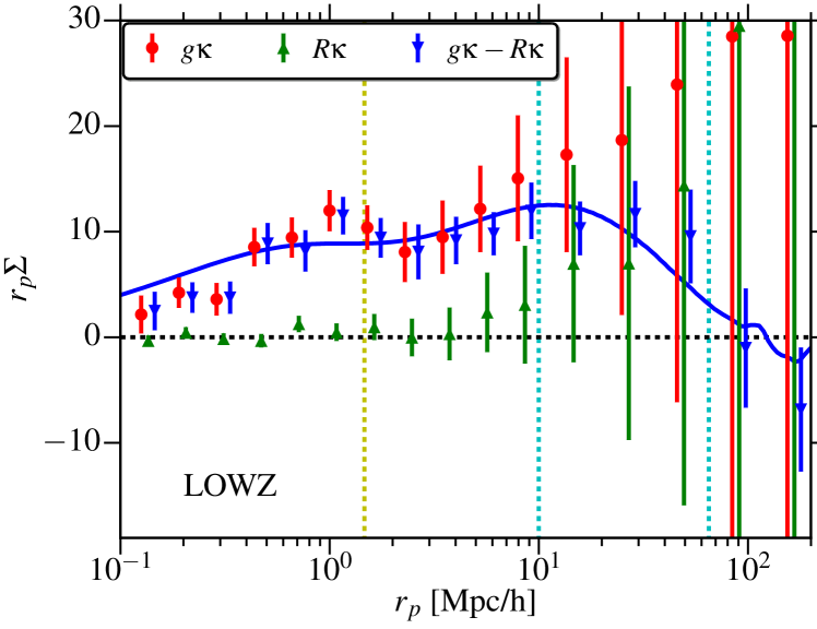
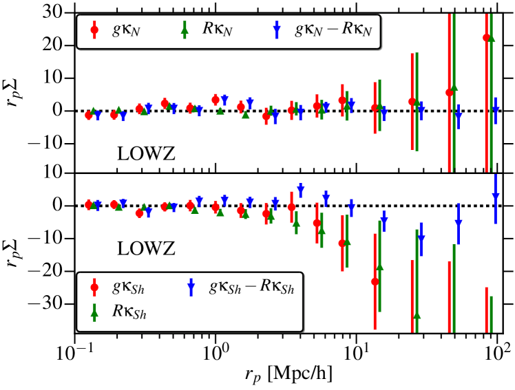
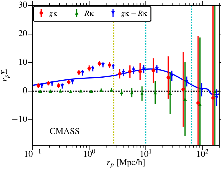
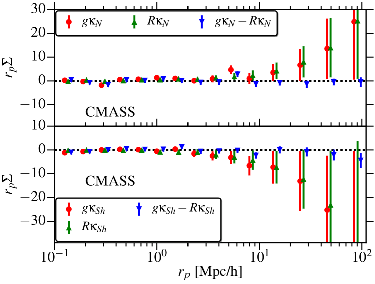
Figure 3 shows the cross-correlation signal for galaxy position vs. CMB lensing for both the LOWZ and CMASS samples. We show the signal measured around the galaxies and around random points. At small scales, there is significant signal around galaxies, and the the measurements in different bins are uncorrelated. At large scales, the lower signal and the fact that the stack in each bin includes almost all pixels in the map leads to the signal being dominated by the noise in the CMB convergence, and hence the bins are very strongly correlated (we are effectively measuring the mean and standard deviation of the map in every bin). This noise can be removed by subtracting out the signal measured around random points from the signal measured around the galaxies, as shown in Eq. (32). Another way to understand the effect of this random subtraction is that similar to the Landy-Szalay estimator in clustering, we want to correlate the CMB map with a mean zero quantity (), so that any additive systematics are removed to first order (Mandelbaum et al., 2006). After subtracting, the different bins exhibit less substantial but still noticeable correlations even at large scales, as shown in Fig. 5.
The final measurements after subtracting the signal around random points are consistent with the Planck 2015 CDM model predictions. The solid lines in Fig. 3 show the linear theory halofit correlation functions with the best-fitting galaxy bias, ; the parameters of these fits are presented in Table 1. We only fit this model for scales , as at smaller scales, the effects of non-linear bias and stochasticity in the galaxy-matter cross-correlation are expected to cause deviations between the data and the model. However, as shown in Fig. 3, there is no evidence of tension between the theory and the data even down to . On the scales used for the fits, for LOWZ (CMASS). Given the large minimum radius for the fits, the constraints on galaxy bias are independent of the pixel size and of the smoothing imposed by the cutoff in the CMB map at . We remind the reader that the minimum radius for the fits is larger than the resolution of the convergence maps, and hence the results from fitting to theoretical models in this section do not have any smoothing applied to the models. We will discuss the small scale signal, where smoothing is necessary, in Sec. 4.2.
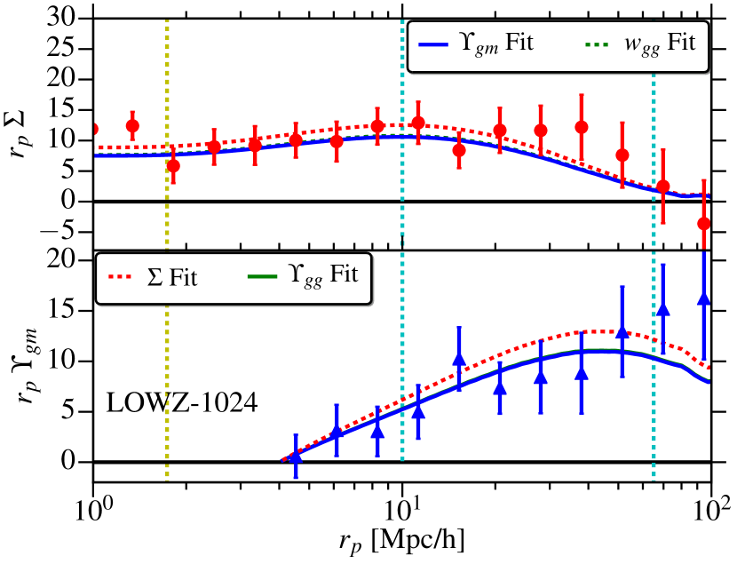
In Fig. 4 we show the comparison of and with the predictions from Planck theory model using the best fitting bias from , , and . As shown in Fig. 4 and Table 1, there is some discrepancy between the obtained from and . These discrepancies are not very significant ( after accounting for correlations). This is mostly caused by the noise in the measurements, which leads to mild tension between theory and data as they have slightly different scale dependences. Differences in the scale dependence of the theory and data can in general lead to different bias measurements from and , since at any scale depends on values at scales smaller than (but greater than ).
| Lens sample | Pixel | ||||
|---|---|---|---|---|---|
| size | |||||
| LOWZ | 6.9′ | 1.800.30 | 2.200.50 | 13.56.5 | |
| LOWZ | 3.4′ | 1.800.28 | 2.120.46 | 13.93.9 | |
| LOWZ | 3.4′ | 1.870.27 | 2.200.40 | 17.17.4 | |
| LOWZ | 1.7′ | 1.750.28 | 2.210.46 | 11.83.6 | |
| LOWZ | |||||
| Field | 3.4′ | 1.610.26 | 1.900.40 | 13.53.9 | |
| Field | |||||
| CMASS | 6.9′ | 1.500.20 | 1.460.28 | 24.95.7 | |
| CMASS | 3.4′ | 1.750.15 | 1.600.20 | 34.36.4 | |
| CMASS | 1.7′ | 1.560.19 | 1.510.27 | 6.92.3 | |
| CMASS-v1 | 3.4′ | 1.640.29 | 1.800.40 | 45 | |
| CMASS-v2 | 3.4′ | 1.530.29 | 1.310.39 | 16.34.5 |
The right column of Fig. 3 also shows the null tests for these measurements. The signal around random points is consistent with zero at all scales, though the noise at large scales is dominated by the reconstruction noise in CMB lensing. When using the shuffled CMB lensing map, the signal around random points, galaxies, and their difference is consistent with zero. Finally, the signal measured using the noise map is also consistent with zero. The noise map also serves as a diagnostic for our covariance estimates as shown in Fig. 5, since it has the same correlated noise properties. The Jackknife covariance and correlation matrices obtained from measurements using the CMB map and noise map are consistent. In Appendix B we show the consistency between the jackknife covariance matrix and the covariance matrix obtained using 100 independent realizations of the noise maps.
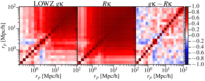
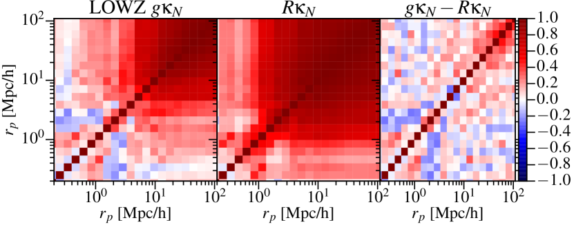
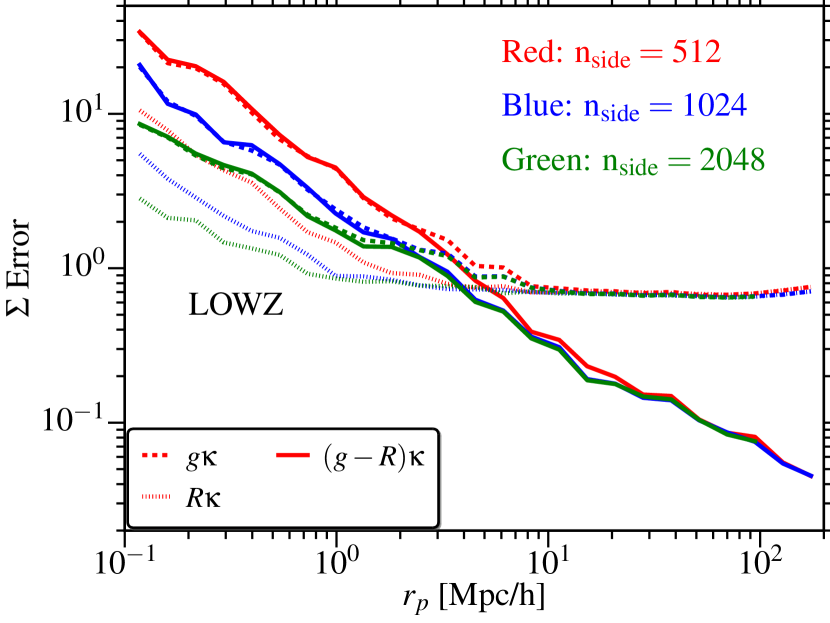
Fig. 6 shows the scaling of the errors with , and a comparison of errors using different pixel sizes for LOWZ; CMASS results, which are not shown, are similar. Going to smaller pixel size improves the signal-to-noise ratio at small scales, which suggests that there is some information available at these scales In Fig. 6, we show results for n, 1024 and 2048. Using n results in some improvement at small scales, but the results are comparable to those with n at scales , motivating our choice of n for our primary results. However, our galaxy bias constraints that are based on large scales are not significantly affected by the choice of n.
Also in Fig. 6, statistical uncertainties on the signals around galaxies and random points saturate for scales (). This saturation results from the fact that once we have stacked many pixels, we are limited by the reconstruction noise of the CMB lensing maps. This noise is also the reason for the strong bin-to-bin correlations in the first two columns in Fig. 5. After subtracting the signal around random points, the final signal is still dominated by noise in the CMB convergence measurements, but there is no evidence of residual systematics from our null tests. Moreover, Fig. 5 shows that there are only mild to moderate correlations between the bins.
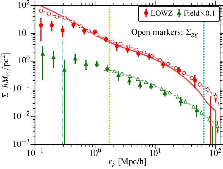
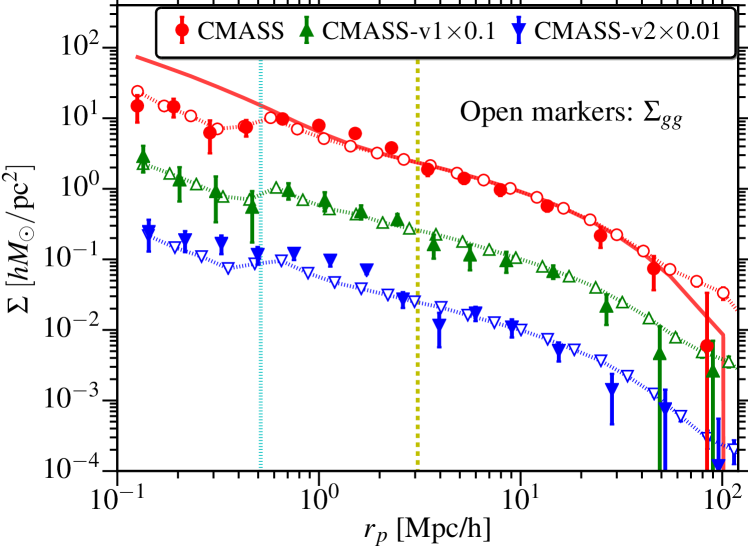
In Figure 7, we show the measured using CMB lensing from Fig. 3 with the measured from simulations and the clustering measurement by converting the clustering into using Eq. (22), where we use the best fit to the clustering signal. The signals are consistent at most scales, though the comparison with clustering is only qualitatively valid. At small scales, the effects of non-linear galaxy bias and the stochasticity in the galaxy-matter cross-correlation can lead to differences between the two. Also, in the BOSS data, the clustering below is affected by the incompleteness due to fiber collisions, which biases the signal for in the case of LOWZ (CMASS) sample, even when weights are used (even with weights, clustering is not unbiased for ). The lensing signal is also affected since fiber collisions preferentially affect the higher density regions which lead them to be under-weighted in the lensing measurements as well. While fiber collision weights do attempt to correct the bias, the signal is still biased at small scales since we are stacking on the wrong galaxies. The CMB lensing measurement at these scales is also affected by the pixel size and smoothing of the Planck maps. At large scales, the clustering is affected by the residual RSD, while the lensing signal is not to first order. This effect is above . Between , we do expect to find a good agreement () between the CMB lensing and clustering measurements, as demonstrated in Fig. 7.
In Fig. 7, we also show the signals measured for various LOWZ and CMASS subsamples defined in Sec. 3.2. The primary motivation for defining these samples was to test for the effects of redshift failure weights (using field galaxies, which should be less affected by fiber collisions) and variations in number densities with redshift (using volume-limited samples CMASS-v1 and CMASS-v2). We do not find any significant tension in results using the subsamples, with the lensing results being largely consistent with the predictions from theory combined with the bias measurements from clustering.
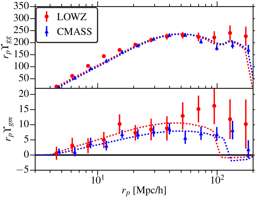
Fig. 8 shows the measurements from the BOSS LOWZ and CMASS samples obtained by converting and measurements into using methods described in Section 2.6 This figure also shows the results from jointly fitting both clustering and lensing measurements with fixed Planck 2015 cosmology to get the galaxy bias and the relative lensing amplitude . Due to the use of weighting in lensing measurements, the clustering and lensing measurements are not at the same effective redshift. As stated in Sec. 2.3, we integrate the theoretical predictions over redshift using the weights, assuming redshift-independent linear bias and . The theory fits the data well within the noise, with and for the CMASS sample and and for the LOWZ sample (see also Table 2). Our measurements are consistent with the theoretical expectation of at linear scales. The galaxy bias measurements for CMASS are consistent with those from Rodríguez-Torres et al. (2016), who measured a scale-dependent bias of –, using scales 10–60. For LOWZ, our bias is consistent with that measured by Singh et al. (2015) using the DR11 sample ().
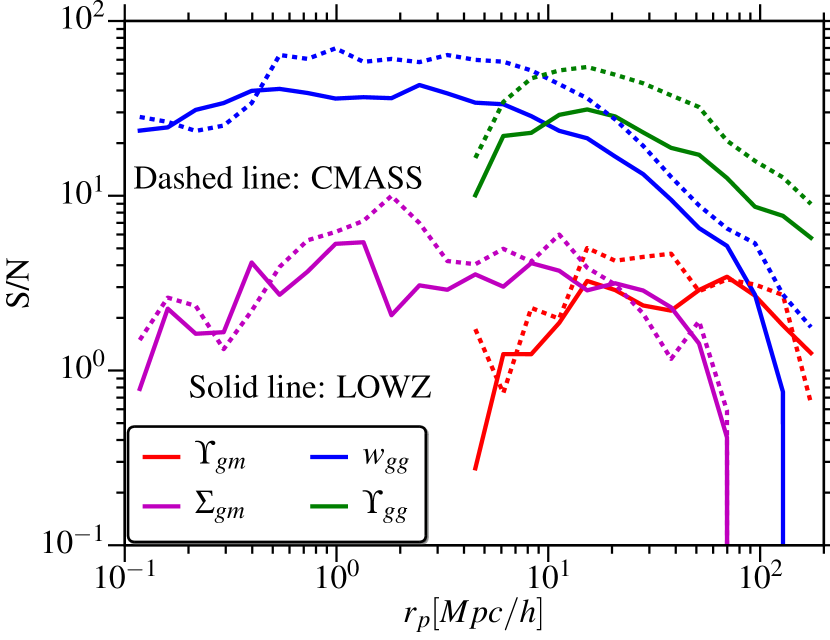
In Fig. 9, we compare the signal-to-noise ratio () for the clustering and CMB lensing measurements using different estimators. has lower signal-to-noise for since by definition it has the signal from scales below removed. However, also reduces the impact of cosmic variance and additive systematics in the measurement, and hence improves the at large scales.
| Sample-Planck | Pix Area | |||
|---|---|---|---|---|
| LOWZ | 3.4′ | 1.750.04 | 1.00.2 | |
| LOWZ | 3.4′ | 1.750.04 | 1.10.2 | |
| CMASS | 3.4′ | 1.950.02 | 0.780.13 | |
| CMASS | 3.4′ | 1.950.02 | 0.80.1 | |
| Field | 3.4′ | 1.470.03 | 1.150.24 | |
| CMASS-v1 | 3.4′ | 2.00.03 | 0.90.2 | |
| CMASS-v2 | 3.4′ | 1.90.03 | 0.70.2 |
4.2 The small-scale signal
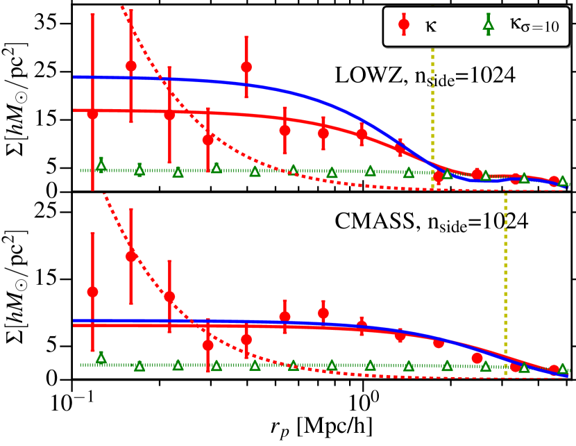
In Figure 7, we show the CMB lensing signal at small separations. As discussed in Sec. 2.3.2 the cutoff effectively smoothens the configuration space convergence map with a two-dimensional sinc kernel. In Fig. 10 we show the measurements only at along with the smoothed profile measured from the simulations (blue lines), described in Sec. 2.3.2. We also show the best-fitting smoothed profile, where the NFW halo mass was set as a free parameter in the fitting procedure. The halo masses are presented in Table 1; these are consistent with the halo mass measured from galaxy-galaxy lensing in the case of the LOWZ and LOWZ-Field subsamples. The halo mass measurement using galaxy-galaxy lensing in this work, , is different from that of Singh et al. (2015), , using BOSS DR11 sample. The difference is primarily driven by the different adopted mass-concentration relations, to which the mass estimates are sensitive when fitting scales as described in Sec. 2.3.1. Using the same mass-concentration relation as Singh et al. (2015), we get consistent results ().
In the case of the LOWZ sample, from simulations over-predicts the signal. This is because the mean halo mass from the simulations is (median mass ), which is higher than the mass preferred by data, , in the case of both the CMB and galaxy lensing measurements.
The halo mass obtained using the fits for the CMASS sample, , is low compared to the values of measured by Miyatake et al. (2015) and Madhavacheril et al. (2015) using galaxy-galaxy and galaxy-CMB lensing respectively. This discrepancy is in the expected direction since tends to over-predict the profile due to the effects of non-linear galaxy bias and hence the NFW mass will be suppressed. Ultimately, the proper interpretation of the lensing signal at small scales requires proper halo modeling, which we do not do given the noise and resolution of Planck CMB lensing maps. Instead we have presented a simple model to enable easy comparisons, but possible biases in this model should be kept in mind. We note that the profile from simulations (after smoothing) is a reasonable description of the data; in the simulated CMASS sample, the mean and median (Reid et al., 2014).
4.3 Lensing calibration: CMB vs. galaxy lensing
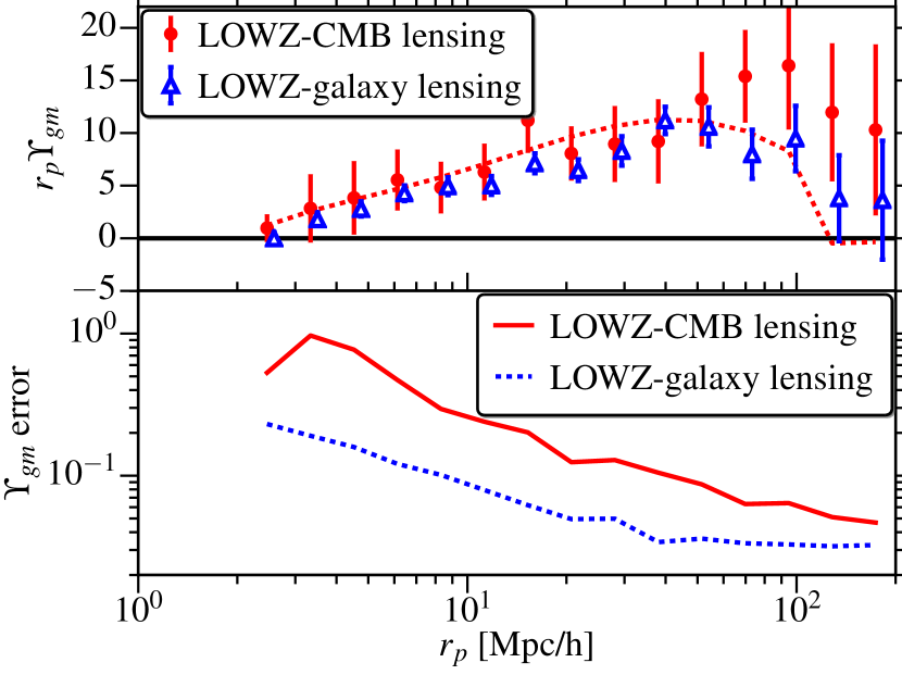
Figure 11 shows the comparison of obtained from galaxy lensing and CMB lensing using LOWZ galaxies as lenses. Note that due to the different weighting used in galaxy lensing and CMB lensing, the two measurements are not at the same effective lens redshift, with () for galaxy (CMB) lensing. In Fig. 11, we also compare the measurement uncertainties, with galaxy lensing having a higher signal-to-noise ratio by a factor of 2–5.
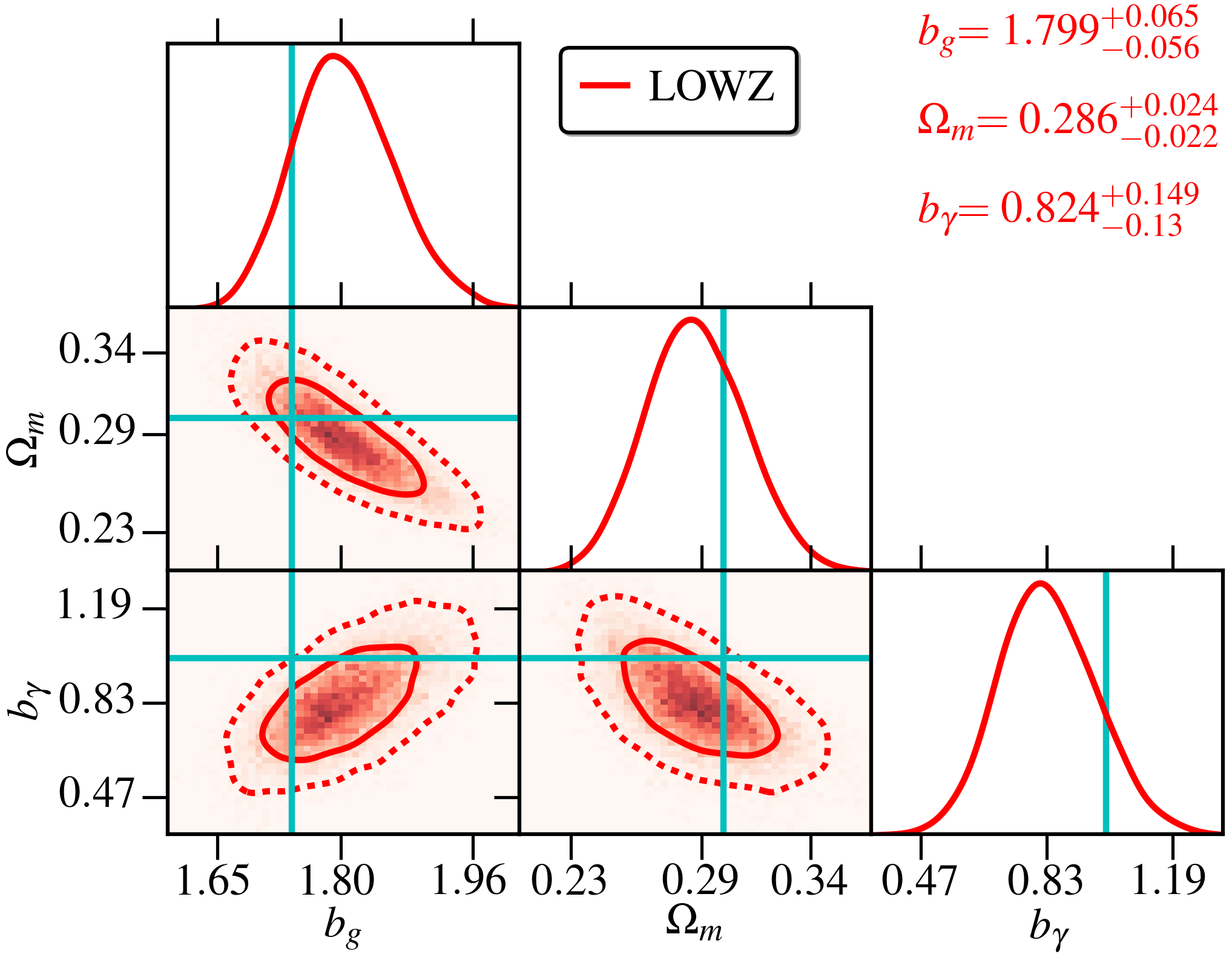
In Fig. 12, we show the results from jointly fitting the galaxy clustering, CMB lensing and galaxy lensing signals for the LOWZ sample using the MCMC fitting method. We fit for linear galaxy bias , and , where is the relative calibration bias between CMB lensing and galaxy lensing (CMB lensing amplitude , and galaxy lensing amplitude ). Our result of is consistent with , which would imply no difference in calibration between the two lensing methods, at level. Note that the value from MCMC fits, differs from the jackknife fits, , shown earlier for two main reasons: the lower value of (fixed to ) in jackknife fits; and we do not use the RSD corrections in the MCMC fits to speed up computation time, moving higher by ( for jackknife fitting without RSD correction). The RSD correction is at the scales we use (Baldauf et al., 2010), which is much less than the statistical uncertainties in both and . A more detailed cosmological analysis using these measurements with improved modeling on small scales will be presented in a forthcoming paper (Singh et al. in prep).
4.4 Cosmography
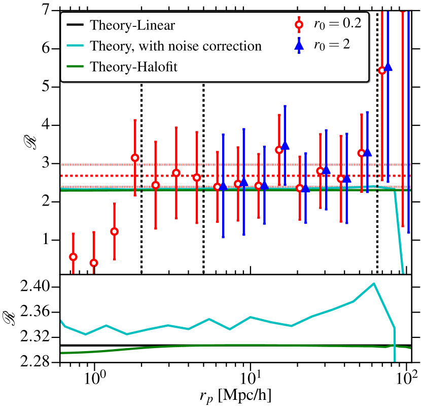
In Fig. 13, we present the measurement of the distance ratio as defined in Eq. (42). We present the measurement using two different values of : and . As was discussed in Sec. 2.7, it is desirable to use in estimating , to avoid the information from scales where the smoothing of the CMB lensing map is important. Using accomplishes this goal, while the case is equivalent to taking ratios using when using scales . The sudden drop in measured below when using is consistent with expectations from the effects of smoothing. As discussed in Sec. 2.7, the effects of non-linear growth also lead to lower on small scale by giving higher weights to lower redshifts (where is lower), though this is effect is estimated to be much smaller than the statistical uncertainties in our measurements ( at ). Using the “aggressive” range, with , the mean value of is , consistent with the predicted value of from the Planck 2015 cosmology. Including the effects of noise in our theory prediction as described in Sec. 2.7, the prediction becomes using realizations with noise and scales from and . Using a more conservative range of scales, with , we get , with the prediction . However, given the strong agreement between our results with conservative and aggressive choices of and scales for the measurement, we quote as our primary result. We do not use as these scales are larger than the size of jackknife regions and hence the covariance matrix is not very reliable at these scales.
We do not derive any cosmological constraints using since it is not very sensitive to cosmological parameters given the redshift distribution of our lens and source redshifts (Hu et al., 2007b).
4.5 Lensing-lensing correlations
In this section we present the results of cross-correlating the Planck lensing map with the galaxy shear from the SDSS shape sample (Reyes et al., 2012; Nakajima et al., 2012), using the estimator presented in Sec. 2.2.
In Fig. 14, we present the lensing-lensing cross-correlations with two different choices of pixel sizes. We fit the signal to a constant times the predictions for the Planck 2015 cosmology, for (to avoid scales where noise starts dominating). The best-fitting amplitudes, (n=512) and (n=1024), which are consistent with the Planck 2015 cosmological parameters () at level, for both pixel sizes. If we relax the fit limits to , the amplitude decreases to , which is in tension but still consistent with the Planck 2015 cosmological parameters at level. The shift between the fits using the more conservative and aggressive ranges of is less than after accounting for the correlations between the values for these two cases, and may be an effect of large-scale systematics at large scales. In the lensing-lensing cross-correlations, is (in principle) also a quantity with zero mean and hence the estimator is less prone to the effects of correlated noise. However, also has some residual additive systematics at large scales (Mandelbaum et al., 2013), making it a quantity with non-zero mean on large scales; it can therefore combine with the correlated noise (or systematics) in the CMB convergence maps to give some residual systematics in the cross-correlations. 333It is known that shear has systematics, so that measured shear, . The measured cross-correlation with galaxies is then , where is the systematics term in galaxy-galaxy lensing and is removed by subtracting measurement around randoms. Now, lets consider simple case in which CMB convergence also has some additive systematic, so that , where we assume is constant and same in all pixels. In galaxy-CMB lensing, this systematic also gets removed when measurement around randoms is subtracted. The correlation with shear is then, . The can bias the shear-convergence cross correlation measurements. As discussed later in this section, we do not find any evidence of systematics in our null tests, though the uncertainties in our measurements are large. In this work we do not attempt to construct a better estimator given the noise in our measurements. In future works, with better signal-to-noise, it will be worth exploring a better estimator that removes the effects of residual additive systematics.
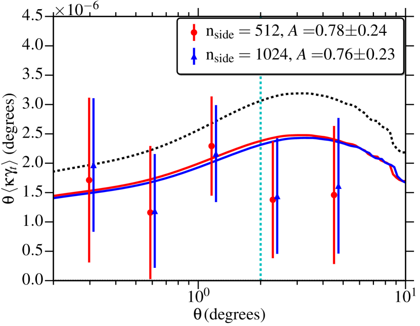
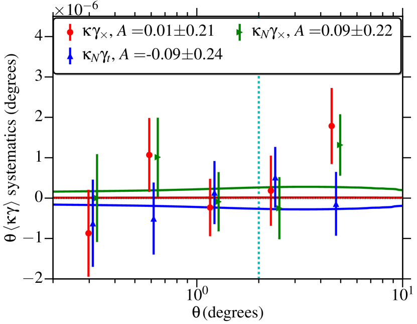
Fig. 15 shows several null tests used to uncover the effects of systematic errors. The first is the ‘B-mode’ signal , which is expected to be zero from parity conservation. As a test, we fit to a model consisting of a constant times the prediction for from the Planck 2015 cosmology; this gives , consistent with as expected. Similarly, we repeat the measurement by replacing the Planck convergence with the noise map to compute and , and using the shuffled convergence map (not shown, ). All of these measurements give consistent with zero.
While the deviations from the predictions using the Planck 2015 cosmology are not statistically significant, it is worth noting that there are several possible systematics that could bias the amplitude of this cross-correlation, for example, intrinsic alignments (IA) and biases in the redshift distributions. Chisari et al. (2015) estimated the contribution from IA contamination in the CMB vs. galaxy lensing cross-correlations to be around for the CFHT stripe 82 survey. Since the SDSS source sample is shallower than the stripe 82 sample and hence at lower effective redshift, the fractional IA contamination can be higher. This statement assumes the validity of the linear alignment model (Hirata & Seljak, 2003), which has been shown to describe the IA of red galaxies, and which predicts that the IA signal is approximately constant with redshift while the lensing cross-correlation signal with the CMB decreases at lower redshift. The IA contamination also depends on the galaxy luminosity (fainter galaxies have lower IA) and on the fraction of red galaxies in the sample (here we ignore alignments for spiral galaxies since all current measurements of IA for spirals are consistent with zero). Assuming a sample with galaxies to be LOWZ-like LRGs (effective IA amplitude ), we predict a contamination of . This is a conservative upper limit considering that our source sample is much fainter than the LOWZ sample and is dominated by blue galaxies. See also Blazek et al. (2012) who constrained IA contamination in galaxy-galaxy lensing measurements to be less than 5% using the same source sample as this work.
Regarding photo- systematics and redshift uncertainties, their impact on galaxy-galaxy lensing for this shear catalogue was quantified using a complete and representative spectroscopic sample in Nakajima et al. (2012), who found per cent uncertainties in the mean and therefore lensing amplitude. To check whether the difference may be more significant here, we considered the difference in the best-fitting amplitude when we make the theoretical predictions using the redshifts from the calibration sample from Nakajima et al. (2012), vs. when we make them from a smooth parametric fit to the histogram, and find per cent uncertainties. We therefore conclude that redshift uncertainty is a subdominant contributor to the error budget for the lensing-lensing correlations. The same may not be true in future datasets for which a representative spectroscopic sample is not available.
5 Conclusions
In this paper we have presented results from cross-correlating Planck CMB lensing maps with shear from SDSS galaxy lensing and galaxy positions from the SDSS-III BOSS survey using both the LOWZ and higher redshift CMASS sample.
Cross-correlating galaxy positions with the convergence maps, we detect the CMB lensing signal around galaxies out to . The measured signals are consistent with predictions using the Planck 2015 cosmology with bias measurements from clustering. Our null tests do not reveal any significant evidence for systematics in our measurements. The mild tensions between data and theory, e.g., for CMASS sample, are likely due to noise fluctuations, particularly given that there is no tension observed for the LOWZ sample.
We also detected the CMB lensing signal around galaxies at very small separations, well below the effective smoothing scale of 6′ in the convergence maps. Combining the clustering measurements with NFW profiles and then applying the smoothing kernel, we are able to constrain halo mass at the 3–4 level for different samples, though the halo masses could be biased given the simple adopted model.
We directly compared the lensing signal around LOWZ galaxies obtained from galaxy-lensing and CMB-lensing. We find that the galaxy lensing has a better signal-to-noise ratio by a factor of 2–5, depending on the scale. Combining these measurements with the galaxy clustering signal, we also performed a basic cosmological analysis jointly fitting for , galaxy bias, and the relative calibration bias between galaxy and CMB lensing. We find , consistent with the Planck 2015 cosmology at the level. We find the relative calibration bias between galaxy lensing and CMB lensing to be , consistent with 1 at just over . In addition, we also measured the distance ratio between the lens and source galaxies and the CMB last scattering surface to within %. The ratio is consistent with the prediction using Planck 2015 cosmology; unfortunately, this ratio is not strongly sensitive to cosmology given the low lens redshift, and hence does not provide competitive cosmological constraints.
For lensing-lensing cross-correlations, we detected the signal at significance at an effective redshift of 0.35. The amplitude of the signal is consistent with model predictions using Planck 2015 cosmology. Given the noise in this measurement, we expect systematic errors such as intrinsic alignments and uncertainties in the source galaxy redshift distribution to be subdominant components of the error budget. We also performed null tests, which did not show any evidence for systematics within the errorbars.
To conclude, our results demonstrate how CMB lensing data can be incorporated into and combined with the galaxy lensing analysis using existing lensing surveys. Even though the CMB lensing measurements are noisier than galaxy lensing and will perhaps remain so for the near future, existing CMB lensing measurements are already good enough to provide strong consistency checks on galaxy lensing measurements. This analysis is an important proof of concept for future surveys that plan to use CMB lensing in conjunction with galaxy lensing, as an additional high-redshift lens plane with completely independent systematics. With better resolution in the upcoming lensing results from current generation and Stage IV CMB surveys, CMB lensing can also develop into a unique tool to study dark matter at higher redshifts, to which it is most sensitive, and which will remain beyond the reach of currently planned galaxy lensing surveys.
Acknowledgments
We thank François Lanusse, Anthony Pullen, Alex Geringer-Sameth, Sébastien Fromenteau and Shirley Ho for useful discussions related to this work. We also thank Uroš Seljak, Emmanuel Schaan, David Spergel and the anonymous referee for helpful feedback on this work. We thank Martin White and Beth Reid for providing us halo catalog from simulations. We also thank the SDSS-I/II/III and Planck collaboration for their efforts in providing the datasets used in this work.
RM acknowledges the support of the Department of Energy Early Career Award program. SS acknowledges support from John Peoples Jr. Presidential Fellowship from Carnegie Mellon University.
Some of the results in this paper have been derived using the HEALPix package (Górski et al., 2005).
Funding for SDSS-III has been provided by the Alfred P. Sloan Foundation, the Participating Institutions, the National Science Foundation, and the U.S. Department of Energy Office of Science. The SDSS-III web site is http://www.SDSS3.org/.
SDSS-III is managed by the Astrophysical Research Consortium for the Participating Institutions of the SDSS-III Collaboration including the University of Arizona, the Brazilian Participation Group, Brookhaven National Laboratory, Carnegie Mellon University, University of Florida, the French Participation Group, the German Participation Group, Harvard University, the Instituto de Astrofisica de Canarias, the Michigan State/Notre Dame/JINA Participation Group, Johns Hopkins University, Lawrence Berkeley National Laboratory, Max Planck Institute for Astrophysics, Max Planck Institute for Extraterrestrial Physics, New Mexico State University, New York University, Ohio State University, Pennsylvania State University, University of Portsmouth, Princeton University, the Spanish Participation Group, University of Tokyo, University of Utah, Vanderbilt University, University of Virginia, University of Washington, and Yale University.
Author Contributions: SS and RM contributed to the analysis and writing the paper. JB is an SDSS-III BOSS architect who contributed to the development of the BOSS survey.
References
- Abazajian et al. (2009) Abazajian K. N., et al., 2009, ApJS, 182, 543
- Ade et al. (2014) Ade P. A. R., et al., 2014, Physical Review Letters, 113, 021301
- Ahn et al. (2012) Ahn C. P., et al., 2012, ApJS, 203, 21
- Aihara et al. (2011) Aihara H., et al., 2011, ApJS, 193, 29
- Alam et al. (2015) Alam S., et al., 2015, ApJS, 219, 12
- Baldauf et al. (2010) Baldauf T., Smith R. E., Seljak U., Mandelbaum R., 2010, Phys.Rev.D, 81, 063531
- Bartelmann & Schneider (2001) Bartelmann M., Schneider P., 2001, Phys.Rep., 340, 291
- Baxter et al. (2015) Baxter E. J., et al., 2015, ApJ, 806, 247
- Bernstein & Jain (2004) Bernstein G., Jain B., 2004, ApJ, 600, 17
- Bernstein & Jarvis (2002) Bernstein G. M., Jarvis M., 2002, AJ, 123, 583
- Bhattacharya et al. (2013) Bhattacharya S., Habib S., Heitmann K., Vikhlinin A., 2013, ApJ, 766, 32
- Bianchini et al. (2015) Bianchini F., et al., 2015, preprint, (arXiv:1511.05116)
- Blanton et al. (2003) Blanton M. R., Lin H., Lupton R. H., Maley F. M., Young N., Zehavi I., Loveday J., 2003, AJ, 125, 2276
- Blazek et al. (2012) Blazek J., Mandelbaum R., Seljak U., Nakajima R., 2012, J. Cosmology Astropart. Phys., 5, 41
- Bleem et al. (2012) Bleem L. E., et al., 2012, ApJ, 753, L9
- Bolton et al. (2012) Bolton A. S., et al., 2012, AJ, 144, 144
- Caminha et al. (2016) Caminha G. B., et al., 2016, A&A, 587, A80
- Chisari et al. (2015) Chisari N. E., Dunkley J., Miller L., Allison R., 2015, MNRAS, 453, 682
- Das et al. (2011) Das S., et al., 2011, Physical Review Letters, 107, 021301
- Das et al. (2013) Das S., Errard J., Spergel D., 2013, preprint, (arXiv:1311.2338)
- Das et al. (2014) Das S., et al., 2014, J. Cosmology Astropart. Phys., 4, 014
- Dawson et al. (2013) Dawson K. S., et al., 2013, AJ, 145, 10
- Diego et al. (2015) Diego J. M., et al., 2015, MNRAS, 446, 683
- Diemer & Kravtsov (2015) Diemer B., Kravtsov A. V., 2015, ApJ, 799, 108
- Eisenstein et al. (2001) Eisenstein D. J., et al., 2001, AJ, 122, 2267
- Erben et al. (2013) Erben T., et al., 2013, MNRAS, 433, 2545
- Feldmann et al. (2006) Feldmann R., et al., 2006, MNRAS, 372, 565
- Fukugita et al. (1996) Fukugita M., Ichikawa T., Gunn J. E., Doi M., Shimasaku K., Schneider D. P., 1996, AJ, 111, 1748
- Giannantonio & Percival (2014) Giannantonio T., Percival W. J., 2014, MNRAS, 441, L16
- Giannantonio et al. (2016) Giannantonio T., et al., 2016, MNRAS, 456, 3213
- Golse et al. (2002) Golse G., Kneib J.-P., Soucail G., 2002, A&A, 387, 788
- Górski et al. (2005) Górski K. M., Hivon E., Banday A. J., Wandelt B. D., Hansen F. K., Reinecke M., Bartelmann M., 2005, ApJ, 622, 759
- Gunn et al. (1998) Gunn J. E., et al., 1998, AJ, 116, 3040
- Gunn et al. (2006) Gunn J. E., et al., 2006, AJ, 131, 2332
- Hand et al. (2015) Hand N., et al., 2015, Phys.Rev.D, 91, 062001
- Harnois-Déraps et al. (2016) Harnois-Déraps J., et al., 2016, MNRAS,
- Hirata & Seljak (2003) Hirata C., Seljak U., 2003, MNRAS, 343, 459
- Hirata et al. (2008) Hirata C. M., Ho S., Padmanabhan N., Seljak U., Bahcall N. A., 2008, Phys.Rev.D, 78, 043520
- Hogg et al. (2001) Hogg D. W., Finkbeiner D. P., Schlegel D. J., Gunn J. E., 2001, AJ, 122, 2129
- Hu & Okamoto (2002) Hu W., Okamoto T., 2002, ApJ, 574, 566
- Hu et al. (2007a) Hu W., DeDeo S., Vale C., 2007a, New Journal of Physics, 9, 441
- Hu et al. (2007b) Hu W., Holz D. E., Vale C., 2007b, Phys.Rev.D, 76, 127301
- Ivezić et al. (2004) Ivezić Ž., et al., 2004, Astronomische Nachrichten, 325, 583
- Jain & Taylor (2003) Jain B., Taylor A., 2003, Physical Review Letters, 91, 141302
- Kaiser (1987) Kaiser N., 1987, MNRAS, 227, 1
- Keck Array et al. (2016) Keck Array T., et al., 2016, preprint, (arXiv:1606.01968)
- Kirk et al. (2016) Kirk D., et al., 2016, MNRAS, 459, 21
- Kitching et al. (2015) Kitching T. D., et al., 2015, preprint, (arXiv:1512.03627)
- Landy & Szalay (1993) Landy S. D., Szalay A. S., 1993, ApJ, 412, 64
- Lewis & Bridle (2002) Lewis A., Bridle S., 2002, Phys. Rev., D66, 103511
- Lewis & Challinor (2006) Lewis A., Challinor A., 2006, Phys.Rep., 429, 1
- Link & Pierce (1998) Link R., Pierce M. J., 1998, ApJ, 502, 63
- Liu & Hill (2015) Liu J., Hill J. C., 2015, Phys.Rev.D, 92, 063517
- Liu et al. (2016) Liu J., Ortiz-Vazquez A., Hill J. C., 2016, preprint, (arXiv:1601.05720)
- Lupton et al. (2001) Lupton R., Gunn J. E., Ivezić Z., Knapp G. R., Kent S., 2001, in Harnden Jr. F. R., Primini F. A., Payne H. E., eds, Astronomical Society of the Pacific Conference Series Vol. 238, Astronomical Data Analysis Software and Systems X. p. 269 (arXiv:astro-ph/0101420)
- Madhavacheril et al. (2015) Madhavacheril M., et al., 2015, Physical Review Letters, 114, 151302
- Mandelbaum et al. (2005) Mandelbaum R., et al., 2005, MNRAS, 361, 1287
- Mandelbaum et al. (2006) Mandelbaum R., Hirata C. M., Ishak M., Seljak U., Brinkmann J., 2006, MNRAS, 367, 611
- Mandelbaum et al. (2011) Mandelbaum R., et al., 2011, MNRAS, 410, 844
- Mandelbaum et al. (2013) Mandelbaum R., Slosar A., Baldauf T., Seljak U., Hirata C. M., Nakajima R., Reyes R., Smith R. E., 2013, MNRAS, 432, 1544
- Manera et al. (2015) Manera M., et al., 2015, MNRAS, 447, 437
- Miyatake et al. (2015) Miyatake H., et al., 2015, ApJ, 806, 1
- Miyatake et al. (2016) Miyatake H., Madhavacheril M. S., Sehgal N., Slosar A., Spergel D. N., Sherwin B., van Engelen A., 2016, preprint, (arXiv:1605.05337)
- More et al. (2015) More S., Miyatake H., Mandelbaum R., Takada M., Spergel D. N., Brownstein J. R., Schneider D. P., 2015, ApJ, 806, 2
- Nakajima et al. (2012) Nakajima R., Mandelbaum R., Seljak U., Cohn J. D., Reyes R., Cool R., 2012, MNRAS, 420, 3240
- Navarro et al. (1996) Navarro J. F., Frenk C. S., White S. D. M., 1996, ApJ, 462, 563
- Padmanabhan et al. (2008) Padmanabhan N., et al., 2008, ApJ, 674, 1217
- Pier et al. (2003) Pier J. R., Munn J. A., Hindsley R. B., Hennessy G. S., Kent S. M., Lupton R. H., Ivezić Ž., 2003, AJ, 125, 1559
- Planck Collaboration et al. (2014) Planck Collaboration et al., 2014, A&A, 571, A17
- Planck Collaboration et al. (2015c) Planck Collaboration et al., 2015c, preprint, (arXiv:1502.01589)
- Planck Collaboration et al. (2015a) Planck Collaboration et al., 2015a, preprint, (arXiv:1502.01591)
- Planck Collaboration et al. (2015b) Planck Collaboration et al., 2015b, preprint, (arXiv:1502.01597)
- Pullen et al. (2015) Pullen A. R., Alam S., He S., Ho S., 2015, preprint, (arXiv:1511.04457)
- Reid & Spergel (2009) Reid B. A., Spergel D. N., 2009, ApJ, 698, 143
- Reid et al. (2014) Reid B. A., Seo H.-J., Leauthaud A., Tinker J. L., White M., 2014, MNRAS, 444, 476
- Reid et al. (2016) Reid B., et al., 2016, MNRAS, 455, 1553
- Reyes et al. (2012) Reyes R., Mandelbaum R., Gunn J. E., Nakajima R., Seljak U., Hirata C. M., 2012, MNRAS, 425, 2610
- Richards et al. (2002) Richards G. T., et al., 2002, AJ, 123, 2945
- Rodríguez-Torres et al. (2016) Rodríguez-Torres S. A., et al., 2016, MNRAS,
- Ross et al. (2012) Ross A. J., et al., 2012, MNRAS, 424, 564
- Sheldon et al. (2004) Sheldon E. S., et al., 2004, AJ, 127, 2544
- Sherwin et al. (2012) Sherwin B. D., et al., 2012, Phys.Rev.D, 86, 083006
- Singh et al. (2015) Singh S., Mandelbaum R., More S., 2015, MNRAS, 450, 2195
- Smee et al. (2013) Smee S. A., et al., 2013, AJ, 146, 32
- Smith et al. (2002) Smith J. A., et al., 2002, AJ, 123, 2121
- Smith et al. (2003) Smith R. E., et al., 2003, MNRAS, 341, 1311
- Smith et al. (2007) Smith K. M., Zahn O., Doré O., 2007, Phys.Rev.D, 76, 043510
- Strauss et al. (2002) Strauss M. A., et al., 2002, AJ, 124, 1810
- Takahashi et al. (2012) Takahashi R., Sato M., Nishimichi T., Taruya A., Oguri M., 2012, ApJ, 761, 152
- Taylor et al. (2012) Taylor J. E., et al., 2012, ApJ, 749, 127
- Taylor et al. (2013) Taylor A., Joachimi B., Kitching T., 2013, MNRAS, 432, 1928
- Tucker et al. (2006) Tucker D. L., et al., 2006, Astronomische Nachrichten, 327, 821
- Vallinotto (2012) Vallinotto A., 2012, ApJ, 759, 32
- Wake et al. (2006) Wake D. A., et al., 2006, MNRAS, 372, 537
- Weinberg et al. (2013) Weinberg D. H., Mortonson M. J., Eisenstein D. J., Hirata C., Riess A. G., Rozo E., 2013, Phys.Rep., 530, 87
- York et al. (2000) York D. G., et al., 2000, AJ, 120, 1579
- Zaldarriaga & Seljak (1999) Zaldarriaga M., Seljak U., 1999, Phys.Rev.D, 59, 123507
- Zheng et al. (2005) Zheng Z., et al., 2005, ApJ, 633, 791
- de Putter et al. (2014) de Putter R., Doré O., Das S., 2014, ApJ, 780, 185
- van Engelen et al. (2012) van Engelen A., et al., 2012, ApJ, 756, 142
- van Engelen et al. (2014) van Engelen A., Bhattacharya S., Sehgal N., Holder G. P., Zahn O., Nagai D., 2014, ApJ, 786, 13
- van den Bosch et al. (2013) van den Bosch F. C., More S., Cacciato M., Mo H., Yang X., 2013, MNRAS, 430, 725
Appendix A Effect of weights in the CMASS sample
In this section we briefly discuss the effect of using weights in measurements involving the CMASS sample.
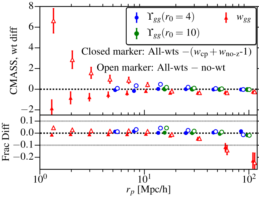
Fig. 16 shows the difference in clustering measurements done with and without using weights. The effect of the systematics weights is to shift lower by an additive factor that has only a weak scale dependence; this effect is the dominant impact of the weights on large scales. Since clustering varies very strongly with scale, the fractional change in clustering increases very strongly with scale. The weights for redshift failure up-weight the higher density regions and hence change the clustering strongly at small scales, while the change in the large-scale bias is small ().
by definition will not be very strongly affected by additive changes in . Fig. 16 demonstrates the fact that the fractional change in from systematics weights is , even on scales where the fractional change in is . At the scales that dominate our constraints in (), the fractional change in without vs. with systematics weights is , below the statistical errors. As a result, our constraints from do not depend on the choice of whether or not to use systematics weights. The redshift failure weights change the clustering by a strongly scale-dependent factor, so is affected in nearly the same way as . However, the effect on scales we use for the fits for large-scale bias is small, so the change in linear galaxy bias is again .
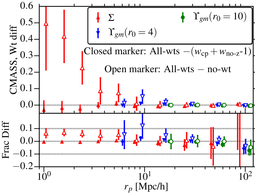
In Fig. 17 we show the effect of using weights on the lensing measurements with Planck convergence maps. Given the noise in the lensing measurements, the systematics weights do not affect the measurements very significantly and the fractional change in lensing is at all scales, less than the statistical errors in the measurements. The redshift incompleteness weights change the small scale signal in a similar way as in the clustering measurement, by up-weighting the higher density regions, though the shift at large scales is small and negligible given the larger noise in the lensing measurements.
Appendix B Comparison of different error estimates
Here we present a brief comparison of errors in the CMB lensing measurements obtained using the jackknife method with the errors obtained using the scatter between 100 random realizations of the noise map .
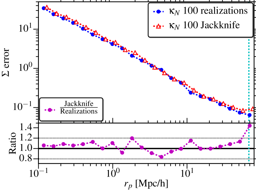
In Fig. 18, we show the comparison of the error bars (square root of diagonal elements of covariance matrix, ) in from these two methods. The errors obtained using the two methods are consistent to within 20% (% on most scales), with the jackknife errors being larger on most scales. The relative uncertainty in the errors, (Taylor et al., 2013), which predicts scatter (assuming two estimates are independent) when taking the ratio of errors obtained using the two methods. Thus we can conclude that the errors obtained using the two methods are consistent. In Fig. 19, we show the correlation matrix obtained from the two estimation methods; they are consistent within the noise.
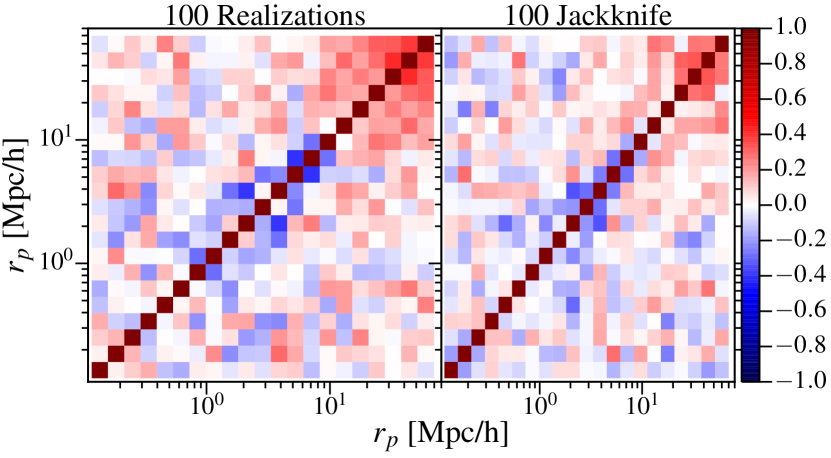
We also tested the covariance matrices by varying the number of random points. We find correlation matrices that are consistent when using a number of random points , with ; the variation in the error on (square root of diagonal of covariance) is between these cases. We use for our main results.