Effect of compactification of twisted toroidal extra-dimension on sterile neutrino

Abstract

We consider a toroidal extra-dimensional space with shape moduli $\theta$ which is the angle between the two large extra dimensions $R_{1}$ and $R_{2}$ (twisted LED with $\delta=2$). The Kaluza-Klein (KK) compactification results in a tower of KK bulk neutrinos which are sterile in nature and couple to the active neutrinos in the brane. The active-sterile mixing probability strongly depends on the angle $\theta$ due to changing pattern of KK mass gaps which leads to level crossing. Considering only the first two lowest KK states in analogy with $(3+2)$ model, it is shown that $|U_{\alpha 4}|>|U_{\alpha 5}|$ when $\theta=\pi/2$ corresponding to the case of a normal torus. Since $\Delta_{14}^{2}<\Delta_{15}^{2}$, this is expected in normal LED model as higher the sterile mass lower is the mixing probability. Contrary to this expectation, it is found that there exists a range in $\theta$ where $|U_{\alpha 5}|\geq|U_{\alpha 4}|$ even though $\Delta m_{14}^{2}<\Delta m_{15}^{2}$ which has been demonstrated qantitatively using fourier transformation of reactor anti-neutrino spectrum. This is an important observation which can be linked to the oscillation parameters extracted by several $(3+2)$ global analyses of the neutrino and anti-neutrino data obtained from the short base line measurements.

I Introduction

We consider the compactification of toroidal two extra dimensions characterised by a shape moduli $\theta$ which is the angle bewteen the two large extra dimensions $R_{1}$ and $R_{2}$. The non trivial effect of shape moduli on compactification was first studied by Dienes and Mafi who brought out a number of profound phenomena relevant for the interpretation of experimental data if such extra dimensions exist Dienes_prl1 ; Dienes_prl2 . Notably among them is the changing pattern of Kaluza-Klein (KK) mass gaps which strongly depend on $\theta$ and exhibit level crossing making some of the higher KK modes lighter as compared to the lower ones when $\theta$ is varied. This is an important aspect which we incorporate in the ADD (Arkani-Hamed, Dimopoulos and Dvali) model with two large extra dimensions (LED) to study the active-sterile neutrino mixing in $4+\delta$ dimensions with $\delta=2$ ADD1 ; ADD2 . Another impetus to this work stems from the recent observation that the fit to the short base line (SBL) reactor anti-neutrino measurements with new anti-neutrino flux muller ; huber improves considerably if two sterile neutrions $(3+2)$ are assumed instead of one $(3+1)$ Kopp_prl . Naively, it is observed that $\Delta m_{51}$ is about $\sqrt{2}$ times larger than $\Delta m_{41}$ and $|U_{15}|\geq|U_{14}|$ Kopp_prl ; Kopp1 . The LED model with $\delta=1$ (one extra dimension larger than others) results in a tower of KK sterile neutrions with KK mass increasing as $n$ and mixing probability decreasing as $1/n^{2}$ where $n=1,2,3$ etc Anton ; ADD3 ; Dienes ; Dvali ; Bar ; Davo ; Gin ; Cao ; Gonzalez ; Rode . Obviously, the case with $\delta=1$ is not consistent with the above observations if we consider first two lowest sterile states. In case of $\delta=2$, the KK mass increases as $\sqrt{m^{2}+n^{2}}$ where $m$ and $n$ are two different KK modes associated with $R_{1}$ and $R_{2}$ respectively. Although the mass of first two KK modes $(1,0)$ or $(0,1)$ and $(1,1)$ differ by a factor of $\sqrt{2}$, as expected, still it does not predict the observed active-sterile mixing probability when $\theta=\pi/2$. On the other hand, when $\theta$ is close to $\pi/4$, the predicted masses and mixing probabilities are found to be consistent with the above experimental obsevations. In this letter, we consider compactification on a general two-torus corresponding to $\delta=2$ instead of $\delta=1$ as one dimensional compactification lacks shape moduli. It is shown here that there exists a range in $\theta$ where $|U_{\alpha 5}|\geq|U_{\alpha 4}|$ even though $\Delta m_{14}^{2}<\Delta m_{15}^{2}$. This is an important observation which is demonstrated more quantitatively using cosine Fourier transformation of the reactor anti-neutrino spectra.

II Formalism

We consider a brane world theory with $6$ dimensional bulk, where the active neutrinos are confined to the brane and the singlet sterile neutrino $\Phi^{\alpha}(x^{\mu},y_{1},y_{2})$ propagates in the bulk with extra dimensions $y_{1}$ and $y_{2}$. Using the Kaluza-Klein (KK) expansion, the singlet fermionic field can be expanded as,

$$\Phi_{R/L}(x^{\mu},y)\sum_{m}\sum_{n}\Phi_{R/L}^{(m,n)}(x^{\mu})~{}f^{mn}(y_{1},y_{2}),$$ (1)

where $\mu=0,1,2,3$ are co-ordinates belonging to the brane and $y_{1},~{}y_{2}$ are the co-ordinates of two extra dimensions. The subscripts $R$ and $L$ refer explicitly to four dimensional Lorentz property. The periodic function $f^{mn}(y_{1},y_{2})$ is given by,

$$f^{mn}(y_{1},y_{2})=\frac{1}{\sqrt{V}}exp\left[i\frac{m}{R_{1}}\left(y_{1}-\frac{y_{2}}{tan\theta}\right)+i\frac{n}{R_{2}}\frac{y_{2}}{sin\theta}\right],$$ (2)

with periodicity $y_{1}\sim y_{1}+2\pi(R_{1}+R_{2}cos\theta)$ and $y_{2}\sim y_{2}+2\pi R_{2}sin\theta$ Dienes_prl1 . The normalization factor $V=4\pi^{2}R_{2}sin\theta(R_{1}+R_{2}cos\theta)$ plays the role of volume of the extra-dimensions. Note that for $\theta=\pi/2$, $V=4\pi^{2}R_{1}R_{2}$ which is the volume of a normal torus. Eq. 2 satisfies the condition,

$$\frac{1}{V}\int_{0}^{\infty}\left(f^{pq}\right)^{*}f^{mn}dy_{1}dy_{2}=\delta_{pm}\delta_{qn}.$$ (3)

The bulk action responsible for the neutrino mass is given by (kinetic term is not included) Dudas ,

$$A_{bulk}=\int d^{4}x~{}dy_{1}~{}dy_{2}~{}\big{[}\Phi_{L}^{\dagger}(\partial_{5}+i\partial_{6})\Phi_{R}-\Phi_{R}^{\dagger}(\partial_{5}-i\partial_{6})\Phi_{L}\big{]}.$$ (4)

Using Eq. 1, Eq. 2, Eq. 3 and the substitution,

$$\Psi_{R}^{0,0}=\Phi_{R}^{0,0}~{}~{};~{}~{}\Psi_{R}^{m,n}=\frac{1}{\sqrt{2}}\left(\Phi_{R}^{m,n}+\Phi_{R}^{-m,-n}\right)~{}~{};~{}~{}\Psi_{L}^{m,n}=\frac{1}{\sqrt{2}}\left(\Phi_{L}^{m,n}+\Phi_{L}^{-m,-n}\right),$$ (5)

the $y_{1}$ and $y_{2}$ variable in Eq. 4 can be integrated out to get,

$$A_{bulk}=-\int d^{4}x\sum_{m,n}^{N}\frac{k_{m,n}}{R}\big{(}\Psi_{R}^{(m,n)\dagger}\Psi_{L}^{(m,n)}+\Psi_{L}^{(m,n)\dagger}\Psi_{R}^{(m,n)}\big{)},$$ (6)

where the absolute value of the mass term for $(m,n)$ mode is given by,

$$k_{m,n}=\sqrt{\frac{1}{sin\theta}\left(m^{2}+n^{2}-2m~{}n~{}cos\theta\right)}.$$ (7)

We have relaxed the condition further by assuming that $R_{1}=R_{2}=R$. Note that the summation $\sum_{mn}$ above is over all modes of $m$ and $n$ upto a maximum value of $N$, but excluding $m=n=0$ mode. We can now add the relevant portion of interaction term between brane and the bulk field containg mass,

$$A_{int}=-m_{D}\int d^{4}x\bigg{[}\nu_{L}^{\dagger}\bigg{(}\nu_{R}+\sqrt{2}\sum_{m,n}^{N}\Psi_{R}^{(m,n)}\bigg{)}+hc\bigg{]}$$ (8)

where $\nu_{R}=\Psi_{R}^{(0,0)}$ and $m_{D}$ is the Dirac neutrino mass generated due to coupling of bulk neutrinos with the brane localized SM Higgs boson at $y_{1}=y_{2}=0$. Finally, by collecting the neutrino mass terms in the Lagrangian and explicitly including the neutrino flavor indices $\alpha$ and $\beta$, we obtain,

$$\mathcal{L}_{mass}=-\sum_{\alpha=1}^{3}\sum_{m,n}^{N}\frac{k_{m,n}}{R}\Psi_{R}^{\alpha(m,n)\dagger}\Psi_{L}^{\alpha(m,n)}-\sum_{\alpha,\beta=1}^{3}m_{D}^{\alpha\beta}\bigg{(}\nu_{R}^{\alpha\dagger}+\sqrt{2}\sum_{m,n}^{N}\Psi_{R}^{\alpha(m,n)\dagger}\bigg{)}\nu_{L}^{\beta}+hc$$ (9)

Note that while the right handed sterile neutrino $\Psi_{R}^{0,0}$ participates in the process of mass generation at the brane, the left handed sterile neutrino $\Psi_{L}^{0,0}$ decouples from the mass part of the Lagrangian as $k_{mn}$ vanishes for $(0,0)$ mode. We also neglect the Majrona mass and associate suitable lepton number to $\Psi_{R}$ so that lepton number is conserved. The formalism is now similar to the case of $\delta=1$ and can be found in several works Anton ; ADD3 ; Dienes ; Dvali ; Bar ; Davo ; Gin ; Cao ; Gonzalez ; Rode . Therefore, following the standard procedure of diagonalizing the Dirac mass term $m^{\alpha\beta}$ with PMNS matrx $U$ and making a symmetric transformation to a set of new basis, the mass Lagrangian can be written in a compact form given by Dienes ; Cao ,

$$\mathcal{L}_{mass}=\frac{1}{2}\bigg{(}\nu^{\dagger}\it{M}\nu+hc\bigg{)},$$ (10)

where the neutrino mass matrix $M$ is given by,

$$M=\left(\begin{array}[]{ccccccc}0&m_{\nu}&m_{\nu}&m_{\nu}&m_{\nu}&\cdots&m_{\nu}\\ m_{\nu}&0&0&0&0&\cdots&0\\ \vdots&\vdots&\vdots&\vdots&\vdots&\vdots&\vdots\\ m_{\nu}&0&\frac{k_{mn}}{R}&0&0&\cdots&0\\ m_{\nu}&0&0&-\frac{k_{mn}}{R}&0&\cdots&0\\ \vdots&\vdots&\vdots&\vdots&\vdots&\vdots&\vdots\\ m_{\nu}&0&0&0&\cdots&\frac{k_{NN}}{R}&0\\ m_{\nu}&0&0&0&0&\cdots&-\frac{k_{NN}}{R}\\ \end{array}\right),$$ (19)

with $\nu=(\nu_{L},\nu_{R},\nu_{s}^{-1},\nu_{s}^{1}\cdots)^{T}$. In the above, the Dirac mass $m_{\nu}$ could be either $m_{1}$, $m_{2}$ or $m_{3}$ depending on whether it is $e$, $\mu$ or $\tau$ neutrino. The mass term $k_{mn}/R$ appearing in Eq. 19 represents ($d_{k}\times d_{k}$) block diagonal matrix, $d_{k}$ being the degeneracy of the $(m,n)$ mass state, $N$ is the upper limit of $m$ or $n$. For $N=1$, the independent modes are $(1,0)$ and $(1,1)$ since $(0,1)$ and $(1,0)$ mode degenerates. Similarly for $N=2$, the independent modes are $(0,1)_{d=2}$, $(1,1)$, $(2,0)_{d=2}$, $(1,2)_{d=2}$ and $(2,2)$. Therefore, for the case of $\delta=2$, $d$ is either $2$ or $1$. Finally, we will make a distinction between $k_{mn}$ and $k$ which will be used interchangably in the following. The $k_{mn}$ represents a mass state as defined in Eq. 7 for a given $(m,n)$ mode where as the index $k$ represents the $k^{th}$ state. In the above example of $N=2$, the six states including a $(0,0)$ mode can be represented by the index $k=0,1,2,3,4,5$ and each state having mass given by $k_{mn}$ with degeneracy $d_{k}$.

III Eigen value and Eigen Vector

The eigen value $\lambda$ of Eq. 19 can be obtained from the characteristic equation, $Det(M-\lambda I)=0$ given by Cao ,

$$\bigg{[}\prod_{m,n}^{N}\bigg{(}\frac{k_{mn}^{2}}{R^{2}}-\lambda^{2}\bigg{)}^{d_{k}}\bigg{]}\bigg{[}\lambda^{2}-m_{\nu}^{2}+2\lambda^{2}m_{\nu}^{2}\sum_{m,n}^{N}\frac{d_{k}}{\frac{k_{mn}^{2}}{R^{2}}-\lambda^{2}}\bigg{]}=0.$$ (20)

There are ($d_{k}-1$) states for which $\lambda$ is equal to $k_{mn}/R$ and one state for which $k_{mn}$ is not equal to $k_{mn}/R$ for which the solutions can be obtained from,

$$\bigg{[}\lambda^{2}-m_{\nu}^{2}+2\lambda^{2}m_{\nu}^{2}\sum_{m,n}^{N}\frac{1}{\frac{k_{mn}^{2}}{R^{2}}-\lambda^{2}}\bigg{]}=0.$$ (21)

In Eq. 21, the factor $d_{k}$ is not included explicitly as the summation over $(m,n)$ takes care of it. Unlike $\delta=1$ case, the summation in the above equation is logarithmically divergent. Therefore, we solve for a given $\lambda_{k}$ iteratively up to a cut-off scale set by $k_{NN}/R$.

The matrix Eq. 19 can also be diagonalised by the unitary matrix $L$ whose $k^{th}$ column matrix corresponding to the mode $(m,n)$ is given by,

$$L^{k}=\frac{1}{\sqrt{B}}\bigg{(}1,\frac{m_{\nu}}{\lambda_{k}},\cdots,\frac{m_{\nu}}{\lambda_{k}-\frac{1}{R}},\frac{m_{\nu}}{\lambda_{k}+\frac{1}{R}},\cdots,\frac{m_{\nu}}{\lambda_{k}-\frac{k_{mn}}{R}},\frac{m_{\nu}}{\lambda_{k}+\frac{k_{mn}}{R}},\cdots,\frac{m_{\nu}}{\lambda_{k}-\frac{k_{NN}}{R}},\frac{m_{\nu}}{\lambda_{k}+\frac{k_{NN}}{R}}\big{)}^{T}$$ (22)

The normalization factor $B$ is obtained from the condition $(L^{k})^{T}L^{k}=1$.

The neutrino state of a given flavor $\nu^{\alpha}_{L}$ can be written in terms of mass eigen states as,

$$\nu_{L}^{\alpha}=\sum_{j=1}^{3}U^{\alpha j}\sum_{k}L_{j}^{0k}\nu_{L}^{\prime j(k)},$$ (23)

where $(L_{j}^{0k})^{2}=2/B$. A quantity of crucial interest is the survival probability of neutrino of flavor $\alpha$ after travelling a distance of $L$ is given by Davo ,

$$P_{\alpha\alpha}(L)=\left|\sum_{j=1}^{3}\left|U^{\alpha j}\right|^{2}\sum_{k}(L_{j}^{0k})^{2}exp\left(i\frac{2.54\lambda_{j}^{(k)2}L}{E_{\nu}}\right)\right|^{2},$$ (24)

where $E_{\nu}$ is the neutrino energy in MeV, the eigen value $\lambda_{j}$ is in eV and $L$ is in $m$. In Eq. 24, the subscript $j=1,2,3$ refers to $e,\mu,\tau$ respectively.

In analogy with $(3+n)$ model, we can define another parameter of interest $S_{\alpha k}$ as,

$$S_{\alpha k}=\sum_{j=1}^{3}\left|U_{\alpha j}L_{j}^{0k}\right|^{2},$$ (25)

so that we can identify the parameters $S_{\alpha 1}$ and $S_{\alpha 2}$ with either $|U_{\alpha 4}|^{2}$ or $|U_{\alpha 5}|^{2}$. Note that in the absence of extra dimensions, $S_{\alpha 0}$ is equal to unity since PMNS matrix is unitary. However, it is less than unity when $L_{j}^{0k}$ is included. For neutrino mass square differences, we use $\Delta m_{21}^{2}=7.45\times 10^{-5}$ $eV^{2}$, $\Delta m_{31}^{2}=2.417\times 10^{-3}$ $eV^{2}$ Garcia . In the normal hierarchy (NH: $m_{3}>m_{2}>m_{1}$), we consider $m_{1}$ as a variable and express $m_{2}{{}^{2}}=m_{1}^{2}+\Delta m_{21}^{2}$ and $m_{3}^{2}=m_{2}^{2}+\Delta m_{31}^{2}$ respectively. In the inverted hierarchy (IH: $m_{2}>m_{1}>m_{3}$ ), $m_{3}$ is considered as a variable and express $m_{2}^{2}=m_{3}^{2}+\Delta m_{32}^{2}$ and $m_{1}^{2}=m_{3}^{2}+\Delta m_{31}^{2}$ respectively. Other parameters are $sin^{2}\theta_{12}=0.313$, $sin^{2}\theta_{23}=0.444$ and $sin^{2}\theta_{13}=0.0244$ respectively Garcia .

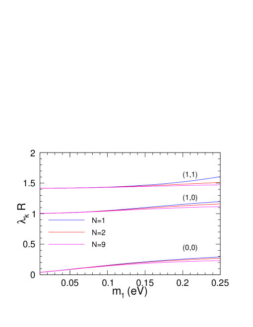
Figure 1: The figure shows the plots of $\lambda_{k}R$ as a function of $m_{1}$ for $\theta=\pi/2$ and for a fixed value of $R=3.1\times 10^{-7}$ m. Here, $k$ refers to the $k^{th}$ eigen value corresponding to a given $(m,n)$ mode. The eigen value $\lambda_{k}$ is defined as $\frac{1}{3}\sum_{j}\lambda_{k}^{j}$.

The fig. 1 shows the plot of eigen values $\lambda_{k}R$ as a function of mass $m_{1}$ for $N=1,2,9$ (other masses are fixed based on NH) solved iteratively using the Eq. 21. The eigen value $\lambda_{k}$ is defined as the average $\frac{1}{3}\sum_{j}\lambda_{k}^{j}$. It is easy to check that Eq. 21 has large number of solutions $\lambda_{k}$ depending on the $m$ , $n$ and $N$ values, although shown for only $(0,0)$, $(1,0)$ and $(1,1)$ modes only since $(0,1)$ and $(1,0)$ modes are degenerate. As can be seen, the solutions are not convergent due to logarithmic divergent and strongly depend on the choice of cut-off value $N$ particularly for large $m_{1}$ values. However, for small $m_{1}$ (more specifically when $\xi_{j}=m_{\nu}^{j}R<<1$), the dependency on $N$ is rather weak and the solutions for $m$ or $n$ $\geq 1$, can be approximated by Dienes ; Cao ,

$$\lambda_{k}=\frac{k_{mn}}{R}\big{(}1+\frac{\xi^{2}_{j}}{k_{mn}^{2}}-\frac{\xi^{4}_{j}}{k_{mn}^{4}}+....\big{)}.$$ (26)

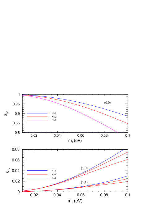
Figure 2: The top panel shows the plots of $S_{\alpha 0}$ for $(0,0)$ mode as the function of $m_{1}$ for $N=1$, $N=2$ and $N=9$ respectively. The bottom panel shows the similar plots for $(1,0)$ and $(1,1)$ modes. The parameters used are same as that of fig. 1.

The top panel of fig. 2 shows the plots of $S^{\alpha 0}$ as given in Eq. 25 as the function of $m_{1}$ for $N=1$, $N=2$ and $N=9$ respectively for $(0,0)$ mode. It is noticed that $S_{\alpha 0}$ is close to unity when $m_{1}$ is very small as expected, however unitarity is violated with increasing $m_{1}$. The unitarity is violated by more than $5\%$ at $m_{1}=0.05$ eV even when $N=2$. The bottom pannel shows the similar plots for $(1,0)$ and $(1,1)$ modes respectively. As can be seen, the value of $S_{\alpha k}$ strongly depends on $N$ at large values of $m_{1}$ even though $S_{\alpha 0}$ starts decreasing significantly with increasing $N$. Since $S_{\alpha k}$ is not very sensitive to $N$ for small mass, the mixing probability $(L_{j}^{0k})^{2}$ (hence $S_{\alpha k}$) can be approximated by,

$$(L_{j}^{0k})^{2}=\frac{2d_{k}\xi_{j}^{2}}{k_{mn}^{2}}.$$ (27)

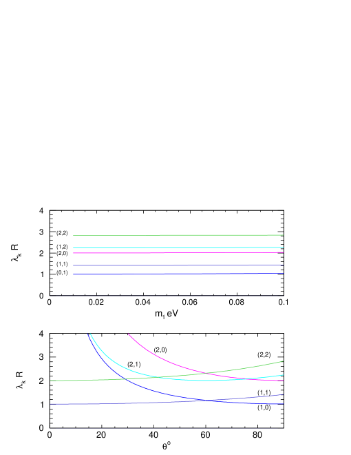
Figure 3: The top panel shows the plots of $\lambda_{k}R$ as a function of $m_{1}$ for $(1,0)$, $(1,1)$, $(2,0)$, $(2,1)$ and $(2,2)$ modes corresponding to $N=2$, $\theta=\pi/2$ and $R=3.1\times 10^{-7}$. The bottom panel shows the similar plots as a function of $\theta$ at a fixed mass $m_{1}=0.052$ eV.

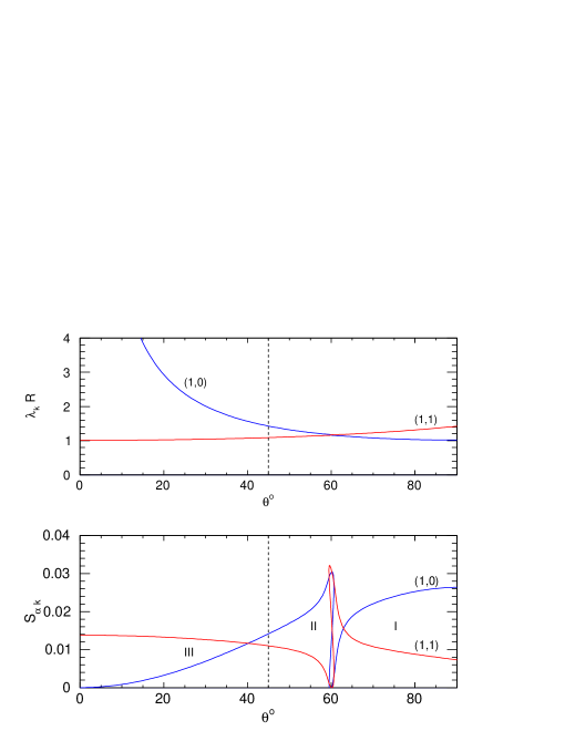
Figure 4: The top panel shows the plot of $\lambda_{k}R$ as a function of $\theta$ for $(1,0)$ and $(1,1)$ modes. The other parameters are $N=1$, $m_{1}=0.052$ eV and $R=3.1\times 10^{-7}$ m. The bottom panel shows the corrresponding $S_{\alpha k}$ as a function of $\theta$.

The top panel of fig. 3 shows the plot of $\lambda_{k}R$ as a function of $m_{1}$ for a few lowest mass states corresponding to $N=2$. This corresponds to the case of normal torus for which $\theta=\pi/2$. The other parameter values are listed in the figure caption. For small values of $m_{1}$, $\lambda_{k}R$ is nearly equal to $k_{mn}$ as expected. The ratio of the mass gaps with respect to the lowest one are $\sqrt{2}$, $2$, $\sqrt{5}$, $2\sqrt{2}$ respectively. The bottom panel shows the similar plot but as a function of $\theta$ at a fixed mass $m_{1}=0.52$ eV. The pattern of KK mass gaps now change with decreasing $\theta$ and exhibit level crossing making some of the higher modes lighter as compared to lower ones. Although this phenomena has been studied in detail before Dienes_prl1 ; Dienes_prl2 , we consider here only the first two mass states $(1,0)$ and $(1,1)$ which shows level crossing for $\theta<\pi/3$ which is shown more specifically in fig. 4 (see top panel). The bottom panel shows the active-sterile mixing probabilities $S_{\alpha 1}$ and $S_{\alpha 2}$ as a function of $\theta$. In the region I, mass of $(1,1)$ mode is higer than $(1,0)$ mode and in the region III, the mass of $(1,0)$ mode is higher than $(1,1)$ mode. Accordinly, the mixing probability $S_{\alpha 1}>S_{\alpha 2}$ in region I and $S_{\alpha 2}>S_{\alpha 1}$ in region III as expected. However, the behavior is different in region II where $S_{\alpha 1}>S_{\alpha 2}$ even though the mass of $(1,0)$ mode is heavier than the mass of $(1,1)$ mode which is contrary to the naive expectation. For $\theta<60^{o}$, although the mass of $(0,1)$ mode becomes higher than the mass of $(1,1)$ mode, the $(0,1)$ mode has degeneracy two times higher than $(1,1)$ mode. So the net result is $S_{\alpha 1}$ remains higher than $S_{\alpha 2}$ for small values of $\xi$ (see Eq. 27). It can be seen that at around $\theta\sim 40^{o}$, the two mixing probabilities are nearly equal as the mass of $(1,0)$ mode is nearly $\sqrt{2}$ times higher than mass of $(1,0)$ mode. In general, $S_{\alpha 1}\geq S_{\alpha 2}$ in the range $40^{o}<\theta<60^{o}$. Associating the mass of $(1,0)$ mode to $\Delta m_{15}$ and mass of $(1,1)$ mode to $\Delta m_{14}$ in the region II, it would mean $|U_{e5}|\geq|U_{e4}|$. This is an interesting observation indicating that there exists a range in $\theta$ where the mixing probability may become higher for havier mass and can be verified experimentally. In the present study, we have three parameters $m_{1}$, $R$ and $\theta$. While $R$ decides the mass scale, $m_{1}$ controls the mixing probability and the angle $\theta$ decides the relative strength of the active-sterile coupling strength. Although, we do not optimize the above parameters to explain experimental observations, we notice that the choice of $R\sim 3.1\times 10^{-7}$ m, $m_{1}=0.052$ $eV$ and $\theta=\pi/4$ describes the experimental observations reasonably well.

Table 1: The extracted parameters using $m_{1}=0.052$ eV and $R=0.31\times 10^{-7}$ $m$ both for NH and IH.

Type	Angle	$\Delta m_{14}^{2}~{}(eV^{2})$	$\Delta m_{15}^{2}~{}(eV^{2})$	$|U_{e4}|$	$|U_{e5}|$
NH	$90^{o}$	0.42	0.82	0.160	0.09
IH	$90^{o}$	0.42	0.81	0.220	0.12
NH	$45^{o}$	0.48	0.82	0.105	0.120
IH	$45^{o}$	0.48	0.83	0.137	0.160

Table 2: The $(3+2)$ global fit parameters taken from [7]. The values in first row are extracted from reactor anti-neutrino data and the values in second row are exracted from global fits.

$\Delta m_{14}^{2}~{}(eV^{2})$	$\Delta m_{15}^{2}~{}(eV^{2})$	$|U_{e4}|$	$|U_{e5}|$
0.46	0.89	0.108	0.124
0.47	0.87	0.128	0.138

In table 1, we have listed a few parameters estimated at $\theta=\pi/4$ and $\theta=\pi/2$ using both normal and inverted hierachy. The estimated values are compared with the reported results which are given in the table 2. The choice of $m_{1}=0.052$ $eV$ results in total active neutrino mass $\sum m_{\nu}=0.176$ eV which is less than the latest cosmological bound $\sum m_{\nu}<0.183$ $eV$ Giu . Since inclusion of sterile neutrino will exceed this upper bound, probably sterile neutrinos if present are not in thermal equilibrium in the cosmological context.

IV Fourier transform of reactor anti-neutrino spectra

The reactor anti-neutrino flux can be parametrized as the exponential of a fifth order polynomial valid in the range $1.8\leq E\leq 8$ MeV huber ; muller ,

$$\Phi(E)=exp\left(\sum_{i=1}^{6}\alpha_{i}E^{i-1}\right),$$ (28)

where $\alpha_{i}$s are listed in table 3.

Table 3: The fit parameters for various isotopes that contribute to the total power of the reactor. The parameters except for $U^{238}$ are taken from huber and for $U^{238}$ from muller .

	Isotope	$~{}~{}\alpha_{0}$	$\alpha_{1}$	$\alpha_{2}$	$\alpha_{3}$	$\alpha_{4}$	$\alpha_{5}$
	$U^{235}$	4.367	-4.577	2.100	-5.294(-1)	6.186(-2)	-2.777(-3)
	$U^{238}$	4.833(-1)	1.927(-1)	-1.283(-1)	-6.762(-3)	2.233(-3)	-1.536(-4)
	$Pu^{239}$	4.757	-5.392	2.563	-6.596(-1)	7.820(-2)	-3.536(-3)
	$Pu^{241}$	2.990	-2.882	1.278	-3.343(-1)	3.905(-2)	-1.754(-3)

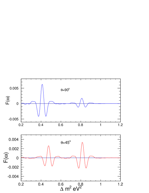
Figure 5: The plot of the cosine Fourier transform (in arbitrary unit) as a function of $\Delta m^{2}$ at $\theta=\pi/2$ and $\theta=\pi/4$. The other parameters are as that of fig 4.

The differential yield at energy $E$ and distance $L$ can be written as,

$$Y(L,E)=\Phi(E)\sigma(E)P_{ee}(L,E),$$ (29)

where $E$ is the energy of reactor anti-neutrino, $\sigma(E)$ is the interaction cross section of anti-neutrino with matter and $P_{e,e}$ is the anti-neutrino survival probability as defined in Eq. 24. The leading order expression for the cross section of inverse-$\beta$ decay ($\bar{\nu}_{e}\rightarrow e^{+}+n$) is given by Vogel ,

$$\sigma=0.0952\times 10^{-42}~{}cm^{2}~{}(E_{e}p_{e}/~{}1MeV^{2}).$$ (30)

where $E_{e}=E_{\bar{\nu}}-(M_{n}-M_{p})$ is the positron energy when neutron recoil energy is ignored and $p_{e}$ is the positron momentum. The fractional contributions of $U^{235}:U^{238}:Pu^{239}:Pu^{241}$ to the total power are taken in the ratio $0.538:0.078:0.328:0.056$ respectively. We consider two sterile mass states corresponding to the parameters $m_{1}=0.052$ eV and $R=3.1\times 10^{-7}$ m. This corresponds to $\Delta m_{14}^{2}\sim 0.42$ $eV^{2}$, $\Delta_{15}^{2}\sim 0.82$ $eV^{2}$ when $\theta=\pi/2$ and $\Delta m_{14}^{2}\sim 0.48$ $eV^{2}$ , $\Delta_{15}^{2}\sim 0.82$ $eV^{2}$ when $\theta=\pi/4$ (see table 1). In order to locate the mass peak, we consider the fourier cosine transform in the $1/E$ space given by Zhan ,

$$F(\omega,L)=\int_{t_{min}}^{t_{max}}\big{[}Y(L,t)-Y_{0}(E,L)\big{]}cos(\omega t)dt,$$ (31)

where $t=1/E$ which varies from $1/E_{max}$ to $1/E_{min}$ ($E_{max}=8$ MeV and $E_{min}=1.8$ MeV) and $\omega$ plays the role of frequency but in units of eV. We define $Y_{0}(E,L)$ as the yield without $P_{ee}$ term in Eq. 24. We have introduced $Y_{0}$ in Eq. 31 to improve the sensitivity by substracting a background term. The fig. 5 shows the cosine Fourier transform of the above spectrum as a function of $\Delta m^{2}=\omega/(2.54L)$ which shows sharp peaks when $\omega~{}\sim 2.54L\Delta m^{2}$. Since the active neutrino masses are nearly degenerate as compared to the sterile masses, the peaks appear at $\lambda_{mn}^{2}/R^{2}$. When $\theta=\pi/2$, the two lowest modes are $(1,0)$ and $(1,1)$ corresponding to mass square difference of $0.42$ $eV^{2}$ and $0.82$ $eV^{2}$ respectively as shown in top panel. Although $F(\omega)$ is shown in arbitray units, the height is proportional to the mixing probability. Since the height of first peak is more than the second, it would mean $|U_{14}|>|U_{15}|$. The bottom panel shows the plot when $\theta=\pi/4$ corresponding to mass square differences of $0.48$ $eV^{2}$ and $0.82$ $eV^{2}$ respectively. In this case, the height of the second peak is more than the first one resulting $|U_{15}|>|U_{14}|$. Although shown for $\theta=\pi/4$, it is noticed that in general $|U_{15}|\geq|U_{14}|$ in the theta range $40^{o}<\theta<60^{0}$ even though $\Delta m_{15}^{2}>\Delta m_{14}^{2}$.

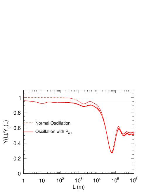
Figure 6: The plot of the ratio of $Y(L)/Y_{0}(L)$ as a function of $L$. The dotted curve is obtained using normal oscillation parameters i.e. the probability $P_{ee}$ is obtained without using $L^{0k}$ factor. The solid curve is obtained using $P_{ee}$ with $L^{0k}$ included. This plot corresponds to $\theta=45^{o}$, $R=3.1\times 10^{-7}$, $m_{1}=0.052$ eV with normal hierarchy. The line represents the average value at $0.94$.

Figure 6 shows the ratio of the total yield $Y(L)/Y_{0}(L)$ as a function of $L$ in $m$. The dotted curve is obtained using normal oscillation probability $P_{ee}$ which does not include the active-sterile oscillation factor $L^{0k}$.

The anti-neutrino survival probability is lowest when the argument in the exponential of Eq. 24 is $\pi$. This corresponds to the relation,

$$L\sim\frac{1.2E}{\Delta m^{2}},$$ (32)

.

where we have replaced $\lambda^{2}$ by $\Delta m^{2}$. For normal oscillation, the dips occur at $L\sim 2000$ m and $L\sim 60000$ m corresponding to $\Delta m_{13}^{2}=2.42\times 10^{-3}$ $eV^{2}$ and $\Delta m_{12}^{2}=7.45\times 10^{-5}$ $eV^{2}$ respectively. This is consistent with the relation given by Eq. 32 if we cnsider $<E>\sim 4$ MeV. When $L^{0k}$ is included, another dip occurs at $L\sim 10$ m corresponding to $\Delta m^{2}=0.48$ $eV^{2}$. The effect due to other higher masses are not significant as the mixing probability decrerases with increasing mass. The black dotted line indicates the ratio at $0.94$ which is the average deficit reported in Muller.

V Conclusions

We have considered a toroidal extra dimensional space associated with a shape moduli characterized by an angle $\theta$ between the two large extra dimensions $R_{1}$ and $R_{2}$. The Kaluza-Klein compactification results in a tower of bulk neutrinos which couple to the active neutrinos at the brane. The active-sterile mixing probability depends strongly on the angle $\theta$ due to changing pattern of KK mas gaps resulting in level crossing. Considering only the first two KK mass states corresponding to $(1,0)$ and $(1,1)$ modes in analogy with $(3+2)$ neutrino mixing model, it is shown that there exists a range in $\theta$ $(\sim 40^{o}<\theta<\sim 60^{o})$ where the mass of the higher $(1,1)$ KK mode is lower as compared to the mass of the $(1,0)$ or $(0,1)$ mode. Since the $(0,1)$ and $(1,0)$ modes are degerate, it results in a higher active-sterile mixing probability for $(1,0)$ mode as compared to the $(1,1)$ mode. In $(3+2)$ analogy, this would mean $|U|_{e5}>|U_{e4}|$ even though $\Delta_{15}^{2}>\Delta_{14}^{2}$. This is an important observation which can be verified from the short base line neutrino measurements, although present global anlysis seems to support the above observation at $\theta\sim\pi/4$. The fourier analysis of the reactor anti-neutrino spectra at SBL also shows more qualitatively the above features which may also be possible to verify in near future with precision measurements.

References

• (1) K. R. Dienes, Phys. Rev. Lett. 88, 011601 (2001).
• (2) K. R. Dienes and A. Mafi, Phys. Rev. Lett. 88, 011602 (2002).
• (3) N. Arkani-Hamed, S. Dimopoulos and G. R. Dvali, Phys. Lett B 429, 263 (1998).
• (4) N. Arkani-Hamed, S. Dimopoulos and G. R. Dvali, Phys. Rev. D 59, 086003 (1999).
• (5) Th. A. Muller et al, Phys. ReV. C 83, 054615, (2011).
• (6) P. Huber, Phys. ReV. C 84, 024617 (2011).
• (7) J. Kopp, M. Maltoni and T. Schwetz, Phys. Rev. Lett. 107, 091801 (2011).
• (8) J. Kopp, P. A. N. Machado, M. Maltoni and T. Schwetz, J. High Energy Physics 05, 0501 (2013).
• (9) I. Antoniadis, N. Akrani-Hamed, S. Dimopoulous and G. R. Dvali, Phys. Lett. B 436, 257 (1998).
• (10) N. Arkani-Hamed, S. Dimopoulos, G. R. Dvali and J. March-Russell, Phys. Rev. D 65, 024032 (2002).
• (11) K. R. Dienes, E. Dudas and T. Gherghetta, Nucl. Phys. B 557, 25 (1999).
• (12) G. R. Dvali and A. Y. Smirnov, Nucl. Phys. B 563, 63 (1999).
• (13) R. Barbieri, P. Creminelli and A. Strumia, Nucl. Phys. B 585, 28 (2000).
• (14) H. Davoudiasl, P. Langakker and M. Perelstein, Phy. Rev. D 65, 105015 (2002).
• (15) D. M. Gingrich, Int. Journal of Moder Physics A 24, 5173 (2009).
• (16) Q. Cao, S. Gopalakrishna and C. P. Yuan, Phys. ReV. D 69, 115003 (2004).
• (17) V. S. Basto-Gonzalez, A. Esmaili and O. L. G. Peres, Phys. Lett B 718, 1020 (2013).
• (18) W. Rodejohann and H. Zang, Phys. Lett. B 737, 81 (2014).
• (19) E. Dudas, C. Grojean and S. K. Vempati, hep-ph/051100 (2005).
• (20) M. Gonzalez-Garcia, M. maltoni, J. Salvao, T. Schwetz, J. High Energy Physics 1212 123 (2012).
• (21) A. Esmaili, O. L. G. Peres and Z. Tabrizi, J. Cosmologyand astroparticle Physics 12 002 (2014).
• (22) P. Vogel and J. F. Beacom, Phy. Rev. D60, 053003 (1999), hep-ph/9903554.
• (23) L. Zhan, Y. Wang, J. Cao and L. Wen, Phys. Rev. D78, 111103 (2008), hep-ex/0807.3203.
• (24) E. Giusarma, M. Gerbino, O. Mena, S. Vagnozzi, S. Ho and K. Freese, astro-phi/1605.04320.