Dynamical optical flow of saliency maps for predicting visual attention

Abstract

Saliency maps are used to understand human attention and visual fixation. However, while very well established for static images, there is no general agreement on how to compute a saliency map of dynamic scenes. In this paper we propose a mathematically rigorous approach to this problem, including static saliency maps of each video frame for the calculation of the optical flow. Taking into account static saliency maps for calculating the optical flow allows for overcoming the aperture problem. Our approach is able to explain human fixation behavior in situations which pose challenges to standard approaches, such as when a fixated object disappears behind an occlusion and reappears after several frames. In addition, we quantitatively compare our model against alternative solutions using a large eye tracking data set. Together, our results suggest that assessing optical flow information across a series of saliency maps gives a highly accurate and useful account of human overt attention in dynamic scenes.

1 Introduction

Humans and other primates focus their perceptual and cognitive processing on aspects of the visual input. This selectivity is known as visual attention and it is closely linked to eye movements: humans rapidly shift their center of gaze multiple times per second from one location of an image to another. These gaze shifts are called saccades, and they are necessary because high acuity vision is limited to a small central area of the visual field. Fixations are the periods between two saccades, in which the eyes rest relatively still on one location from which information is perceived with high acuity. Consequently, fixations reflect which areas of an image attract the viewer’s attention.

Models of visual attention and eye behavior can be roughly categorized into two classes: bottom-up models, which are task-independent and driven mainly by the intrinsic features of the visual stimuli, and top-down models, which are task-dependent and driven by high-level processes [1]. Our focus in this article is on bottom-up models. A central concept in bottom-up models of attention is the saliency map, which is a topographical representation of the original image representing the probability of each location to attract the viewer’s attention. Saliency maps are useful for testing hypotheses on the importance of the current image’s low-level visual features (such as color, luminance, or orientation). Moreover, saliency models allow for general predictions on the locations that are fixated by human viewers. This is important in many contexts, such as the optimization of video compression algorithms or of graphical user interfaces at the workplace as well as in entertainment environments, to name but a few examples. A location in an image is considered salient if it stands out compared to its local surroundings.

Saliency maps are often computed based on low-level visual features and their local contrast strengths in dimensions such as color, luminance, or orientation. A well-known model for static scenes is the one of [2]. Other examples are graph-based visual saliency (GBVS)[3], gaze-attentive fixation finding engine (GAFFE)[4], frequency-tuned saliency detection model [5] and models based on phase spectrum, explained by the inverse Fourier transform [6].

Recent work is devoted to develop concepts of saliency maps of dynamic sequences [7, 8, 9, 10, 11, 12]. These spatial-temporal saliency maps are modeled as the weighted sum of motion features and of static saliency maps [7, 9, 8, 10, 13, 11, 14, 15, 16, 12, 17, 18].

The present work introduces a novel dynamic saliency map, which is the optical flow of a high-dimensional dynamic sequence. Extending the concept of saliency to dynamic sequences by including optical flow as an additional source for bottom-up saliency is not new per se [19, 15, 20, 21]. However, while other researchers use the optical flow as a feature of the dynamic saliency map, we define the dynamic saliency map as the optical flow itself. In detail:

1. we calculate the flow of a virtual, high-dimensional image sequence, which consists of (i) intensity and (ii) color channels, complemented by saliency maps, respectively;

2. we also consider the complete movie (consisting of all frames) for the computation of a dynamic saliency map. In contrast, in [7, 9, 8, 10, 13, 11, 14, 15, 16, 12, 17, 18] (as it is standard), dynamic saliency maps are obtained from optical flow features (see Figure 1) of two consecutive frames. As we show below in section 4 this can lead to misinterpretations of visual attention, for instance, in the case of occlusions.

Figure 1: The standard approach for calculating a dynamic saliency map

Our algorithm for calculating the dynamic saliency map is schematically depicted in Figure 2.

Figure 2: The proposed approach for calculating a dynamic saliency map.

From the different methods proposed in the literature to estimate optical flow, we focus on variational methods, which are key methods in computational image processing and computer vision.

The outline of this paper is as follows: in section 2 we review the optical flow, introduce the new model and derive a fixed-point algorithm for the computational realization; in section 3 we discuss the acquisition of the eye tracking data; finally, in sections 4 and 5 we present experiments, results and a discussion.

2 Computational methods

The optical flow denotes the pattern of apparent motion of objects and surfaces in a dynamic sequence. The computational model of optical flow is based on the brightness-constancy assumption, requiring that for every pixel there exists a path through the movie which conserves brightness.

2.1 Basic optical flow calculations

We briefly outline the concept in a continuous mathematical formulation. We consider a movie to be a time continuous recording of images, where each image is described by a function defined for $x=(x_{1},x_{2})^{t}$ in the Euclidean plane $\mathbbm{R}^{2}$. This function representing the image is called frame. Moreover, we assume that the movie to be analyzed has unit-length in time. That is, the movie can be parametrized by a time $t\in[0,1]$. If the frames composing a movie consist of gray-valued images, then we describe each by a function $f:\mathbbm{R}^{2}\to\mathbbm{R}$. If the frame is completed by a spatial saliency map, then $\vec{f}:=(f_{1};f_{2})^{t}:\mathbbm{R}^{2}\to\mathbbm{R}^{2}$, where $f_{1}$ is the recorded movie and $f_{2}$ is the according saliency map. For a color frame, $\vec{f}:=(f_{1},f_{2},f_{3})^{t}:\mathbbm{R}^{2}\to\mathbbm{R}^{3}$, where each component represents a channel of the color images; typically RGB (red-green-blue) or HSV (hue-saturation-value) channels. A color frame, which is complemented by a saliency map is described by $\vec{f}:=(f_{1},f_{2},f_{3};f_{4})^{t}:\mathbbm{R}^{2}\to\mathbbm{R}^{4}$, where the first three components are the color channels and the fourth component is the according saliency map. For the sake of simplicity of notation, from now on, we will always write $\vec{f}$, even if $f$ is a gray-valued image.

The optical flow equation is derived from the brightness constancy assumption, which considers paths $\gamma$ of constant intensity of the movie or the saliency complemented movie, respectively. Note that in our setting we consider brightness in each component. That is for

$$\vec{f}(\gamma(x,t),t)=\vec{c}$$ (1)

for some constant vector $\vec{c}$. Note that we do not differentiate in our notation between intensity, color, or saliency completed movies anymore and always write $\vec{f}$ for the image data.

A differential formulation of the brightness constancy assumption follows from (1) by differentiation with respect to time (see for instance [22]):

$$J_{\vec{f}\,}(x,t)\cdot\vec{u}(x,t)+\frac{d\vec{f}}{dt}(x,t)=0\text{ for all }x\in\mathbbm{R}^{2}\text{ and }t\in(0,1)\,,$$ (2)

where $\vec{u}(x,t)=(u_{1}(x,t),u_{2}(x,t))=\frac{d\gamma}{dt}(x,t)$ is the optical flow and $J_{\vec{f}\,},\frac{d\vec{f}}{dt}$ are the partial derivatives in space and time of the function $\vec{f}$, respectively. Note that $(u_{1}(x,t),u_{2}(x,t))$ can both be vectors, and that the Jacobian $J_{\vec{f}\,}=\nabla\vec{f}=\left(\frac{\partial}{\partial x_{1}}\vec{f},\frac{\partial}{\partial x_{2}}\vec{f}\,\right)$ is a two-dimensional vector if the movie is gray-valued, a $(2\times 2)$-dimensional matrix if it is a saliency complemented gray-valued image, a $(3\times 2)$-dimensional matrix if it is in color, and a $(4\times 2)$-dimensional matrix if a color image is complemented by a saliency map.

Equation (2) is uniquely solvable at points $(x,t)$ where $J_{\vec{f}\,}$ has full-rank $2$. For gray-valued movies the matrix can have at most rank of one, and thus the two unknown functions $u_{1}$ and $u_{2}$ cannot be reconstructed uniquely from this equation. This is known as the aperture problem in Computer Vision. The non-uniqueness is taken care of mathematically by restricting attention to the minimum energy solution of (2) which minimizes, among all solutions, an appropriately chosen energy, such as the one proposed in [22]:

$$\mathcal{E}[t](\vec{u}):=\int_{\mathbbm{R}^{2}}|\nabla u_{1}(x,t)|^{2}+|\nabla u_{2}(x,t)|^{2}dx\text{ for all }t\in[0,1].$$ (3)

For every $t\in(0,1)$ the minimum energy solution can be approximated (see for instance [23] for a rigorous mathematical statement) by the minimizer of

$$\mathcal{F}[t](\vec{u}):= \int_{\mathbbm{R}^{2}}\left|J_{\vec{f}\,}(x,t)\cdot\vec{u}(x,t)+\frac{d\vec{f}}{dt}(x,t)\right|^{2}dx$$ (4)

$$+\alpha\int_{\mathbbm{R}^{2}}|\nabla u_{1}(x,t)|^{2}+|\nabla u_{2}(x,t)|^{2}dx.$$

Here $\alpha>0$ is a weight (also called regularization) parameter.

Different optical flow methods have been considered in the literature, which are formulated via different regularization energies. For instance, in [24] it was suggested to minimize

$$\int_{\mathbbm{R}^{2}}\left|J_{\vec{f}\,}(x,t)\cdot\vec{u}(x,t)+\frac{d\vec{f}}{dt}(x,t)\right|^{2} +\alpha\Psi(|\nabla u_{1}(x,t)|^{2}+|\nabla u_{2}(x,t)|^{2})dx$$ (5)

$$\text{ for all }t\in[0,1],$$

where $\Psi:\mathbbm{R}_{0}^{+}\rightarrow\mathbbm{R}_{0}^{+}$ is a monotonically increasing, differentiable function. Note that in the original work of [24] the function $\vec{f}$ is not saliency complemented and the data $\vec{f}$ only represents intensity images.

We note that in most applications, $\mathcal{F}[t]$ is realized by replacing $J_{\vec{f}\,}$ by the spatial difference quotients, $\frac{d\vec{f}}{dt}$ by the temporal difference of two consecutive frames $\vec{f}{(x,t_{i})}$, $i=1,2$, respectively, and appropriate scaling. This results in the functional to be minimized:

$$\int_{\mathbbm{R}^{2}}\left|J_{{\vec{f}(\cdot,t_{1})\,}}(x)\cdot\vec{u}(x)+\vec{f}(x,t_{2})-\vec{f}(x,t_{1})\right|^{2}dx$$ (6)

$$+\alpha\int_{\mathbbm{R}^{2}}\Psi(|\nabla u_{1}(x)|^{2}+|\nabla u_{2}(x)|^{2})dx.$$

Remark 1

We emphasize that by the approximation of $\frac{d\vec{f}}{dt}$ with the finite difference $\vec{f}(x,t_{2})-\vec{f}(x,t_{1})$ (where, we assume that after time scaling we have $t_{2}-t_{1}=1$), the equations (2) and

$$J_{\vec{f}(\cdot,t_{1})\,}(x)\cdot\vec{u}(x)+\vec{f}(x,t_{2})-\vec{f}(x,t_{1})=0\text{ for all }x\in\mathbbm{R}^{2}\,,$$ (7)

might not be correlated anymore. This is especially true for large displacements $\gamma-I$. In order to overcome this discrepancy, researchers in computer vision proposed to use computational coarse-to-fine strategies [25, 26, 27, 28, 29, 30].

We emphasize that in all these approaches the temporal coherence of the movie is neglected and this can lead to rather abruptly changing flow sequences. Therefore, in [24], a spatial-temporal regularization was suggested, which consists in minimization of

$$\int_{\mathbbm{R}^{2}\times[0,1]}\left|J_{\vec{f}\,}(x,t)\cdot\vec{u}(x,t)+\frac{d\vec{f}}{dt}(x,t)\right|^{2}+\alpha\Psi(|\nabla_{3}u_{1}(x,t)|^{2}+|\nabla_{3}u_{2}(x,t)|^{2})dxdt,$$ (8)

where $\nabla_{3}=(\nabla,\frac{\partial}{\partial t})$ denotes the spatial-temporal gradient operator. More sophisticated spatial-temporal regularization approaches have been proposed in [31, 32, 33, 34, 35, 24].

2.2 Spatial saliency for optical flow computations

In the following section we investigate the effect of complementing intensity and color images with a spatial saliency map on optical flow computations. We use the GBVS method, introduced by [3], which defines a spatial saliency for each frame. Note however, that our approach is not restricted to this particular choice.

We verify the hypothesis that the complemented data uniquely determines the optical flow in selected regions - that is, where $J_{\vec{f}}$ has full rank. A conceptually similar strategy was implemented in [15] where the image data was complemented by Gabor filters as input of (2). Here, we verify this thesis by checking the spatially dependent condition number of $J_{\vec{f}}$ in the plane, and by tabbing the area of the points in a region where the condition number is below 1000 (see Table 1). In these regions we expect that the flow can be computed accurately from (2) without any regularization. We recall that for gray-valued images the optical flow equation is under-determined and the matrix $J_{\vec{f}}$ is singular, or in other words, the condition number is infinite. However, if the intensity data is complemented by a saliency map, $3\text{ to }17\%$ of the pixels have a condition number smaller than 1000, such that the solution of (2) can be determined in a numerically stable way. For color images the optical flow equation is already over-determined and $1\text{ to }5\%$ of the pixels have a small condition number. However, if the color information is complemented by a saliency information, $3\text{ to }33\%$ of the pixels have this feature. These results suggest that complementing the original information by saliency is useful for accurate computations of the optical flow.

Sequence	Saliency-Brightness	Saliency-Color	Color
Backyard	3.16%	8.18%	2.45%
Basketball	3.68%	10.06%	1.26%
Beanbags	4.07%	9.73%	0.9%
Dimetrodon	5.91%	7.54%	1.07%
DogDance	3.99%	9.57%	2.50%
Dumptruck	5.20%	10.13%	3.35%
Evergreen	6.12%	12.48%	3.20%
Grove	12.61%	18.94%	4.86%
Grove2	15.48%	24.07%	3.29%
Grove3	16.49%	25.27%	4.20%
Hydrangea	10.30%	29.93%	2.48%
Mequon	11.44%	19.12%	2.38%
MiniCooper	7.35%	16.77%	3.76%
RubberWhale	8.45%	22.34%	1.46%
Schefflera	12.12%	20.02%	1.98%
Teddy	16.65%	32.96%	4.63%
Urban2	3.17%	3.35%	0.31%
Venus	12.86%	17.84%	2.75%
Walking	2.85%	7.41%	1.25%
Wooden	3.38%	7.76%	0.75%

Table 1: Percentage of the pixels with condition number smaller than 1000 for different sequences from the Middleburry Dataset [36]. For each sequence we use the third frame and its spatial saliency as input.

2.3 Contrast invariance

We also aim to recognize motion under varying illumination conditions because humans have this visual capacity. However, a typical optical flow model, like the one in (8), would not yield contrast invariant optical flow although this would be necessary for motion recognition under varying illumination conditions.

In order to restore contrast invariance for the minimizer of the optical flow functional, as proposed (for a different reason) by [37] and by [38, 39], we introduce the semi-norm $\|\cdot\|_{\mathcal{B}}^{2}$ like:

$$\|w\|_{\mathcal{B}}^{2}=w^{T}\text{diag}(b_{1},...,b_{n})w\,,$$

where $b_{i}$ are the components of a vector $\mathcal{B}$. For gray-valued images complemented with saliency $\vec{f}=(f_{1};f_{2})$ the vector $\mathcal{B}$ is defined as:

$$\mathcal{B}=\begin{pmatrix}\frac{f_{2}}{\sqrt{|\nabla f_{1}|^{2}+\xi^{2}}},1\end{pmatrix}.$$ (9)

For saliency complemented color images $\vec{f}=(f_{1},f_{2},f_{3};f_{4})$ we define

$$\mathcal{B}=\begin{pmatrix}\frac{f_{4}}{\sqrt{|\nabla f_{1}|^{2}}},\frac{f_{4}}{\sqrt{|\nabla f_{2}|^{2}+\xi^{2}}},\frac{f_{4}}{\sqrt{|\nabla f_{3}|^{2}+\xi^{2}}},1\end{pmatrix}.$$ (10)

The vectors $\mathcal{B}$ are the product of the weighting factors $\frac{1}{\sqrt{|\nabla f_{i}|^{2}+\xi^{2}}}$ and the saliency map, respectively. This means that features with high spatial saliency will be weighted stronger, and thus more emphasis on a precise optical flow calculation is given to these regions. We are then using the weighted semi-norm as an error measure of the residual of (2):

$$\int_{\mathbbm{R}^{2}\times[0,1]}\left\|J_{\vec{f\,}}(x,t)\cdot\vec{u}(x,t)+\frac{d\vec{f}}{dt}(x,t)\right\|_{\mathcal{B}}^{2}\;.$$ (11)

Finally, one needs to choose the constant $\xi$ for the denominator of each weighting factor. As in [37] we choose $\xi=0.01$.

2.4 The final model

We use as a regularization functional

$$\int_{\mathbbm{R}^{2}\times[0,1]}\Psi(|\nabla_{3}u_{1}(x,t)|^{2}+|\nabla_{3}u_{2}(x,t)|^{2})dxdt$$

as in [24], with the difference that the function $\Psi(r^{2})=\epsilon r^{2}+(1-\epsilon)\lambda^{2}\sqrt{1+\frac{r^{2}}{\lambda^{2}}}$ is replaced by

$$\Psi(r^{2})=\sqrt{r^{2}+\epsilon^{2}}\text{ with }\epsilon=10^{-6}$$ (12)

as in [40]. Moreover, we substitute the spatial-temporal gradient operator in [24] with $\nabla_{3}=(\nabla,\lambda\frac{\partial}{\partial t})$. In numerical realizations, the weighting parameter $\lambda$ corresponds to the ratio of the sampling in space squared and the one in time The resulting model for optical flow computations then consists in minimization of the functional

$$\int_{\mathbbm{R}^{2}\times[0,1]}\left\|{J_{f}(x,t)\cdot\vec{u}(x,t)+\frac{d\vec{f}}{dt}(x,t)}\right\|_{\mathcal{B}}^{2}+\alpha\Psi(|\nabla_{3}u_{1}(x,t)|^{2}+|\nabla_{3}u_{2}(x,t)|^{2})dxdt.$$ (13)

.

2.4.1 Numerical solution

The ultimate goal is to find the path $\gamma$ solving (1), that is connecting a movie sequence. By applying Taylor expansion one sees that $\vec{u}\sim\frac{d\gamma}{dt}(x,t)t$ for small $t$. As we have stated in Remark (1), when trying to find approximations of $\gamma$ via minimization of the proposed functional (13) a coarse-to-fine strategy [25, 26, 27, 28, 29, 30] is useful for the following two reasons:

First, since at a coarse level of discretization large displacements appear relatively small, the optical flow equation (2), which is a linearization of the brightness constancy equation (1), is a good approximation of that. Indeed, a displacement of one pixel at the coarsest level of a 4-layer pyramid can represent 4 pixels of distance in the finest layer. With reference to [41], we can assume that on the coarsest level, the discretized energy functional has a unique global minimum and that the displacements are still small. We further expect to obtain the global minimum by refining the problem at finer scales and using the outcome of the coarser iteration as an initial guess of the fine level.

Second, this strategy results in a faster algorithm [36]. The optical flow is computed on the coarsest level, where the images are composed by fewest pixels, and then upsampled and used to initialize the next level. The initialization results in far lesser iterations at each level. For this reason, an algorithm using coarse-to-fine strategy tends to be significantly faster than an algorithm using only the finest level. For the coarse-to-fine strategy, we use four pyramid levels and a bicubic interpolation between each level.

In this paper, we combine the coarse-to-fine strategy with two nested fixed-point iterations. We apply a presmoothing at each level, by convolving the images with a Gaussian kernel with standard deviation one, as proposed by [42]. We solve the minimization problem on each pyramid level starting from the coarsest one. There, we initialize the optical flow $\vec{u}$ by $0$. The solution of the minimization problem is smoothed applying a median filter, as proposed in [43], and then prolonged to the next finer level. There, we employ it for the initialization of the fixed-point iterations.

For the purpose of numerical realization we call the iterates of the fixed point iteration $u_{i}^{(k)}$ for $k=1,2,...,K$ where $K$ denotes the maximal number of iterations. We plot the pseudo-code to illustrate the structure of the algorithm in Figure 3.

Given an input sequence f

Initialization

for all frame in the sequence do

     create a pyramid of 4 levels

     calculate the saliency map

     smooth the frame

end for

for each level $lev\in$ 1..4  do

     if lev=1 then

         $u_{1}^{(k)}$=0

         $u_{2}^{(k)}$=0

     else

         $u_{1}^{(k)}$= $u_{1}^{(k+1)}$

         $u_{2}^{(k)}$= $u_{2}^{(k+1)}$

     end if

     while the precision tolerance $\geq 0.001$ do

         Calculate an approximation of $u_{1}^{(k+1)}$ and $u_{2}^{(k+1)}$

         solving fixed point iterations

     end while

     Apply median filtering to the flow

     Rescale $u_{1}^{(k+1)}$ and $u_{2}^{(k+1)}$ with bicubic interpolation

end for

Figure 3: Pseudo-code to illustrate the structure of the algorithm

For each level of the pyramid we compute with the fixed point iterations the solution of the optimality condition of the functional (13):

$$0=\sum_{i=1}^{\sigma}\mathcal{B}_{i}\frac{\partial f_{i}}{\partial x_{1}}\left(\frac{\partial f_{i}}{\partial x_{1}}u_{1}+\frac{\partial f_{i}}{\partial x_{2}}u_{2}+\frac{\partial f_{i}}{\partial t}\right)-\nabla_{3}\cdot(\Psi^{\prime}(|\nabla_{3}u_{1}|^{2}+|\nabla_{3}u_{2}|^{2})\nabla_{3}u_{1})$$ (14)

$$0=\sum_{i=1}^{\sigma}\mathcal{B}_{i}\frac{\partial f_{i}}{\partial x_{2}}\left(\frac{\partial f_{i}}{\partial x_{1}}u_{1}+\frac{\partial f_{i}}{\partial x_{2}}u_{2}+\frac{\partial f_{i}}{\partial t}\right)-\nabla_{3}\cdot(\Psi^{\prime}(|\nabla_{3}u_{1}|^{2}+|\nabla_{3}u_{2}|^{2})\nabla_{3}u_{2})$$

where $\mathcal{B}_{i}$ is the i-component of the vector $\mathcal{B}$ and $\sigma=2,4$, if we consider intensity with complemented saliency data or color with complemented saliency data, respectively.

For the solution of the system of equations we use a semi-implicit Euler method: Let $\tau$ be the step size, then the fixed point iterations is defined by

$$\frac{u_{1}^{(k+1)}-u_{1}^{(k)}}{\tau} =-\sum_{i=1}^{\sigma}\mathcal{B}_{i}\frac{\partial f_{i}}{\partial x_{1}}\left(\frac{\partial f_{i}}{\partial x_{1}}u_{1}^{(k+1)}+\frac{\partial f_{i}}{\partial x_{2}}u_{2}^{(k)}+\frac{\partial f_{i}}{\partial t}\right)+$$ (15)

$$\quad\nabla_{3}\cdot(\Psi^{\prime}(|\nabla_{3}u_{1}^{(k)}|^{2}+|\nabla_{3}u_{2}^{(k)}|^{2})\nabla_{3}u_{1}^{(k)})$$

$$\frac{u_{2}^{(k+1)}-u_{2}^{(k)}}{\tau} =-\sum_{i=1}^{\sigma}\mathcal{B}_{i}\frac{\partial f_{i}}{\partial x_{2}}\left(\frac{\partial f_{i}}{\partial x_{1}}u_{1}^{(k)}+\frac{\partial f_{i}}{\partial x_{2}}u_{2}^{(k+1)}+\frac{\partial f_{i}}{\partial t}\right)$$

$$\quad+\nabla_{3}\cdot(\Psi^{\prime}(|\nabla_{3}u_{1}^{(k)}|^{2}+|\nabla_{3}u_{2}^{(k)}|^{2})\nabla_{3}u_{2}^{(k)})$$

where for the discretization of $\nabla_{3}\cdot(\Psi^{\prime}(|\nabla_{3}u_{1}^{(k)}|^{2}+|\nabla_{3}u_{2}^{(k)}|^{2})\nabla_{3}u_{1}^{(k)})$ and $\nabla_{3}\cdot(\Psi^{\prime}(|\nabla_{3}u_{1}^{(k)}|^{2}+|\nabla_{3}u_{2}^{(k)}|^{2})\nabla_{3}u_{2}^{(k)})$ we follow [24].

In our experiments we use $\tau=10^{-3}$. Moreover, we set the regularization parameter $\alpha=40$ and $\lambda=1$, unless stated otherwise. The iterations are stopped, when the Euclidean norm of the relative error

$$\frac{|u_{j}^{(k)}-u_{j}^{(k+1)}|}{|u_{j}^{(k)}|},\hskip 28.45274ptj=1,2$$

drops below the precision tolerance value of $tol=0.003$ for both the components $u_{j}$. For the discretization of (15), we use central difference approximations of $\frac{\partial f_{i}}{\partial x_{1}},\frac{\partial f_{i}}{\partial x_{2}},\frac{\partial f_{i}}{\partial t}$ for each pixel. We consider that the spacing in the central differences approximations equals a value of one with reference to space and time.

3 Eye tracking experiment

We next test our model. This is done by recording human participants’ fixations on small video clips of relatively total views of natural scenes, and testing how much of variance of fixation locations could be explained by our model as compared to two alternative models, [6] and [43]. To this end, model performances are compared using the areas under the curves (AUCs) and normalized scanpath saliency

3.0.1 Participants

Twenty-four (five female) human viewers with a mean age of 25 years (range 19–32) volunteered in an eye tracking experiment and received partial course credit in exchange. All were undergraduate Psychology students at the University of Vienna. Viewers were pre-screened for normal or fully corrected eye-sight and intact color vision. Prior to the start of the experiment, written informed consent was obtained from all participants.

3.0.2 Stimuli

The same 71 short video recordings that were used for performing the saliency computations were presented to the sample of human viewers. All videos were presented without sound. Each of the videos contained moving and potentially interesting content at several spatially distinct locations off-center (e.g., moving cars, wind moving trees, people crossing streets etc.). Hence, videos presented viewers with multiple potentially interesting fixation locations and the viewers could visually explore the scene. This distinguished the videos used here from professionally produced footage from TV shows or feature films, which often elicit strong tendencies to keep fixation at the center of the movie scene [44]. The order in which the videos were presented in the experiment was chosen randomly for each participant. All videos were presented in full screen on a CRT monitor.

3.0.3 Apparatus

Throughout each data acquisition session, the viewer’s dominant eye position was recorded using an EyeLink 1000 Desktop Mount (SR Research Ltd., Kanata, ON, Canada) video-based eye tracker sampling at 1000 Hz. The eye tracker was calibrated using a standard 9-point calibration sequence. Prior to each individual video, a fixation circle was presented at the center of the screen to perform a drift check. Whenever the acquired gaze position differed by more than $1^{\circ}$ from the fixation target’s position, the whole calibration sequence was repeated to assure maximal spatial accuracy for each viewer. Video stimuli were delivered in color to a 19-in. CRT monitor (Multiscan G400, Sony Inc.) at a screen resolution of $1280\times 1024$ pixels (85 Hz refresh rate). Viewers sat in front of the monitor and placed their head on a chin and forehead rest, which held viewing distance fixed at 64 cm, resulting in an apparent size of each full-screen video of $31\times 24.2^{\circ}$. The presentation procedure was implemented in MATLAB with the PsychToolbox and the Eyelink toolbox functions [45, 46, 47].

3.0.4 Data preprocessing

For the evaluation of the model results we compared the spatial distribution of the human viewers’ fixations on each video frame with the computed dynamic saliency maps for each frame. The recorded gaze position vector was parsed into three classes of oculomotor events: blinks, saccades, and fixations. Fixations were defined as the mean horizontal and vertical gaze position during data segments not belonging to a blink, or a saccade (gaze displacement $<0.1^{\circ}$, velocity $<30^{\circ}/s$, and acceleration $<8,000^{\circ}/s^{2}$). The parsed fixations were mapped onto each video frame depending on their start and end times. For example, if a fixation started 1.25 s after the onset the scene at location (x,y), this location was marked as fixated in a fixation matrix belonging to the 30th frame of the video. If this same fixation ended 2 s after the onset of the video, the corresponding fixation matrix from the 30th through to the 50th frame were set to true (or fixated) at that location. This mapping was done for all viewers, and all videos, resulting in a 3-dimensional fixation matrix with the spatial resolution of one video frame and the temporal extent of the number of analyzed video frames. Each video was presented for 10 s during the data collection.

4 Results

4.1 Qualitative model evaluation

This section is devoted to the evaluation of the dynamical saliency mapping by comparison with eye tracking data. High spatial saliency should correspond to active visual attention. Particular emphasis is put on the participants’ tracking of moving objects which are temporarily occluded, because this is a situation where standard optical flow algorithms fail although humans try to actively track such objects [48, 49, 50] that is, they attend to such temporarily occluded objects.

Figure 4: The dynamic sequence shows traffic in a public street. A motorcycle is riding behind a pole and it is an object of interest. We notice that when the motorcycle is occluded (central column), only (13) with saliency complemented data (top) is able to recognize the occluded part as salient. The method considering only two frames [43] (middle) does not recognize this area as salient. The method (13) without complemented data (bottom) results in a lower correlation between the saliency map and the fixation distribution.

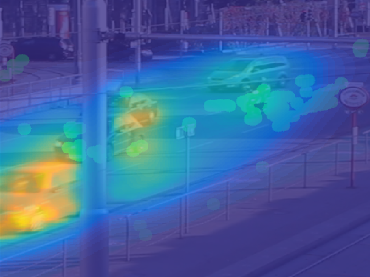
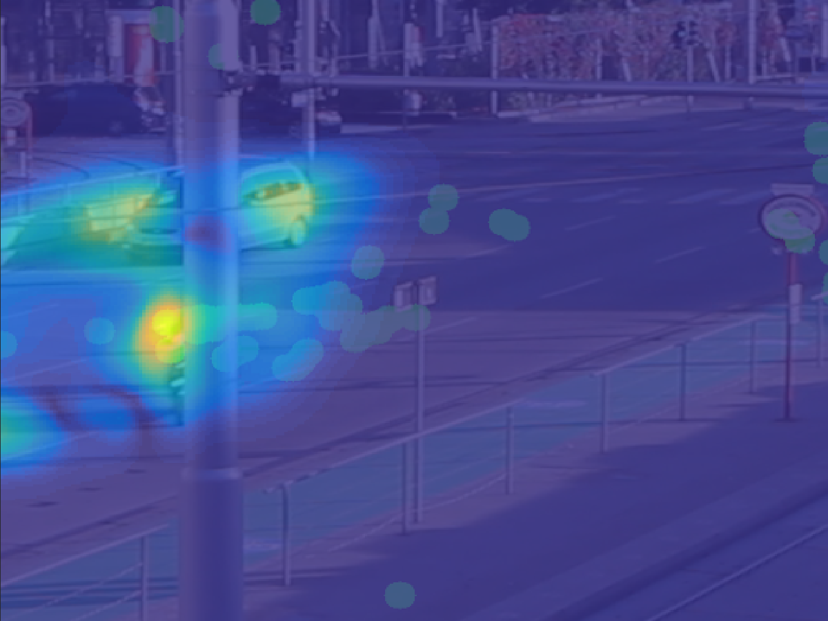
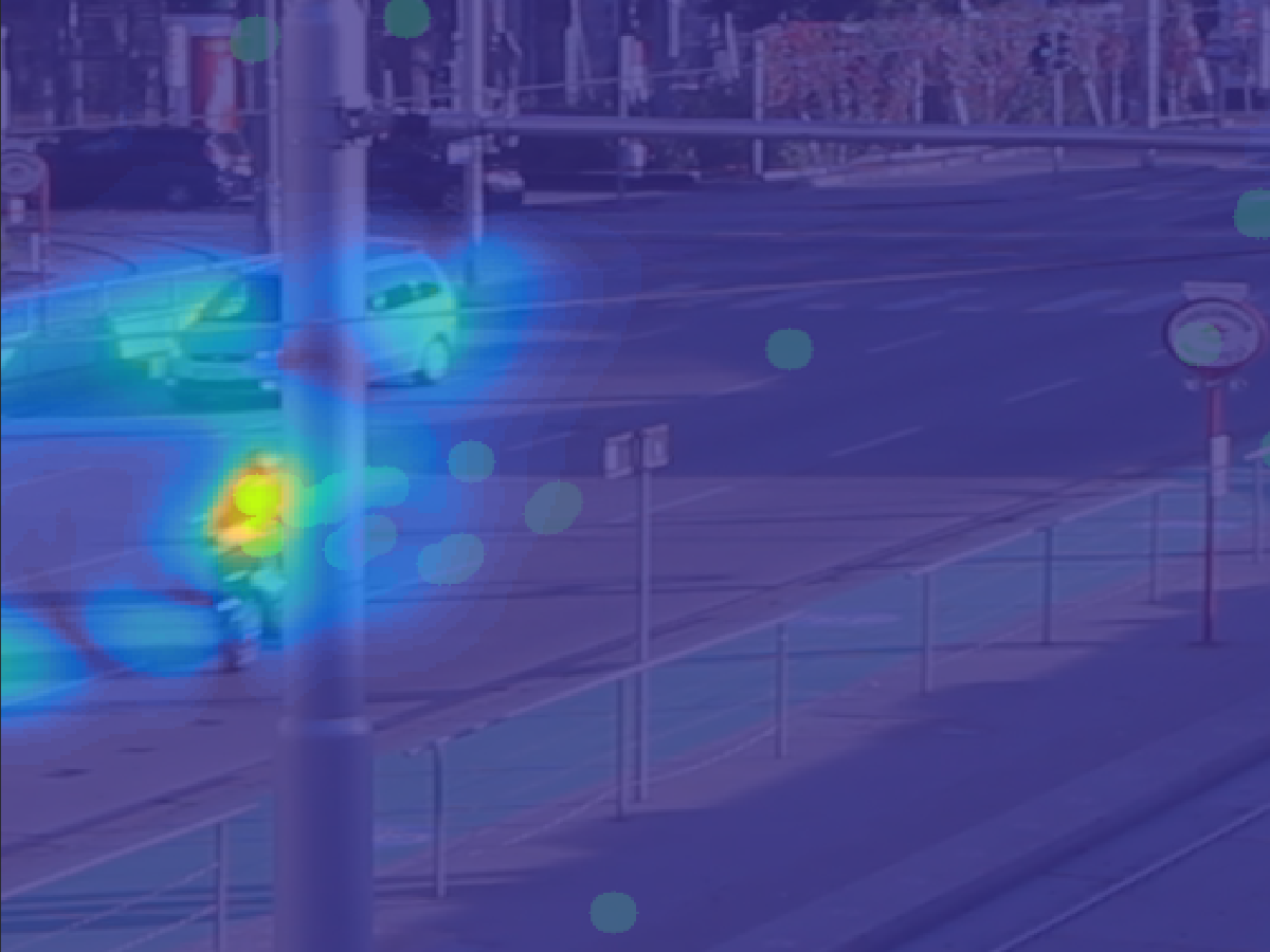
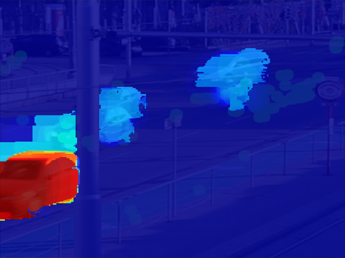
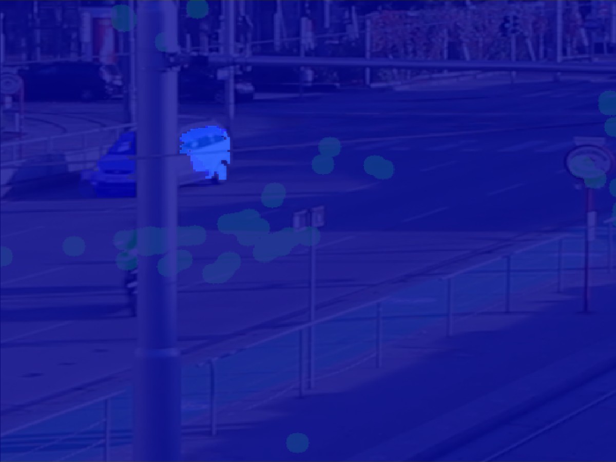
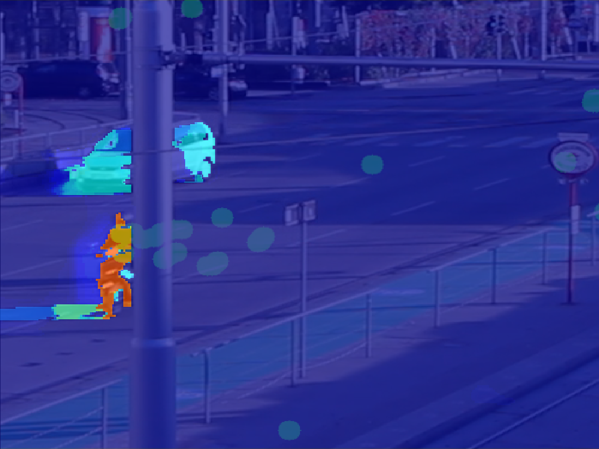
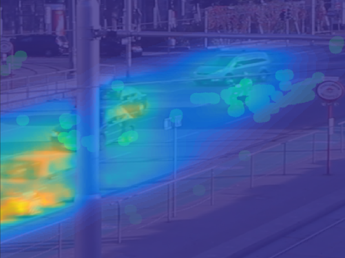
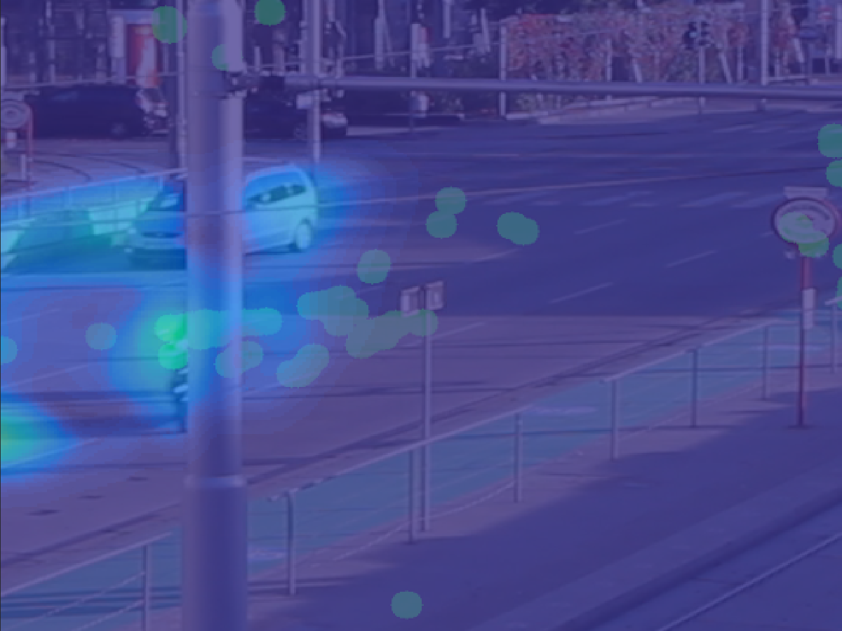
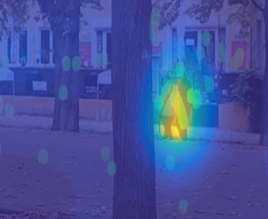
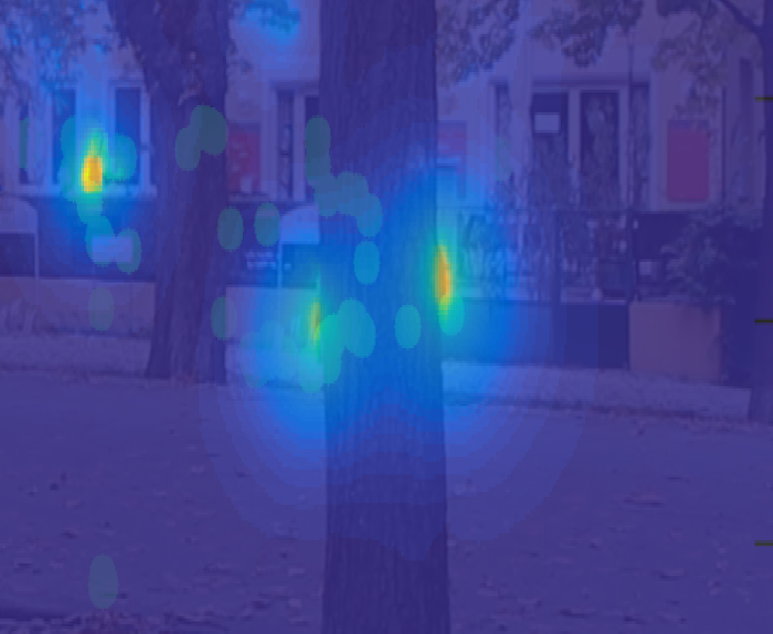
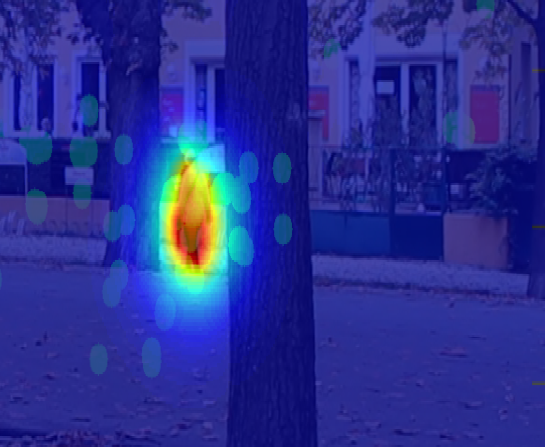
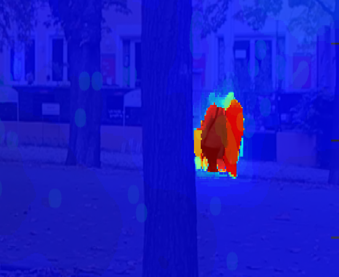
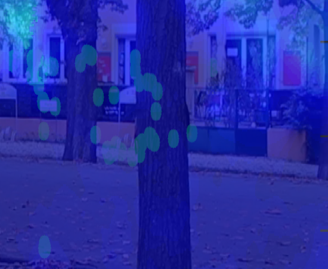
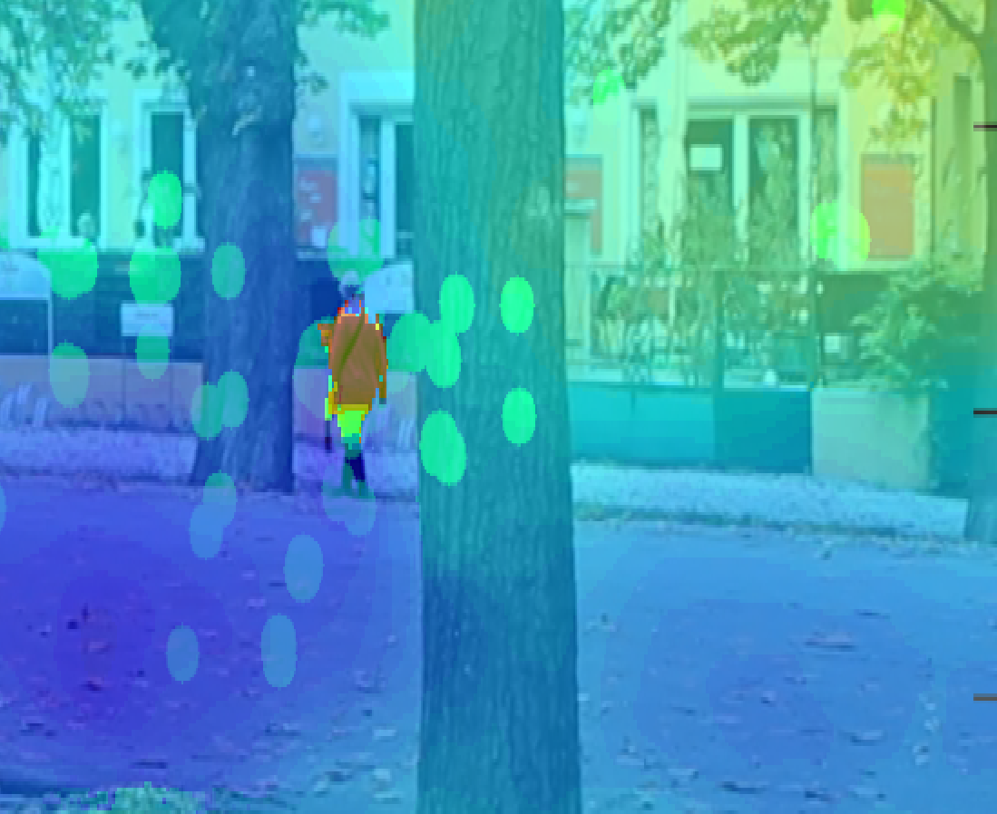
We compare our model (13) with saliency complemented data, with a standard optical flow algorithm [43] and with (13) without complemented data. This last approach is shown to highlight the effect of complementing data with spatial saliency on the calculation of a dynamic saliency map. In order to make a fair comparison between methods, for both our model (13) with gray valued images complemented with saliency and the model of [43] we set the amount of regularization (i.e. $\alpha$) to the value of forty. We set $\alpha=30$ for (13) using color valued images complemented with saliency. Finally, for (13) with both types of complemented data, we set the factor enforcing smoothness over time (i.e $\lambda$) to the value of ten. The parameters for (13) without complemented data are like the one for (13) with complemented data. In Figure 4, 5 and 6 we present three sequences with occlusions. For each sequence we show the results of the models in one frame before, one during, and one after the occlusion. On every depicted frame, we superimposed partecipants’ fixations, with green dots, of the last five frames before until the last five frames after the depicted frame. For the proposed method (13) with complemented data or without complemented data (see Figures 4, 5 and 6 [top and bottom]), the resulting saliency maps are similar for gray valued or color valued images. Therefore, we display only the gray valued version.

Figure 5: The dynamic sequence shows people walking in front of a metro station. A woman in a red coat is walking behind a tree and is salient. We notice that when the woman is occluded (central column), only (13) with saliency complemented data (top) is able to recognize the occluded part as salient. The method considering only two frames [43] (middle) does not recognize this area as salient. The method (13) without complemented data (bottom) results in a lower correlation between the saliency map and the fixation distribution.

Figure 6: The dynamic sequence shows a couple walking in a park. They are walking behind a tree. We notice that when the couple is occluded (central column), only (13) with saliency complemented data (top) is able to recognize the occluded part as salient. The method considering only two frames [43] (middle) does not recognize this area as salient. The method (13) without complemented data (bottom) results in a lower correlation between the saliency map and the fixation distribution. This sequence is particularly challenging due to light reflections and noise. We notice how the method in [43] (middle) is affected by over-smoothing.

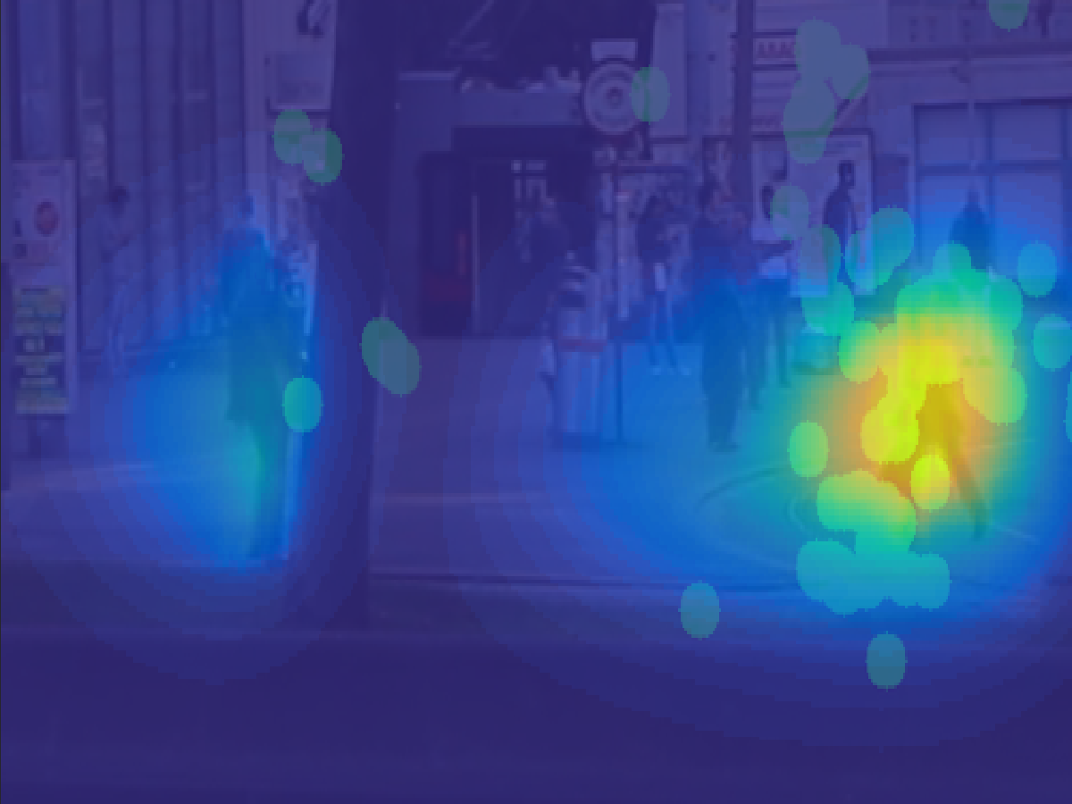
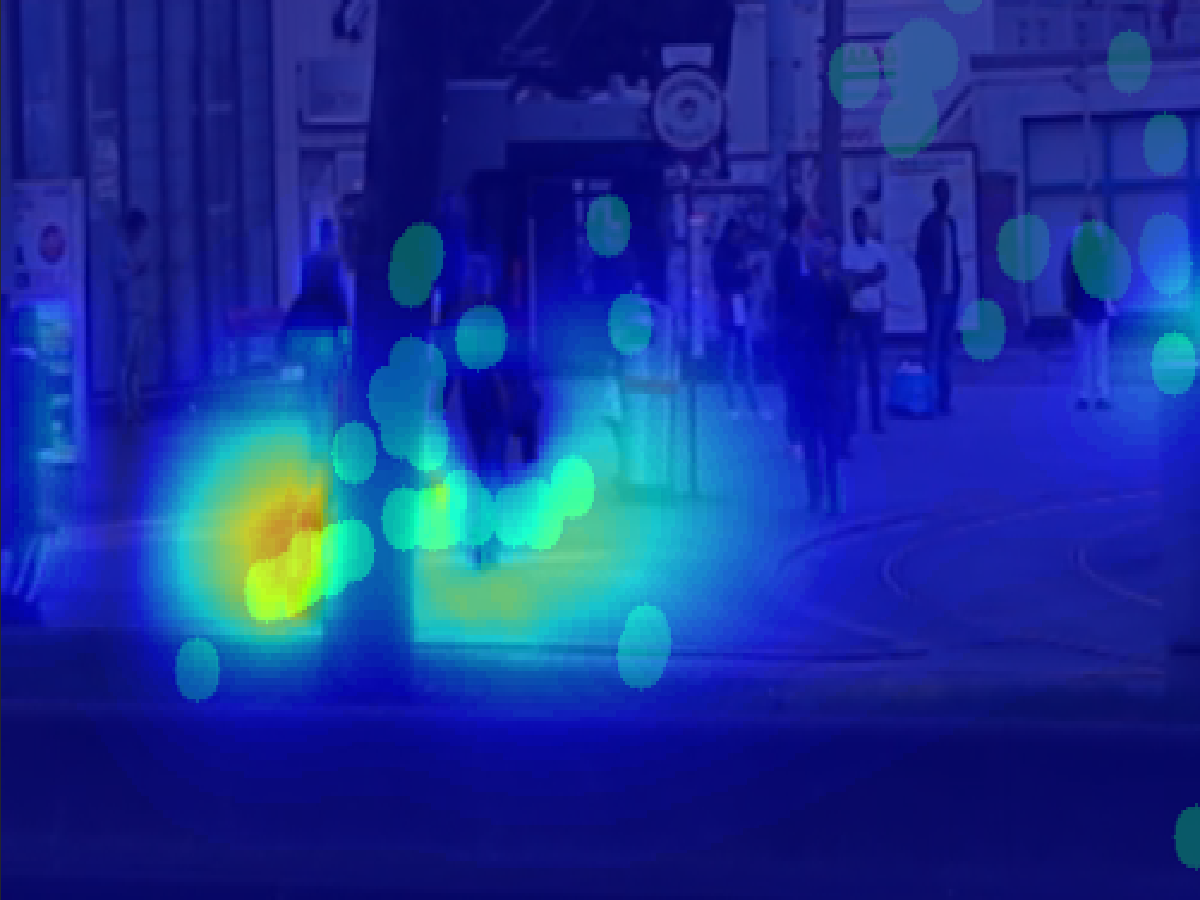
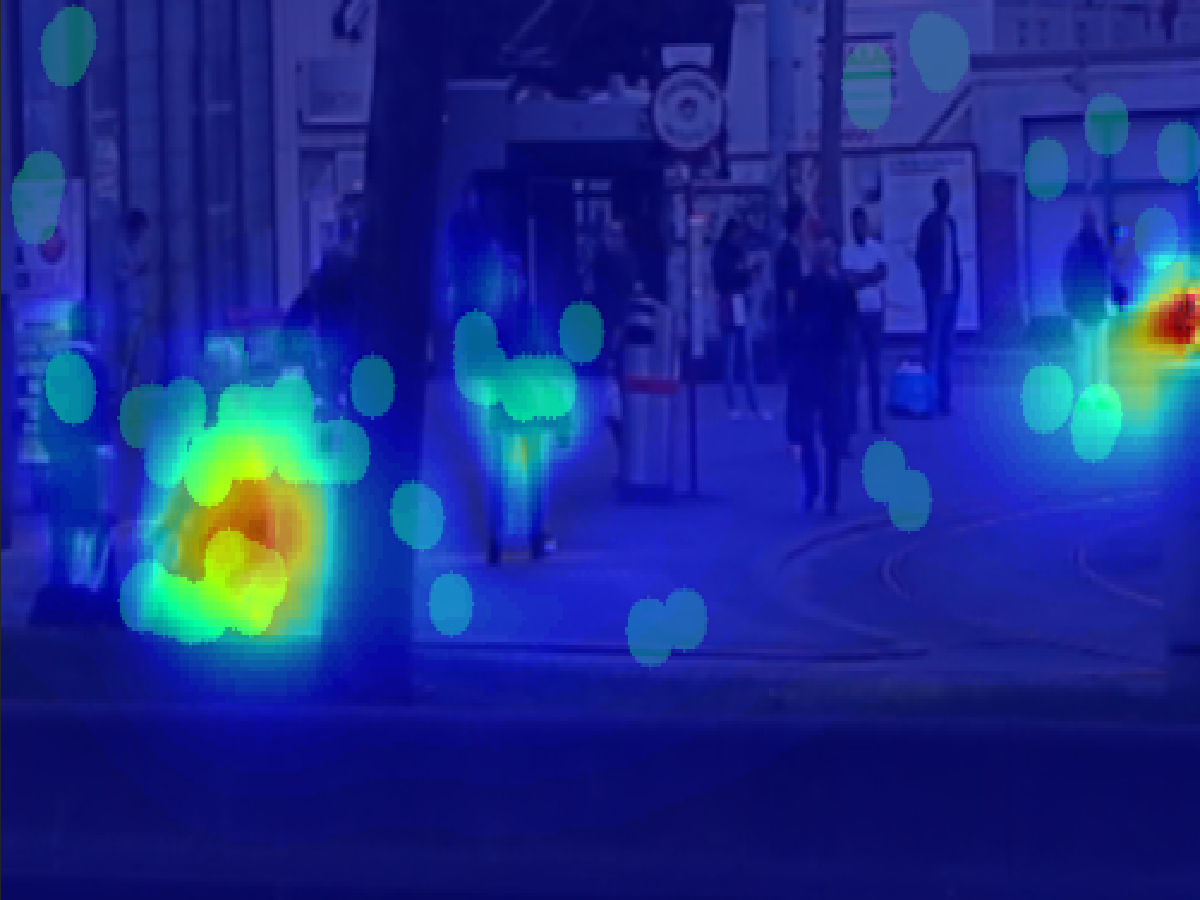
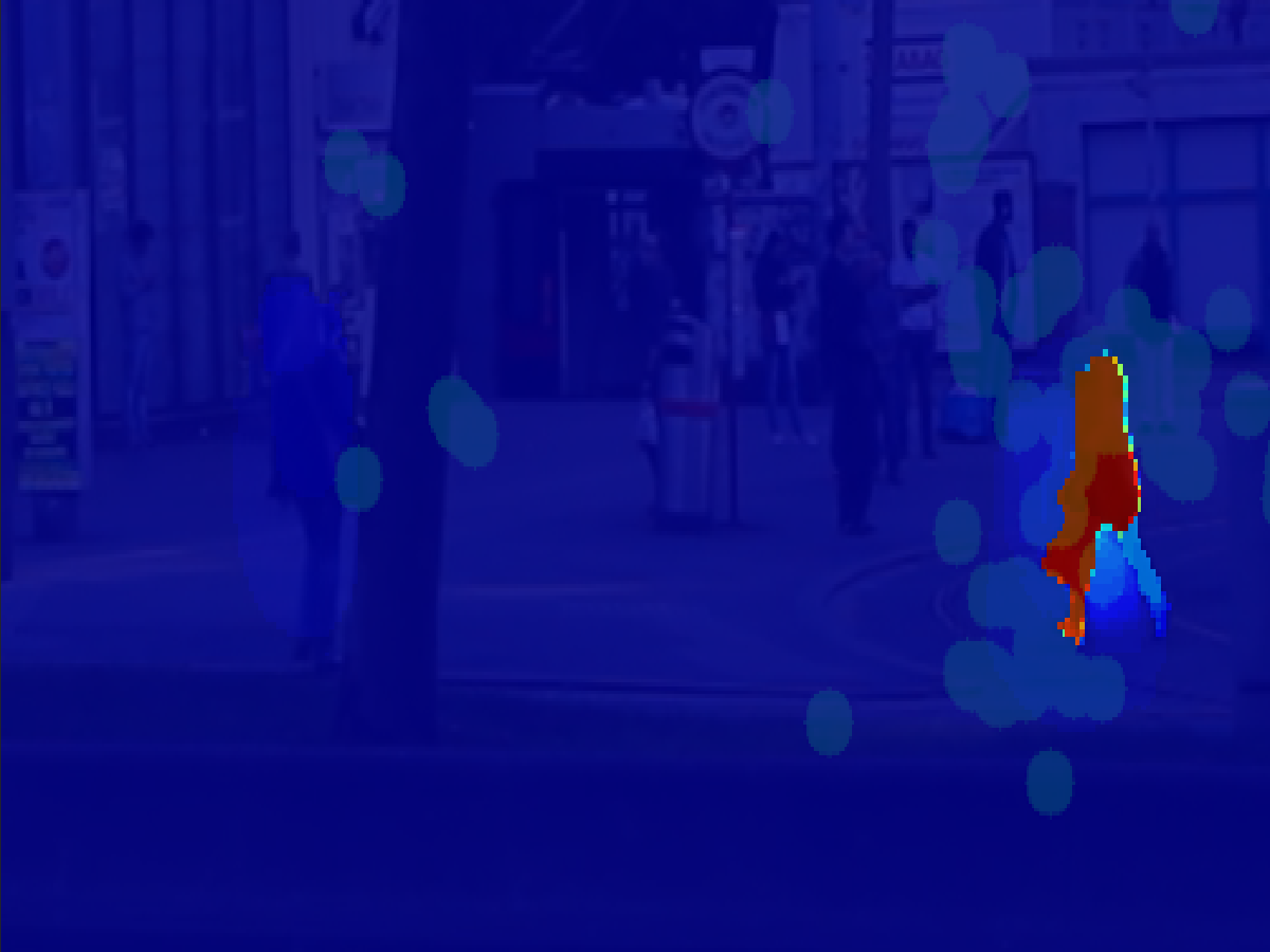
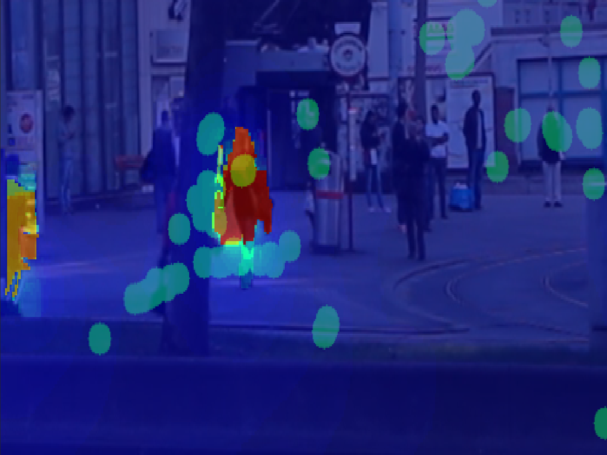
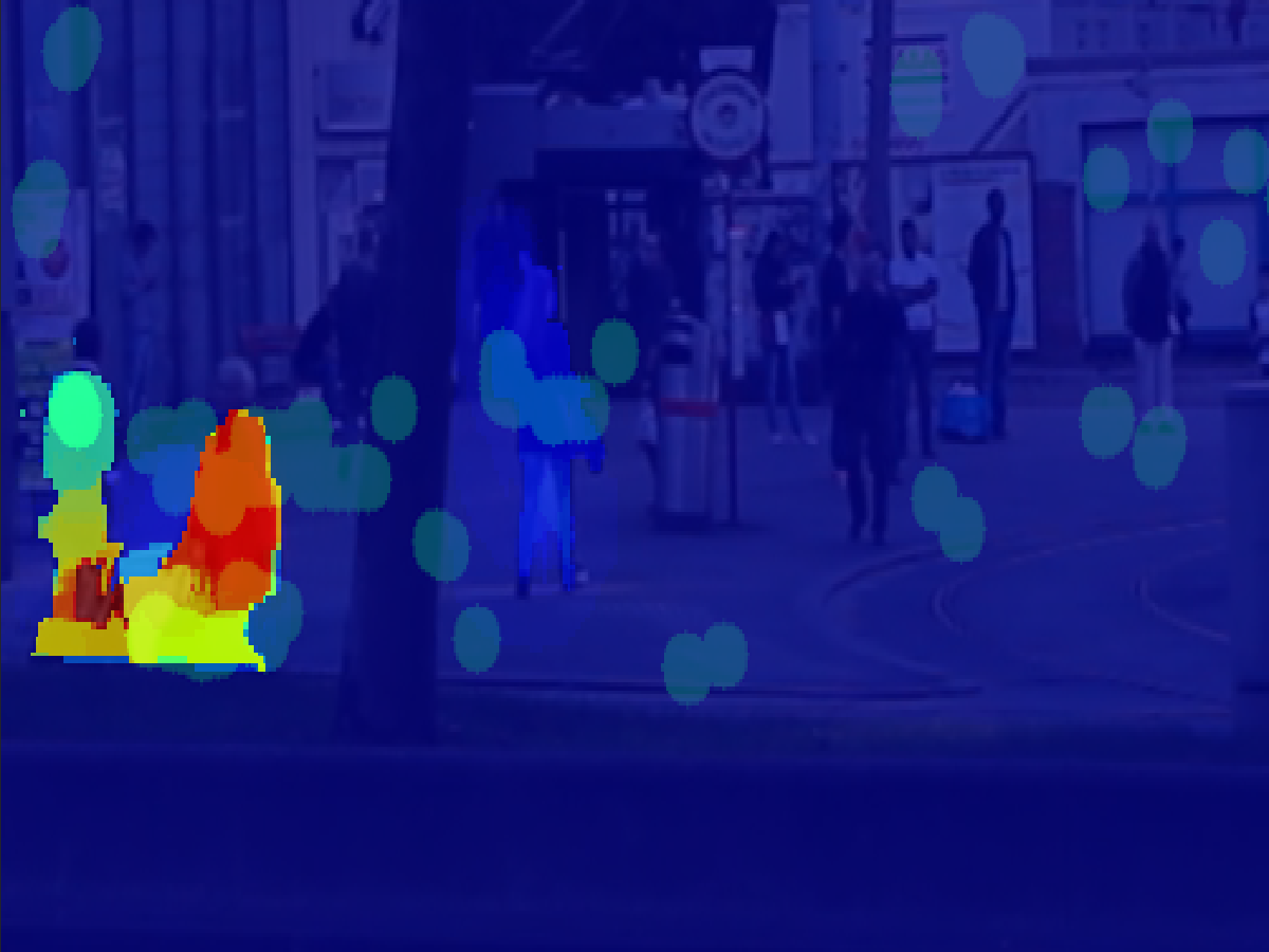
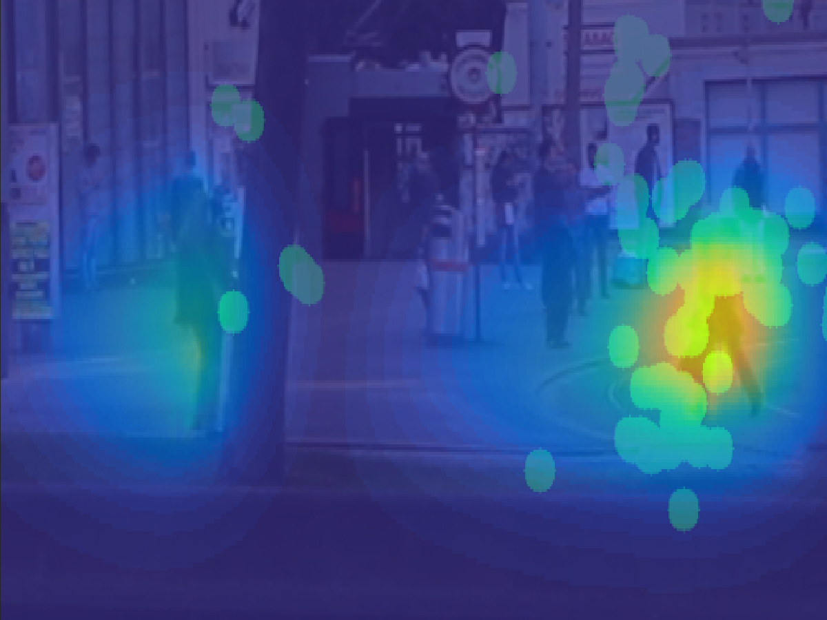
The first video in Figure 4 shows a motorcycle riding behind a pole. We note that people are looking at the pole in order to follow the motion during the occlusion. A two-frame method such as [43] does not recognize the pole as salient, while our method (13) does so for the occluding parts of the pole (see Figure 4 [top]). Moreover, (13) without complemented data recognizes the occlusion as salient, but the area is not as strongly marked as attractive for attention compared to (13) with complemented data. Indeed, we are not able to predict if the people are looking at the car or at the motorcycle in Figure 4. Therefore, the usage of complemented data in (13) results in a better fit to the measured fixations compared to (13) without complemented data (see Figure 5 [top and bottom]) We notice moreover that the method in [43] discards the information regarding the motorcycle in the central column of Figure 4.

In the second video in Figure 5, we see a woman running which is occluded by a tree for some moments. The woman is highly salient due to the strong color contrast of her red coat. Her saliency is not recognized by [43] while the woman is being occluded by a tree. Using both types of complemented data, our method (13) recognizes her saliency correctly. We notice how a two-frame method like [43], in the central column of Figure 5, is affected by over-smoothing, which results in a wrong interpretation. This image illustrates that the temporal coherence inherent in (13) but lacking in [43] makes the method more robust against over-smoothing. Also in this experiment like in the previous one, the usage of complemented data results in a saliency map more correlated to the gaze points compared to the one without complemented data (see Figure 5 [top and bottom]).

Finally, the third video shows a couple walking behind a tree. This sequence is particularly challenging because it includes many points with light reflections and noise. We notice that this does not affect the proposed model (13), but it influences the result of a two-frame model like [43]. This outcome shows that using temporal coherence, as is done in our model (13), results in a robust method, usable for real video sequences. The saliency of the walking couple is correctly recognized by our model (13) using complemented data ( see Figure 6 [top]). Moreover, the model marks the tree section as potentially attractive for attention, a region that the participants indeed fixate during the occlusion (see Figure 6 central column [top]). We notice that in all these experiments the proposed model (13) with complemented data recognizes the salient part of the sequences more clearly compared to (13) without complemented data and to [43].

4.1.1 Model evaluation measures

Figure 7: Comparison according to AUC (top) and NSS (bottom) for the proposed approach (13) with complemented data, the motion as modeled in [6] and a standard optical flow algorithm [43]

As comparison metrics we chose [51]: area under the curve (AUC) of the receiver operating characteristic (ROC) and normalized scanpath saliency (NSS). The AUC treats the saliency map as a classifier. Starting from a saliency map, the AUC algorithm labels all the pixels over a threshold as True Positive (TP) and all the pixels below as False Positive (FP). Human fixations are used as ground truth. This procedure is repeated one hundred times with different threshold values. Finally, the algorithm can estimate the ROC curve and compute the AUC score. A perfect prediction corresponds to a score of 1.0 while a random classification results in 0.5.
The NSS was introduced by [52]. For each point along a subject scan-path we extract the corresponding position $p$ and a partial value is calculated:

$$NSS(p)=\frac{SM(p)-\mu_{SM}}{\sigma_{SM}}$$ (16)

where $SM$ is the saliency map. In (16) we normalize the saliency map in order to have zero mean and unit standard deviation. The final NSS score is the average of $NSS(p)$:

$$NSS=\frac{1}{N}\sum_{p=1}^{N}NSS(p)$$ (17)

where $N$ is the total number of fixation points. The NSS, due to the initial normalization of the saliency map, allows comparison across different subjects. For this measurement the perfect prediction corresponds to a score of 1.0.

In this paper, for the implementation of AUC and NSS we follow [53].
These measures are used to test the prediction performances of our new dynamic saliency map. In other approaches [15, 6, 9, 54, 16, 18] the dynamic saliency maps are combined through a chosen weighting scheme [15, 54] with spatial saliency maps and then the resulting saliency map tested. Here, we do not discuss the choice of a weighting scheme and we test directly the dynamic saliency map.
In Figure 7, we compare the proposed model (13) using the two types of complemented data, the motion as modeled in [6] and a standard optical flow algorithm [43]. We set the regularization parameter $\alpha=40$ for [43]. We notice in Figure 7 that the proposed model (13) performs similarly with both types of complemented data. Moreover, it performs better than the other models considered. It is worth noticing that two frames models such as [43] and [6] have bad performances. This is coherent with our previous results. The algorithms of [43] and [6] discards more information than (13) (as the motorcycle in the central column of Figure 4, second row). Moreover, the models of [43] and of [6] fail in particular cases as the occlusion one described in the previous paragraph.

5 Conclusion

We have proposed a novel dynamic saliency map based on a variational approach and optical flow computations. The framework is applicable to every type of spatial saliency algorithm and results in significant improvements of model performance with regard to predicting human fixations in videos. We analyzed the possibility to use gray valued images or color valued images complemented with spatial saliency as input of our model. Finally, we studied the contribution of temporal coherence for calculating dynamic saliency maps and presented an application regarding occlusions. The results underline better performances (AUC and NSS) explaining visual attention compared to other approaches in literature [6, 43].

6 Acknowledgements

This work is carried out within the project ”Modeling Visual Attention as a Key Factor in Visual Recognition and Quality of Experience” funded by the Wiener Wissenschafts und Technologie Fonds - WWTF (Grant no. CS11-009 to UA and OS). OS is also supported by the Austrian Science Fund - FWF, Project S11704 with the national research network, NFN, Geometry and Simulation. The authors would like to thank P. Elbau for interesting discussions on optical flow. The authors also thank R. Seywerth for help with creating the stimulus videos and collecting the eye tracking data.

Appendix A The use of complemented data results in a more reliable optical flow

We would like to emphasize that the purpose of our model (13) is to estimate the dynamic saliency map of a movie sequence and not calculating a precise optical flow. As shown in Table 1, if we use saliency complemented data in (13), we can calculate the optical flow in imaging regions without regularization. In turn this means that by taking this into account we can reduce the amount of regularization (smaller $\alpha$) in optical flow minimization algorithms.

Figure 8: We test the reliability of the optical flow comparing (13) using gray valued images complemented with spatial saliency (left column), (13) using color valued images complemented with spatial saliency (central column) and (13) using color valued images not complemented (right column). The used comparison measure is the average angular error [36] for the Grove 3 (top) and the Hydrangea (bottom) sequences from the Middleburry dataset. Blue shade color indicates points with small average angular error. For these experiments we set $\tau=0.01$ and $\alpha=0.8$, $\alpha=0.01$ and $\alpha=1.5$, respectively.

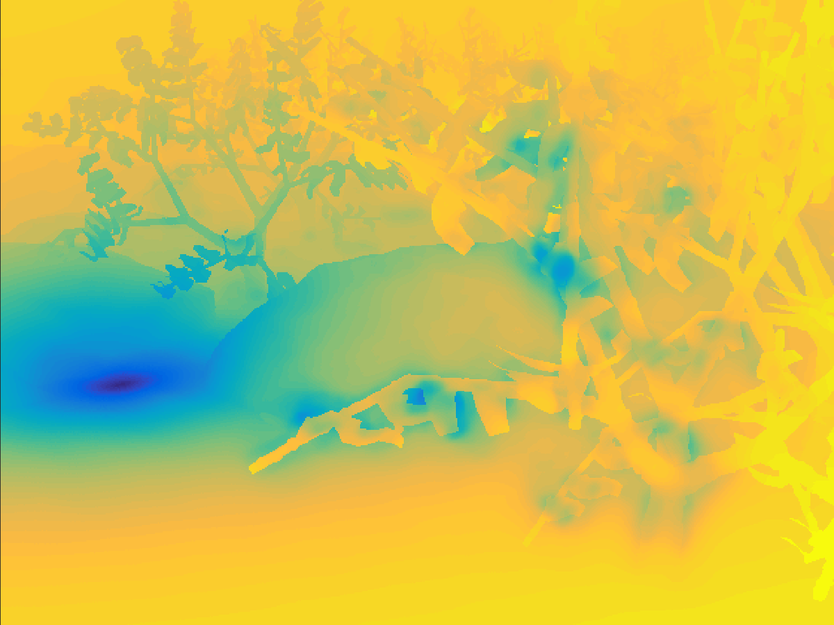
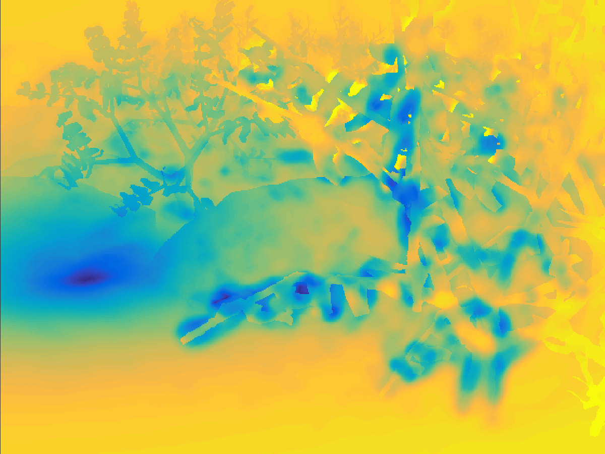
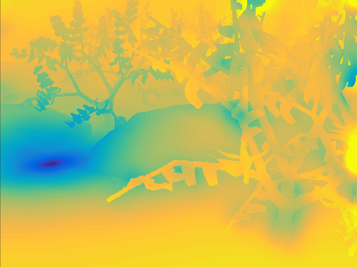
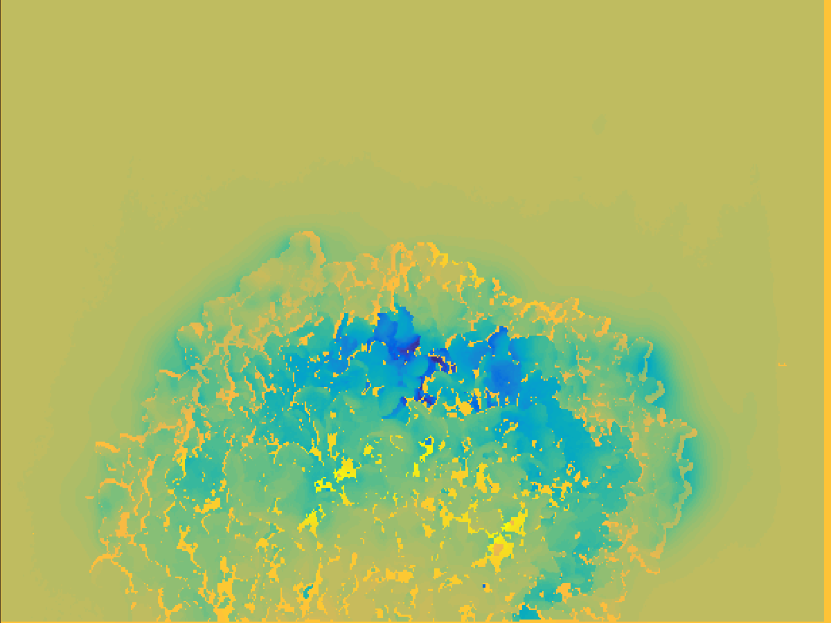
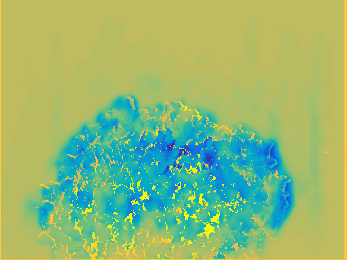
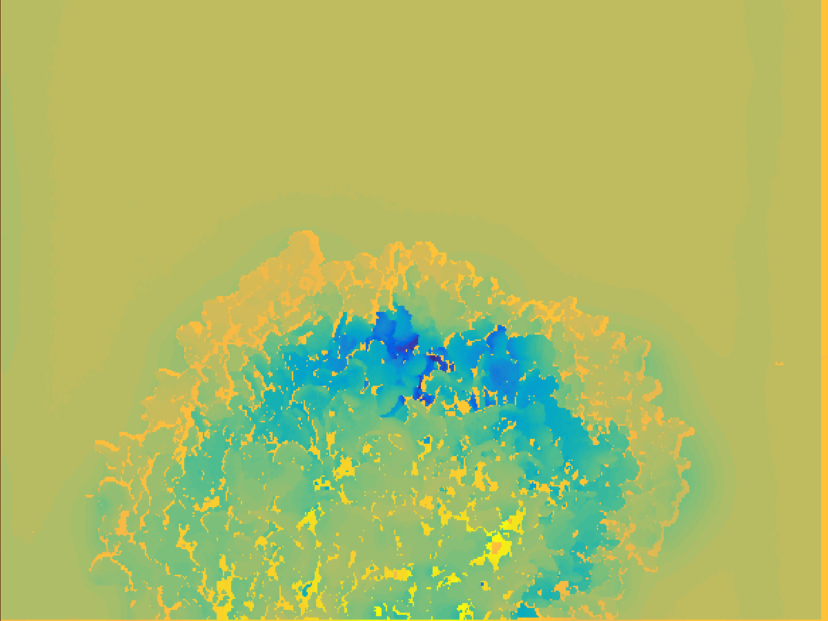
We test the assumptions above for two sequences of the Middlebury dataset [36]. We compare the flow obtained with our complemented data, with the true one, also called ground truth for these sequences. We use the average angular error [42] as comparison measure. In Figure 8, areas colored in shades of blue are the ones for which the average angular error is small. This means that in these areas, the flow is close to the true one.

In accordance with the results in Table 1, we set $\alpha$ to a value of: $0.8$ for gray scale data complemented with saliency, $0.01$ for color valued images complemented by saliency, and $1.5$ for color valued images. Ideally, we should obtain similar areas with small error.

We notice in Figure 8 that the result we obtain by using color valued images complemented with saliency outperforms the other approaches. Moreover, the model (13) that uses gray valued images complemented with saliency performs slightly performs better than the one using only color valued images without saliency. This exemplary test confirms our results in Table 1.

References

- [1] J. M. Henderson, Human gaze control during real-world scene perception, Trends in cognitive sciences 7 (11) (2003) 498–504.
- [2] L. Itti, C. Koch, E. Niebur, A model of saliency-based visual attention for rapid scene analysis, IEEE Transactions on Pattern Analysis & Machine Intelligence 20 (11) (1998) 1254–1259.
- [3] J. Harel, C. Koch, P. Perona, Graph-based visual saliency, in: Advances in neural information processing systems, 2006, pp. 545–552.
- [4] U. Rajashekar, I. Van Der Linde, A. C. Bovik, L. K. Cormack, Gaffe: A gaze-attentive fixation finding engine, Image Processing, IEEE Transactions on 17 (4) (2008) 564–573.
- [5] R. Achanta, S. Hemami, F. Estrada, S. Susstrunk, Frequency-tuned salient region detection, in: Computer vision and pattern recognition, 2009. cvpr 2009. ieee conference on, IEEE, 2009, pp. 1597–1604.
- [6] C. Guo, L. Zhang, A novel multiresolution spatiotemporal saliency detection model and its applications in image and video compression, Image Processing, IEEE Transactions on 19 (1) (2010) 185–198.
- [7] Y. Fang, Z. Wang, W. Lin, Z. Fang, Video saliency incorporating spatiotemporal cues and uncertainty weighting, Image Processing, IEEE Transactions on 23 (9) (2014) 3910–3921.
- [8] L. Itti, P. F. Baldi, Bayesian surprise attracts human attention, in: Advances in neural information processing systems, 2005, pp. 547–554.
- [9] L. Itti, P. Baldi, A principled approach to detecting surprising events in video, in: Computer Vision and Pattern Recognition, 2005. CVPR 2005. IEEE Computer Society Conference on, Vol. 1, IEEE, 2005, pp. 631–637.
- [10] L. Itti, C. Koch, Computational modelling of visual attention, Nature reviews neuroscience 2 (3) (2001) 194–203.
- [11] C. Liu, P. C. Yuen, G. Qiu, Object motion detection using information theoretic spatio-temporal saliency, Pattern Recognition 42 (11) (2009) 2897–2906.
- [12] Z. Ren, S. Gao, L.-T. Chia, D. Rajan, Regularized feature reconstruction for spatio-temporal saliency detection, Image Processing, IEEE Transactions on 22 (8) (2013) 3120–3132.
- [13] S. Li, M. C. Lee, Fast visual tracking using motion saliency in video, in: Acoustics, Speech and Signal Processing, 2007. ICASSP 2007. IEEE International Conference on, Vol. 1, IEEE, 2007, pp. I–1073.
- [14] Y.-F. Ma, H.-J. Zhang, A model of motion attention for video skimming, in: Image Processing. 2002. Proceedings. 2002 International Conference on, Vol. 1, IEEE, 2002, pp. I–129.
- [15] S. Marat, T. Ho Phuoc, L. Granjon, N. Guyader, D. Pellerin, A. Guérin-Dugué, Spatio-temporal saliency model to predict eye movements in video free viewing, in: Signal Processing Conference, 2008 16th European, IEEE, 2008, pp. 1–5.
- [16] R. J. Peters, L. Itti, Beyond bottom-up: Incorporating task-dependent influences into a computational model of spatial attention, in: Computer Vision and Pattern Recognition, 2007. CVPR’07. IEEE Conference on, IEEE, 2007, pp. 1–8.
- [17] A. C. Schütz, D. I. Braun, K. R. Gegenfurtner, Object recognition during foveating eye movements, Vision research 49 (18) (2009) 2241–2253.
- [18] L. Zhang, M. H. Tong, G. W. Cottrell, Sunday: Saliency using natural statistics for dynamic analysis of scenes, in: Proceedings of the 31st Annual Cognitive Science Conference, AAAI Press Cambridge, MA, 2009, pp. 2944–2949.
- [19] D. Gao, N. Vasconcelos, Discriminant saliency for visual recognition from cluttered scenes, in: Advances in neural information processing systems, 2004, pp. 481–488.
- [20] J. K. Tsotsos, S. M. Culhane, W. Y. K. Wai, Y. Lai, N. Davis, F. Nuflo, Modeling visual attention via selective tuning, Artificial intelligence 78 (1) (1995) 507–545.
- [21] S. Vijayakumar, J. Conradt, T. Shibata, S. Schaal, Overt visual attention for a humanoid robot, in: Intelligent Robots and Systems, 2001. Proceedings. 2001 IEEE/RSJ International Conference on, Vol. 4, IEEE, 2001, pp. 2332–2337.
- [22] B. K. Horn, B. G. Schunck, Determining optical flow, in: 1981 Technical symposium east, International Society for Optics and Photonics, 1981, pp. 319–331.
- [23] O. Scherzer, M. Grasmair, H. Grossauer, M. Haltmeier, F. Lenzen, Variational methods in imaging, Vol. 2, Springer, 2009.
- [24] J. Weickert, C. Schnörr, Variational optic flow computation with a spatio-temporal smoothness constraint, Journal of Mathematical Imaging and Vision 14 (3) (2001) 245–255.
- [25] P. Anandan, A computational framework and an algorithm for the measurement of visual motion, International Journal of Computer Vision 2 (3) (1989) 283–310.
- [26] M. J. Black, P. Anandan, The robust estimation of multiple motions: Parametric and piecewise-smooth flow fields, Computer vision and image understanding 63 (1) (1996) 75–104.
- [27] A. Bruhn, J. Weickert, C. Schnörr, Lucas/Kanade meets Horn/Schunck: Combining local and global optic flow methods, International Journal of Computer Vision 61 (3) (2005) 211–231.
- [28] E. Mémin, P. Pérez, Dense estimation and object-based segmentation of the optical flow with robust techniques, Image Processing, IEEE Transactions on 7 (5) (1998) 703–719.
- [29] E. Mémin, P. Pérez, A multigrid approach for hierarchical motion estimation, in: Computer Vision, 1998. Sixth International Conference on, IEEE, 1998, pp. 933–938.
- [30] E. Mémin, P. Pérez, Hierarchical estimation and segmentation of dense motion fields, International Journal of Computer Vision 46 (2) (2002) 129–155.
- [31] R. Andreev, O. Scherzer, W. Zulehner, \hrefhttp://dx.doi.org/10.1016/j.apnum.2015.04.007Simultaneous optical flow and source estimation: Space–time discretization and preconditioning, Applied Numerical Mathematics 96 (2015) 72–81. \hrefhttp://dx.doi.org/10.1016/j.apnum.2015.04.007 doi:10.1016/j.apnum.2015.04.007.
- [32] A. Borzi, K. Ito, K. Kunisch, Optimal control formulation for determining optical flow, SIAM journal on scientific computing 24 (3) (2003) 818–847.
- [33] A. R. Patrone, O. Scherzer, On a spatial-temporal decomposition of the optical flow, arXiv preprint arXiv:1505.03505.
- [34] C.-M. Wang, K.-C. Fan, C.-T. Wang, Estimating optical flow by integrating multi-frame information., J. Inf. Sci. Eng. 24 (6) (2008) 1719–1731.
- [35] J. Weickert, C. Schnörr, A theoretical framework for convex regularizers in pde-based computation of image motion, International Journal of Computer Vision 45 (3) (2001) 245–264.
- [36] S. Baker, D. Scharstein, J. Lewis, S. Roth, M. J. Black, R. Szeliski, A database and evaluation methodology for optical flow, International Journal of Computer Vision 92 (1) (2011) 1–31.
- [37] J. A. Iglesias, C. Kirisits, Convective regularization for optical flow, arXiv preprint arXiv:1505.04938.
- [38] S.-H. Lai, B. C. Vemuri, Reliable and efficient computation of optical flow, International Journal of Computer Vision 29 (2) (1998) 87–105.
- [39] H. Zimmer, A. Bruhn, J. Weickert, Optic flow in harmony, International Journal of Computer Vision 93 (3) (2011) 368–388.
- [40] T. Brox, A. Bruhn, N. Papenberg, J. Weickert, High accuracy optical flow estimation based on a theory for warping, in: Computer Vision-ECCV 2004, Springer, 2004, pp. 25–36.
- [41] M. Lefébure, L. D. Cohen, Image registration, optical flow and local rigidity, Journal of Mathematical Imaging and Vision 14 (2) (2001) 131–147.
- [42] J. L. Barron, D. J. Fleet, S. S. Beauchemin, Performance of optical flow techniques, International journal of computer vision 12 (1) (1994) 43–77.
- [43] D. Sun, S. Roth, M. J. Black, A quantitative analysis of current practices in optical flow estimation and the principles behind them, International Journal of Computer Vision 106 (2) (2014) 115–137.
- [44] M. Dorr, T. Martinetz, K. R. Gegenfurtner, E. Barth, Variability of eye movements when viewing dynamic natural scenes, Journal of vision 10 (10) (2010) 28.
- [45] D. H. Brainard, The psychophysics toolbox, Spatial vision 10 (1997) 433–436.
- [46] F. W. Cornelissen, E. M. Peters, J. Palmer, The eyelink toolbox: eye tracking with matlab and the psychophysics toolbox, Behavior Research Methods, Instruments, & Computers 34 (4) (2002) 613–617.
- [47] D. G. Pelli, The videotoolbox software for visual psychophysics: Transforming numbers into movies, Spatial vision 10 (4) (1997) 437–442.
- [48] G. A. Alvarez, T. S. Horowitz, H. C. Arsenio, J. S. DiMase, J. M. Wolfe, Do multielement visual tracking and visual search draw continuously on the same visual attention resources?, Journal of Experimental Psychology: Human Perception and Performance 31 (4) (2005) 643.
- [49] J. I. Flombaum, B. J. Scholl, Z. W. Pylyshyn, Attentional resources in visual tracking through occlusion: The high-beams effect, Cognition 107 (3) (2008) 904–931.
- [50] B. J. Scholl, Z. W. Pylyshyn, Tracking multiple items through occlusion: Clues to visual objecthood, Cognitive psychology 38 (2) (1999) 259–290.
- [51] N. Riche, M. Duvinage, M. Mancas, B. Gosselin, T. Dutoit, Saliency and human fixations: state-of-the-art and study of comparison metrics, in: Computer Vision (ICCV), 2013 IEEE International Conference on, IEEE, 2013, pp. 1153–1160.
- [52] R. J. Peters, A. Iyer, L. Itti, C. Koch, Components of bottom-up gaze allocation in natural images, Vision research 45 (18) (2005) 2397–2416.
- [53] T. Judd, F. Durand, A. Torralba, \hrefhttp://hdl.handle.net/1721.1/68590A benchmark of computational models of saliency to predict human fixations, Tech. rep., MIT tech report (2012).
- [54] N. Ouerhani, Visual attention: from bio-inspired modeling to real-time implementation, Ph.D. thesis, Université de Neuchâtel (12 2004).