An adaptive moving mesh finite element solution of the Regularized Long Wave equation
Abstract
An adaptive moving mesh finite element method is proposed for the numerical solution of the regularized long wave (RLW) equation. A moving mesh strategy based on the so-called moving mesh PDE is used to adaptively move the mesh to improve computational accuracy and efficiency. The RLW equation represents a class of partial differential equations containing spatial-time mixed derivatives. For the numerical solution of those equations, a finite element method cannot apply directly on a moving mesh since the mixed derivatives of the finite element approximation may not be defined. To avoid this difficulty, a new variable is introduced and the RLW equation is rewritten into a system of two coupled equations. The system is then discretized using linear finite elements in space and the fifth-order Radau IIA scheme in time. A range of numerical examples in one and two dimensions, including the RLW equation with one or two solitary waves and special initial conditions that lead to the undular bore and solitary train solutions, are presented. Numerical results demonstrate that the method has a second order convergence and is able to move and adapt the mesh to the evolving features in the solution.
AMS 2010 Mathematics Subject Classification. 65M50,65M60, 35G61
Key Words. regularized long wave equation, RLW equation, moving mesh, adaptation, finite element method
Abbreviated title. An adaptive moving mesh FE solution of RLW
1 Introduction
We consider the adaptive moving mesh finite element (FE) solution of the regularized long wave (RLW) equation (which is also called the Benjamin-Bona-Mahony or BBM equation) in one and two dimensions. The initial-boundary value problem of the 2D RLW equation [2, 10, 18] reads as
| (1) |
where is a bounded polygonal domain and , , , , are constants with , and , and and are given functions. The RLW equation has been used to model ion acoustic waves and magnetohydrodynamics waves in plasmas, longitudinal dispersive waves in elastic rods, pressure waves in liquid gas bubbles, and nonlinear transverse waves in shallow water; for example see [5, 6, 41]. The RLW equation was proposed first by Peregrine [41] and later by Benjamin et al. [5] as a model for small amplitude long waves on the surface of water in a channel. Generalizations such as the generalized regularized long wave equation (gRLW) or the modified regularized long wave equation (MRLW) [2, 10, 18] and generalized Rosenau-Kawhara-RLW equation [42] also arise from various applications.
The RLW equation is related to the Korteweg-de Vries (KdV) equation but has distinct features. For example, Medeiros and Miranda [36] discuss the problem of periodic solution and show that RLW can almost cover all the application of KdV. On the other hand, Olver [40] proves that RLW can have only three non-trivial independent conservation laws. This is very different from KdV which is known to have an infinite number of conservation laws. Moreover, KdV is known to possess single and multiple solitons that maintain their shapes and velocities after their interactions and can have inelastic collision. RLW does not appear to admit an inverse-scattering theory which would lead to an analytical representation for solitary wave solutions. Nevertheless, the initial-value problem of RLW posed on the whole real line still has the property that initial disturbances resolve into a train of solitary waves and a dispersive tail (e.g., see [7]; also see Examples 4.4 and 4.7 in section 4). Much effort has been made to understand whether or not RLW has the characteristics of solitons. For example, Abdulloev [1] shows that two solitons of RLW can have inelastic collision. Analytical solutions have also been obtained by various researchers; e.g., see [34, 35, 47, 48].
The numerical solution of the RLW equation and its variants and generalizations have been considered extensively in recent decades. Among many existing works, we mention Eilbeck and McGuire [14, 15] (finite difference methods), Guo and Cao [21] (a Fourier pseudospectral method with a restrain operator), Luo and Liu [33] (a mixed Galerkin), Zaki [49] (combined splitting with cubic B-spline FEM), Dogan [13] (linear FEM), Daǧ et al. [11] (cubic B-spline collation), Gu and Chen [20] (a least squares mixed Galerkin), Gao et al. [16] (local Discontinuous Galerkin), Mei et al. [17, 37, 38, 39] (mixed Galerkin), and Siraj-ul-Islam et al. [44] (meshfree method). These works are for RLW, gRLW, or MRLW in 1D, and much less work has been done in 2D. Dehghan and Salehi [12] consider the numerical solution of 2D RLW in fluids and plasmas using the boundary knot method (a meshless boundary-type radial basis function collocation technique).
The objective of this paper is twofold. The first is to study the numerical solution of RLW using an adaptive moving mesh method. The method works for a general spatial dimension but we focus only on 1D and 2D in this work. As will be seen in section 4, a large spatial domain often has to be used in the numerical solution to reduce the boundary effects and to cover the evolving features for the whole time period under consideration. This requires a large number of mesh elements for a reasonable level of computational accuracy especially in multi-dimensions. To improve computational efficiency, it is natural to employ an adaptive moving mesh technique which dynamically adapts the mesh to the local, evolving features in the solution of RLW. In this work, we will employ the so-called moving mesh PDE (MMPDE) method [27, 28, 29] that moves the mesh continuously in time and orderly in space using a PDE formulated as the gradient flow equation of a meshing functional. We will use a newly developed discretization of the MMPDE [25] that makes the implementation of the MMPDE method not only significantly simpler in multi-dimensions but also much more reliable in the sense that there is a theoretical guarantee for mesh nonsingularity.
The second objective of the paper is to study how to discretize space-time mixed derivatives using finite elements on moving meshes. RLW (1) represents a class of PDEs containing space-time mixed derivatives. In addition to RLW, this class includes Boussinesq [9], modified Buckley-Leverett [45], and Sobolev [43] equations. A feature of these PDEs is that space-time mixed derivatives are involved in their both strong and weak formulations. When the mesh is moving, these derivatives of a finite element approximation are not defined (cf. section 2.1). There are various ways to overcome this difficulty. We utilize a new variable (see (2) below) and demonstrate numerically that the resulting linear finite element discretization gives a second order convergence on moving meshes. Since (2) is not tailored to the special structure of RLW, we may expect that this idea of treating space-time mixed derivatives can also be used for the moving mesh solution of Boussinesq, modified Buckley-Leverett, and Sobolev equations.
It is worth mentioning that a number of moving mesh methods have been developed in the past and there is a considerable literature in the area. Instead of going over the literature, we refer the interested reader to the books/review articles [3, 4, 8, 29, 46] and references therein.
An outline of the paper is as follows. The adaptive moving mesh finite element method is described in Section 2. The transformation of RLW into a system of two coupled PDEs, the discretization of the PDE system on moving meshes via linear finite elements, and the conservation laws possessed by RLW are discussed in the section. The generation of adaptive moving meshes using a new implementation of the MMPDE method is discussed in section 3. 1D and 2D numerical examples of RLW (and MRLW) are presented in section 4. Finally, section 5 contains conclusions and further comments.
2 An adaptive moving mesh finite element method
In this section we describe the adaptive moving mesh FE method for the numerical solution of the RLW equation. We first describe the basic procedure of the method and then elaborate on the linear FE discretization of the RLW equation on moving meshes, followed by a discussion on the conservation laws possessed by the RLW equation. An MMPDE-based moving mesh strategy will be discussed in the next section. To be specific, we describe the method in two dimensions. The one dimensional formulation is similar.
We start with introducing a new variable
| (2) |
and rewriting (1) into
| (3) |
The weak formulation is to find and for such that
| (4) |
The basic procedure of the the adaptive moving mesh FE method for solving (4) is as follows.
-
1.
Given an initial mesh and an initial time step .
-
2.
For
-
(a)
An MMPDE-based moving mesh strategy (cf. section 3) is used to generate the new mesh based on the current mesh and the numerical solution defined thereon. Note that and have the same number of the elements (), the same number of the vertices (), and the same connectivity. They differ only in the location of the vertices, , .
-
(b)
For with , the coordinates and velocities of the vertices are defined as
The corresponding mesh is denoted by ().
-
(c)
The RLW equation (4) is discretized in space using linear finite elements and then integrated in time for one step using the fifth-order Radau IIA method (e.g., see Hairer and Wanner [22]). A standard procedure is used for the selection of the time step size, together with a two-step error estimator of González-Pinto et al. [19]. If the actual step size (denoted by ) is smaller than , the time and mesh are updated as
The predicted time step size will be used as .
-
(a)
The FEM discretization of the RLW equation on is discussed in the next subsection while the generation of using the MMPDE-based moving mesh strategy will be given in section 3.
2.1 Linear finite element discretization on
For notational simplicity, we assume that the vertices of are ordered in a way that the first vertices are interior vertices. Let be the linear basis function associated with the -th vertex . Define
| (5) | |||
| (6) | |||
| (7) |
The linear finite element approximation of (4) is to find and , such that
| (8) |
To cast (8) in a matrix form, we express and as
| (9) |
subject to the boundary condition
| (10) |
Notice that
It is not difficult to show (e.g., see Jimack and Wathen [31]) that
| (11) |
where is a piecewise linear mesh velocity defined by
| (12) |
Using this we can rewrite as
| (13) |
Inserting (9), (10), and (13) into (8) and taking () and () successively, we get
| (14) |
where the vectors and matrices in (14) are partitioned according to the entries associated with the interior vertices (with symbol “”) and those associated with the boundary vertices (with symbol “”), and are the unknown vectors, and are the mass and stiffness matrices, respectively, and the entries of , , , and are given by
| (15) |
When the mesh is fixed, both the mass and stiffness matrices are time independent. In this case, by differentiating the second equation of (14) with respect to time and subtracting it from the first equation we get
| (16) |
Since both and are symmetric and positive definite, is invertible and (16) forms an ODE system. As a result, the solution existence and uniqueness of (14) can be derived from that of the ODE system (16). Moreover, it is not difficult to show that (16) can also be obtained by applying the linear finite element discretization directly to the original equation (1).
When the mesh is varying with time, both and depend on time too. In this case, (14) cannot reduce to (16) in general. Nevertheless, from the second and third equations of (14) we get
| (17) |
Notice that is a function of and can be written as . Inserting (17) into the first equation of (14) we obtain
| (18) |
which is also an ODE system. Then, the solution existence and uniqueness of (14) can be derived from that of the ODE system (18). Once has been obtained, we can find from (17).
In our computation, (14) is solved directly, which is a DAE (differential-algebraic equation) system. It is integrated using the fifth-order Radau IIA method with a variable step size determined by a two-step error estimator of Gonzalez-Pinto et al. [19].
Remark 2.1.
On a moving mesh, a finite element method cannot be applied to the original equation (1) directly. Indeed, the weak formulation of (1) takes the form
Then a finite element approximation will contain space-time mixed derivatives
| (19) |
where is a finite element approximation to . Notice that is piecewise continuous and is discontinuous across element boundaries. Since these boundaries vary with time for a moving mesh, has jumps in the time direction for spatial points where the element boundaries sweep through (see Fig. 1) and cannot be differentiated with respect to time at these points (even in weak sense). Thus, the terms in (19) are not defined on , and a moving mesh finite element method does not apply to (1) directly. ∎
Remark 2.2.
Several other choices of new variables have been used in the numerical solution of the RLW equation. For example, Luo and Liu [33] (also see Gu and Chen [20] for a least squares mixed FEM) use the new variable for a mixed finite element approximation of the 1D RLW equation
subject to a homogeneous Dirichlet boundary condition. They use the weak formulation
It does not work with a moving mesh finite element method since it contains space-time mixed derivatives. More recently, Gao and Mei [17] define for the 1D RLW equation
with a homogeneous Dirichlet boundary condition. They use the weak formulation
which once again does not work with a moving mesh finite element method since it contains a space-time mixed derivative. ∎
2.2 Conservation laws
Olver [40] shows that the RLW equation possesses three non-trivial independent conservation laws. Each of such laws corresponds to an invariant quantity if the solution vanishes on the boundary (i.e., ). The first two for (1) are
| (20) |
which can readily be verified by multiplying (1) with and , respectively, integrating the resulting equation over , and performing integration by parts.
We first consider if these quantities are conserved by the finite element approximation on a fixed mesh. For this case, and both and are independent of time. Summing the rows of (16) and using (15) and , we have
This can be rewritten as
Noticing that and using the divergence theorem and the fact that , we obtain
| (21) |
Thus, is not conserved by (16) since the right-hand side does not vanish in general. An estimate of the derivation can be obtained as follows. Noticing that and using Schwarz’s inequality, we have
Assuming that the finite element error is second order in norm, we have
| (22) |
where is the maximal diameter of the elements. It is interesting to point out that the numerical examples in section 4 show that the difference decreases much faster than what shown in (22) as . This may be attributed to the cancellation between terms on the right-hand side of (21) and the fact that and its derivatives are getting smaller on the boundary elements which are getting closer to the boundary as increases.
Similarly, multiplying the -th row of (16) with and summing all of the resulting rows we can get
| (23) |
which implies that is conserved by (16). It is noted that this conservation holds only for the semi-discrete scheme (16). It may not necessarily hold for the fully discrete scheme. Nevertheless, (23) implies that the difference will be small when the time step is small.
We now consider the moving mesh situation. Generally speaking, and both and are time dependent for this case. In principle, we can perform a similar analysis as for the fixed mesh case. Since the derivation is very tedious and the results are not that useful, we choose to not give the analysis here. Instead, we simply state that the finite element method with a moving mesh does not conserve either quantity. This will be verified by the numerical examples. Moreover, assuming that the finite element error is second order in norm and first order in semi- norm, we can show that the FE approximation on a moving mesh possesses the property (22) and
| (24) |
Moreover, the numerical examples show that both and decreases much faster than what indicated in (22) and (24). Particularly, behaves similarly for both fixed and moving meshes.
3 An MMPDE-based moving meshes strategy
In this section we describe the generation of based on and using an MMPDE-based moving mesh strategy. The strategy uses a metric tensor (a symmetric and uniformly positive definite matrix-valued function) to specify the information of the size shape, and orientation of the elements throughout the domain. We take a Hessian-based metric tensor as
| (25) |
where is the identity matrix, denotes the determinant of a matrix, is a recovered Hessian from the finite element solution , with being the eigen-decomposition of , and is a regularization parameter defined through the equation
It is noted that the above equation equation uniquely defines and can be solved using, for instance, the bisection method. Moreover, the metric tensor (25) is optimal for the norm of linear interpolation error [30]. Furthermore, in our computation at any vertex is recovered by differentiating a quadratic polynomial that fits the values of at the neighboring vertices in the least square sense (e.g., see [32]).
A key of the MMPDE-based moving mesh strategy is to view any nonuniform mesh as a uniform one in the metric . To explain this, we consider a physical mesh and a computational mesh , either of which can be viewed as a deformation of the other. Then, is said to be an -uniform mesh in the metric (e.g., see [24, 29]) if it satisfies
| (26) | |||
| (27) |
where is an element of , is the element of corresponding to , and denote the volumes of and , respectively, , , is the Jacobian matrix of the affine mapping , is the average of over , and denotes the trace of a matrix. The condition (26) is referred to as the equidistribution condition which determines the size of elements through the metric tensor . The bigger is, the smaller the element is. On the other hand, (27) is called the alignment condition, which requires , when measured in the metric , to be similar to and in this way, determines the shape and orientation of though and .
The meshing strategy we use is to generate a mesh satisfying (26) and (27) as closely as possible. This is done by minimizing the energy
| (28) |
which is a Riemann sum of a continuous functional developed in [23] based on equidistribution and alignment for variational mesh generation and adaptation. Instead of minimizing directly, we define the mesh equation as a gradient system of (the MMPDE approach). For example, assume that we have chosen a quasi-uniform reference computational mesh . Then is a function of or the coordinates of its vertices, , . The mesh equation is
| (29) |
where is considered as a row vector and is a parameter used for adjusting the time scale for the mesh movement to respond the changes in . This -formulation of the mesh equation, under suitable modifications for the boundary vertices (to keep them on the boundary), can be integrated from to (starting with ) to obtain the new mesh . Moreover, it is shown in [26] that is nonsingular and its minimal volume and minimal height of the elements have positive lower bounds that depend only on the number of elements, the initial mesh, and the metric tensor.
A major disadvantage of the above -formulation is that we need to consider the dependence of on when computing the derivatives . The metric tensor needs to be updated constantly (through interpolation) during the integration of (29) since is typically available only at the vertices of . To avoid this difficulty, we use the so-called -formulation where we take and consider as a function of the coordinates of the computational vertices, , . The mesh equation is defined as
| (30) |
This equation, under suitable modifications for the boundary vertices (to keep them on the boundary), can be integrated from to (starting with ) to obtain the new mesh . Note that is kept fixed and there is no need to update during the integration. Denote the correspondence between and by , i.e., . The new physical mesh is defined as , which can be computed using linear interpolation.
Numerical experiment has shown that both - and -formulations are effective in producing adaptive meshes. However, the latter will lead to simpler formulas since there is no need to consider the dependence on when calculating . Using the notion of scalar-by-matrix differentiation, we can find the analytical expressions for these derivatives; the interested reader is referred to [25] for the detailed derivation. With those formulas, we can rewrite (30) into
| (31) |
where is the element patch associated with the vertex , is the local index of in and the local velocities are given by
| (32) |
Here, and are the edge matrices of and , respectively, and the function (with ) is associated with the energy (28). It and its derivatives are given by
In actual computation, the edge matrices and local velocities are first computed for all elements. Then the nodal mesh velocities are assembled according to (31).
4 Numerical results
In this section we present numerical results obtained with the moving mesh finite element method described in the previous sections for a number of 1D and 2D examples for the RLW and MRLW equations. We shall demonstrate the second order convergence of the method in space and its ability to concentrate mesh points in needed regions. The error in the numerical solution is measured in the (global) and norm, i.e.,
The parameter for mesh movement is taken as for 1D examples and for 2D examples.
Example 4.1.
(1D RLW with a single soliton) We consider the 1D RLW equation
| (33) |
with , , and . The Dirichlet boundary condition is chosen such that the exact solution is a solitary wave
where , , , and . The soliton has an amplitude and a propagation velocity . A large spatial domain is chosen so that the solution is almost zero at the boundary and the example can be used to check the conservation of and . The computation is performed with .
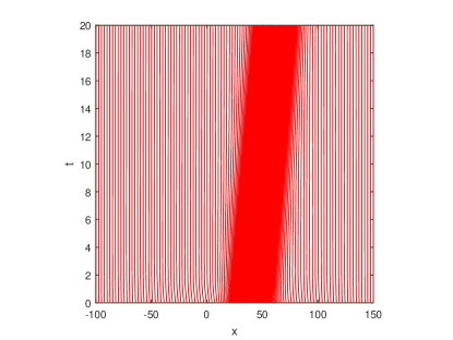
The error and convergence order are listed in Table 1 for both fixed and moving meshes. It can be seen that while both types of mesh lead to the same second order of convergence, moving meshes produce more accurate solutions (with the error being an order of magnitude smaller) than fixed meshes. A typical numerical solution and the corresponding mesh trajectories are shown in Fig. 2. It can be seen that the mesh points are concentrated in the peak area of the soliton for the whole time, demonstrating the mesh adaptation ability of the method.
In Fig. 3(a), the difference of the conserved quantities is plotted as a function of for . Notice that for fixed and moving meshes (blue solid and dashed lines) and for the fixed mesh are indistinguishable. (In fact, they are almost at the level of roundoff error.) The difference of the conserved quantities is plotted as a function of in Fig. 3(b). We can see that for both fixed and moving meshes and for moving meshes are quite significant for relatively small . However, decreases quickly to the level of roundoff error as increases for both fixed and moving meshes. On the other hand, with fixed meshes remains very small for the considered range of , consistent with the fact that is conserved on a fixed mesh by the semi-discrete system of the method. With moving meshes, is much bigger, reflecting the fact that is not conserved by the method on moving meshes. Nevertheless, it decreases at a rate , much faster than the first order predicted in (24). Thus far we have seen that this example the fixed mesh method has better conservation properties than the moving mesh method but gives less accurate solutions. It could be interesting to explore what advantages the conservation of the quantities gives to the scheme for the RLW equation.
| Moving Mesh | Fixed Mesh | |||||||
|---|---|---|---|---|---|---|---|---|
| error | order | error | order | error | order | error | order | |
| 20 | 2.62E-1 | 1.09E-1 | 4.86E-0 | 1.28E-0 | ||||
| 40 | 5.44E-2 | 2.27 | 2.04E-2 | 2.42 | 1.57E-0 | 1.63 | 5.94E-1 | 1.11 |
| 80 | 1.29E-2 | 2.08 | 4.51E-3 | 2.17 | 3.34E-1 | 2.17 | 1.82E-1 | 1.71 |
| 160 | 3.15E-3 | 2.03 | 1.08E-3 | 2.07 | 7.86E-2 | 2.14 | 4.75E-2 | 1.94 |
| 320 | 7.84E-4 | 2.01 | 2.66E-4 | 2.02 | 1.91E-2 | 2.04 | 1.93E-2 | 1.99 |
| 640 | 1.96E-4 | 2.00 | 6.23E-5 | 2.00 | 4.76E-3 | 2.01 | 2.98E-3 | 2.00 |
(a): Computed solution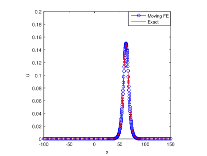 (b): Mesh trajectories
(a)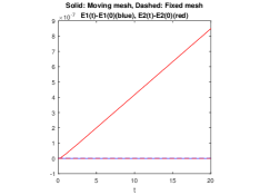 (b)
(b)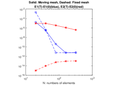
Example 4.2.
(1D RLW with interaction of two solitary waves) In this example, we study the interaction of two solitary waves for the 1D RLW equation (33) with a homogeneous Dirichlet boundary condition and the initial condition
where , , , , , , and . Initially, the solitons have the amplitude and location () and the larger soliton is placed on the left of the smaller one. An interaction occurs as the larger one is catching up with and eventually passes the smaller one. The simulation is performed on a domain until . The exact analytical solution is unavailable for this example.
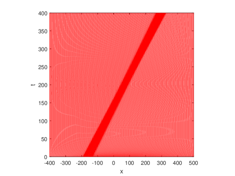
A numerical solution at and the mesh trajectories are shown in Fig. 4. The interaction of the two solitons can be clearly seen from the figure. Moreover, the width of the mesh concentration also changes with time, becoming narrower during the interaction. For comparison purpose, the solutions obtained with fixed meshes of and are plotted in Fig. 5. Oscillations are visible along the -axis in the solution with the fixed mesh of . The differences, and , are plotted as functions of in Fig. 6. Once again, for fixed and moving meshes and for moving meshes are significant for small . drops quickly as increases for both fixed and moving meshes. On the other hand, stays very small for fixed meshes. It is relatively large for moving meshes although it decreases at a rate of about , which is faster than what indicated by (24).
(a) Computed solution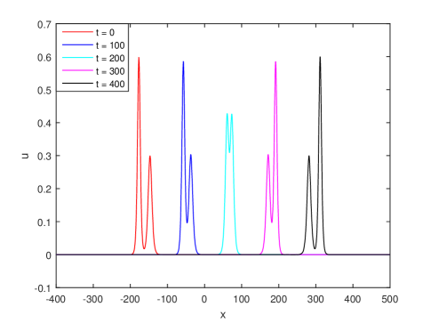 (b): Mesh trajectories
(a) Computed solution with 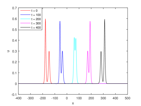 (b) Computed solution with
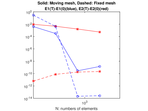
and are plotted as functions of .
Example 4.3.
(1D RLW with undular bore) We consider the development of an undular bore (e.g., see [38]) for the 1D RLW equation (33) with the initial condition
where , , , , and or . The boundary condition is at (upstream) and at (downstream). In this example, can be thought as the water depth above the equilibrium level and as the slope between the still water and deeper water. The computation is done until . Due to the continuous injection at the left boundary and the finite propagation velocity, the undular bore forms and then is expanding its range as time evolves.
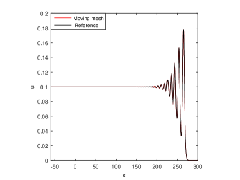
Numerical solutions at and mesh trajectories with are shown in Fig. 7 for fixed and moving meshes. A solution obtained with the fixed mesh of is used as the reference solution. It can be seen that the solution obtained with a moving mesh is more accurate than that with a fixed mesh of the same number of elements and the mesh concentration reflects correctly the development of the undular bore. The quantities and are plotted in Fig. 8. As the water coming from the left boundary at a constant rate, these quantities grow linearly with time. Nevertheless, remains very small, almost indistinguishable from the -axis. (Recall that the error in preserving on a moving mesh is at the level of roundoff error for a sufficiently fine mesh.) Finally, numerical results show that the undular bore is very stable.
(a) (fixed mesh)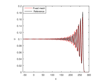 (b) (moving mesh)
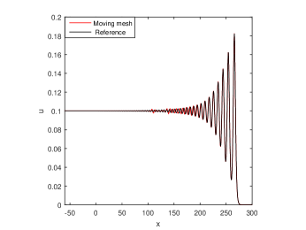 (c)
(c) 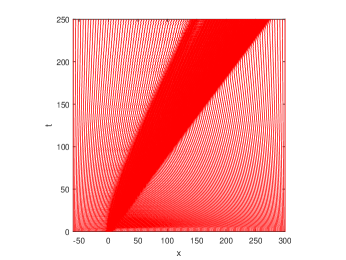 (d) (fixed mesh)
 (e) (moving mesh)
 (f)
(f) 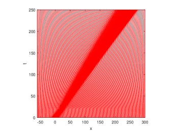
(a) 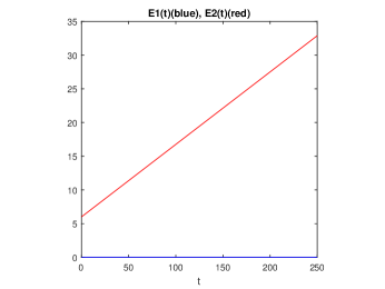 (b)
(b) 
Example 4.4.
(1D modified RLW with the Maxwellian initial condition) In this test, we consider the 1D modified RLW (MRLW) equation
subject to a homogeneous Dirichlet boundary condition and the Maxwellian initial condition [17]
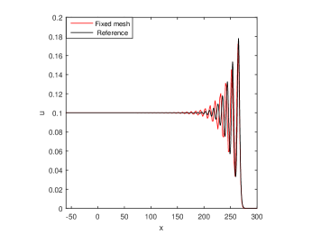
We take and or . For the time being, the Maxwellian initial condition develops into a train of solitary waves, with the wave number and amplitude depending on the value of . The smaller is, the more solitary waves will form.
The computation is performed with and . Numerical results obtained with fixed and moving meshes are shown in Fig. 9. It can be seen that the solution with a moving mesh is more accurate than that with a fixed mesh and, indeed, the former is almost indistinguishable from the reference solution which is obtained with a fixed mesh of . Numerical experiment also shows that the train of the solitons are stable.
(a): (fixed mesh)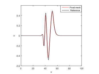 (b): (moving mesh)
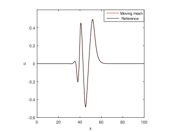 (c):
(c): 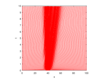 (d): (fixed mesh)
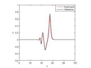 (e): (moving mesh)
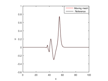 (f):
(f): 
Example 4.5.
(2D RLW with two solitary waves) In this test we consider the 2D RLW equation (1) with . The Dirichlet and initial conditions are chosen such that the exact solution is given by
where , , , , , , , and . Notice that is the maximum amplitude and is the circular frequency. The computation is performed on with .
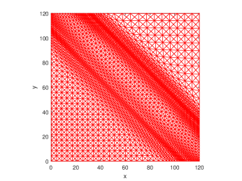
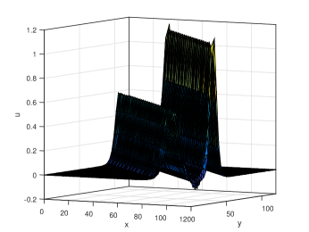
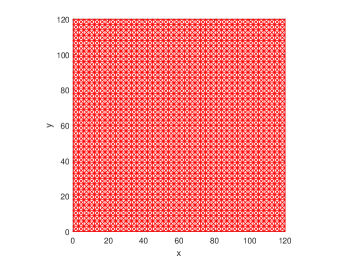
Numerical results are shown in Table 2 and Fig. 10. They indicate that the finite element method is second order for both fixed and moving meshes. Moreover, a moving mesh leads to more accurate solutions, with roughly an order of magnitude smaller error, than a fixed mesh of the same number of elements.
| Moving Mesh | Fixed Mesh | |||||||
|---|---|---|---|---|---|---|---|---|
| error | order | error | order | error | order | error | order | |
| 100 | 3.59E-1 | 1.73E1 | 3.84E-1 | 1.77E1 | ||||
| 400 | 1.02E-1 | 1.82 | 4.87E-0 | 1.82 | 2.77E-1 | 0.47 | 1.19E1 | 0.56 |
| 1600 | 1.45E-2 | 2.81 | 1.02E-0 | 2.25 | 1.32E-1 | 1.07 | 6.72E-0 | 0.83 |
| 6400 | 2.82E-3 | 2.36 | 1.97E-1 | 2.38 | 3.45E-2 | 1.93 | 2.20E-0 | 1.61 |
| 25600 | 6.24E-4 | 2.18 | 4.18E-2 | 2.24 | 8.34E-3 | 2.05 | 6.11E-1 | 1.85 |
(a): On moving mesh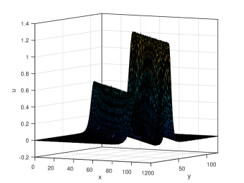 (b): Moving mesh
 (c): On fixed mesh
 (d): Fixed mesh
Example 4.6.
(2D RLW with undular bore) This example is a two-dimensional generalization of Example 4.3 (the 1D undular bore). The equation (1) is subject to a homogeneous Dirichlet boundary condition and the initial condition
where , , , , , and . The computation is performed on with .
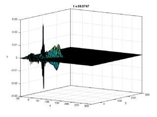
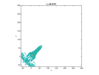
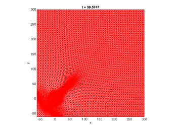
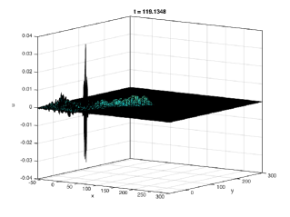
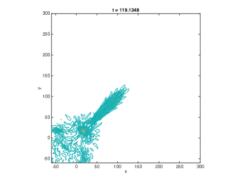
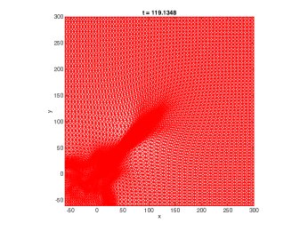
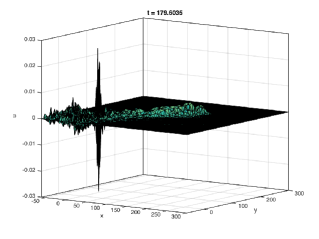
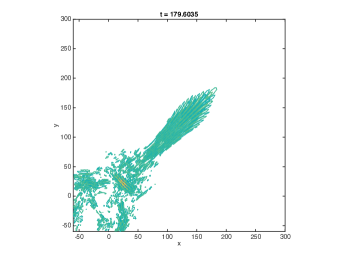
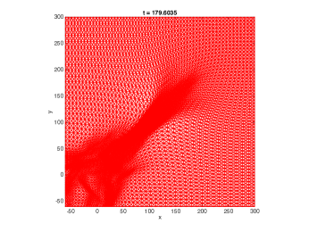
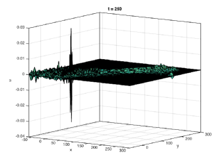
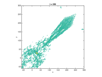
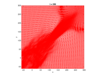
Fig. 11 shows the development and expansion of the 2D undular bore which propagates in a northeast direction. Compared to the 1D situation, the propagation is slightly slower and the amplitude is smaller. The mesh concentration correctly reflects the development of the undular bore.
Example 4.7.
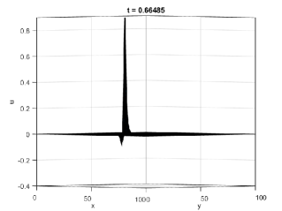
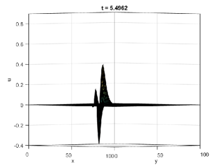
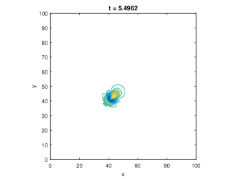
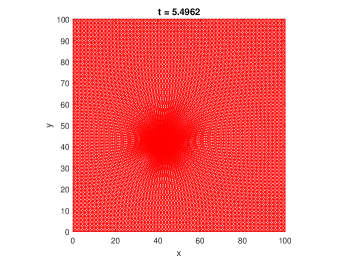
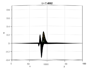
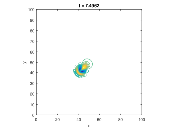
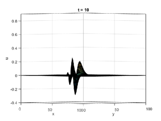
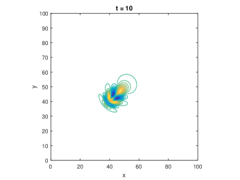
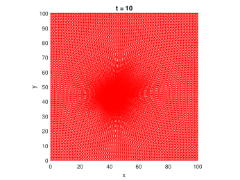
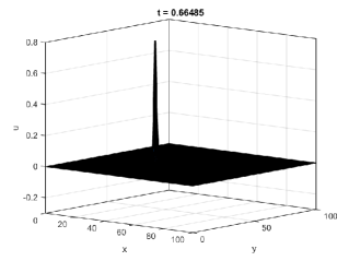
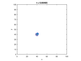
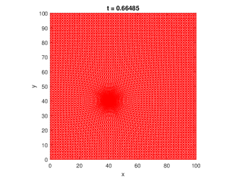
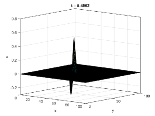
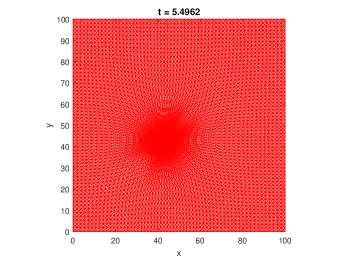
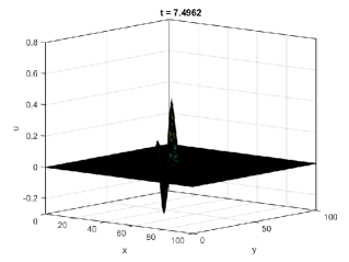
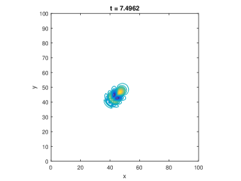
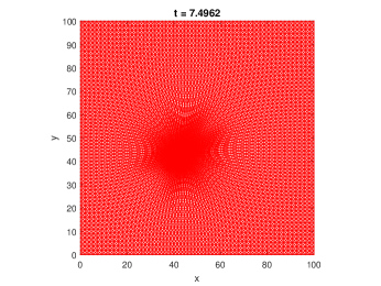
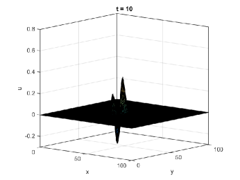
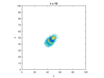
(2D RLW with the Maxwellian initial condition) In this final example, we consider the initial Maxwellian initial condition
for the 2D MRLW equation
where , and or . A homogeneous Dirichlet boundary condition is used. The computation is performed on with .





5 Conclusions and further comments
In the previous sections we have studied an adaptive moving mesh finite element method for the numerical solution of the RLW equation. The RLW equation represents a class of PDEs containing spatial-time mixed derivatives. For the numerical solution of those PDEs, a finite element method cannot be applied on a moving mesh since the mixed derivatives of the finite element approximation may not be defined. To avoid this difficulty, a new variable (2) was introduced and the RLW equation was rewritten into a system of two coupled PDEs. The system was then discretized in space using linear finite elements on a moving mesh which is generated with a new implementation of the moving mesh PDE method. The ODE system was integrated in time using the fifth-order Radau IIA scheme.
A range of numerical examples in one and two dimensions were presented. They include the RLW equation with one or two solitary waves and special initial conditions that lead to the undular bore and solitary train solutions. Numerical results have demonstrated that the moving mesh finite element method has a second order convergence as the mesh is being refined and is able to move and adapt the mesh to the evolving features in the solution of the RLW equation. Moreover, the method produces an error an order of magnitude smaller than that with a fixed mesh of the same number of elements.
It should be mentioned that the finite element approximation with both fixed and moving meshes does not preserve (the mass) but the error quickly decreases to the level of roundoff error as the mesh is refined. On the other hand, the moving mesh finite element method does a worse job to conserve (the energy) than the fixed mesh finite element method although the former is more accurate. It would be interesting to know what advantages the conservation of this quantity may give the scheme for the RLW equation. A major difficulty for the moving mesh method to conserve comes from the mesh movement, which makes the mass matrix time dependent and introduces an extra convection term (see (13)). How to design a moving mesh method that conserves this quantity will also be an interesting research topic.
Acknowledgment. The work was partially supported by NSFC through grants 91230110, 11571290, and 41375115. The authors are grateful to the anonymous referee for the valuable comments in improving the quality of the paper.
References
- [1] K. O. Abdulloev, I. L. Bogolubsky, and V. G. Makhankov. One more example of inelastic soliton interaction. Phys. Lett. A, 56:427–428, 1976.
- [2] J. Avrin and J. A. Goldstein. Global existence for the Benjamin-Bona-Mahony equation in arbitrary dimensions. Nonlinear Anal., 9:861–865, 1985.
- [3] M. J. Baines. Moving Finite Elements. Oxford University Press, Oxford, 1994.
- [4] M. J. Baines, M. E. Hubbard, and P. K. Jimack. Velocity-based moving mesh methods for nonlinear partial differential equations. Commun. Comput. Phys., 10:509–576, 2011.
- [5] T. B. Benjamin, J. L. Bona, and J. J. Mahony. Model equations for long waves in nonlinear dispersive systems. Phil. Trans. Royal Soc. London, A 227:47–78, 1972.
- [6] J. L. Bona, W. R. McKinney, and J. M. Restrepo. Stable and unstable solitary-wave solutions of the generalized regularized long-wave equation. J. Nonl. Sci., 10:603–638, 2000.
- [7] J. L. Bona, W. G. Pritchard, and L. R. Scott. An evaluation of a model equation for water waves. Phil. Trans. Royal Soc. London, A 302:457–510, 1981.
- [8] C. J. Budd, W. Huang, and R. D. Russell. Adaptivity with moving grids. Acta Numerica, 18:111–241, 2009.
- [9] F. Calogero and A. Degasperis. Spectral Transform and Solitons: Tools to Solve and Investigate Nonlinear Evolution Equations. North-Holland, New York, 1982.
- [10] B. Calvert. The equation . Math. Proc. Cambridge Philos. Soc., 79:545–561, 1976.
- [11] İ. Daǧ, B. Saka, and D. Irk. Application of cubic B-splines for numerical solution of the RLW equation. Appl. Math. Comput., 159:373–389, 2004.
- [12] M. Dehghan and R. Salehi. The solitary wave solution of the two-dimensional regularized long-wave equation in fluids and plasmas. Comput. Phys. Comm., 182:2540–2549, 2011.
- [13] A. Dogan. Numerical solution of RLW equation using linear finite elements within Galerkin’s method. Appl. Math. Modeling, 26:771–783, 2002.
- [14] J. C. Eilbeck and G. R. McGuire. Numerical study of the regularized long-wave equation I: Nnumerical methods. J. Comput. Phys., 19:43–57, 1975.
- [15] J. C. Eilbeck and G. R. McGuire. Numerical study of the regularized long-wave equation II: Iinteraction of solitary waves. J. Comput. Phys., 23:63–73, 1975.
- [16] F. Gao, J. Qiu, and Q. Zhang. Local discontinuous Galerkin finite element method and error estimates for one class of Sobolev equation. J. Sci. Comput., 41:436–460, 2009.
- [17] Y. Gao and L. Mei. Mixed Galerkin finite element methods for modified regularized long wave equation. Appl. Math. Comp., 258:267–281, 2015.
- [18] J. A. Goldstein and B. J. Wichnoski. On the Benjamin-Bona-Mahony equation in higher dimensions. Nonlinear Anal., 4:665–675, 1980.
- [19] S. González-Pinto, J. I. Montijano, and S. Pérez-Rodríguez. Two-step error estimators for implicit Runge-Kutta methods applied to stiff systems. ACM Trans. Math. Software, 30(1):1–18, 2004.
- [20] H. Gu and N. Chen. Least-squares mixed finite element methods for the RLW equations. Numer. Meth. P.D.E, 24:749–758, 2008.
- [21] B.-Y. Guo and W.-M. Cao. The fourier pseudospectral method with a restrain operator for the RLW equation. J. Comput. Phys., 74:110–126, 1988.
- [22] E. Hairer and G. Wanner. Solving Ordinary Differential Equations. II, volume 14 of Springer Series in Computational Mathematics. Springer-Verlag, Berlin, second edition, 1996. Stiff and differential-algebraic problems.
- [23] W. Huang. Variational mesh adaptation: isotropy and equidistribution. J. Comput. Phys., 174:903–924, 2001.
- [24] W. Huang. Mathematical principles of anisotropic mesh adaptation. Comm. Comput. Phys., 1:276–310, 2006.
- [25] W. Huang and L. Kamenski. A geometric discretization and a simple implementation for variational mesh generation and adaptation. J. Comput. Phys., 301:322–337, 2015. (arXiv:1410.7872).
- [26] W. Huang and L. Kamenski. On the mesh nonsingularity of the moving mesh PDE method. submitted, 2015. (arXiv:1512.04971).
- [27] W. Huang, Y. Ren, and R. D. Russell. Moving mesh methods based on moving mesh partial differential equations. J. Comput. Phys., 113:279–290, 1994.
- [28] W. Huang, Y. Ren, and R. D. Russell. Moving mesh partial differential equations (MMPDEs) based upon the equidistribution principle. SIAM J. Numer. Anal., 31:709–730, 1994.
- [29] W. Huang and R. D. Russell. Adaptive Moving Mesh Methods. Springer, New York, 2011. Applied Mathematical Sciences Series, Vol. 174.
- [30] W. Huang and W. Sun. Variational mesh adaptation II: error estimates and monitor functions. J. Comput. Phys., 184:619–648, 2003.
- [31] P. K. Jimack and A. J. Wathen. Temporal derivatives in the finite-element method on continuously deforming grids. SIAM J. Numer. Anal., 28:990–1003, 1991.
- [32] L. Kamenski and W. Huang. How a nonconvergent recovered Hessian works in mesh adaptation. SIAM J. Numer. Anal., 52:1692–1708, 2014. (arXiv:1211.2877).
- [33] Z. Luo and R. Liu. Mixed finite element analysis and numerical solitary solution for the RLW equation. SIAM J. Numer. Anal., 36:89–104 (electronic), 1999.
- [34] W. X. Ma and B. Fuchssteiner. Explicit and exact solutions to a Kolmogorov-Petrovskii-Piskunov equation. I. J. Non-Linear Mech., 31:329–338, 1996.
- [35] V. B. Matveev and M. A. Salle. Darboux Transformations and Solitons. Springer-Verlag, 1991.
- [36] L. A. Medeiros and M. M. Miranda. Weak solutions for a nonlinear dispersive equation. J. Math. Anal.Appl., 59:432–441, 1977.
- [37] L. Mei and Y. Chen. Explicit multistep method for the numerical solution of RLW equation. Appl. Math. Comput., 218:9547–9554, 2012.
- [38] L. Mei and Y. Chen. Numerical solutions of RLW equation using Galerkin method with extrapolation techniques. Comput. Phys. Comm., 183:1609–1616, 2012.
- [39] L. Mei, Y. Gao, and Z. Chen. Numerical study using explicit multistep Galerkin finite element method for the MRLW equation. Numer. Meth. P.D.E., 31:1875–1889, 2015.
- [40] P. J. Olver. Euler operators and conservation laws of the BBM equation. Math. Proc. Cambridge Phil. Soc., 85:143–160, 1979.
- [41] D. H. Peregrine. Calculations of the development of an undular bore. J. Fluid Mech., 25(2):321–330, 1966.
- [42] P. Rosenau. A quasi-continuous description of a nonlinear transmission line. Phys. Scr., 34:827–829, 1986.
- [43] R. E. Showalter. Existence and representation theorems for a semilinear Sobolev equation in Banach space. SIAM J. Math. Anal., 3:527–543, 1972.
- [44] Siraj-ul-Islam, S. Haq, and A. Ali. A meshfree method for the numerical solution of the RLW equation. J. Comput. Appl. Math., 223:997–1012, 2009.
- [45] K. Spayd and M. Shearer. The Buckley-Leverett equation with dynamic capillary pressure. SIAM J. Appl. Math., 71:1088–1108, 2011.
- [46] T. Tang. Moving mesh methods for computational fluid dynamics flow and transport. In Recent Advances in Adaptive Computation (Hangzhou, 2004), volume 383 of AMS Contemporary Mathematics, pages 141–173. Amer. Math. Soc., Providence, RI, 2005.
- [47] B. Tian, W. Li, and Y.-T. Gao. On the two-dimensional regularized long-wave equation in fluids and plasmas. Acta Mech., pages 235–239, 2003.
- [48] H. W. Yang, B. S. Yin, and Y. L. Shi. Forced dissipative Boussinesq equation for solitary waves excited by unstable topography. Nonl. Dyn., 70:1389–1396, 2012.
- [49] S. Zaki. Solitary waves of the split RLW equation. Comput. Phys. Comm., 138:80–91, 2001.