Kernel Spectral Clustering

Ilaria Giulini111The results presented in this paper were obtained while the author was preparing her PhD under the supervision of Olivier Catoni at the Département de Mathématiques et Applications, École Normale Supérieure, Paris, with the financial support of the Région Île de France.
ilaria.giulini@me.com
Abstract

We investigate the question of studying spectral clustering in a Hilbert space where the set of points to cluster are drawn i.i.d. according to an unknown probability distribution whose support is a union of compact connected components. We modify the algorithm proposed by Ng, Jordan and Weiss in [15] in order to propose a new algorithm that automatically estimates the number of clusters and we characterize the convergence of this new algorithm in terms of convergence of Gram operators. We also give a hint of how this approach may lead to learn transformation-invariant representations in the context of image classification.

Keywords. Spectral clustering, Reproducing kernel Hilbert space, Markov chain, Gram operator

1 Introduction

Clustering is the task of grouping a set of objects into classes, called clusters, in such a way that objects in the same group are more similar to each other than to those in other groups. Spectral clustering algorithms are efficiently used as an alternative to classical clustering algorithms, such as k𝑘k-means, in particular in the case of not linearly separable data sets. To perform clustering, these methods use the spectrum of some data-dependent matrices: the affinity matrix [7], or the Laplacian matrix [8]. Many different versions of spectral clustering algorithms can be found in the literature (see [12]) and one of the most successful algorithm has been proposed by Ng, Jordan and Weiss in [15]. Given a set of points to cluster into c𝑐c classes and denoting by A𝐴A the affinity matrix and by D𝐷D the diagonal matrix whose i𝑖i-th entry is the sum of the elements on the i𝑖i-th row of A𝐴A, their algorithm uses the c𝑐c largest eigenvectors of the Laplacian matrix D1/2AD1/2superscript𝐷12𝐴superscript𝐷12D^{-1/2}AD^{-1/2} simultaneously. More precisely, the data set is first embedded in a c𝑐c-dimensional space in which clusters are more evident and then points are separated using k𝑘k-means, or any other standard algorithm.
Other algorithms use different renormalizations of the affinity matrix. For example, Shi and Malik in [16] use the second smallest eigenvector of the unnormalized Laplacian matrix DA𝐷𝐴D-A to separate the data set into two groups and use the algorithm recursively to get more than two classes, whereas Meila and Shi in [14] use the first c𝑐c largest eigenvectors of the stochastic matrix D1Asuperscript𝐷1𝐴D^{-1}A (that has the same eigenvectors as the normalized Laplacian matrix ID1AIsuperscript𝐷1𝐴\mathrm{I}-D^{-1}A) to compute a partition in c𝑐c classes. These algorithms treat the question as a graph partitioning problem and they are based on the so called normalized cut criterion. Different cost functions can be found in the literature (see [6], [11]) and more generally the study of Laplacian matrices has been carry out also in different contexts, as for semi-supervised learning [5] and manifold learning [2].
We consider the setting of performing spectral clustering in a Hilbert space. This general framework includes the analysis of both data sets in a functional space and samples embedded in a reproducing kernel Hilbert space. The latter is the case of kernel methods that use the kernel trick to embed the data set into a reproducing kernel Hilbert space in order to get a new representation that simplifies the geometry of the classes. Our point of departure is the algorithm proposed by Ng, Jordan and Weiss [15] but interpreted in a infinite-dimensional setting, so that we view the matrices described above as empirical versions of some underlying integral operators. We assume that the points to cluster are drawn according to an unknown probability distribution whose support is a union of compact connected components (see [17] for consistency of clustering algorithms). Our idea is to view spectral clustering as a change of representation in a reproducing kernel Hilbert space, induced by a change of kernel, and to propose a new algorithm that automatically estimates the number of clusters. Usually the number of clusters is assumed to be know in advance (see [14], [15]) or it is linked to the presence of a sufficient large gap in the spectrum of the Laplacian matrix. To achieve our aim we replace the projection on the space spanned by the largest eigenvectors of the Laplacian matrix proposed by Ng, Jordan and Weiss with a suitable power of the Laplacian operator. Indeed, such an iteration performs some kind of soft truncation of the eigenvalues and hence leads to a natural dimensionality reduction. This iteration is related to the computation of the marginal distribution at time t𝑡t of some Markov chains with exponential rare transitions, as suggested by [4] in the case where the unknown probability distribution has a finite support. We conjecture (and this will be the subject of a future work) that the same kind of behavior holds for more general supports and we hint that spectral clustering, coupled with some preliminary change of representation in a reproducing kernel Hilbert space, can be a winning tool to bring down the representation of classes to a low-dimensional space and may lead to a generic and rather radical alternative. This suggests that the kernel trick, introduced to better separate classes in the supervised learning framework addressed by support vector machines (SVMs), is also feasible in the unsupervised context, where we do not separate classes using hyperplanes in the feature space but instead we use spectral clustering to perform the classification. We also suggest with an example how this approach may lead to learn transformation-invariant representations of a same pattern.
Developing a convincing toolbox for unsupervised invariant-shape analysis is beyond the scope of this study and it will be carried on elsewhere. However we observe that the pattern transformations we would like to take into account in image analysis are numerous and not easy to formalize: they may come from some set of transformations such as translations, rotations or scaling or they may come from the conditions in which the images have been taken, for example, changes in the perspective or in illumination, partial occlusions, object deformations, etc. Making a representation invariant with respect to a set of transformations is a challenging task even in the simpler case of translations. Indeed, it is sufficient to observe that the set of functions obtained by translating a single pattern in various directions typically spans a vector space of high dimension, meaning that the shapes (here the functions) that we would like to put in the same category do not even live in a common low-dimensional subspace. A possible approach is to study representations that leave invariant some group of transformations, for instance, the Fourier transform that has translation invariant properties, since its modulus is translation invariant. However it is unstable to small deformations at high frequencies. Wavelet transforms provide a workaround. Scattering representations proposed by Mallat [13] compute translation-invariant representations by cascading wavelet transforms and modulus pooling operators. They bring improvements for audio [1] and for image [3] classification. This kind of careful mathematical study has to be repeated for any kind of transformations. Instead of deriving the representation of a pattern from a mathematical study, the idea here is to learn the representation itself from examples of patterns that sample in a sufficiently dense way the orbits of the set of transformations at stake.
The paper is organized as follows. In Section 2 we introduce the ideal version of our algorithm that uses the underlying unknown probability distribution and we provide an interpretation of the clustering effect in terms of Markov chains. In Section 3 we introduce an empirical version of the algorithm and we provide some convergence results, based on the convergence of some Gram operators. Finally experiments are shown in Section 4.

2 The Ideal Algorithm

Let 𝒳𝒳\mathcal{X} be a compact subset of some separable Hilbert space endowed with the (unknown) probability distribution PP\mathrm{P} on 𝒳𝒳\mathcal{X} and assume that the support of PP\mathrm{P} is made of several compact connected components. Let A:𝒳×𝒳:𝐴𝒳𝒳A:\mathcal{X}\times\mathcal{X}\to\mathbb{R} be a symmetric positive semi-definite kernel, normalized in such a way that A(x,x)=1𝐴𝑥𝑥1A(x,x)=1, for any x𝑥x in the state space 𝒳𝒳\mathcal{X}, and let us define the symmetric positive semi-definite kernel

K(x,y)=A(x,y)2.𝐾𝑥𝑦𝐴superscript𝑥𝑦2K(x,y)=A(x,y)^{2}.

This kernel plays the same role of the affinity matrix, while the Laplacian matrix is now replaced by the integral operator with kernel

K¯(x,y)=μ(x)1/2K(x,y)μ(y)1/2¯𝐾𝑥𝑦𝜇superscript𝑥12𝐾𝑥𝑦𝜇superscript𝑦12\overline{K}(x,y)=\mu(x)^{-1/2}\ K(x,y)\ \mu(y)^{-1/2}

where the function

μ(x)=K(x,z)dP(z)𝜇𝑥𝐾𝑥𝑧dP𝑧\mu(x)=\int K(x,z)\mathrm{d}\mathrm{P}(z) (1)

is the analogous of the diagonal matrix D𝐷D. According to the Ng, Jordan and Weiss algorithm we consider more specifically the case where

K(x,y)=Kβ(x,y)=exp(βxy2),β>0.formulae-sequence𝐾𝑥𝑦subscript𝐾𝛽𝑥𝑦𝛽superscriptdelimited-∥∥𝑥𝑦2𝛽0K(x,y)=K_{\beta}(x,y)=\exp\bigl{(}-\beta\lVert x-y\rVert^{2}\bigr{)},\quad\beta>0.

2.1 The Algorithm

The ideal algorithm (that uses the unknown probability distribution PP\mathrm{P}) goes as follows. For any x,y𝒳,𝑥𝑦𝒳x,y\in\mathcal{X},

  1. 1.

    Form the kernel

    K¯(x,y)=μ(x)1/2K(x,y)μ(y)1/2¯𝐾𝑥𝑦𝜇superscript𝑥12𝐾𝑥𝑦𝜇superscript𝑦12\overline{K}(x,y)=\mu(x)^{-1/2}K(x,y)\mu(y)^{-1/2}

    where μ(x)=K(x,z)dP(z)𝜇𝑥𝐾𝑥𝑧dP𝑧\mu(x)=\int K(x,z)\mathrm{d}\mathrm{P}(z)

  2. 2.

    Construct the new (iterated) kernel

    K¯m(x,y)=K¯(y,z1)K¯(z1,z2)K¯(zm1,x)dP(m1)(z1,,zm1),subscript¯𝐾𝑚𝑥𝑦¯𝐾𝑦subscript𝑧1¯𝐾subscript𝑧1subscript𝑧2¯𝐾subscript𝑧𝑚1𝑥superscriptdPtensor-productabsent𝑚1subscript𝑧1subscript𝑧𝑚1\overline{K}_{m}(x,y)=\int\overline{K}(y,z_{1})\overline{K}(z_{1},z_{2})\dots\overline{K}(z_{m-1},x)\ \mathrm{d}\mathrm{P}^{\otimes(m-1)}(z_{1},\dots,z_{m-1}),

    where m>0𝑚0m>0 is a free parameter

  3. 3.

    Make a last change of kernel (normalizing the kernel K¯msubscript¯𝐾𝑚\overline{K}_{m})

    Km(x,y)=K¯2m(x,x)1/2K¯2m(x,y)K¯2m(y,y)1/2subscript𝐾𝑚𝑥𝑦subscript¯𝐾2𝑚superscript𝑥𝑥12subscript¯𝐾2𝑚𝑥𝑦subscript¯𝐾2𝑚superscript𝑦𝑦12K_{m}(x,y)=\overline{K}_{2m}(x,x)^{-1/2}\ \overline{K}_{2m}(x,y)\ \overline{K}_{2m}(y,y)^{-1/2}
  4. 4.

    Cluster points according to the new representation defined by the kernel Kmsubscript𝐾𝑚K_{m}.

As it is suggested in the next section, the representation induced by the kernel Kmsubscript𝐾𝑚K_{m} makes the subsequent classification an easy task.

2.2 The Clustering Effect

The main idea is that, in the Hilbert space defined by the kernel Kmsubscript𝐾𝑚K_{m}, clusters are concentrated around orthogonal unit vectors, forming the vertices of a regular simplex. To give an intuition of this clustering effect, we provide a Markov chain analysis of the algorithm, according to some ideas suggested by [4].
Assume that the scale parameter β𝛽\beta in the Gaussian kernel K𝐾K is large enough. For the choice of β𝛽\beta we refer to Section 2.3.
Define the kernel

M(x,y)=μ(x)1K(x,y)𝑀𝑥𝑦𝜇superscript𝑥1𝐾𝑥𝑦M(x,y)=\mu(x)^{-1}K(x,y)

where μ𝜇\mu is defined in  equation 1 and consider the corresponding integral operator

𝐌(f):xM(x,z)f(z)dP(z).:𝐌𝑓maps-to𝑥𝑀𝑥𝑧𝑓𝑧dP𝑧\mathbf{M}(f):x\mapsto\int M(x,z)f(z)\,\mathrm{d}\mathrm{P}(z).

Observe that 𝐌𝐌\mathbf{M} is the transition operator of a Markov chain (Zk)ksubscriptsubscript𝑍𝑘𝑘(Z_{k})_{k\in\mathbb{N}} on 𝒳𝒳\mathcal{X} and that

M(x,y)=dZ1|Z0=xdP(y).𝑀𝑥𝑦dsubscriptconditionalsubscript𝑍1subscript𝑍0𝑥dP𝑦M(x,y)=\frac{\mathrm{d}\mathbb{P}_{Z_{1}|Z_{0}=x}}{\mathrm{d}\mathrm{P}}(y).

So the Markov chain related to the operator 𝐌𝐌\mathbf{M} has a small probability to jump from one component to another one. As already said, from  [4] it can be deduced that, when the support of PP\mathrm{P} is finite, for suitable values of m𝑚m, depending on β𝛽\beta as exp(βT2)𝛽superscript𝑇2\exp(\beta T^{2}), the measure

𝐌xm:f𝐌m(f)(x):superscriptsubscript𝐌𝑥𝑚maps-to𝑓superscript𝐌𝑚𝑓𝑥\mathbf{M}_{x}^{m}:f\mapsto\mathbf{M}^{m}(f)(x)

is close (for large enough values of β𝛽\beta) to be supported by a cycle of depth larger than H𝐻H of the state space. The cycle decomposition of the state space of a Markov chain with exponential transitions is some discrete counterpart of the decomposition into connected components. More precisely, the measure 𝐌xmsuperscriptsubscript𝐌𝑥𝑚\mathbf{M}_{x}^{m} is close to the invariant measure of the operator 𝐌𝐌\mathbf{M} restricted to the connected component which x𝑥x belongs to. As a result, the function x𝐌m(f)(x)maps-to𝑥superscript𝐌𝑚𝑓𝑥x\mapsto\mathbf{M}^{m}(f)(x) is approximately constant on each connected component. Thus, for reasons that we will not try to prove here, but that are confirmed by experiments, we expect the same kind of behaviour in the general setting. To rewrite this conjecture in terms of the kernel Kmsubscript𝐾𝑚K_{m} we introduce the following proposition.

Proposition 1.

Let QQ\mathrm{Q} be the invariant measure of the Markov transition operator 𝐌𝐌\mathbf{M} and define

x=μ(x)1/2d𝐌xmdQLQ2,x𝒳.formulae-sequencesubscript𝑥𝜇superscript𝑥12dsubscriptsuperscript𝐌𝑚𝑥dQsubscriptsuperscript𝐿2Q𝑥𝒳\mathfrak{R}_{x}=\mu(x)^{1/2}\frac{\mathrm{d}\mathbf{M}^{m}_{x}}{\mathrm{d}\mathrm{Q}}\in L^{2}_{\mathrm{Q}},\qquad x\in\mathcal{X}.

It holds that

Km(x,y)=xxLQ2,yyLQ2LQ2.subscript𝐾𝑚𝑥𝑦subscriptsubscript𝑥subscriptdelimited-∥∥subscript𝑥subscriptsuperscript𝐿2Qsubscript𝑦subscriptdelimited-∥∥subscript𝑦subscriptsuperscript𝐿2Qsubscriptsuperscript𝐿2QK_{m}(x,y)=\Bigl{\langle}\frac{\mathfrak{R}_{x}}{\lVert\mathfrak{R}_{x}\rVert_{L^{2}_{\mathrm{Q}}}},\frac{\mathfrak{R}_{y}}{\lVert\mathfrak{R}_{y}\rVert_{L^{2}_{\mathrm{Q}}}}\Bigr{\rangle}_{L^{2}_{\mathrm{Q}}}.
Proof.

Using the fact that K¯=K¯1¯𝐾subscript¯𝐾1\overline{K}=\overline{K}_{1} and that

K¯m(x,y)=K¯(x,z)K¯m1(z,y)dP(z),subscript¯𝐾𝑚𝑥𝑦¯𝐾𝑥𝑧subscript¯𝐾𝑚1𝑧𝑦dP𝑧\overline{K}_{m}(x,y)=\int\overline{K}(x,z)\overline{K}_{m-1}(z,y)\,\mathrm{d}\mathrm{P}(z), (2)

by induction we get

𝐌m(f)(x)=μ(x)1/2K¯m(x,z)μ(z)1/2f(z)dP(z).superscript𝐌𝑚𝑓𝑥𝜇superscript𝑥12subscript¯𝐾𝑚𝑥𝑧𝜇superscript𝑧12𝑓𝑧dP𝑧\mathbf{M}^{m}(f)(x)=\mu(x)^{-1/2}\int\overline{K}_{m}(x,z)\mu(z)^{1/2}f(z)\,\mathrm{d}\mathrm{P}(z).

Thus the measure 𝐌xmsubscriptsuperscript𝐌𝑚𝑥\mathbf{M}^{m}_{x} has density

d𝐌xmdP(y)=μ(x)1/2K¯m(x,y)μ(y)1/2.dsubscriptsuperscript𝐌𝑚𝑥dP𝑦𝜇superscript𝑥12subscript¯𝐾𝑚𝑥𝑦𝜇superscript𝑦12\frac{\mathrm{d}\mathbf{M}^{m}_{x}}{\mathrm{d}\mathrm{P}}(y)=\mu(x)^{-1/2}\overline{K}_{m}(x,y)\ \mu(y)^{1/2}.

Moreover, since

μ(x)M(x,y)f(y)dP(x)dP(y)=K(x,y)f(y)dP(x)dP(y)=μ(y)f(y)dP(y),𝜇𝑥𝑀𝑥𝑦𝑓𝑦dP𝑥dP𝑦𝐾𝑥𝑦𝑓𝑦dP𝑥dP𝑦𝜇𝑦𝑓𝑦dP𝑦\int\mu(x)M(x,y)f(y)\,\mathrm{d}\mathrm{P}(x)\mathrm{d}\mathrm{P}(y)=\int K(x,y)f(y)\,\mathrm{d}\mathrm{P}(x)\mathrm{d}\mathrm{P}(y)=\int\mu(y)f(y)\,\mathrm{d}\mathrm{P}(y),

the invariant measure QQ\mathrm{Q} has a density with respect to PP\mathrm{P} equal to dQdP=μ.dQdP𝜇\frac{\mathrm{d}\mathrm{Q}}{\mathrm{d}\mathrm{P}}=\mu. As a consequence

d𝐌xmdQ(y)=μ(x)1/2K¯m(x,y)μ(y)1/2.dsubscriptsuperscript𝐌𝑚𝑥dQ𝑦𝜇superscript𝑥12subscript¯𝐾𝑚𝑥𝑦𝜇superscript𝑦12\frac{\mathrm{d}\mathbf{M}^{m}_{x}}{\mathrm{d}\mathrm{Q}}(y)=\mu(x)^{-1/2}\overline{K}_{m}(x,y)\ \mu(y)^{-1/2}.

According to  equation 2 and recalling the definition of Kmsubscript𝐾𝑚K_{m} we conclude the proof. \blacksquare

With these definitions, our conjecture can be formulated as

limβKexp(βT2)(x,y)=C𝒞T𝟙({x,y}C),subscript𝛽subscript𝐾𝛽superscript𝑇2𝑥𝑦subscript𝐶subscript𝒞𝑇1𝑥𝑦𝐶\lim_{{\beta}\to\infty}K_{\exp({\beta}T^{2})}(x,y)=\sum_{C\in\mathcal{C}_{T}}\mathbbm{1}\left(\{x,y\}\subset C\right),

where 𝒞Tsubscript𝒞𝑇\mathcal{C}_{T} denotes the connected components of the graph {x,ysupp(P)|yx<T}.conditional-set𝑥𝑦suppPnorm𝑦𝑥𝑇\left\{x,y\in\mathrm{supp}(\mathrm{P})\ |\ \|y-x\|<T\right\}. Remark that, as we assumed that the support of PP\mathrm{P} is a union of compact topological connected components, taking T𝑇T to be less than the minimum distance between two topological components of supp(P)suppP\operatorname{\mathrm{supp}}(\mathrm{P}), we obtain that 𝒞Tsubscript𝒞𝑇\mathcal{C}_{T} coincides with the topological components of supp(P)suppP\operatorname{\mathrm{supp}}(\mathrm{P}). As a consequence, for suitable values of the scale parameter β𝛽\beta and of the number of iterations m𝑚m, the kernel Km(x,y)subscript𝐾𝑚𝑥𝑦K_{m}(x,y) is close to zero (or equivalently the supports of the probability measures 𝐌xmsubscriptsuperscript𝐌𝑚𝑥\mathbf{M}^{m}_{x} and 𝐌ymsubscriptsuperscript𝐌𝑚𝑦\mathbf{M}^{m}_{y} are almost disjoint) if x𝑥x and y𝑦y belong to two different clusters, whereas it is close to one (or equivalently the supports of 𝐌xmsubscriptsuperscript𝐌𝑚𝑥\mathbf{M}^{m}_{x} and 𝐌ymsubscriptsuperscript𝐌𝑚𝑦\mathbf{M}^{m}_{y} are almost the same) when x𝑥x and y𝑦y belong to the same cluster. Moreover since the kernel Km(x,y)subscript𝐾𝑚𝑥𝑦K_{m}(x,y) is the cosine of the angle formed by the two vectors representing x𝑥x and y𝑦y, according to the conjecture, it is either close to zero or close to one, showing that, in the Hilbert space defined by Kmsubscript𝐾𝑚K_{m}, clusters are concentrated around orthogonal unit vectors.

2.3 Choice of the Scale Parameter

We conclude this section with some remarks on the choice of the scale parameter β.𝛽\beta. In the case where the influence kernel K𝐾K is of the form

K(x,y)=Kβ(x,y)=exp(βxy2),𝐾𝑥𝑦subscript𝐾𝛽𝑥𝑦𝛽superscriptdelimited-∥∥𝑥𝑦2K(x,y)=K_{\beta}(x,y)=\exp\bigl{(}-\beta\lVert x-y\rVert^{2}\bigr{)},

we propose to choose β𝛽\beta as the solution of the equation

F(β):=Kβ(x,y)2dP(x)dP(y)=hassign𝐹𝛽subscript𝐾𝛽superscript𝑥𝑦2dP𝑥dP𝑦F(\beta):=\int K_{\beta}(x,y)^{2}\,\mathrm{d}\mathrm{P}(x)\mathrm{d}\mathrm{P}(y)=h

where hh is a suitable parameter which measures the probability that two independent points drawn according to the probability PP\mathrm{P} are close to each other. Introducing the Gram operator Lβ:LP2LP2:subscript𝐿𝛽subscriptsuperscript𝐿2Psubscriptsuperscript𝐿2PL_{\beta}:L^{2}_{\mathrm{P}}\to L^{2}_{\mathrm{P}} defined by the kernel Kβsubscript𝐾𝛽K_{\beta} as

Lβ(f)(x)=Kβ(x,y)f(y)dP(y),x𝒳,formulae-sequencesubscript𝐿𝛽𝑓𝑥subscript𝐾𝛽𝑥𝑦𝑓𝑦dP𝑦𝑥𝒳L_{\beta}(f)(x)=\int K_{\beta}(x,y)f(y)\,\mathrm{d}\mathrm{P}(y),\quad x\in\mathcal{X},

the parameter hh is equal to the square of the Hilbert-Schmidt norm of Lβ.subscript𝐿𝛽L_{\beta}. Observe that Lβsubscript𝐿𝛽L_{\beta} has a discrete spectrum λ1λ20subscript𝜆1subscript𝜆20\lambda_{1}\geq\lambda_{2}\geq\dots\geq 0 that satisfies, according to the Mercer theorem,

i=1+λisuperscriptsubscript𝑖1subscript𝜆𝑖\displaystyle\sum_{i=1}^{+\infty}\lambda_{i} =Kβ(x,x)dP(x)=1,absentsubscript𝐾𝛽𝑥𝑥dP𝑥1\displaystyle=\int K_{\beta}(x,x)\,\mathrm{d}\mathrm{P}(x)=1,
i=1+λi2superscriptsubscript𝑖1superscriptsubscript𝜆𝑖2\displaystyle\sum_{i=1}^{+\infty}\lambda_{i}^{2} =F(β)1absent𝐹𝛽1\displaystyle=F(\beta)\leq 1

since Kβ(x,x)=1subscript𝐾𝛽𝑥𝑥1K_{\beta}(x,x)=1. We also observe that

limβ0F(β)=1subscript𝛽0𝐹𝛽1\lim_{\beta\rightarrow 0}F(\beta)=1

which implies that for β𝛽\beta going to zero, λ1subscript𝜆1\lambda_{1} goes to one whereas all the other eigenvalues λisubscript𝜆𝑖\lambda_{i}, for i2𝑖2i\geq 2, go to zero. Moreover,

limβ+F(β)=0,subscript𝛽𝐹𝛽0\lim_{\beta\rightarrow+\infty}F(\beta)=0,

so that when β𝛽\beta grows, the eigenvalues are spread more and more widely. Therefore, F(β)𝐹𝛽F(\beta) governs the spread of the eigenvalues of Lβsubscript𝐿𝛽L_{\beta}. For these reasons, the value of the parameter h=F(β)𝐹𝛽h=F(\beta) controls the effective dimension of the representation of the distribution of points PP\mathrm{P} in the reproducing kernel Hilbert space defined by Kβsubscript𝐾𝛽K_{\beta}. Experiments show that this effective dimension has to be pretty large in order to have a proper clustering effect, meaning that we will impose a small value of the parameter hh.
Note that in the experiments we do not have access to the function F(β)𝐹𝛽F(\beta) but we have to consider its empirical version

1n(n1)1i<jnKβ(Xi,Xj)21𝑛𝑛1subscript1𝑖𝑗𝑛subscript𝐾𝛽superscriptsubscript𝑋𝑖subscript𝑋𝑗2\frac{1}{n(n-1)}\sum_{1\leq i<j\leq n}K_{\beta}(X_{i},X_{j})^{2}

where X1,,Xnsubscript𝑋1subscript𝑋𝑛X_{1},\dots,X_{n} is an i.i.d. sample drawn from the probability distribution PP\mathrm{P}.

3 The Empirical Algorithm

In order to provide an empirical version of the ideal algorithm proposed in Section 2, we connect the previous kernels with some Gram operators. Note that by empirical algorithm we mean an algorithm based on the sample distribution instead of on the unknown probability distribution PP\mathrm{P}.
From now on, given a Hilbert space 𝒦𝒦\mathcal{K} and a probability distribution 𝒫𝒫\mathcal{P} on 𝒦𝒦\mathcal{K}, the Gram operator 𝔊:𝒦𝒦:𝔊𝒦𝒦\mathfrak{G}:\mathcal{K}\to\mathcal{K} is defined as

𝔊u=𝔼Y𝒫[u,Y𝒦Y].𝔊𝑢subscript𝔼similar-to𝑌𝒫delimited-[]subscript𝑢𝑌𝒦𝑌\mathfrak{G}u=\mathbb{E}_{Y\sim\mathcal{P}}\big{[}\langle u,Y\rangle_{\mathcal{K}}\ Y\big{]}.

The next proposition links the function μ𝜇\mu defined in  equation 1 to the Gram operator defined in the reproducing kernel Hilbert space induced by the kernel

A(x,y)=K(x,y)1/2=exp(βxy2/2).𝐴𝑥𝑦𝐾superscript𝑥𝑦12𝛽superscriptnorm𝑥𝑦22A(x,y)=K(x,y)^{1/2}=\exp\left(-\beta\|x-y\|^{2}/2\right).
Proposition 2.

Let Asubscript𝐴\mathcal{H}_{A} be the reproducing kernel Hilbert space defined by A𝐴A and ϕA:𝒳A:subscriptitalic-ϕ𝐴𝒳subscript𝐴\phi_{A}:\mathcal{X}\to\mathcal{H}_{A} the corresponding feature map. Denote by 𝒢A:AA:subscript𝒢𝐴subscript𝐴subscript𝐴\mathcal{G}_{A}:\mathcal{H}_{A}\to\mathcal{H}_{A} the Gram operator

𝒢Av=v,ϕA(z)AϕA(z)dP(z).subscript𝒢𝐴𝑣subscript𝑣subscriptitalic-ϕ𝐴𝑧subscript𝐴subscriptitalic-ϕ𝐴𝑧dP𝑧\mathcal{G}_{A}v=\int\langle v,\phi_{A}(z)\rangle_{\mathcal{H}_{A}}\ \phi_{A}(z)\,\mathrm{d}\mathrm{P}(z).

Then

μ(x)=ϕA(x),ϕA(z)A2dP(z)=𝒢AϕA(x),ϕA(x)A.𝜇𝑥superscriptsubscriptsubscriptitalic-ϕ𝐴𝑥subscriptitalic-ϕ𝐴𝑧subscript𝐴2dP𝑧subscriptsubscript𝒢𝐴subscriptitalic-ϕ𝐴𝑥subscriptitalic-ϕ𝐴𝑥subscript𝐴\mu(x)=\int\langle\phi_{A}(x),\phi_{A}(z)\rangle_{\mathcal{H}_{A}}^{2}\,\mathrm{d}\mathrm{P}(z)=\langle\mathcal{G}_{A}\phi_{A}(x),\phi_{A}(x)\rangle_{\mathcal{H}_{A}}.
Proof.

The result follows recalling that by the Moore-Aronszajn theorem

A(x,y)=ϕA(x),ϕA(y)A.𝐴𝑥𝑦subscriptsubscriptitalic-ϕ𝐴𝑥subscriptitalic-ϕ𝐴𝑦subscript𝐴A(x,y)=\langle\phi_{A}(x),\phi_{A}(y)\rangle_{\mathcal{H}_{A}}.

\blacksquare

A similar result relates the iterated kernel K¯msubscript¯𝐾𝑚\overline{K}_{m} to the Gram operator defined in the reproducing kernel Hilbert space induced by the Gaussian kernel K𝐾K.

Proposition 3.

Let \mathcal{H} be the reproducing kernel Hilbert space defined by K𝐾K and ϕK:𝒳:subscriptitalic-ϕ𝐾𝒳\phi_{K}:\mathcal{X}\to\mathcal{H} the corresponding feature map. Define

ϕK¯(x)=μ(x)1/2ϕK(x)subscriptitalic-ϕ¯𝐾𝑥𝜇superscript𝑥12subscriptitalic-ϕ𝐾𝑥\phi_{\overline{K}}(x)=\mu(x)^{-1/2}\phi_{K}(x) (3)

and consider the Gram operator 𝒢::𝒢\mathcal{G}:\mathcal{H}\to\mathcal{H}

𝒢v=v,ϕK¯(z)ϕK¯(z)dP(z).𝒢𝑣subscript𝑣subscriptitalic-ϕ¯𝐾𝑧subscriptitalic-ϕ¯𝐾𝑧dP𝑧\mathcal{G}v=\int\langle v,\phi_{\overline{K}}(z)\rangle_{\mathcal{H}}\ \phi_{\overline{K}}(z)\ \mathrm{d}\mathrm{P}(z). (4)

Then, for any m>0,𝑚0m>0,

K¯2m(x,y)=𝒢m1/2ϕK¯(x),𝒢m1/2ϕK¯(y).subscript¯𝐾2𝑚𝑥𝑦subscriptsuperscript𝒢𝑚12subscriptitalic-ϕ¯𝐾𝑥superscript𝒢𝑚12subscriptitalic-ϕ¯𝐾𝑦\overline{K}_{2m}(x,y)=\langle\mathcal{G}^{m-1/2}\phi_{\overline{K}}(x),\mathcal{G}^{m-1/2}\phi_{\overline{K}}(y)\rangle_{\mathcal{H}}.
Proof.

According to the Moore-Aronszajn theorem

K(x,y)=ϕK(y),ϕK(x)𝐾𝑥𝑦subscriptsubscriptitalic-ϕ𝐾𝑦subscriptitalic-ϕ𝐾𝑥K(x,y)=\langle\phi_{K}(y),\phi_{K}(x)\rangle_{\mathcal{H}}

and thus, by definition, the kernel K¯(x,y)=μ(x)1/2K(x,y)μ(y)1/2¯𝐾𝑥𝑦𝜇superscript𝑥12𝐾𝑥𝑦𝜇superscript𝑦12\overline{K}(x,y)=\mu(x)^{-1/2}\ K(x,y)\ \mu(y)^{-1/2} can be written as

K¯(x,y)=μ(x)1/2ϕK(x),μ(y)1/2ϕK(y)=ϕK¯(y),ϕK¯(x).¯𝐾𝑥𝑦subscript𝜇superscript𝑥12subscriptitalic-ϕ𝐾𝑥𝜇superscript𝑦12subscriptitalic-ϕ𝐾𝑦subscriptsubscriptitalic-ϕ¯𝐾𝑦subscriptitalic-ϕ¯𝐾𝑥\overline{K}(x,y)=\langle\mu(x)^{-1/2}\phi_{K}(x),\mu(y)^{-1/2}\phi_{K}(y)\rangle_{\mathcal{H}}=\langle\phi_{\overline{K}}(y),\phi_{\overline{K}}(x)\rangle_{\mathcal{H}}.

Using the fact that K¯=K¯1¯𝐾subscript¯𝐾1\overline{K}=\overline{K}_{1} and that

K¯m(x,y)=K¯(x,z)K¯m1(z,y)dP(z),subscript¯𝐾𝑚𝑥𝑦¯𝐾𝑥𝑧subscript¯𝐾𝑚1𝑧𝑦dP𝑧\overline{K}_{m}(x,y)=\int\overline{K}(x,z)\overline{K}_{m-1}(z,y)\,\mathrm{d}\mathrm{P}(z),

by induction we get that

K¯m(x,y)=𝒢m1ϕK¯(x),ϕK¯(y).subscript¯𝐾𝑚𝑥𝑦subscriptsuperscript𝒢𝑚1subscriptitalic-ϕ¯𝐾𝑥subscriptitalic-ϕ¯𝐾𝑦\overline{K}_{m}(x,y)=\langle\mathcal{G}^{m-1}\phi_{\overline{K}}(x),\phi_{\overline{K}}(y)\rangle_{\mathcal{H}}.

Since 𝒢𝒢\mathcal{G} is a positive symmetric operator we conclude the proof. \blacksquare

As a consequence, the representation of x𝒳𝑥𝒳x\in\mathcal{X} defined by the renormalized kernel Kmsubscript𝐾𝑚K_{m} is isometric to the representation x1xsubscriptsuperscriptdelimited-∥∥subscript𝑥1subscript𝑥\lVert\mathcal{R}_{x}\rVert^{-1}_{\mathcal{H}}\mathcal{R}_{x}\in\mathcal{H}, where

x=x(m)=𝒢m1/2ϕK¯(x)𝐈𝐦(𝒢).subscript𝑥subscript𝑥𝑚superscript𝒢𝑚12subscriptitalic-ϕ¯𝐾𝑥𝐈𝐦𝒢\mathcal{R}_{x}=\mathcal{R}_{x}(m)=\mathcal{G}^{m-1/2}\phi_{\overline{K}}(x)\in\operatorname{\mathbf{Im}}(\mathcal{G})\subset\mathcal{H}.

Remark 4. The representation of x𝑥x in the kernel space defined by Kmsubscript𝐾𝑚K_{m} is also isometric to the representation 𝐑x1𝐑xLP2superscriptdelimited-∥∥subscript𝐑𝑥1subscript𝐑𝑥superscriptsubscript𝐿P2\lVert\mathbf{R}_{x}\rVert^{-1}\mathbf{R}_{x}\in L_{\mathrm{P}}^{2}, where 𝐑xLP2subscript𝐑𝑥superscriptsubscript𝐿P2\mathbf{R}_{x}\in L_{\mathrm{P}}^{2} is defined as

𝐑x(z)=K¯m(x,z)=𝒢m1ϕK¯(x),ϕK¯(z).subscript𝐑𝑥𝑧subscript¯𝐾𝑚𝑥𝑧subscriptsuperscript𝒢𝑚1subscriptitalic-ϕ¯𝐾𝑥subscriptitalic-ϕ¯𝐾𝑧\mathbf{R}_{x}(z)=\overline{K}_{m}(x,z)=\langle\mathcal{G}^{m-1}\phi_{\overline{K}}(x),\phi_{\overline{K}}(z)\rangle_{\mathcal{H}}. (5)

This is a consequence of the fact that

𝐑x,𝐑yLP2=K¯m(x,z)K¯m(z,y)dP(z)=K¯2m(x,y).subscriptsubscript𝐑𝑥subscript𝐑𝑦subscriptsuperscript𝐿2Psubscript¯𝐾𝑚𝑥𝑧subscript¯𝐾𝑚𝑧𝑦dP𝑧subscript¯𝐾2𝑚𝑥𝑦\displaystyle\langle\mathbf{R}_{x},\mathbf{R}_{y}\rangle_{L^{2}_{\mathrm{P}}}=\int\overline{K}_{m}(x,z)\overline{K}_{m}(z,y)\,\mathrm{d}\mathrm{P}(z)=\overline{K}_{2m}(x,y).

3.1 An Intermediate Step

As already said, by the Moore-Aronszajn theorem, the Gaussian kernel K𝐾K defines a reproducing kernel Hilbert space \mathcal{H} and a feature map ϕK:𝒳:subscriptitalic-ϕ𝐾𝒳\phi_{K}:\mathcal{X}\to\mathcal{H} such that

K(x,y)=ϕK(y),ϕK(x).𝐾𝑥𝑦subscriptsubscriptitalic-ϕ𝐾𝑦subscriptitalic-ϕ𝐾𝑥K(x,y)=\langle\phi_{K}(y),\phi_{K}(x)\rangle_{\mathcal{H}}.

We introduce an intermediate version of the algorithm, that uses the feature map ϕKsubscriptitalic-ϕ𝐾\phi_{K}. Since this feature map is not explicit, we will afterward translate this description into an algorithm that manipulates only scalar products and not implicit feature maps. This intermediate step is useful to provide the convergence results presented in Section 3.3.
Let X1,,Xnsubscript𝑋1subscript𝑋𝑛X_{1},\dots,X_{n} be the set of points to cluster, that we assume to be drawn i.i.d. according to PP\mathrm{P}. The algorithm goes as follows.

  1. 1.

    Form the kernel

    K^(x,y)=ϕK^(x),ϕK^(y)^𝐾𝑥𝑦subscriptsubscriptitalic-ϕ^𝐾𝑥subscriptitalic-ϕ^𝐾𝑦\widehat{K}(x,y)=\langle\phi_{\widehat{K}}(x),\phi_{\widehat{K}}(y)\rangle_{\mathcal{H}}

    where

    ϕK^(x)=μ^(x)1/2ϕK(x)andμ^(x)=1ni=1nK(x,Xi)formulae-sequencesubscriptitalic-ϕ^𝐾𝑥^𝜇superscript𝑥12subscriptitalic-ϕ𝐾𝑥and^𝜇𝑥1𝑛superscriptsubscript𝑖1𝑛𝐾𝑥subscript𝑋𝑖\phi_{\widehat{K}}(x)=\widehat{\mu}(x)^{-1/2}\phi_{K}(x)\qquad\text{and}\qquad\widehat{\mu}(x)=\frac{1}{n}\sum_{i=1}^{n}K(x,X_{i})
  2. 2.

    Construct the kernel

    K^m(x,y)=𝒬^m12ϕK^(x),𝒬^m12ϕK^(y)subscript^𝐾𝑚𝑥𝑦subscriptsuperscript^𝒬𝑚12subscriptitalic-ϕ^𝐾𝑥superscript^𝒬𝑚12subscriptitalic-ϕ^𝐾𝑦\widehat{K}_{m}(x,y)=\langle\widehat{\mathcal{Q}}^{\frac{m-1}{2}}\phi_{\widehat{K}}(x),\widehat{\mathcal{Q}}^{\frac{m-1}{2}}\phi_{\widehat{K}}(y)\rangle_{\mathcal{H}} (6)

    where

    𝒬^v=1ni=1nμ^(Xi)1v,ϕK(Xi)ϕK(Xi).^𝒬𝑣1𝑛superscriptsubscript𝑖1𝑛^𝜇superscriptsubscript𝑋𝑖1subscript𝑣subscriptitalic-ϕ𝐾subscript𝑋𝑖subscriptitalic-ϕ𝐾subscript𝑋𝑖\widehat{\mathcal{Q}}v=\frac{1}{n}\sum_{i=1}^{n}\widehat{\mu}(X_{i})^{-1}\langle v,\phi_{K}(X_{i})\rangle_{\mathcal{H}}\ \phi_{K}(X_{i}).

    The definition of 𝒬^^𝒬\widehat{\mathcal{Q}} is justified in Remark 5.

  3. 3.

    Make a last change of kernel and consider

    Hm(x,y)=K^2m(x,x)1/2K^2m(x,y)K^2m(y,y)1/2subscript𝐻𝑚𝑥𝑦subscript^𝐾2𝑚superscript𝑥𝑥12subscript^𝐾2𝑚𝑥𝑦subscript^𝐾2𝑚superscript𝑦𝑦12H_{m}(x,y)=\widehat{K}_{2m}(x,x)^{-1/2}\ \widehat{K}_{2m}(x,y)\ \widehat{K}_{2m}(y,y)^{-1/2}
  4. 4.

    Cluster points according to this new representation, by thresholding the distance between points.

Remark 5. The construction of the estimator 𝒬^^𝒬\widehat{\mathcal{Q}} follows from a two-steps estimate of the Gram operator 𝒢𝒢\mathcal{G} defined in  equation 4. Indeed, according to the definition of the feature map ϕK¯subscriptitalic-ϕ¯𝐾\phi_{\overline{K}}, the Gram operator 𝒢𝒢\mathcal{G} rewrites as

𝒢v=μ(z)1v,ϕK(z)ϕK(z)dP(z).𝒢𝑣𝜇superscript𝑧1subscript𝑣subscriptitalic-ϕ𝐾𝑧subscriptitalic-ϕ𝐾𝑧dP𝑧\mathcal{G}v=\int\mu(z)^{-1}\langle v,\phi_{K}(z)\rangle_{\mathcal{H}}\ \phi_{K}(z)\ \mathrm{d}\mathrm{P}(z).

Thus first we replace the function μ𝜇\mu with its estimator μ^^𝜇\widehat{\mu} and then we replace the unknown distribution PP\mathrm{P} with the sample distribution.

3.2 Implementation of the Algorithm

We now describe the algorithm used in the experiments. As in the previous section, let X1,,Xnsubscript𝑋1subscript𝑋𝑛X_{1},\dots,X_{n} be the set of points to cluster, drawn i.i.d. according to PP\mathrm{P}.

  1. 1.

    Construct for i,j=1,,nformulae-sequence𝑖𝑗1𝑛i,j=1,\dots,n

    Kij=1nexp(βXiXj2),subscript𝐾𝑖𝑗1𝑛𝛽superscriptdelimited-∥∥subscript𝑋𝑖subscript𝑋𝑗2K_{ij}=\frac{1}{n}\exp\bigl{(}-\beta\lVert X_{i}-X_{j}\rVert^{2}\bigr{)},

    where the parameter β𝛽\beta is chosen, according to Section 2.3, as the solution of

    1n(n1)i,jijexp(2βXiXj2)0.005similar-to-or-equals1𝑛𝑛1subscript𝑖𝑗𝑖𝑗2𝛽superscriptdelimited-∥∥subscript𝑋𝑖subscript𝑋𝑗20.005\frac{1}{n(n-1)}\sum_{\begin{subarray}{c}i,j\\ i\neq j\end{subarray}}\exp\bigl{(}-2\beta\lVert X_{i}-X_{j}\rVert^{2}\bigr{)}\simeq 0.005
  2. 2.

    Define the diagonal matrix D=diag(D1,,Dn)𝐷diagsubscript𝐷1subscript𝐷𝑛D=\mathrm{diag}(D_{1},\dots,D_{n}) where

    Di=max{1nj=1nKij,σ}withσ=0.001formulae-sequencesubscript𝐷𝑖1𝑛superscriptsubscript𝑗1𝑛subscript𝐾𝑖𝑗𝜎with𝜎0.001D_{i}=\max\left\{\frac{1}{n}\sum_{j=1}^{n}K_{ij},\ \sigma\right\}\quad{\text{with}}\ \sigma=0.001
  3. 3.

    Form the matrix

    M=D1/2KD1/2𝑀superscript𝐷12𝐾superscript𝐷12M=D^{-1/2}KD^{-1/2}
  4. 4.

    Consider

    Cij=(Mm)ii1/2(Mm)ij(Mm)jj1/2,i,j=1,,nformulae-sequencesubscript𝐶𝑖𝑗superscriptsubscriptsuperscript𝑀𝑚𝑖𝑖12subscriptsuperscript𝑀𝑚𝑖𝑗superscriptsubscriptsuperscript𝑀𝑚𝑗𝑗12𝑖𝑗1𝑛C_{ij}=(M^{m})_{ii}^{-1/2}(M^{m})_{ij}(M^{m})_{jj}^{-1/2},\qquad i,j=1,\dots,n (7)

    The choice of the number of iterations m𝑚m is done automatically and it is described in Remark 6.

  5. 5.

    Cluster points according to the representation induced by C𝐶C, as detailed in Remark 7.


Note that in some configurations the above algorithm obviously yields an unstable classification, but in practice, when the classes are clearly separated from each other, this simple scheme is successful.


Remark 6. To choose automatically the number of iterations, we have to fix a maximal number of clusters. This means that we have to provide an upper bound, that we denote by p𝑝p, on the number of classes we expect to have. However, as it can be seen in the simulations, this choice of p𝑝p is robust, meaning that p𝑝p can be harmlessly overestimated. Thus, denoting by λ^1λ^n0subscript^𝜆1subscript^𝜆𝑛0\widehat{\lambda}_{1}\geq\cdots\geq\widehat{\lambda}_{n}\geq 0 the eigenvalues of M𝑀M, we choose the number m𝑚m of iterations by solving

(λ^pλ^1)mζsimilar-to-or-equalssuperscriptsubscript^𝜆𝑝subscript^𝜆1𝑚𝜁\biggl{(}\frac{\widehat{\lambda}_{p}}{\widehat{\lambda}_{1}}\biggr{)}^{m}\simeq\zeta

where ζ>0𝜁0\zeta>0 is a given small parameter. The choice of ζ𝜁\zeta is also robust and 1/10011001/100 is a reasonable value for it.


Remark 7. Our (greedy) classification algorithm consists in taking an index i1{1,,n}subscript𝑖11𝑛i_{1}\in\{1,\dots,n\} at random, in forming the corresponding class

C^i1={j|Ci1js},subscript^𝐶subscript𝑖1conditional-set𝑗subscript𝐶subscript𝑖1𝑗𝑠\widehat{C}_{i_{1}}=\Bigl{\{}\,j\ |\ {C}_{i_{1}j}\geq s\,\Bigr{\}},

where s𝑠s is a threshold that we take equal to 0.10.10.1 in all our experiments, and then in starting again with the remaining indices. In such a way we construct a sequence of indices i1,,ic,subscript𝑖1subscript𝑖𝑐i_{1},\dots,i_{c}, where, as a consequence, the number of clusters c𝑐c is automatically estimated. The k𝑘k-th class is hence defined as

C~k=C^ik<kC^i.subscript~𝐶𝑘subscript^𝐶subscript𝑖𝑘subscript𝑘subscript^𝐶subscript𝑖\widetilde{C}_{k}=\widehat{C}_{i_{k}}\setminus\bigcup_{\ell<k}\widehat{C}_{i_{\ell}}.

3.3 Convergence Results

We introduce some results on the accuracy of the estimation of the ideal algorithm through the empirical one. In particular we compare the ideal iterated kernel K¯2msubscript¯𝐾2𝑚\overline{K}_{2m} with its estimator K^2msubscript^𝐾2𝑚\widehat{K}_{2m} defined in  equation 6.

Proposition 8. Define

χ(x)=(μ(x)μ^(x))1/2.𝜒𝑥superscript𝜇𝑥^𝜇𝑥12\chi(x)=\left(\frac{\mu(x)}{\widehat{\mu}(x)}\right)^{1/2}. (8)

For any x,ysupp(P),𝑥𝑦suppPx,y\in\operatorname{\mathrm{supp}}(\mathrm{P}), m>0𝑚0m>0,

|K^2m(x,y)K¯2m(x,y)|max{1,χ}2μ(x)1/2μ(y)1/2((2m1)𝒬^𝒢(1+𝒬^𝒢)2m2+2χ1)\bigl{\lvert}\widehat{K}_{2m}(x,y)-\overline{K}_{2m}(x,y)\bigr{\rvert}\leq\frac{\displaystyle\max\{1,\lVert\chi\rVert_{\infty}\}^{2}}{\mu(x)^{1/2}\mu(y)^{1/2}}\Biggl{(}(2m-1)\lVert\widehat{\mathcal{Q}}-\mathcal{G}\rVert_{\infty}\Bigl{(}1+\lVert\widehat{\mathcal{Q}}-\mathcal{G}\rVert_{\infty}\Bigr{)}^{2m-2}\\ +2\lVert\chi-1\rVert_{\infty}\Biggr{)}

and

K^2m(x,)K¯2m(x,)LP2max{1,χ}2μ(x)1/2((2m1)𝒬^𝒢(1+𝒬^𝒢)2m2+2χ1).\left\|\widehat{K}_{2m}(x,\cdot)-\overline{K}_{2m}(x,\cdot)\right\|_{L^{2}_{\mathrm{P}}}\leq\frac{\displaystyle\max\{1,\lVert\chi\rVert_{\infty}\}^{2}}{\mu(x)^{1/2}}\Biggl{(}(2m-1)\lVert\widehat{\mathcal{Q}}-\mathcal{G}\rVert_{\infty}\Bigl{(}1+\lVert\widehat{\mathcal{Q}}-\mathcal{G}\rVert_{\infty}\Bigr{)}^{2m-2}\\ +2\lVert\chi-1\rVert_{\infty}\Biggr{)}.

For the proof we refer to Section 5.1.

Other convergence results are related to the description of the kernel Kmsubscript𝐾𝑚K_{m} in terms of the representation 𝐑xLP2subscript𝐑𝑥subscriptsuperscript𝐿2P\mathbf{R}_{x}\in L^{2}_{\mathrm{P}} introduced in  equation 5. More precisely, we recall that according to  Proposition 3

Km(x,y)=𝐑x1𝐑x,𝐑y1𝐑yLP2,subscript𝐾𝑚𝑥𝑦subscriptsuperscriptdelimited-∥∥subscript𝐑𝑥1subscript𝐑𝑥superscriptdelimited-∥∥subscript𝐑𝑦1subscript𝐑𝑦subscriptsuperscript𝐿2PK_{m}(x,y)=\Bigl{\langle}\lVert\mathbf{R}_{x}\rVert^{-1}\mathbf{R}_{x},\lVert\mathbf{R}_{y}\rVert^{-1}\mathbf{R}_{y}\Bigr{\rangle}_{L^{2}_{\mathrm{P}}},

where 𝐑x(z)=𝒢m1ϕK¯(x),ϕK¯(z)subscript𝐑𝑥𝑧subscriptsuperscript𝒢𝑚1subscriptitalic-ϕ¯𝐾𝑥subscriptitalic-ϕ¯𝐾𝑧\mathbf{R}_{x}(z)=\langle\mathcal{G}^{m-1}\phi_{\overline{K}}(x),\phi_{\overline{K}}(z)\rangle_{\mathcal{H}} and the feature map ϕK¯subscriptitalic-ϕ¯𝐾\phi_{\overline{K}} is defined in  equation 3. Our estimated representation of x𝑥x in LP2superscriptsubscript𝐿P2L_{\mathrm{P}}^{2} is 𝐍^(x)1𝐑^x^𝐍superscript𝑥1subscript^𝐑𝑥\widehat{\mathbf{N}}(x)^{-1}\widehat{\mathbf{R}}_{x}, where

𝐑^x(y)=𝒬^m1ϕK^(x),ϕK¯(y) and 𝐍^(x)=𝒬^2m1ϕK^(x),ϕK^(x)1/2.formulae-sequencesubscript^𝐑𝑥𝑦subscriptsuperscript^𝒬𝑚1subscriptitalic-ϕ^𝐾𝑥subscriptitalic-ϕ¯𝐾𝑦 and ^𝐍𝑥superscriptsubscriptsuperscript^𝒬2𝑚1subscriptitalic-ϕ^𝐾𝑥subscriptitalic-ϕ^𝐾𝑥12\displaystyle\widehat{\mathbf{R}}_{x}(y)=\bigl{\langle}\widehat{\mathcal{Q}}^{m-1}\phi_{\widehat{K}}(x),\phi_{\overline{K}}(y)\bigr{\rangle}_{\mathcal{H}}\quad\text{ and }\quad\widehat{\mathbf{N}}(x)=\langle\widehat{\mathcal{Q}}^{2m-1}\phi_{\widehat{K}}(x),\phi_{\widehat{K}}(x)\rangle_{\mathcal{H}}^{1/2}.

This representation is not fully observable because of the presence of the ideal feature map ϕK¯subscriptitalic-ϕ¯𝐾\phi_{\overline{K}} in the definition of 𝐑^xsubscript^𝐑𝑥\widehat{\mathbf{R}}_{x}. Nevertheless, it can be used in practice since the representation 𝐑^xLP2subscript^𝐑𝑥superscriptsubscript𝐿P2\widehat{\mathbf{R}}_{x}\in L_{\mathrm{P}}^{2} is isometric to the fully observed representation

^x=𝒬^m1ϕK^(x),x𝒳,formulae-sequencesubscript^𝑥superscript^𝒬𝑚1subscriptitalic-ϕ^𝐾𝑥𝑥𝒳\widehat{\mathcal{R}}_{x}=\widehat{\mathcal{Q}}^{m-1}\phi_{\widehat{K}}(x),\qquad x\in\mathcal{X},

in the Hilbert space (𝐈𝐦(𝒢),𝒢)𝐈𝐦𝒢subscriptdelimited-∥∥𝒢\bigl{(}\operatorname{\mathbf{Im}}(\mathcal{G}),\lVert\cdot\rVert_{\mathcal{G}}\bigr{)} with the non-observable Hilbert norm u𝒢=𝒢u,u1/2subscriptdelimited-∥∥𝑢𝒢superscript𝒢𝑢𝑢12\lVert u\rVert_{\mathcal{G}}=\langle\mathcal{G}u,u\rangle^{1/2}, that could be estimated by 𝒬^u,u1/2superscriptsubscript^𝒬𝑢𝑢12\langle\widehat{\mathcal{Q}}u,u\rangle_{\mathcal{H}}^{1/2}. For further details we refer to Section 5.2.
In the following we provide non-asymptotic bounds for the error of approximating of the ideal non-normalized representation 𝐑xsubscript𝐑𝑥\mathbf{R}_{x} with the estimated non-normalized representation 𝐑^xsubscript^𝐑𝑥\widehat{\mathbf{R}}_{x}.

Proposition 9. Let χ𝜒\chi be defined as in  equation 8. For any xsupp(P)𝑥suppPx\in\operatorname{\mathrm{supp}}(\mathrm{P}), fLP2,𝑓subscriptsuperscript𝐿2Pf\in{L}^{2}_{\mathrm{P}}, m>0,𝑚0m>0,

𝐑x𝐑^xLP2μ(x)1/2((m1)χ𝒬^𝒢(1+𝒬^𝒢m2)+χ1)subscriptdelimited-∥∥subscript𝐑𝑥subscript^𝐑𝑥superscriptsubscript𝐿P2𝜇superscript𝑥12𝑚1subscriptdelimited-∥∥𝜒subscriptdelimited-∥∥^𝒬𝒢1superscriptsubscriptdelimited-∥∥^𝒬𝒢𝑚2subscriptdelimited-∥∥𝜒1\bigl{\lVert}\mathbf{R}_{x}-\widehat{\mathbf{R}}_{x}\bigr{\rVert}_{L_{\mathrm{P}}^{2}}\leq\mu(x)^{-1/2}\Bigl{(}(m-1)\lVert\chi\rVert_{\infty}\lVert\widehat{\mathcal{Q}}-\mathcal{G}\rVert_{\infty}\left(1+\lVert\widehat{\mathcal{Q}}-\mathcal{G}\rVert_{\infty}^{m-2}\right)+\lVert\chi-1\rVert_{\infty}\Bigr{)}

and

(𝐑x𝐑^x,fLP22dP(x))1/2fLP2((m1)χ𝒬^𝒢(1+𝒬^𝒢m2)+χ1).superscriptsubscriptsuperscriptsubscript𝐑𝑥subscript^𝐑𝑥𝑓2superscriptsubscript𝐿P2dP𝑥12subscriptdelimited-∥∥𝑓superscriptsubscript𝐿P2𝑚1subscriptdelimited-∥∥𝜒subscriptdelimited-∥∥^𝒬𝒢1superscriptsubscriptdelimited-∥∥^𝒬𝒢𝑚2subscriptdelimited-∥∥𝜒1\Biggl{(}\int\Bigl{\langle}\mathbf{R}_{x}-\widehat{\mathbf{R}}_{x},f\Bigr{\rangle}^{2}_{L_{\mathrm{P}}^{2}}\,\mathrm{d}\mathrm{P}(x)\Biggr{)}^{1/2}\leq\lVert f\rVert_{L_{\mathrm{P}}^{2}}\Bigl{(}(m-1)\lVert\chi\rVert_{\infty}\lVert\widehat{\mathcal{Q}}-\mathcal{G}\rVert_{\infty}\left(1+\lVert\widehat{\mathcal{Q}}-\mathcal{G}\rVert_{\infty}^{m-2}\right)\\ +\lVert\chi-1\rVert_{\infty}\Bigr{)}.

For the proof we refer to Section 5.2.

The two above propositions link the quality of the approximation (of K¯2msubscript¯𝐾2𝑚\overline{K}_{2m} with K^2msubscript^𝐾2𝑚\widehat{K}_{2m} in Proposition 8 and of 𝐑xsubscript𝐑𝑥\mathbf{R}_{x} with 𝐑^xsubscript^𝐑𝑥\widehat{\mathbf{R}}_{x} in Proposition 9) to the quality of the approximation of the Gram operator 𝒢𝒢\mathcal{G} with 𝒬^^𝒬\widehat{\mathcal{Q}}. In order to qualify the approximation error 𝒬^𝒢subscriptdelimited-∥∥^𝒬𝒢\lVert\widehat{\mathcal{Q}}-\mathcal{G}\rVert_{\infty} we introduce a new intermediate (non completely observable) operator 𝒢¯::¯𝒢\overline{\mathcal{G}}:\mathcal{H}\to\mathcal{H} defined as

𝒢¯v¯𝒢𝑣\displaystyle\overline{\mathcal{G}}v =1ni=1nμ(Xi)1v,ϕK(Xi)ϕK(Xi)absent1𝑛superscriptsubscript𝑖1𝑛𝜇superscriptsubscript𝑋𝑖1subscript𝑣subscriptitalic-ϕ𝐾subscript𝑋𝑖subscriptitalic-ϕ𝐾subscript𝑋𝑖\displaystyle=\frac{1}{n}\sum_{i=1}^{n}\mu(X_{i})^{-1}\langle v,\phi_{K}(X_{i})\rangle_{\mathcal{H}}\ \phi_{K}(X_{i})
=1ni=1nv,ϕK¯(Xi)ϕK¯(Xi),absent1𝑛superscriptsubscript𝑖1𝑛subscript𝑣subscriptitalic-ϕ¯𝐾subscript𝑋𝑖subscriptitalic-ϕ¯𝐾subscript𝑋𝑖\displaystyle=\frac{1}{n}\sum_{i=1}^{n}\langle v,\phi_{\overline{K}}(X_{i})\rangle_{\mathcal{H}}\ \phi_{\overline{K}}(X_{i}),

and we observe that the following result holds.

Proposition 10. Let χ𝜒\chi be defined as in  equation 8. It holds that

𝒬^𝒢𝒢¯𝒢(1+χ21)+χ21.subscriptdelimited-∥∥^𝒬𝒢subscriptdelimited-∥∥¯𝒢𝒢1subscriptnormsuperscript𝜒21subscriptnormsuperscript𝜒21\lVert\widehat{\mathcal{Q}}-\mathcal{G}\rVert_{\infty}\leq\lVert\overline{\mathcal{G}}-\mathcal{G}\rVert_{\infty}\left(1+\|\chi^{2}-1\|_{\infty}\right)+\|\chi^{2}-1\|_{\infty}.

For the proof we refer to Section 5.3.

Observe that, given ϕK¯subscriptitalic-ϕ¯𝐾\phi_{\overline{K}}, the operator 𝒢¯¯𝒢\overline{\mathcal{G}} is the empirical version of the Gram operator 𝒢𝒢\mathcal{G}. Moreover, by definition,

χ1=(μ/μ^)1/21𝜒1superscript𝜇^𝜇121\chi-1=\left(\mu/\widehat{\mu}\right)^{1/2}-1

where, according to  Proposition 2, μ𝜇\mu is the quadratic form associated to the Gram operator 𝒢Asubscript𝒢𝐴\mathcal{G}_{A} and μ^^𝜇\widehat{\mu} is its empirical version. Thus we conclude this section providing a result on the convergence of the empirical Gram estimator to the true one that has been proved in  [9] and that appears in [10].
We first introduce some notation. Let \mathcal{H} be a separable Hilbert space and let PP\mathrm{P} be a probability distribution on \mathcal{H}. Let 𝒢::𝒢\mathcal{G}:\mathcal{H}\to\mathcal{H} be the Gram operator

𝒢v=𝔼XP[v,XX]𝒢𝑣subscript𝔼similar-to𝑋Pdelimited-[]subscript𝑣𝑋𝑋\mathcal{G}v=\mathbb{E}_{X\sim\mathrm{P}}\left[\langle v,X\rangle_{\mathcal{H}}X\right]

and consider the empirical estimator

𝒢^v=1ni=1nv,XiXi^𝒢𝑣1𝑛superscriptsubscript𝑖1𝑛subscript𝑣subscript𝑋𝑖subscript𝑋𝑖\widehat{\mathcal{G}}v=\frac{1}{n}\sum_{i=1}^{n}\langle v,X_{i}\rangle_{\mathcal{H}}X_{i}

where X1,,Xnsubscript𝑋1subscript𝑋𝑛X_{1},\dots,X_{n}\in\mathcal{H} is an i.i.d. sample drawn according to PP\mathrm{P}. Let ϵ>0italic-ϵ0\epsilon>0 and let σ>0𝜎0\sigma>0 be a threshold. Let

κ=supu𝔼XP[u,X4]𝔼XP[u,X2]2<+.𝜅subscriptsupremum𝑢subscript𝔼similar-to𝑋Pdelimited-[]superscriptsubscript𝑢𝑋4subscript𝔼similar-to𝑋Psuperscriptdelimited-[]superscriptsubscript𝑢𝑋22\kappa=\sup_{u\in\mathcal{H}}\frac{\displaystyle\mathbb{E}_{X\sim\mathrm{P}}\bigl{[}\langle u,X\rangle_{\mathcal{H}}^{4}\bigr{]}}{\mathbb{E}_{X\sim\mathrm{P}}\bigl{[}\langle u,X\rangle_{\mathcal{H}}^{2}\bigr{]}^{2}}<+\infty.

Define

ζ(t)𝜁𝑡\displaystyle\zeta(t) =2.032(κ1)n(0.73𝐓𝐫(𝒢)t+4.35+log(ϵ1))+98.5κ𝐓𝐫(𝒢)ntabsent2.032𝜅1𝑛0.73𝐓𝐫𝒢𝑡4.35superscriptitalic-ϵ198.5𝜅𝐓𝐫𝒢𝑛𝑡\displaystyle=\sqrt{\frac{2.032(\kappa-1)}{n}\Bigg{(}\frac{0.73\ \mathbf{Tr}(\mathcal{G})}{t}+4.35+\log(\epsilon^{-1})\Bigg{)}}+\sqrt{\frac{98.5\,\kappa\mathbf{Tr}(\mathcal{G})}{nt}}
η(t)𝜂𝑡\displaystyle\eta(t) =ζ(max{t,σ})14ζ(max{t,σ})absent𝜁𝑡𝜎14𝜁𝑡𝜎\displaystyle=\frac{\zeta(\max\{t,\sigma\})}{1-4\,\zeta(\max\{t,\sigma\})}
τ(t)𝜏𝑡\displaystyle\tau(t) =0.86maxXi4n(κ1)max{t,σ}2(0.73𝐓𝐫(𝒢)max{t,σ}+4.35+log(ϵ1)),\displaystyle={\frac{0.86\max\|X_{i}\|_{\mathcal{H}}^{4}}{n(\kappa-1)\max\{t,\sigma\}^{2}}\Biggl{(}\frac{0.73\ \mathbf{Tr}(\mathcal{G})}{\max\{t,\sigma\}}+4.35+\log(\epsilon^{-1})\Bigg{)}},

where 𝐓𝐫(𝒢)𝐓𝐫𝒢\mathbf{Tr}(\mathcal{G}) denotes the trace of 𝒢𝒢\mathcal{G}. The following proposition (proved in [10]) holds.

Proposition 11. Let σ>0𝜎0\sigma>0 be a threshold. With probability at least 12ϵ12italic-ϵ1-2\epsilon, for any u𝑢u\in\mathcal{H}, u=1,subscriptnorm𝑢1\|u\|_{\mathcal{H}}=1,

|max{𝒢^u,u,σ}max{𝒢u,u,σ}1|η(𝒢u,u)+τ(𝒢u,u)[1τ(𝒢u,u)]+[1η(𝒢u,u)]+.subscript^𝒢𝑢𝑢𝜎subscript𝒢𝑢𝑢𝜎1𝜂subscript𝒢𝑢𝑢𝜏subscript𝒢𝑢𝑢subscriptdelimited-[]1𝜏subscript𝒢𝑢𝑢subscriptdelimited-[]1𝜂subscript𝒢𝑢𝑢\left|\frac{\max\left\{\langle\widehat{\mathcal{G}}u,u\rangle_{\mathcal{H}},\sigma\right\}}{\max\left\{\langle{\mathcal{G}}u,u\rangle_{\mathcal{H}},\sigma\right\}}-1\right|\leq\eta\bigl{(}\langle{\mathcal{G}}u,u\rangle_{\mathcal{H}}\bigr{)}+\frac{\tau\bigl{(}\langle{\mathcal{G}}u,u\rangle_{\mathcal{H}}\bigr{)}}{\bigl{[}1-\tau\bigl{(}\langle{\mathcal{G}}u,u\rangle_{\mathcal{H}}\bigr{)}\bigr{]}_{+}\bigl{[}1-\eta\bigl{(}\langle{\mathcal{G}}u,u\rangle_{\mathcal{H}}\bigr{)}\bigr{]}_{+}}.

As a consequence,

Corollary 12. With the same notation as before, with probability at least 12ϵ12italic-ϵ1-2\epsilon,

𝒢𝒢^𝒢η(𝒢)+στ(σ)[1τ(σ)]+[1η(σ)]++σ.subscriptnorm𝒢^𝒢subscriptnorm𝒢𝜂subscriptnorm𝒢𝜎𝜏𝜎subscriptdelimited-[]1𝜏𝜎subscriptdelimited-[]1𝜂𝜎𝜎\|\mathcal{G}-\widehat{\mathcal{G}}\|_{\infty}\leq\|\mathcal{G}\|_{\infty}\eta\bigl{(}\|\mathcal{G}\|_{\infty}\bigr{)}+\frac{\sigma\ \tau\bigl{(}\sigma\bigr{)}}{\bigl{[}1-\tau\bigl{(}\sigma\bigr{)}\bigr{]}_{+}\bigl{[}1-\eta\bigl{(}\sigma\bigr{)}\bigr{]}_{+}}+\sigma.

As explained in [10], the threshold σ𝜎\sigma can be chosen going to zero as the sample size n𝑛n goes to infinity. In particular, since στ(σ)𝜎𝜏𝜎\sigma\tau(\sigma) behaves as 1nσ2,1𝑛superscript𝜎2\frac{1}{n\sigma^{2}}, the optimal value of σ𝜎\sigma is of order n1/3.superscript𝑛13n^{-1/3}. As a consequence, according to the above results, we obtain a deviation bound in n1/3superscript𝑛13n^{-1/3} for

supx,ysupp(P)|K^2m(x,y)K¯2m(x,y)|.subscriptsupremum𝑥𝑦suppPsubscript^𝐾2𝑚𝑥𝑦subscript¯𝐾2𝑚𝑥𝑦\sup_{x,y\in\mathrm{supp}(\mathrm{P})}\bigl{\lvert}\widehat{K}_{2m}(x,y)-\overline{K}_{2m}(x,y)\bigr{\rvert}.

In order to get a deviation bound in n1/2superscript𝑛12n^{-1/2} we have to use a more robust estimator for the Gram operator 𝒢𝒢\mathcal{G}, defined in [10] (see also [9]), and to split the sample into two parts: the first part is used for the estimation of the kernel K¯¯𝐾\overline{K} and the other one for the construction of the estimator 𝒬^^𝒬\widehat{\mathcal{Q}}.

4 Empirical Results

We present some results showing how the algorithm described in the previous sections simplifies the geometry of the problem and in particular how it groups the points to cluster at the vertices of a simplex. We first provide a toy example on synthetic data and then we test the algorithm in the setting of image analysis.

4.1 A First Example

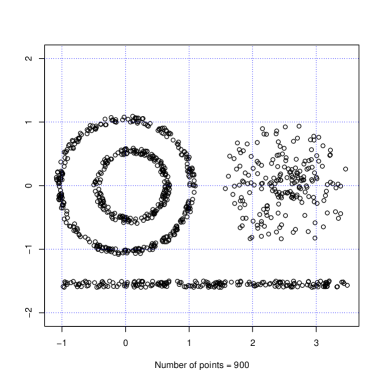
We consider an i.i.d. set {X1,,Xn}2subscript𝑋1subscript𝑋𝑛superscript2\left\{X_{1},\dots,X_{n}\right\}\subset\mathbb{R}^{2} of n=900𝑛900n=900 points to cluster, whose configuration is shown in Figure  1 and we fix the maximum number of classes p=7.𝑝7p=7.
Refer to caption
Figure 1: The data configuration.

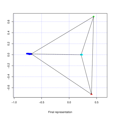
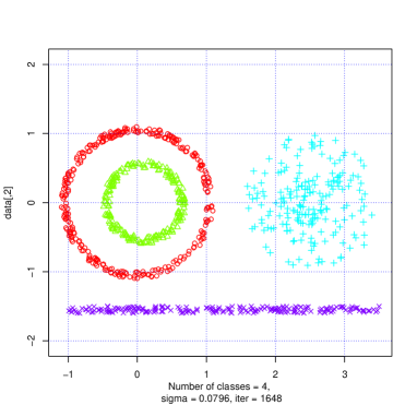
Figure  2 shows that the new representation, induced by the change of kernel, groups the data points at the vertices of the simplex generated by the largest eigenvectors of the matrix C𝐶C, defined in  equation 7. On the left we plot the projection of the simplex along the two first coordinates. This simple configuration allows us to compute the classification, including the number of clusters, using the straightforward greedy algorithm described in Remark 6.
Refer to caption
Refer to caption
Figure 2: On the left the simplex generated by the eigenvectors of C𝐶C, on the right classification performed on C𝐶C.

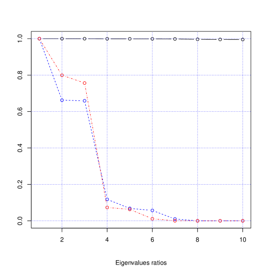
In Figure  3 we plot the first eigenvalues of M𝑀M in black (joined by a solid line), the eigenvalues of its iteration Mmsuperscript𝑀𝑚M^{m} in blue (joined by a dashed line) and the eigenvalues of the covariance matrix of the final representation (defined by C𝐶{C}) in red (joined by a dash-dotted line). We observe that the first eigenvalues of M𝑀M are close to one, while there is a remarkable gap between the eigenvalues of its iteration. In particular the size of the gap is larger once we have renormalized it using the matrix C𝐶C. The number of iterations is automatically estimated and it is equal to 1648.16481648.
Refer to caption
Figure 3: In black (solid line) the eigenvalues of M𝑀M, in blue (dashed line) those of Mmsuperscript𝑀𝑚M^{m} and in red (dash-dot line) the eigenvalues of C𝐶C.

4.2 Some Perspectives on Invariant Shape Analysis

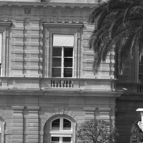
As we have already mentioned in the introduction, we now present a small example about image classification showning how our approach may lead to learn transformation-invariant representations from data sets containing small successive transformations of a same pattern. We briefly describe this approach to get a hint of its potential. We consider two images (Figure  4) and we create our patterns by translating a subwindow of a given size in each image repeatedly, using a translation vector smaller than the subwindow size. In such a way we create a sample consisting of two classes of connected images, as shown in Figure  5. This notion of translation cannot be grasped easily by a mathematical definition, because we do not translate a function but a window of observation. Hence in this case the translation depends on the image content and it may not be easy to model in any realistic situation.
We present, on an example, a successful scenario in which we use first a change of representation in a reproducing kernel Hilbert space to better separate the two classes, and then spectral clustering to shrink each class to a tight blob. This suggests that the so called kernel trick, introduced to better separate classes in the supervised learning framework of support vector machines (SVMs), also works in an unsupervised context. In this setting, we do not separate classes using hyperplanes, since we do not know the class labels which would be necessary to run a SVM, but, instead, we use spectral clustering to finish the work.

Refer to caption
Refer to caption
Figure 4: The two original images.
Refer to caption
Refer to caption
Refer to caption

\cdots Refer to caption Refer to caption \cdots Refer to caption Refer to caption Refer to caption

Refer to caption
Refer to caption
Refer to caption

\cdots Refer to caption Refer to caption \cdots Refer to caption Refer to caption Refer to caption

Figure 5: Our sample consisting of two classes of connected images, the first sequence is obtained with a horizontal translation, the second one with a diagonal translation.

Let X1,,Xnsubscript𝑋1subscript𝑋𝑛X_{1},\dots,X_{n} be the sample of images shown in Figure  5. Each photo is represented as a matrix whose entries are the gray values of the corresponding pixels. We apply twice the change of representation described by the change of kernel in order to better separate clusters. We first consider the reproducing kernel Hilbert space 1subscript1\mathcal{H}_{1} defined by

k1(x,y)=exp(β1xy2)subscript𝑘1𝑥𝑦subscript𝛽1superscriptnorm𝑥𝑦2k_{1}(x,y)=\exp\left(-\beta_{1}\|x-y\|^{2}\right)

and then the reproducing kernel Hilbert space 2subscript2\mathcal{H}_{2} defined by

k2(x,y)=exp(β2xy12)subscript𝑘2𝑥𝑦subscript𝛽2superscriptsubscriptnorm𝑥𝑦subscript12\displaystyle k_{2}(x,y)=\exp\left(-\beta_{2}\|x-y\|_{\mathcal{H}_{1}}^{2}\right) =exp(2β2(1k1(x,y)))absent2subscript𝛽21subscript𝑘1𝑥𝑦\displaystyle=\exp\Bigl{(}-2\beta_{2}\bigl{(}1-k_{1}(x,y)\bigr{)}\Bigr{)}
=exp[2β2(1exp(β1xy2))]absent2subscript𝛽21subscript𝛽1superscriptnorm𝑥𝑦2\displaystyle=\exp\left[-2\beta_{2}\left(1-\exp\left(-\beta_{1}\|x-y\|^{2}\right)\right)\right]

where β1,β2>0subscript𝛽1subscript𝛽20\beta_{1},\beta_{2}>0 are obtained as described in Section 2.3. Define the new kernel

K(x,y)=exp(βxy22),𝐾𝑥𝑦𝛽superscriptsubscriptnorm𝑥𝑦subscript22K(x,y)=\exp\left(-\beta\|x-y\|_{\mathcal{H}_{2}}^{2}\right),

where the parameter β>0𝛽0\beta>0 is chosen again as in Section 2.3, and apply the algorithm described in Section 3.2.

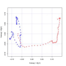
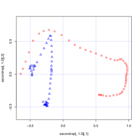
In Figure  6 we compare the representation of the images in the initial space and in the space 2.subscript2\mathcal{H}_{2}. On the left we present the projection of the sample onto the space spanned by the first two largest eigenvectors of the matrix of inner products between images Xi,Xj.subscript𝑋𝑖subscript𝑋𝑗\langle X_{i},X_{j}\rangle. On the right we plot the projection onto the space spanned by the two largest eigenvectors of the matrix of inner products k2(Xi,Xj)subscript𝑘2subscript𝑋𝑖subscript𝑋𝑗k_{2}(X_{i},X_{j}) in 2subscript2\mathcal{H}_{2}. We observe that in the first representation the two classes intersect each other while in the second one, after the change of representation, they are already separated.
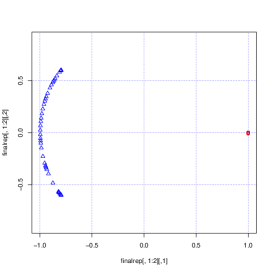
To conclude, Figure  7 shows the final representation. Here the data points are projected onto the space spanned by the two largest eigenvectors of the matrix Mm.superscript𝑀𝑚M^{m}. In this case the number of iteration m𝑚m is of order of 30.00030.00030.000.

Refer to caption
Refer to caption
Figure 6: On the left the projection onto the space spanned by the two largest eigenvectors of Xi,Xjsubscript𝑋𝑖subscript𝑋𝑗\langle X_{i},X_{j}\rangle, on the right the projection onto the space spanned by the two largest eigenvectors of k2(Xi,Xj)subscript𝑘2subscript𝑋𝑖subscript𝑋𝑗k_{2}(X_{i},X_{j}).
Refer to caption
Figure 7: The projection onto the space spanned by the two largest eigenvectors of Mm.superscript𝑀𝑚M^{m}.

5 Proofs

We introduce a technical result that is useful in the following. Let 𝒢𝒢\mathcal{G} be the Gram operator defined in  equation 4 such that 𝒢=1subscriptnorm𝒢1\|\mathcal{G}\|_{\infty}=1 and let 𝒬^^𝒬\widehat{\mathcal{Q}} be its estimator introduced in Section 3.1.

Lemma 13. For any m>0𝑚0m>0

𝒬^m𝒢m\displaystyle\lVert\widehat{\mathcal{Q}}^{m}-\mathcal{G}^{m}\lVert_{\infty} (1+𝒬^𝒢)m1absentsuperscript1subscriptdelimited-∥∥^𝒬𝒢𝑚1\displaystyle\leq\Bigl{(}1+\lVert\widehat{\mathcal{Q}}-\mathcal{G}\rVert_{\infty}\Bigr{)}^{m}-1
m𝒬^𝒢(1+𝒬^𝒢)m1.absent𝑚subscriptdelimited-∥∥^𝒬𝒢superscript1subscriptdelimited-∥∥^𝒬𝒢𝑚1\displaystyle\leq m\lVert\widehat{\mathcal{Q}}-\mathcal{G}\rVert_{\infty}\Bigl{(}1+\lVert\widehat{\mathcal{Q}}-\mathcal{G}\rVert_{\infty}\Bigr{)}^{m-1}.
Proof.

Since

𝒬^m𝒢m=k=0m1𝒬^k(𝒬^𝒢)𝒢mk1,superscript^𝒬𝑚superscript𝒢𝑚superscriptsubscript𝑘0𝑚1superscript^𝒬𝑘^𝒬𝒢superscript𝒢𝑚𝑘1\widehat{\mathcal{Q}}^{m}-\mathcal{G}^{m}=\sum_{k=0}^{m-1}\widehat{\mathcal{Q}}^{k}(\widehat{\mathcal{Q}}-\mathcal{G})\mathcal{G}^{m-k-1},

using the fact that 𝒢=1subscriptnorm𝒢1\|\mathcal{G}\|_{\infty}=1 we get

𝒬^m𝒢m𝒬^𝒢k=0m1𝒬^k.subscriptdelimited-∥∥superscript^𝒬𝑚superscript𝒢𝑚subscriptdelimited-∥∥^𝒬𝒢superscriptsubscript𝑘0𝑚1superscriptsubscriptdelimited-∥∥^𝒬𝑘\lVert\widehat{\mathcal{Q}}^{m}-\mathcal{G}^{m}\rVert_{\infty}\leq\lVert\widehat{\mathcal{Q}}-\mathcal{G}\rVert_{\infty}\sum_{k=0}^{m-1}\lVert\widehat{\mathcal{Q}}\rVert_{\infty}^{k}.

Hence, as 𝒬^1+𝒬^𝒢subscriptdelimited-∥∥^𝒬1subscriptdelimited-∥∥^𝒬𝒢\lVert\widehat{\mathcal{Q}}\rVert_{\infty}\leq 1+\lVert\widehat{\mathcal{Q}}-\mathcal{G}\rVert_{\infty}, we conclude

𝒬^m𝒢m(1+𝒬^𝒢)m1=𝒬^𝒢k=0m1(1+𝒬^𝒢)km𝒬^𝒢(1+𝒬^𝒢)m1.subscriptdelimited-∥∥superscript^𝒬𝑚superscript𝒢𝑚superscript1subscriptdelimited-∥∥^𝒬𝒢𝑚1subscriptdelimited-∥∥^𝒬𝒢superscriptsubscript𝑘0𝑚1superscript1subscriptdelimited-∥∥^𝒬𝒢𝑘𝑚subscriptdelimited-∥∥^𝒬𝒢superscript1subscriptdelimited-∥∥^𝒬𝒢𝑚1\lVert\widehat{\mathcal{Q}}^{m}-\mathcal{G}^{m}\rVert_{\infty}\leq\Bigl{(}1+\lVert\widehat{\mathcal{Q}}-\mathcal{G}\rVert_{\infty}\Bigr{)}^{m}-1\\ =\lVert\widehat{\mathcal{Q}}-\mathcal{G}\rVert_{\infty}\sum_{k=0}^{m-1}\bigl{(}1+\lVert\widehat{\mathcal{Q}}-\mathcal{G}\rVert_{\infty}\bigr{)}^{k}\leq m\lVert\widehat{\mathcal{Q}}-\mathcal{G}\rVert_{\infty}\bigl{(}1+\lVert\widehat{\mathcal{Q}}-\mathcal{G}\rVert_{\infty}\bigr{)}^{m-1}.

\blacksquare

We also introduce the intermediate operator 𝒢~::~𝒢\widetilde{\mathcal{G}}:\mathcal{H}\to\mathcal{H}

𝒢~u=u,ϕK^(z)ϕK^(z)dP(z)~𝒢𝑢subscript𝑢subscriptitalic-ϕ^𝐾𝑧subscriptitalic-ϕ^𝐾𝑧dP𝑧\widetilde{\mathcal{G}}u=\int\left\langle u,\phi_{\widehat{K}}(z)\right\rangle_{\mathcal{H}}\ \phi_{\widehat{K}}(z)\,\mathrm{d}\mathrm{P}(z)

where, according to the notation of Section 3, ϕK^(x)=χ(x)ϕK¯(x)subscriptitalic-ϕ^𝐾𝑥𝜒𝑥subscriptitalic-ϕ¯𝐾𝑥\phi_{\widehat{K}}(x)=\chi(x)\phi_{\overline{K}}(x) and χ(x)=(μ(x)/μ^(x))1/2.𝜒𝑥superscript𝜇𝑥^𝜇𝑥12\chi(x)=\big{(}\mu(x)/\widehat{\mu}(x)\big{)}^{1/2}.

5.1 Proof of Proposition 8

To prove the first inequality, we define

(x,y)=|K^2m(x,y)K¯2m(x,y)|𝑥𝑦subscript^𝐾2𝑚𝑥𝑦subscript¯𝐾2𝑚𝑥𝑦\mathcal{E}(x,y)=\bigl{\lvert}\widehat{K}_{2m}(x,y)-\overline{K}_{2m}(x,y)\bigr{\rvert}

and we observe that, according to Lemma 13, it is sufficient to show that

(x,y)max{1,χ}2μ(x)1/2μ(y)1/2(𝒬^2m1𝒢2m1+2χ1).\mathcal{E}(x,y)\leq\frac{\displaystyle\max\{1,\lVert\chi\rVert_{\infty}\}^{2}}{\mu(x)^{1/2}\mu(y)^{1/2}}\Bigl{(}\lVert\widehat{\mathcal{Q}}^{2m-1}-\mathcal{G}^{2m-1}\rVert_{\infty}+2\lVert\chi-1\rVert_{\infty}\Bigr{)}. (9)

By definition,

(x,y)=|𝒬^2m1ϕK^(x),ϕK^(y)𝒢2m1ϕK¯(x),ϕK¯(y)||(𝒬^2m1𝒢2m1)ϕK^(x),ϕK^(y)|+|𝒢2m1(ϕK^(x)ϕK¯(x)),ϕK^(y)|+𝒢2m1ϕK¯(x),(ϕK^(y)ϕK¯(y))|.\mathcal{E}(x,y)=\bigl{\lvert}\left\langle\widehat{\mathcal{Q}}^{2m-1}\phi_{\widehat{K}}(x),\phi_{\widehat{K}}(y)\right\rangle_{\mathcal{H}}-\left\langle\mathcal{G}^{2m-1}\phi_{\overline{K}}(x),\phi_{\overline{K}}(y)\right\rangle_{\mathcal{H}}\bigr{\rvert}\\ \leq\bigl{\lvert}\left\langle(\widehat{\mathcal{Q}}^{2m-1}-\mathcal{G}^{2m-1})\phi_{\widehat{K}}(x),\phi_{\widehat{K}}(y)\right\rangle_{\mathcal{H}}\bigr{\rvert}+\bigl{\lvert}\left\langle\mathcal{G}^{2m-1}\bigl{(}\phi_{\widehat{K}}(x)-\phi_{\overline{K}}(x)\bigr{)},\phi_{\widehat{K}}(y)\right\rangle_{\mathcal{H}}\bigr{\rvert}\\ +\left\langle\mathcal{G}^{2m-1}\phi_{\overline{K}}(x),\bigl{(}\phi_{\widehat{K}}(y)-\phi_{\overline{K}}(y)\bigr{)}\right\rangle_{\mathcal{H}}\bigr{\rvert}.

Recalling the definition of ϕK^,subscriptitalic-ϕ^𝐾\phi_{\widehat{K}}, we get

(x,y)𝒬^2m1𝒢2m1χ2ϕK¯(x)ϕK¯(y)+χ1(χ+1)ϕK¯(x)ϕK¯(y),𝑥𝑦subscriptdelimited-∥∥superscript^𝒬2𝑚1superscript𝒢2𝑚1superscriptsubscriptdelimited-∥∥𝜒2subscriptdelimited-∥∥subscriptitalic-ϕ¯𝐾𝑥subscriptdelimited-∥∥subscriptitalic-ϕ¯𝐾𝑦subscriptdelimited-∥∥𝜒1subscriptdelimited-∥∥𝜒1subscriptdelimited-∥∥subscriptitalic-ϕ¯𝐾𝑥subscriptdelimited-∥∥subscriptitalic-ϕ¯𝐾𝑦\mathcal{E}(x,y)\leq\lVert\widehat{\mathcal{Q}}^{2m-1}-\mathcal{G}^{2m-1}\rVert_{\infty}\lVert\chi\rVert_{\infty}^{2}\lVert\phi_{\overline{K}}(x)\rVert_{\mathcal{H}}\lVert\phi_{\overline{K}}(y)\rVert_{\mathcal{H}}+\lVert\chi-1\rVert_{\infty}\bigl{(}\lVert\chi\rVert_{\infty}+1\bigr{)}\lVert\phi_{\overline{K}}(x)\rVert_{\mathcal{H}}\lVert\phi_{\overline{K}}(y)\rVert_{\mathcal{H}},

where, since K(x,x)=1𝐾𝑥𝑥1K(x,x)=1,

ϕK¯(x)2=K¯(x,x)=K(x,x)μ(x)1/2μ(x)1/2=1μ(x).superscriptsubscriptdelimited-∥∥subscriptitalic-ϕ¯𝐾𝑥2¯𝐾𝑥𝑥𝐾𝑥𝑥𝜇superscript𝑥12𝜇superscript𝑥121𝜇𝑥\lVert\phi_{\overline{K}}(x)\rVert_{\mathcal{H}}^{2}=\overline{K}(x,x)=\frac{K(x,x)}{\mu(x)^{1/2}\mu(x)^{1/2}}=\frac{1}{\mu(x)}.

This proves  equation 9. To prove the second bound we define

(x)=((x,y)2dP(y))1/2𝑥superscriptsuperscript𝑥𝑦2dP𝑦12\mathcal{E}(x)=\Biggl{(}\int\mathcal{E}(x,y)^{2}\,\mathrm{d}\mathrm{P}(y)\Biggr{)}^{1/2}

so that using Lemma 13 again, it is sufficient to show that

(x)max{1,χ}2μ(x)1/2(𝒬^2m1𝒢2m1+2χ1).\mathcal{E}(x)\leq\frac{\displaystyle\max\{1,\lVert\chi\rVert_{\infty}\}^{2}}{\mu(x)^{1/2}}\Bigl{(}\lVert\widehat{\mathcal{Q}}^{2m-1}-\mathcal{G}^{2m-1}\rVert_{\infty}+2\lVert\chi-1\rVert_{\infty}\Bigr{)}.

Observe that

(x)=((𝒬^2m1ϕK^(x),ϕK^(y)𝒢2m1ϕK¯(x),ϕK¯(y))2dP(y))1/2((𝒬^2m1𝒢2m1)ϕK^(x),ϕK^(y)2dP(y))1/2+(𝒢2m1(ϕK^(x)ϕK¯(x)),ϕK^(y)2dP(y))1/2+(𝒢2m1ϕK¯(x),ϕK^(y)ϕK¯(y)2dP(y))1/2.formulae-sequence𝑥superscriptsuperscriptsubscriptsuperscript^𝒬2𝑚1subscriptitalic-ϕ^𝐾𝑥subscriptitalic-ϕ^𝐾𝑦subscriptsuperscript𝒢2𝑚1subscriptitalic-ϕ¯𝐾𝑥subscriptitalic-ϕ¯𝐾𝑦2dP𝑦12superscriptsuperscriptsubscriptsuperscript^𝒬2𝑚1superscript𝒢2𝑚1subscriptitalic-ϕ^𝐾𝑥subscriptitalic-ϕ^𝐾𝑦2dP𝑦12superscriptsuperscriptsubscriptsuperscript𝒢2𝑚1subscriptitalic-ϕ^𝐾𝑥subscriptitalic-ϕ¯𝐾𝑥subscriptitalic-ϕ^𝐾𝑦2dP𝑦12superscriptsuperscriptsubscriptsuperscript𝒢2𝑚1subscriptitalic-ϕ¯𝐾𝑥subscriptitalic-ϕ^𝐾𝑦subscriptitalic-ϕ¯𝐾𝑦2dP𝑦12\mathcal{E}(x)=\Biggl{(}\int\Bigl{(}\left\langle\widehat{\mathcal{Q}}^{2m-1}\phi_{\widehat{K}}(x),\phi_{\widehat{K}}(y)\right\rangle_{\mathcal{H}}-\left\langle\mathcal{G}^{2m-1}\phi_{\overline{K}}(x),\phi_{\overline{K}}(y)\right\rangle_{\mathcal{H}}\Bigr{)}^{2}\,\mathrm{d}\mathrm{P}(y)\Biggr{)}^{1/2}\\ \leq\Biggl{(}\int\left\langle\bigl{(}\widehat{\mathcal{Q}}^{2m-1}-\mathcal{G}^{2m-1}\bigr{)}\phi_{\widehat{K}}(x),\phi_{\widehat{K}}(y)\right\rangle_{\mathcal{H}}^{2}\,\mathrm{d}\mathrm{P}(y)\Biggr{)}^{1/2}\\ \qquad\qquad\qquad+\Biggl{(}\int\bigl{\langle}\mathcal{G}^{2m-1}\bigl{(}\phi_{\widehat{K}}(x)-\phi_{\overline{K}}(x)\bigr{)},\phi_{\widehat{K}}(y)\bigr{\rangle}_{\mathcal{H}}^{2}\,\mathrm{d}\mathrm{P}(y)\Biggr{)}^{1/2}\\ +\Biggl{(}\int\left\langle\mathcal{G}^{2m-1}\phi_{\overline{K}}(x),\phi_{\widehat{K}}(y)-\phi_{\overline{K}}(y)\right\rangle_{\mathcal{H}}^{2}\,\mathrm{d}\mathrm{P}(y)\Biggr{)}^{1/2}.

By definition of 𝒢~~𝒢\widetilde{\mathcal{G}} we get

(x)𝒢~1/2(𝒬^2m1𝒢2m1)ϕK^(x)+𝒢~1/2𝒢2m1(ϕK^(x)ϕ(x))+χ1𝒢2m1/2ϕ(x).𝑥subscriptdelimited-∥∥superscript~𝒢12superscript^𝒬2𝑚1superscript𝒢2𝑚1subscriptitalic-ϕ^𝐾𝑥subscriptdelimited-∥∥superscript~𝒢12superscript𝒢2𝑚1subscriptitalic-ϕ^𝐾𝑥italic-ϕ𝑥subscriptdelimited-∥∥𝜒1subscriptdelimited-∥∥superscript𝒢2𝑚12italic-ϕ𝑥\mathcal{E}(x)\leq\bigl{\lVert}\widetilde{\mathcal{G}}^{1/2}\bigl{(}\widehat{\mathcal{Q}}^{2m-1}-\mathcal{G}^{2m-1}\bigr{)}\phi_{\widehat{K}}(x)\bigr{\rVert}_{\mathcal{H}}+\bigl{\lVert}\widetilde{\mathcal{G}}^{1/2}\mathcal{G}^{2m-1}\bigl{(}\phi_{\widehat{K}}(x)-\phi(x)\bigr{)}\rVert_{\mathcal{H}}\\ +\lVert\chi-1\rVert_{\infty}\bigl{\lVert}\mathcal{G}^{2m-1/2}\phi(x)\bigr{\rVert}_{\mathcal{H}}.

Thus using the fact that 𝒢=1subscriptnorm𝒢1\|\mathcal{G}\|_{\infty}=1 and that, for any u𝑢u\in\mathcal{H},

𝒢~1/2u2=𝒢~u,u=u,ϕK^(y)2dP(y)χ2𝒢u,u,superscriptsubscriptnormsuperscript~𝒢12𝑢2subscript~𝒢𝑢𝑢superscriptsubscript𝑢subscriptitalic-ϕ^𝐾𝑦2dP𝑦superscriptsubscriptdelimited-∥∥𝜒2𝒢𝑢𝑢\|\widetilde{\mathcal{G}}^{1/2}u\|_{\mathcal{H}}^{2}=\langle\widetilde{\mathcal{G}}u,u\rangle_{\mathcal{H}}=\int\langle u,\phi_{\widehat{K}}(y)\rangle_{\mathcal{H}}^{2}\ \mathrm{d}\mathrm{P}(y)\leq\lVert\chi\rVert_{\infty}^{2}\langle\mathcal{G}u,u\rangle,

we conclude.

5.2 Proof of Proposition 9

In order to prove the two inequalities we need to introduce some preliminary results. Consider the operator 𝒮:LP2:𝒮superscriptsubscript𝐿P2\mathcal{S}:\mathcal{H}\to L_{\mathrm{P}}^{2}

𝒮(u):xu,ϕK¯(x).:𝒮𝑢maps-to𝑥subscript𝑢subscriptitalic-ϕ¯𝐾𝑥\mathcal{S}(u):x\mapsto\langle u,\phi_{\overline{K}}(x)\rangle_{\mathcal{H}}.

Introduce the operator 𝐆:LP2LP2:𝐆superscriptsubscript𝐿P2superscriptsubscript𝐿P2\mathbf{G}:L_{\mathrm{P}}^{2}\to L_{\mathrm{P}}^{2}

𝐆(f)(x)=𝒮𝒮f(x)=K¯(x,y)f(y)dP(y)𝐆𝑓𝑥𝒮superscript𝒮𝑓𝑥¯𝐾𝑥𝑦𝑓𝑦dP𝑦\mathbf{G}(f)(x)=\mathcal{S}\mathcal{S}^{*}f(x)=\int\overline{K}(x,y)f(y)\,\mathrm{d}\mathrm{P}(y)

and observe that the Gram operator 𝒢𝒢\mathcal{G} rewrites as

𝒢u=𝒮𝒮u=u,ϕK¯(z)ϕK¯(z)dP(z).𝒢𝑢superscript𝒮𝒮𝑢subscript𝑢subscriptitalic-ϕ¯𝐾𝑧subscriptitalic-ϕ¯𝐾𝑧dP𝑧\mathcal{G}u=\mathcal{S}^{*}\mathcal{S}u=\int\langle u,\phi_{\overline{K}}(z)\rangle_{\mathcal{H}}\ \phi_{\overline{K}}(z)\ \mathrm{d}\mathrm{P}(z).

Moreover 𝐆=𝒢=1.subscriptnorm𝐆subscriptnorm𝒢1\|\mathbf{G}\|_{\infty}=\|\mathcal{G}\|_{\infty}=1.

Lemma 14. We have

𝐈𝐦(𝐆)=𝒮(𝐈𝐦(𝒢))=𝒮(𝐈𝐦(𝒢~)).𝐈𝐦𝐆𝒮𝐈𝐦𝒢𝒮𝐈𝐦~𝒢\operatorname{\mathbf{Im}}(\mathbf{G})=\mathcal{S}\bigl{(}\operatorname{\mathbf{Im}}(\mathcal{G})\bigr{)}=\mathcal{S}\bigl{(}\operatorname{\mathbf{Im}}(\widetilde{\mathcal{G}})\bigr{)}.
Proof.

We observe that, since 𝐆𝐆\mathbf{G} is symmetric, 𝐈𝐦(𝐆)=𝐈𝐦(𝐆2)𝐈𝐦𝐆𝐈𝐦superscript𝐆2\operatorname{\mathbf{Im}}(\mathbf{G})=\operatorname{\mathbf{Im}}(\mathbf{G}^{2}), where 𝐆2=𝒮𝒢𝒮superscript𝐆2𝒮𝒢superscript𝒮\mathbf{G}^{2}=\mathcal{S}\mathcal{G}\mathcal{S}^{*}. Thus 𝐈𝐦(𝐆)=𝐈𝐦(𝐆2)𝒮(𝐈𝐦(𝒢))𝐈𝐦𝐆𝐈𝐦superscript𝐆2𝒮𝐈𝐦𝒢\operatorname{\mathbf{Im}}(\mathbf{G})=\operatorname{\mathbf{Im}}(\mathbf{G}^{2})\subset\mathcal{S}\bigl{(}\operatorname{\mathbf{Im}}(\mathcal{G})\bigr{)}. Since 𝒮𝒢=𝐆𝒮𝒮𝒢𝐆𝒮\mathcal{S}\mathcal{G}=\mathbf{G}\mathcal{S}, we conclude that 𝒮(𝐈𝐦(𝒢))𝐈𝐦𝐆𝒮𝐈𝐦𝒢𝐈𝐦𝐆\mathcal{S}\bigl{(}\operatorname{\mathbf{Im}}(\mathcal{G})\bigr{)}\subset\operatorname{\mathbf{Im}}\mathbf{G}.
To prove the second identity, we remark that, since χ(x)>0𝜒𝑥0\chi(x)>0,

𝐤𝐞𝐫(𝒢~)𝐤𝐞𝐫~𝒢\displaystyle\operatorname{\mathbf{ker}}(\widetilde{\mathcal{G}}) ={u,u,ϕK^(x)2dP(x)=0}absentformulae-sequence𝑢superscript𝑢subscriptitalic-ϕ^𝐾𝑥2dP𝑥0\displaystyle=\biggl{\{}u\in\mathcal{H},\int\langle u,\phi_{\widehat{K}}(x)\rangle^{2}\,\mathrm{d}\mathrm{P}(x)=0\biggr{\}}
={u,u,ϕ(x)2dP(x)=0}=𝐤𝐞𝐫(𝒢).absentformulae-sequence𝑢superscript𝑢italic-ϕ𝑥2dP𝑥0𝐤𝐞𝐫𝒢\displaystyle=\biggl{\{}u\in\mathcal{H},\int\langle u,\phi(x)\rangle^{2}\,\mathrm{d}\mathrm{P}(x)=0\biggr{\}}=\operatorname{\mathbf{ker}}(\mathcal{G}).

Consequently, since 𝐈𝐦(𝒢)=𝐤𝐞𝐫(𝒢)\operatorname{\mathbf{Im}}(\mathcal{G})=\operatorname{\mathbf{ker}}(\mathcal{G})^{\perp}, we get

𝐬𝐩𝐚𝐧¯(ϕ(supp(P)))¯𝐬𝐩𝐚𝐧italic-ϕsupp𝑃\displaystyle\operatorname{\overline{\mathbf{span}}}\Bigl{(}\phi\bigl{(}\operatorname{\mathrm{supp}}(P)\bigr{)}\Bigr{)} =𝐤𝐞𝐫(𝒢)=𝐈𝐦(𝒢)=𝐈𝐦(𝒢~)=𝐬𝐩𝐚𝐧¯(ϕK^(supp(P))).\displaystyle=\operatorname{\mathbf{ker}}(\mathcal{G})^{\perp}=\operatorname{\mathbf{Im}}(\mathcal{G})=\operatorname{\mathbf{Im}}(\widetilde{\mathcal{G}})=\operatorname{\overline{\mathbf{span}}}\Bigl{(}\phi_{\widehat{K}}\bigl{(}\operatorname{\mathrm{supp}}(P)\bigr{)}\Bigr{)}.

\blacksquare

Therefore any f𝐈𝐦(𝐆)𝑓𝐈𝐦𝐆f\in\operatorname{\mathbf{Im}}(\mathbf{G}) is of the form f=𝒮u𝑓𝒮𝑢f=\mathcal{S}u, with u𝐈𝐦(𝒢),𝑢𝐈𝐦𝒢u\in\operatorname{\mathbf{Im}}(\mathcal{G}), so that we can estimate

fLP22=𝒢u,usuperscriptsubscriptdelimited-∥∥𝑓superscriptsubscript𝐿P22subscript𝒢𝑢𝑢\lVert f\rVert_{L_{\mathrm{P}}^{2}}^{2}=\langle\mathcal{G}u,u\rangle_{\mathcal{H}}

by 𝒬^u,usubscript^𝒬𝑢𝑢\langle\widehat{\mathcal{Q}}u,u\rangle_{\mathcal{H}}. The estimation error is bounded as described in the following lemma.

Lemma 15. For any u,v𝑢𝑣u,v\in\mathcal{H},

|𝒮u,𝒮vLP2𝒬^u,v|𝒢𝒬^uv.subscript𝒮𝑢𝒮𝑣superscriptsubscript𝐿P2subscript^𝒬𝑢𝑣subscriptdelimited-∥∥𝒢^𝒬subscriptdelimited-∥∥𝑢subscriptdelimited-∥∥𝑣\bigl{\lvert}\langle\mathcal{S}u,\mathcal{S}v\rangle_{L_{\mathrm{P}}^{2}}-\langle\widehat{\mathcal{Q}}u,v\rangle_{\mathcal{H}}\bigr{\rvert}\leq\lVert\mathcal{G}-\widehat{\mathcal{Q}}\rVert_{\infty}\lVert u\rVert_{\mathcal{H}}\lVert v\rVert_{\mathcal{H}}.

In particular,

|𝒮uLP22𝒬^u,u|𝒢𝒬^u2.subscriptsuperscriptdelimited-∥∥𝒮𝑢2superscriptsubscript𝐿P2subscript^𝒬𝑢𝑢subscriptdelimited-∥∥𝒢^𝒬subscriptsuperscriptdelimited-∥∥𝑢2\bigl{\lvert}\lVert\mathcal{S}u\rVert^{2}_{L_{\mathrm{P}}^{2}}-\langle\widehat{\mathcal{Q}}u,u\rangle_{\mathcal{H}}\bigr{\rvert}\leq\lVert\mathcal{G}-\widehat{\mathcal{Q}}\rVert_{\infty}\lVert u\rVert^{2}_{\mathcal{H}}.
Proof.

It is sufficient to observe that 𝒮u,𝒮vLP2=𝒢u,vsubscript𝒮𝑢𝒮𝑣superscriptsubscript𝐿P2subscript𝒢𝑢𝑣\langle\mathcal{S}u,\mathcal{S}v\rangle_{L_{\mathrm{P}}^{2}}=\langle\mathcal{G}u,v\rangle_{\mathcal{H}}. \blacksquare

We now observe that

𝐑xsubscript𝐑𝑥\displaystyle\mathbf{R}_{x} =𝒮𝒢m1ϕK¯(x)𝐈𝐦(𝐆)absent𝒮superscript𝒢𝑚1subscriptitalic-ϕ¯𝐾𝑥𝐈𝐦𝐆\displaystyle=\mathcal{S}\mathcal{G}^{m-1}{\phi_{\overline{K}}}(x)\in\operatorname{\mathbf{Im}}(\mathbf{G}) (10)
𝐑^xsubscript^𝐑𝑥\displaystyle\widehat{\mathbf{R}}_{x} =𝒮𝒬^m1ϕK^(x)𝐈𝐦(𝐆)almost surely.formulae-sequenceabsent𝒮superscript^𝒬𝑚1subscriptitalic-ϕ^𝐾𝑥𝐈𝐦𝐆almost surely\displaystyle=\mathcal{S}\widehat{\mathcal{Q}}^{m-1}\phi_{\widehat{K}}(x)\in\operatorname{\mathbf{Im}}(\mathbf{G})\quad\text{almost surely}.

Indeed, by definition,

𝐑^x=𝒮𝒬^m1ϕK^(x)and𝐑x=𝒮𝒢m1ϕK¯(x).formulae-sequencesubscript^𝐑𝑥𝒮superscript^𝒬𝑚1subscriptitalic-ϕ^𝐾𝑥andsubscript𝐑𝑥𝒮superscript𝒢𝑚1subscriptitalic-ϕ¯𝐾𝑥\displaystyle\widehat{\mathbf{R}}_{x}=\mathcal{S}\widehat{\mathcal{Q}}^{m-1}\phi_{\widehat{K}}(x)\quad\text{and}\quad\mathbf{R}_{x}=\mathcal{S}\mathcal{G}^{m-1}{\phi}_{\overline{K}}(x).

Hence, since

𝐈𝐦(𝐆)=𝒮(𝐈𝐦(𝒢))=𝒮(𝐬𝐩𝐚𝐧¯ϕK¯(supp(P))),𝐈𝐦𝐆𝒮𝐈𝐦𝒢𝒮¯𝐬𝐩𝐚𝐧subscriptitalic-ϕ¯𝐾suppP\operatorname{\mathbf{Im}}(\mathbf{G})=\mathcal{S}\bigl{(}\operatorname{\mathbf{Im}}(\mathcal{G})\bigr{)}=\mathcal{S}\Bigl{(}\operatorname{\overline{\mathbf{span}}}\phi_{\overline{K}}\bigl{(}\operatorname{\mathrm{supp}}(\mathrm{P})\bigr{)}\Bigr{)},

we conclude that 𝐑x𝐈𝐦(𝐆)subscript𝐑𝑥𝐈𝐦𝐆\mathbf{R}_{x}\in\operatorname{\mathbf{Im}}(\mathbf{G}). Moreover, since

𝐬𝐩𝐚𝐧{ϕK^(Xn),,ϕK^(X2n)}𝐬𝐩𝐚𝐧subscriptitalic-ϕ^𝐾subscript𝑋𝑛subscriptitalic-ϕ^𝐾subscript𝑋2𝑛\displaystyle\operatorname{\mathbf{span}}\bigl{\{}\phi_{\widehat{K}}(X_{n}),\dots,\phi_{\widehat{K}}(X_{2n})\bigr{\}} =𝐬𝐩𝐚𝐧{ϕK¯(Xn),,ϕK¯(X2n)}absent𝐬𝐩𝐚𝐧subscriptitalic-ϕ¯𝐾subscript𝑋𝑛subscriptitalic-ϕ¯𝐾subscript𝑋2𝑛\displaystyle=\operatorname{\mathbf{span}}\bigl{\{}\phi_{\overline{K}}(X_{n}),\dots,\phi_{\overline{K}}(X_{2n})\bigr{\}}
𝐬𝐩𝐚𝐧¯(ϕK¯(supp(P)))almost surely,absent¯𝐬𝐩𝐚𝐧subscriptitalic-ϕ¯𝐾suppPalmost surely,\displaystyle\subset\operatorname{\overline{\mathbf{span}}}\Bigl{(}\phi_{\overline{K}}\bigl{(}\operatorname{\mathrm{supp}}(\mathrm{P})\bigr{)}\Bigr{)}\quad\text{almost surely,}

it is also true that 𝐑^x𝐈𝐦(𝐆)subscript^𝐑𝑥𝐈𝐦𝐆\widehat{\mathbf{R}}_{x}\in\operatorname{\mathbf{Im}}(\mathbf{G}).

We can now prove the two bounds presented in the proposition. Define

r(x)subscript𝑟𝑥\displaystyle\mathcal{E}_{r}(x) =𝐑x𝐑^xLP2absentsubscriptdelimited-∥∥subscript𝐑𝑥subscript^𝐑𝑥superscriptsubscript𝐿P2\displaystyle=\bigl{\lVert}\mathbf{R}_{x}-\widehat{\mathbf{R}}_{x}\bigr{\rVert}_{L_{\mathrm{P}}^{2}}
c(f)subscript𝑐𝑓\displaystyle\mathcal{E}_{c}(f) =(𝐑x𝐑^x,fLP22dP(x))1/2.absentsuperscriptsubscriptsuperscriptsubscript𝐑𝑥subscript^𝐑𝑥𝑓2superscriptsubscript𝐿P2dP𝑥12\displaystyle=\Biggl{(}\int\Bigl{\langle}\mathbf{R}_{x}-\widehat{\mathbf{R}}_{x},f\Bigr{\rangle}^{2}_{L_{\mathrm{P}}^{2}}\,\mathrm{d}\mathrm{P}(x)\Biggr{)}^{1/2}.

According to Lemma 13, it is sufficient to show that, for any xsupp(P)𝑥suppPx\in\operatorname{\mathrm{supp}}(\mathrm{P}), fLP2,𝑓subscriptsuperscript𝐿2Pf\in{L}^{2}_{\mathrm{P}},

r(x)subscript𝑟𝑥\displaystyle\mathcal{E}_{r}(x) μ(x)1/2(χ𝒬^m1𝒢m1+χ1)absent𝜇superscript𝑥12subscriptdelimited-∥∥𝜒subscriptdelimited-∥∥superscript^𝒬𝑚1superscript𝒢𝑚1subscriptdelimited-∥∥𝜒1\displaystyle\leq\mu(x)^{-1/2}\Bigl{(}\lVert\chi\rVert_{\infty}\lVert\widehat{\mathcal{Q}}^{m-1}-\mathcal{G}^{m-1}\rVert_{\infty}+\lVert\chi-1\rVert_{\infty}\Bigr{)}
c(f)subscript𝑐𝑓\displaystyle\mathcal{E}_{c}(f) fLP2(χ𝒬^m1𝒢m1+χ1).\displaystyle\leq\lVert f\rVert_{L_{\mathrm{P}}^{2}}\Bigl{(}\lVert\chi\rVert_{\infty}\lVert\widehat{\mathcal{Q}}^{m-1}-\mathcal{G}^{m-1}\lVert_{\infty}+\lVert\chi-1\rVert_{\infty}\Bigr{)}.

In order to prove the first inequality, we observe that

r(x)subscript𝑟𝑥\displaystyle\mathcal{E}_{r}(x) =𝒮𝒬^m1ϕK^(x)𝒮𝒢m1ϕK¯(x)LP2absentsubscriptdelimited-∥∥𝒮superscript^𝒬𝑚1subscriptitalic-ϕ^𝐾𝑥𝒮superscript𝒢𝑚1subscriptitalic-ϕ¯𝐾𝑥superscriptsubscript𝐿P2\displaystyle=\bigl{\lVert}\mathcal{S}\widehat{\mathcal{Q}}^{m-1}\phi_{\widehat{K}}(x)-\mathcal{S}\mathcal{G}^{m-1}\phi_{\overline{K}}(x)\bigr{\rVert}_{L_{\mathrm{P}}^{2}}
𝒮(𝒬^m1𝒢m1)ϕK^(x)LP2+𝒮𝒢m1(ϕK^(x)ϕK¯(x))LP2.absentsubscriptdelimited-∥∥𝒮superscript^𝒬𝑚1superscript𝒢𝑚1subscriptitalic-ϕ^𝐾𝑥superscriptsubscript𝐿P2subscriptdelimited-∥∥𝒮superscript𝒢𝑚1subscriptitalic-ϕ^𝐾𝑥subscriptitalic-ϕ¯𝐾𝑥superscriptsubscript𝐿P2\displaystyle\leq\bigl{\lVert}\mathcal{S}\bigl{(}\widehat{\mathcal{Q}}^{m-1}-\mathcal{G}^{m-1}\bigr{)}\phi_{\widehat{K}}(x)\bigr{\rVert}_{L_{\mathrm{P}}^{2}}+\bigl{\lVert}\mathcal{S}\mathcal{G}^{m-1}\bigl{(}\phi_{\widehat{K}}(x)-\phi_{\overline{K}}(x)\bigr{)}\bigr{\rVert}_{L_{\mathrm{P}}^{2}}.

Since 𝒮uLP22=𝒮𝒮u,u=𝒢u,usubscriptsuperscriptdelimited-∥∥𝒮𝑢2superscriptsubscript𝐿P2subscriptsuperscript𝒮𝒮𝑢𝑢subscript𝒢𝑢𝑢\lVert\mathcal{S}u\rVert^{2}_{L_{\mathrm{P}}^{2}}=\langle\mathcal{S}^{*}\mathcal{S}u,u\rangle_{\mathcal{H}}=\langle\mathcal{G}u,u\rangle_{\mathcal{H}}, then 𝒮=𝒢1/2=1subscriptdelimited-∥∥𝒮subscriptsuperscriptdelimited-∥∥𝒢121\lVert\mathcal{S}\rVert_{\infty}=\lVert\mathcal{G}\rVert^{1/2}_{\infty}=1 and hence, recalling the definition of ϕK^,subscriptitalic-ϕ^𝐾\phi_{\widehat{K}}, we get

r(x)𝒬^m1𝒢m1χϕK¯(x)+χ1ϕK¯(x).subscript𝑟𝑥subscriptdelimited-∥∥superscript^𝒬𝑚1superscript𝒢𝑚1subscriptdelimited-∥∥𝜒subscriptdelimited-∥∥subscriptitalic-ϕ¯𝐾𝑥subscriptdelimited-∥∥𝜒1subscriptdelimited-∥∥subscriptitalic-ϕ¯𝐾𝑥\mathcal{E}_{r}(x)\leq\lVert\widehat{\mathcal{Q}}^{m-1}-\mathcal{G}^{m-1}\rVert_{\infty}\lVert\chi\rVert_{\infty}\lVert\phi_{\overline{K}}(x)\rVert_{\mathcal{H}}+\lVert\chi-1\rVert_{\infty}\lVert\phi_{\overline{K}}(x)\rVert_{\mathcal{H}}.

We now prove the second bound. Let 𝚷:LP2LP2:𝚷superscriptsubscript𝐿P2superscriptsubscript𝐿P2\mathbf{\Pi}:L_{\mathrm{P}}^{2}\to L_{\mathrm{P}}^{2} be the orthogonal projector on 𝐈𝐦(𝐆)𝐈𝐦𝐆\operatorname{\mathbf{Im}}(\mathbf{G}). Since, according to  equation 10, almost surely, 𝐑^x𝐑x𝐈𝐦(𝐆)subscript^𝐑𝑥subscript𝐑𝑥𝐈𝐦𝐆\widehat{\mathbf{R}}_{x}-\mathbf{R}_{x}\in\operatorname{\mathbf{Im}}(\mathbf{G}), for any x𝒳𝑥𝒳x\in\mathcal{X}, then

𝐑^x𝐑x,fLP2=𝐑^x𝐑x,𝚷(f)LP2 almost surely.subscriptsubscript^𝐑𝑥subscript𝐑𝑥𝑓superscriptsubscript𝐿P2subscriptsubscript^𝐑𝑥subscript𝐑𝑥𝚷𝑓superscriptsubscript𝐿P2 almost surely.\Bigl{\langle}\widehat{\mathbf{R}}_{x}-\mathbf{R}_{x},f\Bigr{\rangle}_{L_{\mathrm{P}}^{2}}=\Bigl{\langle}\widehat{\mathbf{R}}_{x}-\mathbf{R}_{x},\mathbf{\Pi}(f)\Bigr{\rangle}_{L_{\mathrm{P}}^{2}}\quad\text{ almost surely.}

Moreover, since 𝐈𝐦(𝐆)=𝒮(𝐈𝐦(𝒢))𝐈𝐦𝐆𝒮𝐈𝐦𝒢\operatorname{\mathbf{Im}}(\mathbf{G})=\mathcal{S}\bigl{(}\operatorname{\mathbf{Im}}(\mathcal{G})\bigr{)}, there is u𝐈𝐦(𝒢)𝑢𝐈𝐦𝒢u\in\operatorname{\mathbf{Im}}(\mathcal{G}) such that 𝚷(f)=𝒮u𝚷𝑓𝒮𝑢\mathbf{\Pi}(f)=\mathcal{S}u. We can then write

𝐑^x𝐑x,fLP2subscriptsubscript^𝐑𝑥subscript𝐑𝑥𝑓superscriptsubscript𝐿P2\displaystyle\Bigl{\langle}\widehat{\mathbf{R}}_{x}-\mathbf{R}_{x},f\Bigr{\rangle}_{L_{\mathrm{P}}^{2}} =𝐑^x𝐑x,𝒮uLP2absentsubscriptsubscript^𝐑𝑥subscript𝐑𝑥𝒮𝑢superscriptsubscript𝐿P2\displaystyle=\Bigl{\langle}\widehat{\mathbf{R}}_{x}-\mathbf{R}_{x},\mathcal{S}u\Bigr{\rangle}_{L_{\mathrm{P}}^{2}}
=𝒮(𝒬^m1ϕK^(x)𝒢m1ϕK¯(x)),𝒮uLP2absentsubscript𝒮superscript^𝒬𝑚1subscriptitalic-ϕ^𝐾𝑥superscript𝒢𝑚1subscriptitalic-ϕ¯𝐾𝑥𝒮𝑢superscriptsubscript𝐿P2\displaystyle=\Bigl{\langle}\mathcal{S}\bigl{(}\widehat{\mathcal{Q}}^{m-1}\phi_{\widehat{K}}(x)-\mathcal{G}^{m-1}\phi_{\overline{K}}(x)\bigr{)},\mathcal{S}u\Bigr{\rangle}_{L_{\mathrm{P}}^{2}}
=𝒬^m1ϕK^(x)𝒢m1ϕK¯(x),𝒢uabsentsubscriptsuperscript^𝒬𝑚1subscriptitalic-ϕ^𝐾𝑥superscript𝒢𝑚1subscriptitalic-ϕ¯𝐾𝑥𝒢𝑢\displaystyle=\bigl{\langle}\widehat{\mathcal{Q}}^{m-1}\phi_{\widehat{K}}(x)-\mathcal{G}^{m-1}\phi_{\overline{K}}(x),\mathcal{G}u\bigr{\rangle}_{\mathcal{H}}
=(𝒬^m1𝒢m1)ϕK^(x),𝒢u+𝒢m1(ϕK^(x)ϕK¯(x)),𝒢u.absentsubscriptsuperscript^𝒬𝑚1superscript𝒢𝑚1subscriptitalic-ϕ^𝐾𝑥𝒢𝑢subscriptsuperscript𝒢𝑚1subscriptitalic-ϕ^𝐾𝑥subscriptitalic-ϕ¯𝐾𝑥𝒢𝑢\displaystyle=\bigl{\langle}\bigl{(}\widehat{\mathcal{Q}}^{m-1}-\mathcal{G}^{m-1}\bigr{)}\phi_{\widehat{K}}(x),\mathcal{G}u\bigr{\rangle}_{\mathcal{H}}+\bigl{\langle}\mathcal{G}^{m-1}\bigl{(}\phi_{\widehat{K}}(x)-\phi_{\overline{K}}(x)\bigr{)},\mathcal{G}u\bigr{\rangle}_{\mathcal{H}}.

Therefore, similarly as before, we get

c(f)subscript𝑐𝑓\displaystyle\mathcal{E}_{c}(f) 𝒢^1/2(𝒬^m1𝒢m1)𝒢u+χ1(𝒢m1ϕK¯(x),𝒢u2dP(x))1/2absentsubscriptdelimited-∥∥superscript^𝒢12superscript^𝒬𝑚1superscript𝒢𝑚1𝒢𝑢subscriptdelimited-∥∥𝜒1superscriptsubscriptsuperscriptsuperscript𝒢𝑚1subscriptitalic-ϕ¯𝐾𝑥𝒢𝑢2dP𝑥12\displaystyle\leq\bigl{\lVert}{\widehat{\mathcal{G}}}^{1/2}\bigl{(}\widehat{\mathcal{Q}}^{m-1}-\mathcal{G}^{m-1}\bigr{)}\mathcal{G}u\rVert_{\mathcal{H}}+\lVert\chi-1\rVert_{\infty}\Biggl{(}\int\bigl{\langle}\mathcal{G}^{m-1}\phi_{\overline{K}}(x),\mathcal{G}u\bigr{\rangle}^{2}_{\mathcal{H}}\,\mathrm{d}\mathrm{P}(x)\Biggr{)}^{1/2}
=𝒢^1/2(𝒬^m1𝒢m1)𝒢u+χ1𝒢m+1/2uabsentsubscriptdelimited-∥∥superscript^𝒢12superscript^𝒬𝑚1superscript𝒢𝑚1𝒢𝑢subscriptdelimited-∥∥𝜒1subscriptdelimited-∥∥superscript𝒢𝑚12𝑢\displaystyle=\bigl{\lVert}{\widehat{\mathcal{G}}}^{1/2}\bigl{(}\widehat{\mathcal{Q}}^{m-1}-\mathcal{G}^{m-1}\bigr{)}\mathcal{G}u\rVert_{\mathcal{H}}+\lVert\chi-1\rVert_{\infty}\bigl{\lVert}\mathcal{G}^{m+1/2}u\bigr{\rVert}_{\mathcal{H}}
χ𝒬^m1𝒢m1𝒢1/2u+χ1𝒢1/2u.absentsubscriptdelimited-∥∥𝜒subscriptdelimited-∥∥superscript^𝒬𝑚1superscript𝒢𝑚1subscriptdelimited-∥∥superscript𝒢12𝑢subscriptdelimited-∥∥𝜒1subscriptdelimited-∥∥superscript𝒢12𝑢\displaystyle\leq\lVert\chi\rVert_{\infty}\lVert\widehat{\mathcal{Q}}^{m-1}-\mathcal{G}^{m-1}\rVert_{\infty}\lVert\mathcal{G}^{1/2}u\rVert_{\mathcal{H}}+\lVert\chi-1\rVert_{\infty}\lVert\mathcal{G}^{1/2}u\rVert_{\mathcal{H}}.

We conclude observing that

𝒢1/2u=𝒮u,𝒮uLP2=𝚷(f)LP2fLP2.subscriptdelimited-∥∥superscript𝒢12𝑢subscript𝒮𝑢𝒮𝑢superscriptsubscript𝐿P2subscriptdelimited-∥∥𝚷𝑓superscriptsubscript𝐿P2subscriptdelimited-∥∥𝑓superscriptsubscript𝐿P2\lVert\mathcal{G}^{1/2}u\rVert_{\mathcal{H}}=\langle\mathcal{S}u,\mathcal{S}u\rangle_{L_{\mathrm{P}}^{2}}=\lVert\mathbf{\Pi}(f)\rVert_{L_{\mathrm{P}}^{2}}\leq\lVert f\rVert_{L_{\mathrm{P}}^{2}}.

5.3 Proof of Proposition 10

Observe that

𝒬^𝒢𝒬^𝒢¯+𝒢¯𝒢.subscriptdelimited-∥∥^𝒬𝒢subscriptdelimited-∥∥^𝒬¯𝒢subscriptdelimited-∥∥¯𝒢𝒢\lVert\widehat{\mathcal{Q}}-\mathcal{G}\rVert_{\infty}\leq\lVert\widehat{\mathcal{Q}}-\overline{\mathcal{G}}\rVert_{\infty}+\lVert\overline{\mathcal{G}}-\mathcal{G}\rVert_{\infty}.

Moreover, for any u𝑢u\in\mathcal{H}, such that u=1,subscriptnorm𝑢1\|u\|_{\mathcal{H}}=1, recalling that ϕK¯(x)=μ(x)1/2ϕK(x),subscriptitalic-ϕ¯𝐾𝑥𝜇superscript𝑥12subscriptitalic-ϕ𝐾𝑥\phi_{\overline{K}}(x)=\mu(x)^{-1/2}\phi_{K}(x),

𝒬^u,u𝒢¯u,usubscript^𝒬𝑢𝑢subscript¯𝒢𝑢𝑢\displaystyle\langle\widehat{\mathcal{Q}}u,u\rangle_{\mathcal{H}}-\langle\overline{\mathcal{G}}u,u\rangle_{\mathcal{H}} =1ni=1n(μ^(Xi)1μ(Xi)1)u,ϕK(Xi)2absent1𝑛superscriptsubscript𝑖1𝑛^𝜇superscriptsubscript𝑋𝑖1𝜇superscriptsubscript𝑋𝑖1superscriptsubscript𝑢subscriptitalic-ϕ𝐾subscript𝑋𝑖2\displaystyle=\frac{1}{n}\sum_{i=1}^{n}\left(\widehat{\mu}(X_{i})^{-1}-\mu(X_{i})^{-1}\right)\langle u,\phi_{K}(X_{i})\rangle_{\mathcal{H}}^{2}
=1ni=1nμ(Xi)1(χ(Xi)21)u,ϕK(Xi)2.absent1𝑛superscriptsubscript𝑖1𝑛𝜇superscriptsubscript𝑋𝑖1𝜒superscriptsubscript𝑋𝑖21superscriptsubscript𝑢subscriptitalic-ϕ𝐾subscript𝑋𝑖2\displaystyle=\frac{1}{n}\sum_{i=1}^{n}\mu(X_{i})^{-1}\left(\chi(X_{i})^{2}-1\right)\langle u,\phi_{K}(X_{i})\rangle_{\mathcal{H}}^{2}.

Thus

𝒬^𝒢¯subscriptdelimited-∥∥^𝒬¯𝒢\displaystyle\lVert\widehat{\mathcal{Q}}-\overline{\mathcal{G}}\rVert_{\infty} χ21supu=11ni=1nμ(Xi)1u,ϕK(Xi)2absentsubscriptnormsuperscript𝜒21subscriptsupremumsubscriptnorm𝑢11𝑛superscriptsubscript𝑖1𝑛𝜇superscriptsubscript𝑋𝑖1superscriptsubscript𝑢subscriptitalic-ϕ𝐾subscript𝑋𝑖2\displaystyle\leq\|\chi^{2}-1\|_{\infty}\sup_{\|u\|_{\mathcal{H}}=1}\frac{1}{n}\sum_{i=1}^{n}\mu(X_{i})^{-1}\langle u,\phi_{K}(X_{i})\rangle_{\mathcal{H}}^{2}
=χ21supu=11ni=1nu,ϕK¯(Xi)2=χ21𝒢¯.absentsubscriptnormsuperscript𝜒21subscriptsupremumsubscriptnorm𝑢11𝑛superscriptsubscript𝑖1𝑛superscriptsubscript𝑢subscriptitalic-ϕ¯𝐾subscript𝑋𝑖2subscriptnormsuperscript𝜒21subscriptnorm¯𝒢\displaystyle=\|\chi^{2}-1\|_{\infty}\sup_{\|u\|_{\mathcal{H}}=1}\frac{1}{n}\sum_{i=1}^{n}\langle u,\phi_{\overline{K}}(X_{i})\rangle_{\mathcal{H}}^{2}=\|\chi^{2}-1\|_{\infty}\|\overline{\mathcal{G}}\|_{\infty}.

Using the fact that 𝒢=1subscriptnorm𝒢1\|\mathcal{G}\|_{\infty}=1 we conclude that

𝒬^𝒢¯χ21(1+𝒢¯𝒢),subscriptdelimited-∥∥^𝒬¯𝒢subscriptnormsuperscript𝜒211subscriptnorm¯𝒢𝒢\lVert\widehat{\mathcal{Q}}-\overline{\mathcal{G}}\rVert_{\infty}\leq\|\chi^{2}-1\|_{\infty}\left(1+\|\overline{\mathcal{G}}-\mathcal{G}\|_{\infty}\right),

which proves the proposition.

References

  • [1] Joakim Andén and Stéphane Mallat. Multiscale scattering for audio classification. In Proceedings of the 12th International Society for Music Information Retrieval Conference, pages 657–662, Miami (Florida), USA, October 24-28 2011.
  • [2] Mikhail Belkin and Partha Niyogi. Laplacian eigenmaps for dimensionality reduction and data representation. Neural Comput., 15(6):1373–1396, June 2003.
  • [3] Joan Bruna and Stephane Mallat. Invariant scattering convolution networks. IEEE Trans. Pattern Anal. Mach. Intell., 35(8):1872–1886, August 2013.
  • [4] Olivier Catoni. Statistical learning theory and stochastic optimization, volume 1851 of Lecture Notes in Mathematics. Springer-Verlag, Berlin, 2004. Lecture notes from the 31st Summer School on Probability Theory held in Saint-Flour, July 8–25, 2001.
  • [5] Olivier Chapelle, Bernhard Schlkopf, and Alexander Zien. Semi-Supervised Learning. The MIT Press, 1st edition, 2010.
  • [6] Nello Cristianini, John Shawe-Taylor, and Jaz S. Kandola. Spectral kernel methods for clustering. In Advances in Neural Information Processing Systems 14 [Neural Information Processing Systems: Natural and Synthetic, NIPS 2001, December 3-8, 2001, Vancouver, British Columbia, Canada], pages 649–655, 2001.
  • [7] W. E. Donath and A. J. Hoffman. Lower bounds for the partitioning of graphs. IBM J. Res. Develop., 17:420–425, 1973.
  • [8] Miroslav Fiedler. A property of eigenvectors of nonnegative symmetric matrices and its application to graph theory. Czechoslovak Math. J., 25(100)(4):619–633, 1975.
  • [9] Ilaria Giulini. Generalization bounds for random samples in hilbert spaces. PhD thesis.
  • [10] Ilaria Giulini. Robust dimension-free gram operator estimates. preprint arXiv:1511.06259.
  • [11] Michael I. Jordan and Francis R. Bach. Learning spectral clustering. In Advances in Neural Information Processing Systems 16. MIT Press, 2003.
  • [12] Ulrike Luxburg. A tutorial on spectral clustering. Statistics and Computing, 17(4):395–416, December 2007.
  • [13] Stéphane Mallat. Group invariant scattering. Comm. Pure Appl. Math., 65(10):1331–1398, 2012.
  • [14] Marina Meila and Jianbo Shi. Learning segmentation by random walks. In In Advances in Neural Information Processing Systems, pages 873–879. MIT Press, 2001.
  • [15] Andrew Y. Ng, Michael I. Jordan, and Yair Weiss. On spectral clustering: Analysis and an algorithm. In ADVANCES IN NEURAL INFORMATION PROCESSING SYSTEMS, pages 849–856. MIT Press, 2001.
  • [16] Jianbo Shi and Jitendra Malik. Normalized cuts and image segmentation. IEEE Trans. Pattern Anal. Mach. Intell., 22(8):888–905, August 2000.
  • [17] Ulrike von Luxburg, Mikhail Belkin, and Olivier Bousquet. Consistency of spectral clustering. Ann. Statist., 36(2):555–586, 2008.