Tight-binding chains with off-diagonal disorder: Bands of extended electronic states induced by minimal quasi-one dimensionality

Abstract

It is shown that, an entire class of off-diagonally disordered linear lattices composed of two basic building blocks and described within a tight binding model can be tailored to generate absolutely continuous energy bands. It can be achieved if linear atomic clusters of an appropriate size are side-coupled to a suitable subset of sites in the backbone, and if the nearest neighbor hopping integrals, in the backbone and in the side-coupled cluster bear a certain ratio. We work out the precise relationship between the number of atoms in one of the building blocks in the backbone, and that in the side-attachment. In addition, we also evaluate the definite correlation between the numerical values of the hopping integrals at different subsections of the chain, that can convert an otherwise point spectrum (or, a singular continuous one for deterministically disordered lattices) with exponentially (or power law) localized eigenfunctions to an absolutely continuous spectrum comprising one or more bands (subbands) populated by extended, totally transparent eigenstates. The results, which are analytically exact, put forward a non-trivial variation of the Anderson localization [P. W. Anderson, Phys. Rev. 109, 1492 (1958)], pointing towards its unusual sensitivity to the numerical values of the system parameters and, go well beyond the other related models such as the Random Dimer Model (RDM) [Dunlap et al., Phys. Rev. Lett. 65, 88 (1990)].

1 Introduction

Single particle states localize exponentially in a disordered system [1, 2, 3]. The effect is strongest in one dimension, where there is a complete absence of diffusion irrespective of the strength of disorder [1]. In two dimensions the states retain their exponential decay of amplitude, while in three dimensions a possibility of a metal-insulator transition arises. The results get adequate support from the calculations of the localization length [4, 5], density of states [6] and the multi-fractality of the spectra and wave functions of spinless, non-interacting fermionic systems [7, 8, 9].

The path breaking observation by Anderson [1], over the years, has extended its realm well beyond the electronic properties of disordered solid materials, and has been found out to be ubiquitous in a wide variety of systems. For example, one can refer to the field of localization of light, an idea pioneered about three decades ago by Yablonovitch [10] and John [11], and being carried forward even recently using path-entangled photons [12] or tailoring of partially coherent light [13]. Localization of phononic [14, 15], polaronic [16, 17], or plasmonic excitations [18, 19, 20] have also been studied in details and have highlighted the general character of Anderson localization induced by disorder. From an experimental standpoint, the fundamental issue of localization has been substantiated over the past years with the help of artificial, tailor made geometries developed by the improved fabrication and lithographic techniques. The direct observation of localization of matter waves in recent times [21, 22, 23] is one such example.

Interestingly, variations of the canonical case of disorder induced Anderson localization have surfaced over the years, particularly, within a tight binding description. Resonant tunneling of electronic states in one dimension, caused by special short range positional correlation in the so called random dimer model (RDM) [24] initiated such studies. Bloch like eigenstates, extended over the entire lattice were observed at certain discrete energy eigenvalues rendering the lattice completely transparent to an incoming electron possessing such an energy. Such a situation was also observed with long range positional correlation in one dimension [25], or in quasi-one dimensional ladder networks with specially correlated potentials where, the existence of even a continuous band of extended states was shown to be possible [26, 27].

In this context, a pertinent question could be, is it possible to engineer a complete turnaround, in a controlled fashion, in the fundamental character of the energy spectrum of non-translationally invariant systems such that point-like character of the spectrum, representative of localized eigenstates can be converted into an assembly of absolutely continuous subbands where only Bloch like eigenstates reside? The existence of continuous bands is reported recently in quasi-one dimensional or two dimensional systems with diagonal disorder [26, 27]. Correlation between the numerical values of the hopping integrals in a class of topologically disordered quasi-one dimensional closed looped systems has also been shown to produce absolutely continuous bands of eigenfunctions recently  [28, 29]. We thus have a partial answer to the question, and it remains to be seen whether such bands of extended eigenfunctions can be generated and controlled with other variants of an off-diagonally disordered tight binding chain of atoms as well.

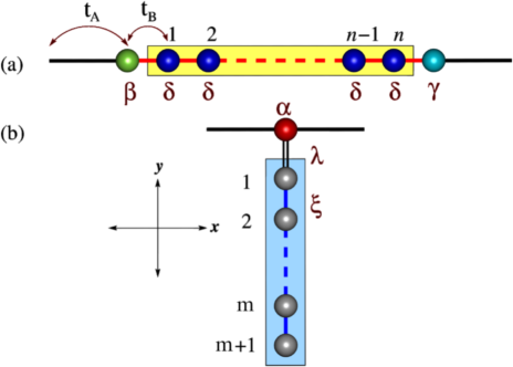
Figure 1: (Color online) Basic structural units for the off-diagonally disordered chains. The black and red bonds correspond to the hopping integrals $t_{A}$ and $t_{B}$. The double bond corresponds to the backbone-side cluster coupling $\lambda$ and $\xi$ represents the hopping integral in the bulk of the hanging atomic cluster.

In this communication we address ourselves this particular question. A one dimensional chain is grown along the $x$-direction by placing two basic structural units $\beta\delta^{n}\gamma$ and $\alpha$, with an atomic cluster side-coupled to the $\alpha$-sites only (Fig. 1) in any desired arrangement, for example, in a completely random way or following any deterministically disordered (may be quasiperiodic) geometry.

The sites are named in the following way. The $\alpha$ site is flanked by two identical bonds $A$. The $\beta$ and $\gamma$ sites are flanked by $A$ on the left and $B$ on the right, and the other way round. The $\delta$ sites are flanked on either side by the bond of type $B$. The hopping integrals corresponding to these bonds are named as $t_{A}$ and $t_{B}$ respectively. The general character of the spectrum in such cases, as can be appreciated easily, will reflect localization of electronic states, exponential or power law, depending on the distribution.

The side-coupled clusters extend in the $y$-direction and introduces a quasi-one dimensionality, but only in the minimal way, and locally at an infinite subset of the atomic sites (of type $\alpha$) in the basic chain, henceforth referred to as the ‘backbone’. We work within the framework of the tight binding scheme, and with off-diagonal disorder only, that is, the on-site potential is assigned a constant value for all the sites, including those in the hanging clusters.

It is observed, quite contrary to the usual picture of Anderson localization [1], that a definite correlation between the numerical values of the hopping integrals along the backbone ($t_{A}$ and $t_{B}$), the backbone-cluster tunnel hopping amplitude ($\lambda$), and the intra-cluster hopping ($\xi$) can render any spectrum, namely, point or singular continuous in to an assembly of absolutely continuous subbands. The continuous subbands turn out to be populated with extended Bloch like states only, and this happens irrespective of the electron’s energy, in total contrast to the already existing results of the RDM class of lattices, where only a finite number of resonant eigenstates are observed arising out of a positionally correlated disorder. We provide a detailed analysis for a quasiperiodic copper mean lattice [30], but emphasize that, the observation is by no means, restricted to them.

Before we conclude this section, it may be appropriated to mention at this point that linear atomic chains with side-coupled atomic clusters, the so called Fano-Anderson defects [31] have drawn interest over the past years not only for their unusual localization and transport properties, mimicking to some extent, the branched polymers [32], but also for their suitability as models of waveguides [33], and observation of the Fano resonances in the electronic transport [34]. Experimental observation of Fano profile in the electronic transmission across a quantum wire with a side-coupled quantum dot [35] has strengthened the need for a detailed study of such systems. A strong point of interest in such studies has been the functionalization of the backbone by the hanging clusters, where the electronic states of the side-attachment interfere with the spectrum of the linear chain (the backbone) which gives rise to rich spectral features [36]. The present work, which allows for a coupling of the discrete eigenstates of the hanging cluster with the spectrum of the linear backbone offering a spectrum depending on its topography, could be of considerable interest to the experimentalists as well.

In what follows, we present the results. In the second and third section we provide the tight binding Hamiltonian to work with, and the basic scheme for engineering the continuous subbands in the energy spectrum. In the fourth section we discuss the case of a copper mean chain (CMC) and illustrates how the usual spectrum of a CMC gets converted into a three subband continuous pattern as we approach the resonance conditions. In fifth section we present the transmission coefficient of finite segments of CMC to corroborate the density of states profiles discussed in fourth section, and finally in the last section we draw our conclusion.

The model and the method. – The variety of atomic environments is already described in the introduction, with reference to Fig. 1. A typical lattice with an arbitrary arrangement of these units is illustrated in Fig. 2(a). The array is modeled by the standard tight binding Hamiltonian written in the Wannier basis as,

$$H=\sum_{i}\epsilon_{i}c_{i}^{\dagger}c_{i}+\sum_{\langle ij\rangle}\left(t_{ij}c_{i}^{\dagger}c_{j}+h.c.\right),$$ (1)

where the on-site potential $\epsilon_{i}$ at the vertices $\alpha$, $\beta$ and $\gamma$ is set equal to a constant, viz., $\epsilon_{\alpha}=\epsilon_{\beta}=\epsilon_{\gamma}=\epsilon$. The potential at every site of the side coupled cluster is designated chosen to be equal to $\epsilon$. The nearest neighbor hopping integral $t_{ij}=t_{A}$ or $t_{B}$ along the backbone, and depends on the character of the bond, $A$ or $B$ they represent. The tunnel hopping integral between an $\alpha$-site and the first site of the side-coupled cluster (shown by a double bond in Fig. 1) is $t_{ij}=\lambda$, while the intra-cluster hopping in the side-attachment is represented by $\xi$.

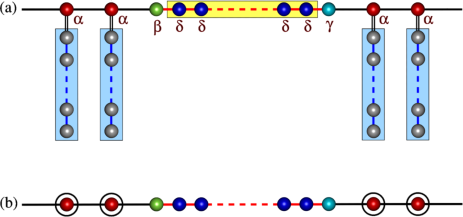
Figure 2: (Color online) (a) Basic structural units in Fig. 1 placed at random on the backbone. The hopping integrals $t_{A}$ and $t_{B}$ are represented by black and red lines along the backbone. (b) The hanging sites are decimated to generate an effectively one dimensional chain of modified $\alpha$ sites, the modification shown by encircling the relevant sites in (a).

The fundamental building blocks are placed in any desired pattern on a line (the backbone), for example, in a random or a quasiperiodic fashion. The geometry can easily be mapped onto a single linear chain comprising some effective atoms by decimating the cluster of atomic sites in the side-attachment to the $\alpha$-sites. This is illustrated in Fig. 2(b). The decimation process is easily implemented through the use of the set of difference equations

$$(E-\epsilon_{i})\psi_{i}=\sum_{\langle ij\rangle}t_{ij}\psi_{j},$$ (2)

for any $i$-th site in the side-coupled cluster. The resulting linear chain now has two kinds of blocks, one being the renormalized $\alpha$-site having an effective energy dependent on-site potential of the form

$$\tilde{\epsilon}_{\alpha}=\epsilon+\lambda^{2}\frac{U_{m}(y)}{\xi U_{m+1}(y)},$$ (3)

and the other is the original cluster of $\beta\delta^{n}\gamma$. In Eq. (3) $U_{m}(y)$ is the $m$-th order Chebyshev polynomial of the second kind and $y=(E-\epsilon)/2\xi$. The formulation of the equation (3) is shown in the Appendix in details.

Engineering the continuous subbands. – The effective linear chain depicted in Fig. 2(b) is described by the set of difference equations Eq. (2) with $\epsilon_{i}=\tilde{\epsilon}_{\alpha}$, $\epsilon_{\beta}$ or $\epsilon_{\gamma}$ (the latter two values being set equal to $\epsilon$) depending on the site. The hopping integral between nearest neighbors $t_{ij}$ are still $t_{A}$ or $t_{B}$ depending on the bond. The explicit equations for the three kinds of sites typically look like,

$$(E-\tilde{\epsilon}_{\alpha})\psi_{i} = t_{A}\psi_{i+1}+t_{A}\psi_{i-1},$$ (4a)

$$(E-\epsilon_{\beta})\psi_{i} = t_{B}\psi_{i+1}+t_{A}\psi_{i-1},$$ (4b)

$$(E-\epsilon_{\gamma})\psi_{i} = t_{A}\psi_{i+1}+t_{B}\psi_{i-1},$$ (4c)

where $i=\alpha$, $\beta$ or $\gamma$, as it comes. $\tilde{\epsilon}_{\alpha}$ is given by Eq. (3), while $\epsilon_{\beta}=\epsilon_{\gamma}=\epsilon$ as already explained.

The amplitude of the wave function at any $(i+1)$-th site is related to any arbitrary site through a simple product of $2\times 2$ transfer matrices, and is given by,

$$\left(\begin{array}[]{c}\psi_{i+1}\\ \psi_{i}\end{array}\right)=\bm{M_{i}}\!\cdot\!\bm{M_{i-1}}\!\cdots\!\bm{M_{2}}\!\cdot\!\bm{M_{1}}\left(\begin{array}[]{c}\psi_{1}\\ \psi_{0}\end{array}\right).$$ (5)

The above string of transfer matrices, written explicitly, is a product of two basic matrices, viz., $M_{\alpha}$ and $M_{\gamma\delta^{n}\beta}$ where,

$$\mbox{\boldmath$M_{\alpha}$}=\left(\begin{array}[]{cccc}2xR-\dfrac{\lambda^{2}U_{m}(y)}{\xi t_{A}U_{m+1}(y)}&-1\\ 1&0\end{array}\right),$$ (6c)

$$\mbox{\boldmath$M_{\gamma\delta^{n}\beta}$}=\left(\begin{array}[]{cccc}RU_{n+2}(x)&-\,U_{n+1}(x)\\ U_{n+1}(x)&-\,\dfrac{U_{n}(x)}{R}\end{array}\right).$$ (6f)

Here, $x=(E-\epsilon)/2t_{B}$, $y=(E-\epsilon)/2\xi$, and $R=t_{B}/t_{A}$. $U_{n}(x)$, as before, represents the $n$-th order Chebyshev polynomial of the second kind. The sequence of the two matrices $M_{\alpha}$ and $M_{\gamma\delta^{n}\beta}$ can be anything, aperiodic or

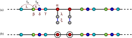
Figure 3: (Color online) (a) Portion of an infinite copper mean chain showing the four kinds of vertices along with the two bonds as shown. (b) Renormalization of the lattice in (a) into a purely 1-d chain.

random depending on how the clusters are arranged on the backbone.

It is straightforward to work out the commutator

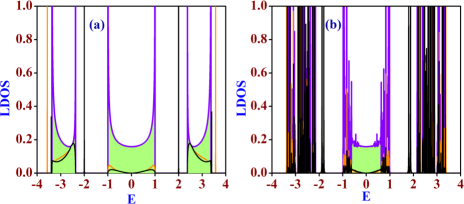
Figure 4: (Color online) Spectral landscape of a copper mean chain in (a) resonance condition, (b) $10\%$ deviation from the resonance condition. The initial values of the parameters in the resonance condition are $\epsilon_{\alpha}=\epsilon_{\beta}=\epsilon_{\gamma}=\epsilon_{\delta}=0$, $t_{A}=1$, $t_{B}=2$, $\lambda=\sqrt{3}$ and $\xi=2$. The dangling atoms also have the same on-site potentials as the four kinds of sites of CMC.

$[$$M_{\alpha}$$,\,$$M_{\gamma\delta^{n}\beta}$$]$, and see that the matrix elements of the commutator read, $[$$M_{\alpha}$$,\,$$M_{\gamma\delta^{n}\beta}$$]_{1,1}=0$ and, $[$$M_{\alpha}$$,\,$$M_{\gamma\delta^{n}\beta}$$]_{2,2}=0$, while,

$$\mbox{[\boldmath$M_{\alpha}$},\,\mbox{\boldmath$M_{\gamma\delta^{n}\beta}$}]_{1,2}=RU_{n+2}(x)-2xRU_{n+1}(x)+$$ (7)

$$\frac{U_{n}(x)}{R}+\frac{\lambda^{2}U_{n+1}(x)U_{m}(y)}{\xi t_{A}U_{m+1}(y)},$$

with $[$$M_{\alpha}$$,\,$$M_{\gamma\delta^{n}\beta}$$]_{2,1}=[$$M_{\alpha}$$,\,$$M_{\gamma\delta^{n}\beta}$$]_{1,2}$.

It is interesting to note that if we set $m=n$, that is, if the number of atoms in the side-coupled cluster becomes equal to $n+1$, one excess to the number of the $\delta$-sites in the cluster $\beta\delta^{n}\gamma$, the commutator $[$$M_{\alpha}$$,\,$$M_{\gamma\delta^{n}\beta}$$]=0$. In terms of the actual lattice it implies that the electronic spectrum will be insensitive to the arrangement of the clusters $\alpha$ (renormalized) and $\beta\delta^{n}\gamma$. Any disordered arrangement, deterministic or random, of these two different atomic clusters will then, in principle, will be indistinguishable from a perfectly periodic arrangement of an infinitely long string of $\alpha$-like sites and an infinite array of the $\beta\delta^{n}\gamma$ polymers.

A copper mean quasiperiodic chain as an example. – To check the arguments laid down so far, we fix, without loss of any generality, $n=1$, and construct a quasiperiodic copper mean chain (CMC) consisting of two ‘bonds’ $A$ and $B$, and following the recursive growth rule $A\rightarrow ABB$ and $B\rightarrow A$. The resulting CMC has isolated $\alpha$-type atoms flanked by two $A$-bonds on either side, and a cluster of $\beta\delta\gamma$ triplets, as shown in Fig. 3. For such a CMC we need to side-couple a two atom cluster to the $\alpha$-sites (as $m=n$ is the resonance condition).

As we now appreciate the original CMC, under the resonance condition, is equivalent to an infinite periodic array of the renormalized $\alpha$ sites (obtained after folding the hanging chain back into the backbone site) along with another periodic array of the $\beta\delta\gamma$ triplet. We now evaluate the local density of states (LDOS) at the renormalized (encircled) $\alpha$-chain and any site in the periodic $\beta\delta\gamma$ chain (Fig. 3(b)). The local densities of states are given, for these two infinite periodic lattices, and

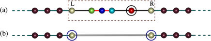
Figure 5: (Color online) A finite generation copper mean chain clamped between two semi-infinite ordered leads (solid brown circles).

for a given set of values of $\epsilon$, $\lambda$, $\xi$, $t_{A}$ and $t_{B}$, by $\rho_{00}^{\alpha}=1/(\pi\sqrt{Q_{\alpha}})$ and $\rho_{00}^{\beta}=1/(\pi\sqrt{Q_{\beta}})$ where

$$Q_{\alpha}=4t_{A}^{2}-\left[E-\epsilon-\frac{\lambda^{2}U_{m}(y)}{\xi U_{m+1}(y)}\right]^{2},$$ (8a)

$$Q_{\beta}=\frac{4t_{A}^{2}}{U_{n+1}^{2}(x)}$$

$$\quad-t_{B}^{2}\left[2x-\frac{1}{U_{n}^{2}(x)}\left(U_{n-1}(x)+\frac{R^{2}+U_{n}^{2}(x)}{R^{2}U_{n+1}(x)}\right)\right]^{2}.$$ (8b)

As soon as one sets $\lambda=\sqrt{t_{B}^{2}-t_{A}^{2}}$, $\xi=t_{B}$ and $m=n$ the LDOS of the two separate periodic chains become identical independent of energy, resulting in a complete overlap of the continuous subbands in the spectra of these individual chains under the above resonance condition.

This is illustrated sequentially in Fig. 4. In the first plot, viz., Fig. 4(a) we present the density of states under the resonance condition. The green shaded curves with violet outlines represent the absolutely continuous subbands, and arise out of the $\alpha$-sites. The LDOS from the $\beta$, $\delta$ and the $\gamma$ sites cover up the same subbands as well. The envelops of the black and the orange lines that fall within the green shaded zones provide the LDOS at the middle and the end sites in the side-coupled two-atom clusters. Thus there is a complete overlap of the absolutely continuous subbands arising out of the each individual lattice points. Of course, one should observe the appearance of isolated, pinned localized eigenstates, marked by the black and the orange spikes in Fig. 4(a) which occur at $E=\pm 2$ and $\pm 3.57$. These are the contributions coming from the top and the middle atoms in the side-coupled clusters.

Fig. 4(b) presents results for the LDOS as we deviate from the resonance condition by ten percent. The central continuum practically remains undislodged, while we observe dense packing of eigenstates in the subbands at the flanks. We have checked carefully the flow of the hopping integrals under the RSRG iterations [30] for a wide collection of energies, placed densely in all such regions. For every energy belonging to the continuum zone the hopping integrals keep on oscillating for indefinite number of iterations, without converging to zero, indicating complete extendedness of the corresponding eigenfunctions. On the other hand, for $E=\pm 2$ and $\pm 3.57$, the hopping integrals $t_{A}$ and $t_{B}$ flow to zero under iteration very quickly. As we get non-zero densities of states for these energies, the only conclusion that can be drawn is that, such states are localized. The small number of iterations indicate practically zero overlap of the corresponding wavefunction with the neighboring sites. This gives us confidence to conclude that such states must be pinned at some of the atomic sites in the system, likely places being the hanging clusters themselves. This has been cross checked by observing the flow of the trace-map, that has been used as a diagnostic tool for localization in aperiodic systems [37]. For eigenvalues residing within the absolutely continuous bands, the trace of the transfer matrix of any $l$-th generation CMC remains bounded by $2$ [37], while for the localized states it is not. This observations indicate that a possible experimental growth of such systems can indeed test the robustness of the conclusions drawn so far.

Two terminal transport. – The two terminal transmission coefficient is easily evaluated following the standard

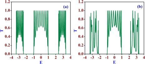
Figure 6: (Color online) Transmission spectrum of a $5$-th generation copper mean chain in (a) resonance condition, (b) $10\%$ deviation from the resonance condition. The initial values of the parameters in the resonance condition are $\epsilon_{\alpha}=\epsilon_{\beta}=\epsilon_{\gamma}=\epsilon_{\delta}=0$, $t_{A}=1$, $t_{B}=2$, $\lambda=\sqrt{3}$ and $\xi=2$. The dangling atoms also have the same on-site potentials as the four kinds of sites of CMC. The initial values of the lead parameters are respectively $\epsilon_{0}=0$ and $t_{0}=2$.

prescription [38]. A finite generation CMC is clamped between two semi-infinite ordered leads (as shown in Fig. 5) which is characterized by a constant on-site potential $\epsilon_{0}$ and a constant nearest neighbor hopping integral $t_{0}$. The segment of CMC clamped between the leads is successively renormalized with the help of the RSRG recursion relations for the on-site potentials and the hopping integrals in the CMC exploiting a reversal of its growth rule. Without loss of generality, we work out the transmission coefficient for odd generation CMC’s which ‘end’ with an $A$ bond. To achieve a uniform scaling of the end atoms we renormalize the chain by the reverse transformation $ABBAA\rightarrow A^{\prime}$ and $ABB\rightarrow B^{\prime}$. This makes a $(2n+1)$-th generation CMC get folded into the $1$st generation chain (comprising a single $A$-bond) after $n$ steps of decimation. The recursion relations for the potentials and the hopping integrals are then given by,

$$\tilde{\epsilon}_{\alpha,n+1}=\tilde{\epsilon}_{\alpha,n}+\frac{t_{A,n}^{2}\chi_{2,n}}{\chi_{3,n}}+\frac{t_{A,n}^{2}\sigma_{2,n}}{\sigma_{3,n}},$$ (9)

$$\epsilon_{\beta,n+1}=\tilde{\epsilon}_{\alpha,n}+\frac{t_{A,n}^{2}\sigma_{2,n}}{\sigma_{3,n}}+\frac{t_{A,n}^{2}(E-\epsilon_{\delta,n})}{\sigma_{1,n}},$$

$$\epsilon_{\gamma,n+1}=\epsilon_{\gamma,n}+\frac{t_{A,n}^{2}\chi_{2,n}}{\chi_{3,n}}+\frac{t_{B,n}^{2}(E-\epsilon_{\beta,n})}{\sigma_{1,n}},$$

$$\epsilon_{\delta,n}=\epsilon_{\gamma,n}+\frac{t_{B,n}^{2}(E-\epsilon_{\beta,n})}{\sigma_{1,n}}+\frac{t_{A,n}^{2}(E-\epsilon_{\delta,n})}{\sigma_{1,n}},$$

$$t_{A,n+1}=\frac{t_{A,n}^{3}t_{B,n}^{2}}{\chi_{3,n}},$$

$$t_{B,n+1}=\frac{t_{B,n}^{2}t_{A,n}}{\sigma_{1,n}}.$$

The ‘end’ sites $L$ and $R$ get renormalized following the rules,

$$\epsilon_{L,n+1}=\epsilon_{L,n}+\frac{t_{A,n}^{2}\chi_{2,n}}{\chi_{3,n}},$$ (10)

$$\epsilon_{R,n+1}=\epsilon_{R,n}+\frac{t_{A,n}^{2}\sigma_{2,n}}{\sigma_{3,n}}.$$

Here, $\chi_{2,n}=[(E-\epsilon_{\delta_{n}})\chi_{1,n}-t_{B,n}^{2}(E-\epsilon_{\alpha,n})]$, with $\chi_{1,n}=(E-\epsilon_{\gamma,n})(E-\epsilon_{\alpha,n})-t_{A,n}^{2}$. $\chi_{3,n}=[(E-\epsilon_{\beta,n})\chi_{2,n}-t_{B,n}^{2}\chi_{1,n}]$, $\sigma_{1,n}=(E-\epsilon_{\delta,n})(E-\epsilon_{\beta,n})-t_{B,n}^{2}$, $\sigma_{2,n}=(E-\epsilon_{\gamma,n})\sigma_{1,n}-t_{B,n}^{2}(E-\epsilon_{\beta,n})$, and, $\sigma_{3,n}=\sigma_{2,n}(E-\epsilon_{\alpha,n})-\sigma_{1,n}t_{A,n}^{2}$.

The two terminal transport coefficient of a $(2n+1)$-th generation CMC is then given by,

$$T=\dfrac{4\sin^{2}ka}{|\mathcal{P}|^{2}+|\mathcal{Q}|^{2}}.$$ (11)

$$\text{with}\quad\mathcal{P}=[(M_{12}-M_{21})+(M_{11}-M_{22})\cos ka]$$

$$\text{and}\quad\mathcal{Q}=[(M_{11}+M_{22})\sin ka],$$

where $M_{11}=(E-\epsilon_{R,n})(E-\epsilon_{L,n})/t_{0}t_{A,n}-t_{A,n}/t_{0}$, $M_{12}=-(E-\epsilon_{R,n})/t_{A,n}$, $M_{21}=(E-\epsilon_{L,n})/t_{A,n}$, and $M_{22}=-t_{0}/t_{A,n}$.

In Fig. 6 we exhibit the two terminal transport of a $5$-th generation CMC with the $\alpha$-sites attached with two-atom clusters. Three clear transmission windows are visible exactly over the energy ranges of the absolutely continuous subbands when resonance condition is enforced (Fig. 6(a)). This is at per with the expectation that these subbands are populated with extended eigenfunctions only. Interestingly, even with a ten percent deviation from the condition of resonance the transparent windows of transmission coefficient demonstrates the robustness of the result.

It is of interest to observe that, the renormalized potential $\tilde{\epsilon}_{\alpha}$ reduces to its bare scale value $\epsilon_{\alpha}=\epsilon$ for energy eigenvalues which are solutions of the equation $U_{m}(y)=0$. Each such energy values, which reside within the energy band of the semi-infinite leads, will give rise to a resonant electronic transmission. For these energies, the excursion of the propagating electron in the hanging clusters does not change the phase of the wavefunction. Similar issues, including the occurrence of the stop bands in between the absolute continua of the spectrum of a model quantum wire with side-coupled nanowires were discussed previously by Orellana et al. [39]

It is also important to appreciate that, the resonant transmission ($T=1$) seen in the present case is definitely caused by the fact that the transfer matrices across the clusters $\alpha$ and $\beta\delta^{n}\gamma$ commute irrespective of energy when we set the desired correlation between the hopping integrals, as mentioned already. This is to be contrasted with the case of, for example, the RDM, where under a resonance condition, the transfer matrix across a local pair of impurity atoms just turned out to be an identity matrix [24] at only a special value of the electron’s energy. In the present case, the commutation makes the lattice indistinguishable from a periodic array of the same scatterers. The transmission resonances thus result out of the phase coherence, as the electron is made to travel through the system.

Before we end this section, it is pertinent to remind the reader that the choice of a copper mean lattice is just for the sake of presenting analytically exact results. The condition of resonance, and it’s consequences, are by no means restricted to such a specific case, and definitely hold good for a completely random distribution of the clusters $\beta\delta^{n}\gamma$ and $\alpha$. Variants of the idea presented in this communication has already been tested with other geometries elsewhere [28].

Concluding remarks. – We have shown that suitably introducing minimal quasi-one dimensionality to a selected subset of atomic sites in an infinite linear chain one can obtain absolutely continuous spectrum in an off-diagonal model with random or any kind of deterministic disorder. This requires an appropriate correlation between the numerical values of a subset of the Hamiltonian parameters, in contradistinction with the conventional Anderson localization problem. The results indicate a possibility of manipulating a spectral crossover, if not an insulator to metal transition by tuning the hopping integrals appropriately. The result appears to be robust even when one deviates from the ideal conditions of resonance, a fact that may inspire experimentalists to undertake experiments with quantum wires, for example, with quantum dots coupled to it from a side.

$$\left(\begin{array}[]{c}\psi_{m+1}\\ \psi_{m}\end{array}\right)=\bm{M_{m}}\!\cdot\!\bm{M_{m-1}}\!\cdots\!\bm{M_{3}}\!\cdot\!\bm{M_{2}}\left(\begin{array}[]{c}\psi_{2}\\ \psi_{1}\end{array}\right).$$ (A. 1)

From which we must have,

$$\left(\begin{array}[]{c}\psi_{m+1}\\ \psi_{m}\end{array}\right)=\bm{M^{m-1}}\left(\begin{array}[]{c}\psi_{2}\\ \psi_{1}\end{array}\right).$$ (A. 2)

Thus, from the above equation, writing in terms of the Chebyshev polynomial we obtain,

$$\left(\begin{array}[]{c}\psi_{m+1}\\ \psi_{m}\end{array}\right)=\left(\begin{array}[]{cccc}2yU_{m-2}(y)-U_{m-3}(y)&-U_{m-2}(y)\\ U_{m-2}(y)&-U_{m-3}(y)\end{array}\right)\left(\begin{array}[]{c}\psi_{2}\\ \psi_{1}\end{array}\right).$$ (A. 3)

This obviously gives,

$$\left(\begin{array}[]{c}\psi_{m+1}\\ \psi_{m}\end{array}\right)=\left(\begin{array}[]{cccc}U_{m-1}(y)&-U_{m-2}(y)\\ U_{m-2}(y)&-U_{m-3}(y)\end{array}\right)\left(\begin{array}[]{c}\psi_{2}\\ \psi_{1}\end{array}\right).$$ (A. 4)

Here, $y=(E-\epsilon)/2\xi$. From Eq. (A. 4), we can write,

$$\psi_{m+1} = U_{m-1}(y)\psi_{2}-U_{m-2}(y)\psi_{1},$$ (A. 5a)

$$\psi_{m} = U_{m-2}(y)\psi_{2}-U_{m-3}(y)\psi_{1}.$$ (A. 5b)

Now, if we write down the difference equation for the $(m+1)$-th atom in the hanging cluster, we will get,

$$(E-\epsilon)\psi_{m+1}=\xi\psi_{m}.$$ (A. 6)

Therefore, substituting Eq. (A. 5) into the Eq. (A. 6) one can easily obtain after simplification the following expression.

$$\psi_{2}=\dfrac{U_{m-1}(y)}{U_{m}(y)}\psi_{1}.$$ (A. 7)

Now the difference equation for the $1$st atomic site in the hanging cluster reads as,

$$(E-\epsilon)\psi_{1}=\lambda\psi_{\alpha}+\xi\psi_{2}.$$ (A. 8)

By the use of Eq. (A. 7), one can obtain from Eq. (A. 8),

$$\psi_{1}=\dfrac{\lambda U_{m}(y)}{\xi U_{m+1}(y)}\psi_{\alpha}.$$ (A. 9)

Finally the difference equation for the $\alpha$-kind of site is given by,

$$(E-\epsilon)\psi_{\alpha}=\lambda\psi_{1}+t_{A}\sum_{j}\psi_{j}.$$ (A. 10)

From Eq. (A. 9) and Eq. (A. 10), we get the final form of the renormalized on-site potential as,

$$\tilde{\epsilon}_{\alpha}=\epsilon+\lambda^{2}\frac{U_{m}(y)}{\xi U_{m+1}(y)}.$$ (A. 11)

References

- [1] \NameAnderson P. W. \REVIEWPhys. Rev.10919581492.
- [2] \NameKramer B. MacKinnon A. \REVIEWRep. Prog. Phys.5619931469.
- [3] \NameAbrahams E., Anderson P. W., Licciardello D. C. Ramakrishnan T. V. \REVIEWPhys. Rev. Lett.421979673.
- [4] \NameRömer R. A. Schulz-Baldes H. \REVIEWEurophys. Lett.682004247.
- [5] \NameEilmes A., Römer R. A. Schreiber M. \REVIEWPhysica B296200146.
- [6] \NameRodríguez A. \REVIEWJ. Phys. A: Math. Gen.39200614303.
- [7] \NameRodriguez A., Vasquez L. J., Römer R. A. \REVIEWPhys. Rev. B782008195107.
- [8] \NameRodriguez A., Vasquez L. J., Slevin K. Römer R. A. \REVIEWPhys. Rev. B842011134209.
- [9] \NamePinski S. D., Schirmacher W. Römer R. A. \REVIEWEurophys. Lett.97201216007.
- [10] \NameYablonovitch E. \REVIEWPhys. Rev. Lett.5819872059.
- [11] \NameJohn S. \REVIEWPhys. Rev. Lett.5819872486.
- [12] \NameGilead Y., Verbin M. Silberberg Y. \REVIEWPhys. Rev. Lett.1152015133602.
- [13] \NameSvozilík J., Peřina J., Jr., Slevin K. Torres J. P. \REVIEWPhys. Rev. A892014053808.
- [14] \NameMontero de Espinosa F. R., Jiménez E. Torres M. \REVIEWPhys. Rev. Lett.8019981208.
- [15] \NameVasseur J. O., Deymier P. A., Frantziskonis G., Hong G., Djafari-Rouhani B. Dobrzynski L. \REVIEWJ. Phys.: Condens. Matter1019986051.
- [16] \NameBarinov I. O., Alodjants A. P. Arakelian S. M. \REVIEWQuantum Electron.392009685.
- [17] \NameTozer O. R. Barford W. \REVIEWPhys. Rev. B892014155434.
- [18] \NameTao A., Sinsermsuksaul P. Yang P. \REVIEWNat. Nanotechnol.22007435.
- [19] \NameChrist A., Ekinci Y., Solak H. H., Gippius N. A., Tikhodeev S. G. Martin O. J. F. \REVIEWPhys. Rev. B762007201405(R).
- [20] \NameRüting F. \REVIEWPhys. Rev. B832011115447.
- [21] \NameDamski B., Zakrzewski J., Santos L., Zoller P. Lewenstein M. \REVIEWPhys. Rev. Lett.912003080403.
- [22] \NameBilly J., Josse V., Zuo Z., Bernard A., Hambrecht B., Lugan P., Clément D., Sanchez-Palencia L., Bouyer P. Aspect A. \REVIEWNature (London)4532008891.
- [23] \NameRoati G., D’Errico C., Fallani L., Fattori M., Fort C., Zaccanti M., Modugno G., Modugno M. Inguscio M. \REVIEWNature (London)4532008895.
- [24] \NameDunlap D. H., Wu H-L. Phillips P. W. \REVIEWPhys. Rev. Lett.65199088.
- [25] \Namede Moura F. A. B. F. Lyra M. L. \REVIEWPhys. Rev. Lett.8119983735.
- [26] \NameSil S., Maiti S. K. Chakrabarti A. \REVIEWPhys. Rev. B782008113103.
- [27] \NameRodriguez A., Chakrabarti A. Römer R. A. \REVIEWPhys. Rev. B862012085119.
- [28] \NamePal B., Maiti S. K. Chakrabarti A. \REVIEWEurophys. Lett.102201317004.
- [29] \NamePal B. Chakrabarti A. \REVIEWPhys. Lett. A37820142782.
- [30] \NameSil S., Karmakar S. N., Moitra R. K. Chakrabarti A. \REVIEWPhys. Rev. B4819934192(R).
- [31] \NameMahan G. D. \BookMany-Particle Physics \PublPlenum Press, New York \Year1993.
- [32] \NameGuinea F. Vergés J. A. \REVIEWPhys. Rev. B351987979.
- [33] \NameMiroshnichenko A. E. Kivshar Y. S. \REVIEWPhys. Rev. E722005056611.
- [34] \NameMiroshnichenko A. E., Flach S. Kivshar Y. S. \REVIEWRev. Mod. Phys.8220102257.
- [35] \NameKobayashi K., Aikawa H., Sano A., Katsumoto S. Iye Y. \REVIEWPhys. Rev. B702004035319.
- [36] \NameFarchioni R., Grosso G. Parravicini G. P. \REVIEWPhys. Rev. B852012165115.
- [37] \NameNaumis G. G. \REVIEWJ. Phys.: Condens. Matter1520035969.
- [38] \NameStone A. D., Joannopoulos J. D. Chadi D. J. \REVIEWPhys. Rev. B2419815583.
- [39] \NameOrellana P. A., Guevara M. L. Ladron de, Dominguez-Adame F. Gomez I. \REVIEWPhys. Status Solidi C12004S50.