Successor Features for
Transfer in Reinforcement Learning

Abstract

Transfer in reinforcement learning refers to the notion that generalization should occur not only within a task but also across tasks. We propose a transfer framework for the scenario where the reward function changes between tasks but the environment’s dynamics remain the same. Our approach rests on two key ideas: successor features, a value function representation that decouples the dynamics of the environment from the rewards, and generalized policy improvement, a generalization of dynamic programming’s policy improvement operation that considers a set of policies rather than a single one. Put together, the two ideas lead to an approach that integrates seamlessly within the reinforcement learning framework and allows the free exchange of information across tasks. The proposed method also provides performance guarantees for the transferred policy even before any learning has taken place. We derive two theorems that set our approach in firm theoretical ground and present experiments that show that it successfully promotes transfer in practice, significantly outperforming alternative methods in a sequence of navigation tasks and in the control of a simulated robotic arm.

Abstract

In this supplement we give details of the theory and experiments that had to be left out of the main paper due to the space limit. For the convenience of the reader the statements of the theoretical results are reproduced before the respective proofs. We also provide a thorough description of the protocol used to carry out our experiments, present details of the algorithms, including their pseudo-code, and report additional empirical analysis that could not be included in the paper. The numbering of sections, equations, and figures resume that used in the main paper, so we refer to these elements as if paper and supplement were a single document. We also cite references listed in the main paper.

1 Introduction

Reinforcement learning (RL) provides a framework for the development of situated agents that learn how to behave while interacting with the environment [21]. The basic RL loop is defined in an abstract way so as to capture only the essential aspects of this interaction: an agent receives observations and selects actions to maximize a reward signal. This setup is generic enough to describe tasks of different levels of complexity that may unroll at distinct time scales. For example, in the task of driving a car, an action can be to turn the wheel, make a right turn, or drive to a given location.

Clearly, from the point of view of the designer, it is desirable to describe a task at the highest level of abstraction possible. However, by doing so one may overlook behavioral patterns and inadvertently make the task more difficult than it really is. The task of driving to a location clearly encompasses the subtask of making a right turn, which in turn encompasses the action of turning the wheel. In learning how to drive an agent should be able to identify and exploit such interdependencies. More generally, the agent should be able to break a task into smaller subtasks and use knowledge accumulated in any subset of those to speed up learning in related tasks. This process of leveraging knowledge acquired in one task to improve performance on other tasks is called transfer [25, 11].

In this paper we look at one specific type of transfer, namely, when subtasks correspond to different reward functions defined in the same environment. This setup is flexible enough to allow transfer to happen at different levels. In particular, by appropriately defining the rewards one can induce different task decompositions. For instance, the type of hierarchical decomposition involved in the driving example above can be induced by changing the frequency at which rewards are delivered: a positive reinforcement can be given after each maneuver that is well executed or only at the final destination. Obviously, one can also decompose a task into subtasks that are independent of each other or whose dependency is strictly temporal (that is, when tasks must be executed in a certain order but no single task is clearly “contained” within another).

The types of task decomposition discussed above potentially allow the agent to tackle more complex problems than would be possible were the tasks modeled as a single monolithic challenge. However, in order to apply this divide-and-conquer strategy to its full extent the agent should have an explicit mechanism to promote transfer between tasks. Ideally, we want a transfer approach to have two important properties. First, the flow of information between tasks should not be dictated by a rigid diagram that reflects the relationship between the tasks themselves, such as hierarchical or temporal dependencies. On the contrary, information should be exchanged across tasks whenever useful. Second, rather than being posed as a separate problem, transfer should be integrated into the RL framework as much as possible, preferably in a way that is almost transparent to the agent.

In this paper we propose an approach for transfer that has the two properties above. Our method builds on two conceptual pillars that complement each other. The first is a generalization of Dayan’s [7] successor representation. As the name suggests, in this representation scheme each state is described by a prediction about the future occurrence of all states under a fixed policy. We present a generalization of Dayan’s idea which extends the original scheme to continuous spaces and also facilitates the use of approximation. We call the resulting scheme successor features. As will be shown, successor features lead to a representation of the value function that naturally decouples the dynamics of the environment from the rewards, which makes them particularly suitable for transfer.

The second pillar of our framework is a generalization of Bellman’s [3] classic policy improvement theorem that extends the original result from one to multiple decision policies. This novel result shows how knowledge about a set of tasks can be transferred to a new task in a way that is completely integrated within RL. It also provides performance guarantees on the new task before any learning has taken place, which opens up the possibility of constructing a library of “skills” that can be reused to solve previously unseen tasks. In addition, we present a theorem that formalizes the notion that an agent should be able to perform well on a task if it has seen a similar task before—something clearly desirable in the context of transfer. Combined, the two results above not only set our approach in firm ground but also outline the mechanics of how to actually implement transfer. We build on this knowledge to propose a concrete method and evaluate it in two environments, one encompassing a sequence of navigation tasks and the other involving the control of a simulated two-joint robotic arm.

2 Background and problem formulation

As usual, we assume that the interaction between agent and environment can be modeled as a Markov decision process (MDP, Puterman, [19]). An MDP is defined as a tuple $M\equiv(\mathcal{S},\mathcal{A},p,R,\gamma)$. The sets $\mathcal{S}$ and $\mathcal{A}$ are the state and action spaces, respectively; here we assume that $\mathcal{S}$ and $\mathcal{A}$ are finite whenever such an assumption facilitates the presentation, but most of the ideas readily extend to continuous spaces. For each $s\in\mathcal{S}$ and $a\in\mathcal{A}$ the function $p(\cdot|s,a)$ gives the next-state distribution upon taking action $a$ in state $s$. We will often refer to $p(\cdot|s,a)$ as the dynamics of the MDP. The reward received at transition $s\xrightarrow{a}s^{\prime}$ is given by the random variable $R(s,a,s^{\prime})$; usually one is interested in the expected value of this variable, which we will denote by $r(s,a,s^{\prime})$ or by $r(s,a)=\mathrm{E}_{S^{\prime}\sim p(\cdot|s,a)}[r(s,a,S^{\prime})]$. The discount factor $\gamma\in[0,1)$ gives smaller weights to future rewards.

The objective of the agent in RL is to find a policy $\pi$—a mapping from states to actions—that maximizes the expected discounted sum of rewards, also called the return $G_{t}=\sum_{i=0}^{\infty}\gamma^{i}R_{t+i+1},$ where $R_{t}=R(S_{t},A_{t},S_{t+1})$. One way to address this problem is to use methods derived from dynamic programming (DP), which heavily rely on the concept of a value function [19]. The action-value function of a policy $\pi$ is defined as

$$Q^{\pi}(s,a)\equiv\mathrm{E}^{\pi}\left[G_{t}\,|\,S_{t}=s,A_{t}=a\right],$$ (1)

where $\mathrm{E}^{\pi}[\cdot]$ denotes expected value when following policy $\pi$. Once the action-value function of a particular policy $\pi$ is known, we can derive a new policy $\pi^{\prime}$ which is greedy with respect to $Q^{\pi}(s,a)$, that is, $\pi^{\prime}(s)\in\mathrm{argmax}_{a}Q^{\pi}(s,a)$. Policy $\pi^{\prime}$ is guaranteed to be at least as good as (if not better than) policy $\pi$. The computation of $Q^{\pi}(s,a)$ and $\pi^{\prime}$, called policy evaluation and policy improvement, define the basic mechanics of RL algorithms based on DP; under certain conditions their successive application leads to an optimal policy $\pi^{*}$ that maximizes the expected return from every $s\in\mathcal{S}$ [21].

In this paper we are interested in the problem of transfer, which we define as follows. Let $\mathcal{T},\mathcal{T}^{\prime}$ be two sets of tasks such that $\mathcal{T}^{\prime}\subset\mathcal{T}$, and let $t$ be any task. Then there is transfer if, after training on $\mathcal{T}$, the agent always performs as well or better on task $t$ than if only trained on $\mathcal{T}^{\prime}$. Note that $\mathcal{T}^{\prime}$ can be the empty set. In this paper a task will be defined as a specific instantiation of the reward function $R(s,a,s^{\prime})$ for a given MDP. In Section 4 we will revisit this definition and make it more formal.

3 Successor features

In this section we present the concept that will serve as a cornerstone for the rest of the paper. We start by presenting a simple reward model and then show how it naturally leads to a generalization of Dayan’s [7] successor representation (SR).

Suppose that the expected one-step reward associated with transition $(s,a,s^{\prime})$ can be computed as

$$r(s,a,s^{\prime})=\boldsymbol{\mathrm{\phi}}(s,a,s^{\prime})^{\top}\boldsymbol{\mathrm{w}},$$ (2)

where $\boldsymbol{\mathrm{\phi}}(s,a,s^{\prime})\in\mathbb{R}^{d}$ are features of $(s,a,s^{\prime})$ and $\boldsymbol{\mathrm{w}}\in\mathbb{R}^{d}$ are weights. Expression (2) is not restrictive because we are not making any assumptions about $\boldsymbol{\mathrm{\phi}}(s,a,s^{\prime})$: if we have $\phi_{i}(s,a,s^{\prime})=r(s,a,s^{\prime})$ for some $i$, for example, we can clearly recover any reward function exactly. To simplify the notation, let $\boldsymbol{\mathrm{\phi}}_{t}=\boldsymbol{\mathrm{\phi}}(s_{t},a_{t},s_{t+1})$. Then, by simply rewriting the definition of the action-value function in (1) we have

$$Q^{\pi}(s,a) =\mathrm{E}^{\pi}\left[r_{t+1}+\gamma r_{t+2}+...\,|\,S_{t}=s,A_{t}=a\right]$$

$$=\mathrm{E}^{\pi}\left[\boldsymbol{\mathrm{\phi}}_{t+1}^{\top}\boldsymbol{\mathrm{w}}+\gamma\boldsymbol{\mathrm{\phi}}_{t+2}^{\top}\boldsymbol{\mathrm{w}}+...\,|\,S_{t}=s,A_{t}=a\right]$$

$$=\mathrm{E}^{\pi}\left[{\textstyle\sum_{i=t}^{\infty}}\gamma^{i-t}\boldsymbol{\mathrm{\phi}}_{i+1}\,|\,S_{t}=s,A_{t}=a\right]^{\top}\boldsymbol{\mathrm{w}}=\boldsymbol{\mathrm{\psi}}^{\pi}(s,a)^{\top}\boldsymbol{\mathrm{w}}.$$ (3)

The decomposition (3) has appeared before in the literature under different names and interpretations, as discussed in Section 6. Since here we propose to look at (3) as an extension of Dayan’s [7] SR, we call $\boldsymbol{\mathrm{\psi}}^{\pi}(s,a)$ the successor features (SFs) of $(s,a)$ under policy $\pi$.

The i^th component of $\boldsymbol{\mathrm{\psi}}^{\pi}(s,a)$ gives the expected discounted sum of $\phi_{i}$ when following policy $\pi$ starting from $(s,a)$. In the particular case where $\mathcal{S}$ and $\mathcal{A}$ are finite and $\boldsymbol{\mathrm{\phi}}$ is a tabular representation of $\mathcal{S}\times\mathcal{A}\times\mathcal{S}$—that is, $\boldsymbol{\mathrm{\phi}}(s,a,s^{\prime})$ is a one-hot vector in $\mathbb{R}^{|\mathcal{S}|^{2}|\mathcal{A}|}$—$\boldsymbol{\mathrm{\psi}}^{\pi}(s,a)$ is the discounted sum of occurrences, under $\pi$, of each possible transition. This is essentially the concept of SR extended from the space $\mathcal{S}$ to the set $\mathcal{S}\times\mathcal{A}\times\mathcal{S}$ [7].

One of the contributions of this paper is precisely to generalize SR to be used with function approximation, but the exercise of deriving the concept as above provides insights already in the tabular case. To see this, note that in the tabular case the entries of $\boldsymbol{\mathrm{w}}\in\mathbb{R}^{|\mathcal{S}|^{2}|\mathcal{A}|}$ are the function $r(s,a,s^{\prime})$ and suppose that $r(s,a,s^{\prime})\neq 0$ in only a small subset $\mathcal{W}\subset\mathcal{S}\times\mathcal{A}\times\mathcal{S}$. From (2) and (3), it is clear that the cardinality of $\mathcal{W}$, and not of $\mathcal{S}\times\mathcal{A}\times\mathcal{S}$, is what effectively defines the dimension of the representation $\boldsymbol{\mathrm{\psi}}^{\pi}$, since there is no point in having $d>|\mathcal{W}|$. Although this fact is hinted at by Dayan [7], it becomes more apparent when we look at SR as a particular case of SFs.

SFs extend SR in two other ways. First, the concept readily applies to continuous state and action spaces without any modification. Second, by explicitly casting (2) and (3) as inner products involving feature vectors, SFs make it evident how to incorporate function approximation: as will be shown, these vectors can be learned from data.

The representation in (3) requires two components to be learned, $\boldsymbol{\mathrm{w}}$ and $\boldsymbol{\mathrm{\psi}}^{\pi}$. Since the latter is the expected discounted sum of $\boldsymbol{\mathrm{\phi}}$ under $\pi$, we must either be given $\boldsymbol{\mathrm{\phi}}$ or learn it as well. Note that approximating $r(s,a,s^{\prime})\approx\boldsymbol{\mathrm{\phi}}(s,a,s^{\prime})^{\top}\tilde{\boldsymbol{\mathrm{w}}}$ is a supervised learning problem, so we can use well-understood techniques from the field to learn $\tilde{\boldsymbol{\mathrm{w}}}$ (and potentially $\tilde{\boldsymbol{\mathrm{\phi}}}$, too) [9]. As for $\boldsymbol{\mathrm{\psi}}^{\pi}$, we note that

$$\boldsymbol{\mathrm{\psi}}^{\pi}(s,a) =\boldsymbol{\mathrm{\phi}}_{t+1}+\gamma E^{\pi}[\boldsymbol{\mathrm{\psi}}^{\pi}(S_{t+1},\pi(S_{t+1}))\,|\,S_{t}=s,A_{t}=a],$$ (4)

that is, SFs satisfy a Bellman equation in which $\phi_{i}$ play the role of rewards—something also noted by Dayan [7] regarding SR. Therefore, in principle any RL method can be used to compute $\boldsymbol{\mathrm{\psi}}^{\pi}$ [24].

The SFs $\boldsymbol{\mathrm{\psi}}^{\pi}$ summarize the dynamics induced by $\pi$ in a given environment. As shown in (3), this allows for a modular representation of $Q^{\pi}$ in which the MDP’s dynamics are decoupled from its rewards, which are captured by the weights $\boldsymbol{\mathrm{w}}$. One potential benefit of having such a decoupled representation is that only the relevant module must be relearned when either the dynamics or the reward changes, which may serve as an argument in favor of adopting SFs as a general approximation scheme for RL. However, in this paper we focus on a scenario where the decoupled value-function approximation provided by SFs is exploited to its full extent, as we discuss next.

4 Transfer via successor features

We now return to the discussion about transfer in RL. As described, we are interested in the scenario where all components of an MDP are fixed, except for the reward function. One way to formalize this model is through (2): if we suppose that $\boldsymbol{\mathrm{\phi}}\in\mathbb{R}^{d}$ is fixed, any $\boldsymbol{\mathrm{w}}\in\mathbb{R}^{d}$ gives rise to a new MDP. Based on this observation, we define

$$\mathcal{M}^{\phi}(\mathcal{S},\mathcal{A},p,\gamma)\equiv\{M(\mathcal{S},\mathcal{A},p,r,\gamma)\;|\;r(s,a,s^{\prime})=\boldsymbol{\mathrm{\phi}}(s,a,s^{\prime})^{\top}\boldsymbol{\mathrm{w}}\},$$ (5)

that is, $\mathcal{M}^{\phi}$ is the set of MDPs induced by $\boldsymbol{\mathrm{\phi}}$ through all possible instantiations of $\boldsymbol{\mathrm{w}}$. Since what differentiates the MDPs in $\mathcal{M}^{\phi}$ is essentially the agent’s goal, we will refer to $M_{i}\in\mathcal{M}^{\phi}$ as a task. The assumption is that we are interested in solving (a subset of) the tasks in the environment $\mathcal{M}^{\phi}$.

Definition (5) is a natural way of modeling some scenarios of interest. Think, for example, how the desirability of water or food changes depending on whether an animal is thirsty or hungry. One way to model this type of preference shifting is to suppose that the vector $\boldsymbol{\mathrm{w}}$ appearing in (2) reflects the taste of the agent at any given point in time [17]. Further in the paper we will present experiments that reflect this scenario. For another illustrative example, imagine that the agent’s goal is to produce and sell a combination of goods whose production line is relatively stable but whose prices vary considerably over time. In this case updating the price of the products corresponds to picking a new $\boldsymbol{\mathrm{w}}$. A slightly different way of motivating (5) is to suppose that the environment itself is changing, that is, the element $\boldsymbol{\mathrm{w}}_{i}$ indicates not only desirability, but also availability, of feature $\phi_{i}$.

In the examples above it is desirable for the agent to build on previous experience to improve its performance on a new setup. More concretely, if the agent knows good policies for the set of tasks $\mathcal{M}\equiv\{M_{1},M_{2},...,M_{n}\}$, with $M_{i}\in\mathcal{M}^{\phi}$, it should be able to leverage this knowledge to improve its behavior on a new task $M_{n+1}$—that is, it should perform better than it would had it been exposed to only a subset of the original tasks, $\mathcal{M}^{\prime}\subset\mathcal{M}$. We can assess the performance of an agent on task $M_{n+1}$ based on the value function of the policy followed after $\boldsymbol{\mathrm{w}}_{n+1}$ has become available but before any policy improvement has taken place in $M_{n+1}$. More precisely, suppose that an agent has been exposed to each one of the tasks $M_{i}\in\mathcal{M}^{\prime}$. Based on this experience, and on the new $\boldsymbol{\mathrm{w}}_{n+1}$, the agent computes a policy $\pi^{\prime}$ that will define its initial behavior in $M_{n+1}$. Now, if we repeat the experience replacing $\mathcal{M}^{\prime}$ with $\mathcal{M}$, the resulting policy $\pi$ should be such that $Q^{\pi}(s,a)\geq Q^{\pi^{\prime}}(s,a)$ for all $(s,a)\in\mathcal{S}\times\mathcal{A}$.

Now that our setup is clear we can start to describe our solution for the transfer problem discussed above. We do so in two stages. First, we present a generalization of DP’s notion of policy improvement whose interest may go beyond the current work. We then show how SFs can be used to implement this generalized form of policy improvement in an efficient and elegant way.

4.1 Generalized policy improvement

One of the fundamental results in RL is Bellman’s [3] policy improvement theorem. In essence, the theorem states that acting greedily with respect to a policy’s value function gives rise to another policy whose performance is no worse than the former’s. This is the driving force behind DP, and most RL algorithms that compute a value function are exploiting Bellman’s result in one way or another.

In this section we extend the policy improvement theorem to the scenario where the new policy is to be computed based on the value functions of a set of policies. We show that this extension can be done in a natural way, by acting greedily with respect to the maximum over the value functions available. Our result is summarized in the theorem below.

Theorem 1.

(Generalized Policy Improvement) Let $\pi_{1}$, $\pi_{2}$, …, $\pi_{n}$ be $n$ decision policies and let $\tilde{Q}^{\pi_{1}}$, $\tilde{Q}^{\pi_{2}}$, …, $\tilde{Q}^{\pi_{n}}$ be approximations of their respective action-value functions such that

$$|Q^{\pi_{i}}(s,a)-\tilde{Q}^{\pi_{i}}(s,a)|\leq\epsilon\,\text{ for all }s\in\mathcal{S},a\in\mathcal{A},\text{ and }i\in\{1,2,...,n\}.$$ (6)

Define

$${\pi}(s)\in\mathop{\mathrm{argmax}}_{a}\max_{i}\tilde{Q}^{\pi_{i}}(s,a).$$ (7)

Then,

$$Q^{\pi}(s,a)\geq\max_{i}Q^{\pi_{i}}(s,a)-\dfrac{2}{1-\gamma}\epsilon$$ (8)

for any $s\in\mathcal{S}$ and $a\in\mathcal{A}$, where $Q^{\pi}$ is the action-value function of ${\pi}$.

The proofs of our theoretical results are in the supplementary material. As one can see, our theorem covers the case where the policies’ value functions are not computed exactly, either because function approximation is used or because some exact algorithm has not be run to completion. This error is captured by $\epsilon$ in (6), which re-appears as a penalty term in the lower bound (8). Such a penalty is inherent to the presence of approximation in RL, and in fact it is identical to the penalty incurred in the single-policy case (see e.g. Bertsekas and Tsitsiklis’s Proposition 6.1 [5]).

In order to contextualize generalized policy improvement (GPI) within the broader scenario of DP, suppose for a moment that $\epsilon=0$. In this case Theorem 1 states that $\pi$ will perform no worse than all of the policies $\pi_{1}$, $\pi_{2},...,\pi_{n}$. This is interesting because in general $\max_{i}Q^{\pi_{i}}$—the function used to induce $\pi$—is not the value function of any particular policy. It is not difficult to see that $\pi$ will be strictly better than all previous policies if no single policy dominates all other policies, that is, if $\mathrm{argmax}_{i}\max_{a}\tilde{Q}^{\pi_{i}}(s,a)\cap\mathrm{argmax}_{i}\max_{a}\tilde{Q}^{\pi_{i}}(s^{\prime},a)=\emptyset$ for some $s,s^{\prime}\in\mathcal{S}$. If one policy does dominate all others, GPI reduces to the original policy improvement theorem.

If we consider the usual DP loop, in which policies of increasing performance are computed in sequence, our result is not of much use because the most recent policy will always dominate all others. Another way of putting it is to say that after Theorem 1 is applied once adding the resulting $\pi$ to the set $\{\pi_{1}$, $\pi_{2},...,\pi_{n}\}$ will reduce the next improvement step to standard policy improvement, and thus the policies $\pi_{1}$, $\pi_{2},...,\pi_{n}$ can be simply discarded. There are however two situations in which our result may be of interest. One is when we have many policies $\pi_{i}$ being evaluated in parallel. In this case GPI provides a principled strategy for combining these policies. The other situation in which our result may be useful is when the underlying MDP changes, as we discuss next.

4.2 Generalized policy improvement with successor features

We start this section by extending our notation slightly to make it easier to refer to the quantities involved in transfer learning. Let $M_{i}$ be a task in $\mathcal{M}^{\phi}$ defined by $\boldsymbol{\mathrm{w}}_{i}\in\mathbb{R}^{d}$. We will use $\pi^{*}_{i}$ to refer to an optimal policy of MDP $M_{i}$ and use $Q^{{}_{\pi_{i}^{*}}}_{i}$ to refer to its value function. The value function of $\pi^{*}_{i}$ when executed in $M_{j}\in\mathcal{M}^{\phi}$ will be denoted by $Q^{{}_{\pi_{i}^{*}}}_{j}$.

Suppose now that an agent has computed optimal policies for the tasks $M_{1},M_{2},...,M_{n}\in\mathcal{M}^{\phi}$. Suppose further that when presented with a new task $M_{n+1}$ the agent computes $\{Q^{\pi_{1}^{*}}_{n+1},Q^{\pi_{2}^{*}}_{n+1},...,Q^{\pi_{n}^{*}}_{n+1}\}$, the evaluation of each $\pi^{*}_{i}$ under the new reward function induced by $\boldsymbol{\mathrm{w}}_{n+1}$. In this case, applying the GPI theorem to the newly-computed set of value functions will give rise to a policy that performs at least as well as a policy based on any subset of these, including the empty set. Thus, this strategy satisfies our definition of successful transfer.

There is a caveat, though. Why would one waste time computing the value functions of $\pi_{1}^{*},\pi^{*}_{2}$, …, $\pi_{n}^{*}$, whose performance in $M_{n+1}$ may be mediocre, if the same amount of resources can be allocated to compute a sequence of $n$ policies with increasing performance? This is where SFs come into play. Suppose that we have learned the functions $Q^{{}_{\pi_{i}^{*}}}_{i}$ using the representation scheme shown in (3). Now, if the reward changes to $r_{n+1}(s,a,s^{\prime})=\boldsymbol{\mathrm{\phi}}(s,a,s^{\prime})^{\top}\boldsymbol{\mathrm{w}}_{n+1}$, as long as we have $\boldsymbol{\mathrm{w}}_{n+1}$ we can compute the new value function of $\pi_{i}^{*}$ by simply making $Q^{{}_{\pi_{i}^{*}}}_{n+1}(s,a)=\boldsymbol{\mathrm{\psi}}^{{}_{\pi_{i}^{*}}}(s,a)^{\top}\boldsymbol{\mathrm{w}}_{n+1}$. This reduces the computation of all ${Q}^{{}_{\pi_{i}^{*}}}_{n+1}$ to the much simpler supervised problem of approximating $\boldsymbol{\mathrm{w}}_{n+1}$.

Once the functions ${Q}^{{}_{\pi_{i}^{*}}}_{n+1}$ have been computed, we can apply GPI to derive a policy $\pi$ whose performance on $M_{n+1}$ is no worse than the performance of $\pi_{1}^{*},\pi^{*}_{2},...,\pi^{*}_{n}$ on the same task. A question that arises in this case is whether we can provide stronger guarantees on the performance of $\pi$ by exploiting the structure shared by the tasks in $\mathcal{M}^{\phi}$. The following theorem answers this question in the affirmative.

Theorem 2.

Let $M_{i}\in\mathcal{M}^{\phi}$ and let $Q^{{}_{\pi_{j}^{*}}}_{i}$ be the action-value function of an optimal policy of $M_{j}\in\mathcal{M}^{\phi}$ when executed in $M_{i}$. Given approximations $\{\tilde{Q}^{\pi_{1}^{*}}_{i},\tilde{Q}^{\pi_{2}^{*}}_{i},...,\tilde{Q}^{\pi_{n}^{*}}_{i}\}$ such that

$$\left|Q^{{}_{\pi_{j}^{*}}}_{i}(s,a)-\tilde{Q}^{{}_{\pi_{j}^{*}}}_{i}(s,a)\right|\leq\epsilon$$ (9)

for all $s\in\mathcal{S}$, $a\in\mathcal{A}$, and $j\in\{1,2,...,n\}$, let $\pi(s)\in\mathop{\mathrm{argmax}}_{a}\max_{j}\tilde{Q}^{{}_{\pi_{j}^{*}}}_{i}(s,a).$ Finally, let $\boldsymbol{\mathrm{\phi}}_{\max}=\max_{s,a}||\boldsymbol{\mathrm{\phi}}(s,a)||$, where $||\cdot||$ is the norm induced by the inner product adopted. Then,

$$Q^{{}_{\pi_{i}^{*}}}_{i}(s,a)-Q^{\pi}_{i}(s,a)\leq\dfrac{2}{1-\gamma}\left(\boldsymbol{\mathrm{\phi}}_{\max}\,\mathrm{min}_{j}||\boldsymbol{\mathrm{w}}_{i}-\boldsymbol{\mathrm{w}}_{j}||+\epsilon\right).$$ (10)

Note that we used $M_{i}$ rather than $M_{n+1}$ in the theorem’s statement to remove any suggestion of order among the tasks. Theorem 2 is a specialization of Theorem 1 for the case where the set of value functions used to compute $\pi$ are associated with tasks in the form of (5). As such, it provides stronger guarantees: instead of comparing the performance of $\pi$ with that of the previously-computed policies $\pi_{j}$, Theorem 2 quantifies the loss incurred by following $\pi$ as opposed to one of $M_{i}$’s optimal policies.

As shown in (10), the loss $Q^{{}_{\pi_{i}^{*}}}_{i}(s,a)-Q^{\pi}_{i}(s,a)$ is upper-bounded by two terms. The term $2\boldsymbol{\mathrm{\phi}}_{\max}\mathrm{min}_{j}||\boldsymbol{\mathrm{w}}_{i}-\boldsymbol{\mathrm{w}}_{j}||/(1-\gamma)$ is of more interest here because it reflects the structure of $\mathcal{M}^{\phi}$. This term is a multiple of the distance between $\boldsymbol{\mathrm{w}}_{i}$, the vector describing the task we are currently interested in, and the closest $\boldsymbol{\mathrm{w}}_{j}$ for which we have computed a policy. This formalizes the intuition that the agent should perform well in task $\boldsymbol{\mathrm{w}}_{i}$ if it has solved a similar task before. More generally, the term in question relates the concept of distance in $\mathbb{R}^{d}$ with difference in performance in $\mathcal{M}^{\phi}$. Note that this correspondence depends on the specific set of features $\boldsymbol{\mathrm{\phi}}$ used, which raises the interesting question of how to define $\boldsymbol{\mathrm{\phi}}$ such that tasks that are close in $\mathbb{R}^{d}$ induce policies that are also similar in some sense. Regardless of how exactly $\boldsymbol{\mathrm{\phi}}$ is defined, the bound (10) allows for powerful extrapolations. For example, by covering the relevant subspace of $\mathbb{R}^{d}$ with balls of appropriate radii centered at $\boldsymbol{\mathrm{w}}_{j}$ we can provide performance guarantees for any task $\boldsymbol{\mathrm{w}}$ [14]. This corresponds to building a library of options (or “skills”) that can be used to solve any task in a (possibly infinite) set [22]. In Section 5 we illustrate this concept with experiments.

Although Theorem 2 is inexorably related to the characterization of $\mathcal{M}^{\phi}$ in (5), it does not depend on the definition of SFs in any way. Here SFs are the mechanism used to efficiently apply the protocol suggested by Theorem 2. When SFs are used the value function approximations are given by $\tilde{Q}^{{}_{\pi_{j}^{*}}}_{i}(s,a)=\tilde{\boldsymbol{\mathrm{\psi}}}^{{}_{\pi_{j}^{*}}}(s,a)^{\top}\tilde{\boldsymbol{\mathrm{w}}}_{i}$. The modules $\tilde{\boldsymbol{\mathrm{\psi}}}^{{}_{\pi_{j}^{*}}}$ are computed and stored when the agent is learning the tasks $M_{j}$; when faced with a new task $M_{i}$ the agent computes an approximation of $\boldsymbol{\mathrm{w}}_{i}$, which is a supervised learning problem, and then uses the GPI policy $\pi$ defined in Theorem 2 to learn $\tilde{\boldsymbol{\mathrm{\psi}}}^{{}_{\pi_{i}^{*}}}$. Note that we do not assume that either ${\boldsymbol{\mathrm{\psi}}}^{{}_{\pi_{j}^{*}}}$ or $\boldsymbol{\mathrm{w}}_{i}$ is computed exactly: the effect of errors in $\tilde{\boldsymbol{\mathrm{\psi}}}^{{}_{\pi_{j}^{*}}}$ and $\tilde{\boldsymbol{\mathrm{w}}}_{i}$ are accounted for by the term $\epsilon$ appearing in (9). As shown in (10), if $\epsilon$ is small and the agent has seen enough tasks the performance of $\pi$ on $M_{i}$ should already be good, which suggests it may also speed up the process of learning $\tilde{\boldsymbol{\mathrm{\psi}}}^{{}_{\pi_{i}^{*}}}$.

Interestingly, Theorem 2 also provides guidance for some practical algorithmic choices. Since in an actual implementation one wants to limit the number of SFs $\tilde{\boldsymbol{\mathrm{\psi}}}^{{}_{\pi_{j}^{*}}}$ stored in memory, the corresponding vectors $\tilde{\boldsymbol{\mathrm{w}}}_{j}$ can be used to decide which ones to keep. For example, one can create a new $\tilde{\boldsymbol{\mathrm{\psi}}}^{{}_{\pi_{i}^{*}}}$ only when $\mathrm{min}_{j}||\tilde{\boldsymbol{\mathrm{w}}}_{i}-\tilde{\boldsymbol{\mathrm{w}}}_{j}||$ is above a given threshold; alternatively, once the maximum number of SFs has been reached, one can replace $\tilde{\boldsymbol{\mathrm{\psi}}}^{{}_{\pi_{k}^{*}}}$, where $k=\mathrm{argmin}_{j}||\tilde{\boldsymbol{\mathrm{w}}}_{i}-\tilde{\boldsymbol{\mathrm{w}}}_{j}||$ (here $\boldsymbol{\mathrm{w}}_{i}$ is the current task).

5 Experiments

In this section we present our main experimental results. Additional details, along with further results and analysis, can be found in Appendix B of the supplementary material.

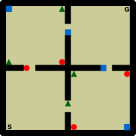
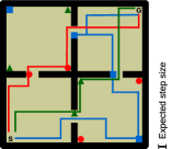
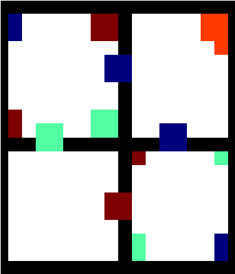
The first environment we consider involves navigation tasks defined over a two-dimensional continuous space composed of four rooms (Figure 1). The agent starts in one of the rooms and must reach a goal region located in the farthest room. The environment has objects that can be picked up by the agent by passing over them. Each object belongs to one of three classes determining the associated reward. The objective of the agent is to pick up the “good” objects and navigate to the goal while avoiding “bad” objects. The rewards associated with object classes change at every $20\,000$ transitions, giving rise to very different tasks (Figure 1). The goal is to maximize the sum of rewards accumulated over a sequence of $250$ tasks, with each task’s rewards sampled uniformly from $[-1,1]^{3}$.

Figure 1: Environment layout and some examples of optimal trajectories associated with specific tasks. The shapes of the objects represent their classes; ‘S’ is the start state and ‘G’ is the goal.

We defined a straightforward instantiation of our approach in which both $\tilde{\boldsymbol{\mathrm{w}}}$ and $\tilde{\boldsymbol{\mathrm{\psi}}}^{\pi}$ are computed incrementally in order to minimize losses induced by (2) and (4). Every time the task changes the current $\tilde{\boldsymbol{\mathrm{\psi}}}^{\pi_{i}}$ is stored and a new $\tilde{\boldsymbol{\mathrm{\psi}}}^{\pi_{i+1}}$ is created. We call this method SFQL as a reference to the fact that SFs are learned through an algorithm analogous to $Q$-learning (QL)—which is used as a baseline in our comparisons [27]. As a more challenging reference point we report results for a transfer method called probabilistic policy reuse [8]. We adopt a version of the algorithm that builds on QL and reuses all policies learned. The resulting method, PRQL, is thus directly comparable to SFQL. The details of QL, PRQL, and SFQL, including their pseudo-codes, are given in Appendix B.

We compared two versions of SFQL. In the first one, called SFQL-$\boldsymbol{\mathrm{\phi}}$, we assume the agent has access to features $\boldsymbol{\mathrm{\phi}}$ that perfectly predict the rewards, as in (2). The second version of our agent had to learn an approximation $\tilde{\boldsymbol{\mathrm{\phi}}}\in\mathbb{R}^{h}$ directly from data collected by QL in the first $20$ tasks. Note that $h$ may not coincide with the true dimension of $\boldsymbol{\mathrm{\phi}}$, which in this case is $4$; we refer to the different instances of our algorithm as SFQL-$h$. The process of learning $\tilde{\boldsymbol{\mathrm{\phi}}}$ followed the multi-task learning protocol proposed by Caruana [6] and Baxter [2], and described in detail in Appendix B.

The results of our experiments can be seen in Figure 2. As shown, all versions of SFQL significantly outperform the other two methods, with an improvement on the average return of more than $100\%$ when compared to PRQL, which itself improves on QL by around $100\%$. Interestingly, SFQL-$h$ seems to achieve good overall performance faster than SFQL-$\phi$, even though the latter uses features that allow for an exact representation of the rewards. One possible explanation is that, unlike their counterparts $\phi_{i}$, the features $\tilde{\phi}_{i}$ are activated over most of the space $\mathcal{S}\times\mathcal{A}\times\mathcal{S}$, which results in a dense pseudo-reward signal that facilitates learning.

Figure 2: Average and cumulative return per task in the four-room domain. SFQL-$h$ receives no reward during the first $20$ tasks while learning $\tilde{\boldsymbol{\mathrm{\phi}}}$. Error-bands show one standard error over $30$ runs.

The second environment we consider is a set of control tasks defined in the MuJoCo physics engine [26]. Each task consists in moving a two-joint torque-controlled simulated robotic arm to a specific target location; thus, we refer to this environment as “the reacher domain.” We defined $12$ tasks, but only allowed the agents to train in $4$ of them (Figure 3c). This means that the agent must be able to perform well on tasks that it has never experienced during training.

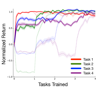
In order to solve this problem, we adopted essentially the same algorithm as above, but we replaced QL with Mnih et al.’s DQN—both as a baseline and as the basic engine underlying the SF agent [15]. The resulting method, which we call SFDQN, is an illustration of how our method can be naturally combined with complex nonlinear approximators such as neural networks. The features $\phi_{i}$ used by SFDQN are the negation of the distances to the center of the $12$ target regions. As usual in experiments of this type, we give the agents a description of the current task: for DQN the target coordinates are given as inputs, while for SFDQN this is provided as an one-hot vector $\boldsymbol{\mathrm{w}}_{t}\in\mathbb{R}^{12}$ [12]. Unlike in the previous experiment, in the current setup each transition was used to train all four $\tilde{\boldsymbol{\mathrm{\psi}}}^{\pi_{i}}$ through losses derived from (4). Here $\pi_{i}$ is the GPI policy on the i^th task: $\pi_{i}(s)\in\mathrm{argmax}_{a}\max_{j}\tilde{\boldsymbol{\mathrm{\psi}}}_{j}(s,a)^{\top}\boldsymbol{\mathrm{w}}_{i}$.

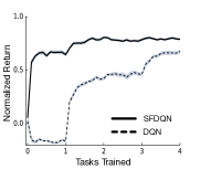
Results are shown in Figures 3a and 3b. Looking at the training curves, we see that whenever a task is selected for training SFDQN’s return on that task quickly improves and saturates at near-optimal performance. The interesting point to be noted is that, when learning a given task, SFDQN’s performance also improves in all other tasks, including the test ones, for which it does not have specialized policies. This illustrates how the combination of SFs and GPI can give rise to flexible agents able to perform well in any task of a set of tasks with shared dynamics—which in turn can be seen as both a form of temporal abstraction and a step towards more general hierarchical RL [22, 1].

(a) Performance on training tasks (faded dotted lines in the background are DQN’s results).

(b) Average performance on test tasks.

(c)   Colored and gray circles depict

training and test targets, respectively.

(b)

Figure 3: Normalized return on the reacher domain: ‘$1$’ corresponds to the average result achieved by DQN after learning each task separately and ‘$0$’ corresponds to the average performance of a randomly-initialized agent (see Appendix B for details). SFDQN’s results were obtained using the GPI policies $\pi_{i}(s)$ defined in the text. Shading shows one standard error over $30$ runs.

6 Related work

Mehta et al.’s [14] approach for transfer learning is probably the closest work to ours in the literature. There are important differences, though. First, Mehta et al. [14] assume that both $\boldsymbol{\mathrm{\phi}}$ and $\boldsymbol{\mathrm{w}}$ are always observable quantities provided by the environment. They also focus on average reward RL, in which the quality of a decision policy can be characterized by a single scalar. This reduces the process of selecting a policy for a task to one decision made at the outset, which is in clear contrast with GPI.

The literature on transfer learning has other methods that relate to ours [25, 11]. Among the algorithms designed for the scenario considered here, two approaches are particularly relevant because they also reuse old policies. One is Fernández et al.’s [8] probabilistic policy reuse, adopted in our experiments and described in Appendix B. The other approach, by Bernstein [4], corresponds to using our method but relearning all $\tilde{\boldsymbol{\mathrm{\psi}}}^{\pi_{i}}$ from scratch at each new task.

When we look at SFs strictly as a representation scheme, there are clear similarities with Littman et al.’s [13] predictive state representation (PSR). Unlike SFs, though, PSR tries to summarize the dynamics of the entire environment rather than of a single policy $\pi$. A scheme that is perhaps closer to SFs is the value function representation sometimes adopted in inverse RL [18].

SFs are also related to Sutton et al.’s [23] general value functions (GVFs), which extend the notion of value function to also include “pseudo-rewards.” If we see $\phi_{i}$ as a pseudo-reward, $\psi^{\pi}_{i}(s,a)$ becomes a particular case of GVF. Beyond the technical similarities, the connection between SFs and GVFs uncovers some principles underlying both lines of work that, when contrasted, may benefit both. On one hand, Sutton et al.’s [23] and Modayil et al.’s [16] hypothesis that relevant knowledge about the world can be expressed in the form of many predictions naturally translates to SFs: if $\boldsymbol{\mathrm{\phi}}$ is expressive enough, the agent should be able to represent any relevant reward function. Conversely, SFs not only provide a concrete way of using this knowledge, they also suggest a possible criterion to select the pseudo-rewards $\phi_{i}$, since ultimately we are only interested in features that help in the approximation $\boldsymbol{\mathrm{\phi}}(s,a,s^{\prime})^{\top}\tilde{\boldsymbol{\mathrm{w}}}\approx r(s,a,s^{\prime})$.

Another generalization of value functions that is related to SFs is Schaul et al.’s [20] universal value function approximators (UVFAs). UVFAs extend the notion of value function to also include as an argument an abstract representation of a “goal,” which makes them particularly suitable for transfer. The function $\max_{j}\tilde{\boldsymbol{\mathrm{\psi}}}^{{}_{\pi_{j}^{*}}}(s,a)^{\top}\tilde{\boldsymbol{\mathrm{w}}}$ used in our framework can be seen as a function of $s$, $a$, and $\tilde{\boldsymbol{\mathrm{w}}}$—the latter a generic way of representing a goal—, and thus in some sense this representation is a UVFA. The connection between SFs and UVFAs raises an interesting point: since under this interpretation $\tilde{\boldsymbol{\mathrm{w}}}$ is simply the description of a task, it can in principle be a direct function of the observations, which opens up the possibility of the agent determining $\tilde{\boldsymbol{\mathrm{w}}}$ even before seeing any rewards.

As discussed, our approach is also related to temporal abstraction and hierarchical RL: if we look at $\boldsymbol{\mathrm{\psi}}^{\pi}$ as instances of Sutton et al.’s [22] options, acting greedily with respect to the maximum over their value functions corresponds in some sense to planning at a higher level of temporal abstraction (that is, each $\boldsymbol{\mathrm{\psi}}^{\pi}(s,a)$ is associated with an option that terminates after a single step). This is the view adopted by Yao et al. [28], whose universal option model closely resembles our approach in some aspects (the main difference being that they do not do GPI).

Finally, there have been previous attempts to combine SR and neural networks. Kulkarni et al. [10] and Zhang et al. [29] propose similar architectures to jointly learn $\tilde{\boldsymbol{\mathrm{\psi}}}^{\pi}(s,a)$, $\tilde{\boldsymbol{\mathrm{\phi}}}(s,a,s^{\prime})$ and $\tilde{\boldsymbol{\mathrm{w}}}$. Although neither work exploits SFs for GPI, they both discuss other uses of SFs for transfer. In principle the proposed (or similar) architectures can also be used within our framework.

7 Conclusion

This paper builds on two concepts, both of which are generalizations of previous ideas. The first one is SFs, a generalization of Dayan’s [7] SR that extends the original definition from discrete to continuous spaces and also facilitates the use of function approximation. The second concept is GPI, formalized in Theorem 1. As the name suggests, this result extends Bellman’s [3] classic policy improvement theorem from a single to multiple policies.

Although SFs and GPI are of interest on their own, in this paper we focus on their combination to induce transfer. The resulting framework is an elegant extension of DP’s basic setting that provides a solid foundation for transfer in RL. As a complement to the proposed transfer approach, we derived a theoretical result, Theorem 2, that formalizes the intuition that an agent should perform well on a novel task if it has seen a similar task before. We also illustrated with a comprehensive set of experiments how the combination of SFs and GPI promotes transfer in practice.

We believe the proposed ideas lay out a general framework for transfer in RL. By specializing the basic components presented one can build on our results to derive agents able to perform well across a wide variety of tasks, and thus extend the range of environments that can be successfully tackled.

Appendix A Proofs of theoretical results

Theorem 1.

(Generalized Policy Improvement) Let $\pi_{1}$, $\pi_{2}$, …, $\pi_{n}$ be $n$ decision policies and let $\tilde{Q}^{\pi_{1}}$, $\tilde{Q}^{\pi_{2}}$, …, $\tilde{Q}^{\pi_{n}}$ be approximations of their respective action-value functions such that

$$|Q^{\pi_{i}}(s,a)-\tilde{Q}^{\pi_{i}}(s,a)|\leq\epsilon\,\text{ for all }s\in S,a\in A,\text{ and }i\in\{1,2,...,n\}.$$

Define

$${\pi}(s)\in\mathop{\mathrm{argmax}}_{a}\max_{i}\tilde{Q}^{\pi_{i}}(s,a).$$

Then,

$$Q^{\pi}(s,a)\geq\max_{i}Q^{\pi_{i}}(s,a)-\dfrac{2}{1-\gamma}\epsilon$$

for any $s\in S$ and any $a\in A$, where $Q^{\pi}$ is the action-value function of ${\pi}$.

Proof.

To simplify the notation, let

$$\begin{array}[]{ccc}Q_{\mathrm{max}}(s,a)=\max_{i}Q^{\pi_{i}}(s,a)&\text{ and }&\tilde{Q}_{\mathrm{max}}(s,a)=\max_{i}\tilde{Q}^{\pi_{i}}(s,a).\end{array}$$

We start by noting that for any $s\in S$ and any $a\in A$ the following holds:

$$|Q_{\mathrm{max}}(s,a)-\tilde{Q}_{\mathrm{max}}(s,a)|=|\max_{i}Q^{\pi_{i}}(s,a)-\max_{i}\tilde{Q}^{\pi_{i}}(s,a)|\leq\max_{i}|Q^{\pi_{i}}(s,a)-\tilde{Q}^{\pi_{i}}(s,a)|\leq\epsilon.$$

For all $s\in S$, $a\in A$, and $i\in\{1,2,...,n\}$ we have

$$T^{\pi}\tilde{Q}_{\mathrm{max}}(s,a) =r(s,a)+\gamma\sum_{s^{\prime}}p(s^{\prime}|s,a)\tilde{Q}_{\mathrm{max}}(s^{\prime},{\pi}(s^{\prime}))$$

$$=r(s,a)+\gamma\sum_{s^{\prime}}p(s^{\prime}|s,a)\max_{b}\tilde{Q}_{\mathrm{max}}(s^{\prime},b)$$

$$\geq r(s,a)+\gamma\sum_{s^{\prime}}p(s^{\prime}|s,a)\max_{b}Q_{\mathrm{max}}(s^{\prime},b)-\gamma\epsilon$$

$$\geq r(s,a)+\gamma\sum_{s^{\prime}}p(s^{\prime}|s,a)Q_{\mathrm{max}}(s^{\prime},\pi_{i}(s^{\prime}))-\gamma\epsilon$$

$$\geq r(s,a)+\gamma\sum_{s^{\prime}}p(s^{\prime}|s,a)Q^{\pi_{i}}(s^{\prime},\pi_{i}(s^{\prime}))-\gamma\epsilon$$

$$=T^{\pi_{i}}Q^{\pi_{i}}(s,a)-\gamma\epsilon$$

$$=Q^{\pi_{i}}(s,a)-\gamma\epsilon.$$

Since $T^{\pi}\tilde{Q}_{\mathrm{max}}(s,a)\geq Q^{\pi_{i}}(s,a)-\gamma\epsilon$ for any $i$, it must be the case that

$$T^{\pi}\tilde{Q}_{\mathrm{max}}(s,a) \geq\max_{i}Q^{\pi_{i}}(s,a)-\gamma\epsilon$$

$$=Q_{\mathrm{max}}(s,a)-\gamma\epsilon$$

$$\geq\tilde{Q}_{\mathrm{max}}(s,a)-\epsilon-\gamma\epsilon.$$

Let $e(s,a)=1$ for all $s,a\in S\times A$. It is well known that $T^{\pi}(\tilde{Q}_{\mathrm{max}}(s,a)+ce(s,a))=T^{\pi}\tilde{Q}_{\mathrm{max}}(s,a)+\gamma c$ for any $c\in\mathbb{R}$. Using this fact together with the monotonicity and contraction properties of the Bellman operator $T^{\pi}$, we have

$$Q^{\pi}(s,a) =\lim_{k\rightarrow\infty}(T^{\pi})^{k}\tilde{Q}_{\mathrm{max}}(s,a)$$

$$\geq\tilde{Q}_{\mathrm{max}}(s,a)-\dfrac{1+\gamma}{1-\gamma}\epsilon$$

$$\geq Q_{\mathrm{max}}(s,a)-\epsilon-\dfrac{1+\gamma}{1-\gamma}\epsilon.$$

∎

Lemma 1.

Let $\delta_{ij}=\max_{s,a}\left|r_{i}(s,a)-r_{j}(s,a)\right|$. Then,

$$Q_{i}^{\pi^{*}_{i}}(s,a)-Q^{\pi_{j}^{*}}_{i}(s,a)\leq\dfrac{2\delta_{ij}}{1-\gamma}.$$

Proof.

To simplify the notation, let $Q^{j}_{i}(s,a)\equiv Q_{i}^{\pi^{*}_{j}}(s,a)$. Then,

$$Q_{i}^{i}(s,a)-Q^{j}_{i}(s,a) =Q_{i}^{i}(s,a)-Q^{j}_{j}(s,a)+Q_{j}^{j}(s,a)-Q^{j}_{i}(s,a)$$

$$\leq|Q_{i}^{i}(s,a)-Q^{j}_{j}(s,a)|+|Q_{j}^{j}(s,a)-Q^{j}_{i}(s,a)|.$$ (11)

Our strategy will be to bound $|Q_{i}^{i}(s,a)-Q^{j}_{j}(s,a)|$ and $|Q_{j}^{j}(s,a)-Q^{j}_{i}(s,a)|$. Note that $|Q_{i}^{i}(s,a)-Q^{j}_{j}(s,a)|$ is the difference between the value functions of two MDPs with the same transition function but potentially different rewards. Let $\Delta_{ij}=\max_{s,a}|Q_{i}^{i}(s,a)-Q^{j}_{j}(s,a)|$. Then,

$$|Q_{i}^{i}(s,a)-Q^{j}_{j}(s,a)| =\left|r_{i}(s,a)+\gamma\sum_{s^{\prime}}p(s^{\prime}|s,a)\max_{b}Q^{i}_{i}(s^{\prime},b)-r_{j}(s,a)-\gamma\sum_{s^{\prime}}p(s^{\prime}|s,a)\max_{b}Q^{j}_{j}(s^{\prime},b)\right|$$

$$=\left|r_{i}(s,a)-r_{j}(s,a)+\gamma\sum_{s^{\prime}}p(s^{\prime}|s,a)\left(\max_{b}Q^{i}_{i}(s^{\prime},b)-\max_{b}Q^{j}_{j}(s^{\prime},b)\right)\right|$$

$$\leq\left|r_{i}(s,a)-r_{j}(s,a)\right|+\gamma\sum_{s^{\prime}}p(s^{\prime}|s,a)\left|\max_{b}Q^{i}_{i}(s^{\prime},b)-\max_{b}Q^{j}_{j}(s^{\prime},b)\right|$$

$$\leq\left|r_{i}(s,a)-r_{j}(s,a)\right|+\gamma\sum_{s^{\prime}}p(s^{\prime}|s,a)\max_{b}\left|Q^{i}_{i}(s^{\prime},b)-Q^{j}_{j}(s^{\prime},b)\right|$$

$$\leq\delta_{ij}+\gamma\Delta_{ij}.$$ (12)

Since (A) is valid for any $s,a\in S\times A$, we have shown that $\Delta_{ij}\leq\delta_{ij}+\gamma\Delta_{ij}$. Solving for $\Delta_{ij}$ we get

$$\Delta_{ij}\leq\dfrac{1}{1-\gamma}\delta_{ij}.$$ (13)

We now turn our attention to $|Q_{j}^{j}(s,a)-Q^{j}_{i}(s,a)|$. Following the previous steps, define $\Delta^{\prime}_{ij}=\max_{s,a}|Q_{i}^{i}(s,a)-Q^{j}_{i}(s,a)|$. Then,

$$|Q_{j}^{j}(s,a)-Q^{j}_{i}(s,a)| =\left|r_{j}(s,a)+\gamma\sum_{s^{\prime}}p(s^{\prime}|s,a)Q^{j}_{j}(s^{\prime},\pi_{j}^{*}(s^{\prime}))-r_{i}(s,a)-\gamma\sum_{s^{\prime}}p(s^{\prime}|s,a)Q^{j}_{i}(s^{\prime},\pi_{j}^{*}(s^{\prime}))\right|$$

$$=\left|r_{i}(s,a)-r_{j}(s,a)+\gamma\sum_{s^{\prime}}p(s^{\prime}|s,a)\left(Q^{j}_{j}(s^{\prime},\pi_{j}^{*}(s^{\prime}))-Q^{j}_{i}(s^{\prime},\pi_{j}^{*}(s^{\prime}))\right)\right|$$

$$\leq\left|r_{i}(s,a)-r_{j}(s,a)\right|+\gamma\sum_{s^{\prime}}p(s^{\prime}|s,a)\left|Q^{j}_{j}(s^{\prime},\pi_{j}^{*}(s^{\prime}))-Q^{j}_{i}(s^{\prime},\pi_{j}^{*}(s^{\prime}))\right|$$

$$\leq\delta_{ij}+\gamma\Delta^{\prime}_{ij}.$$

Solving for $\Delta^{\prime}_{ij}$, as above, we get

$$\Delta^{\prime}_{ij}\leq\dfrac{1}{1-\gamma}\delta_{ij}.$$ (14)

Plugging (13) and (14) back in (A) we get the desired result. ∎

Theorem 2.

Let $M_{i}\in\mathcal{M}^{\phi}$ and let $Q^{\pi_{j}^{*}}_{i}$ be the value function of an optimal policy of $M_{j}\in\mathcal{M}^{\phi}$ when executed in $M_{i}$. Given the set $\{\tilde{Q}^{\pi_{1}^{*}}_{i},\tilde{Q}^{\pi_{2}^{*}}_{i},...,\tilde{Q}^{\pi_{n}^{*}}_{i}\}$ such that

$$\left|Q^{\pi_{j}^{*}}_{i}(s,a)-\tilde{Q}^{\pi_{j}^{*}}_{i}(s,a)\right|\leq\epsilon\,\text{ for all }s\in S,a\in A,\text{ and }j\in\{1,2,...,n\},$$

let

$$\pi(s)\in\mathop{\mathrm{argmax}}_{a}\max_{j}\tilde{Q}^{\pi_{j}^{*}}_{i}(s,a).$$

Finally, let $\boldsymbol{\mathrm{\phi}}_{\max}=\max_{s,a}||\boldsymbol{\mathrm{\phi}}(s,a)||$, where $||\cdot||$ is the norm induced by the inner product adopted. Then,

$$Q^{*}_{i}(s,a)-Q^{\pi}_{i}(s,a)\leq\dfrac{2}{1-\gamma}\left(\boldsymbol{\mathrm{\phi}}_{\max}\,\mathrm{min}_{j}||\boldsymbol{\mathrm{w}}_{i}-\boldsymbol{\mathrm{w}}_{j}||+\epsilon\right).$$

Proof.

The result is a direct application of Theorem 1 and Lemma 1. For any $j\in\{1,2,...,n\}$, we have

$$\begin{array}[]{llr}Q_{i}^{*}(s,a)-Q^{\pi}_{i}(s,a)&\leq Q_{i}^{*}(s,a)-Q^{\pi_{j}^{*}}_{i}(s,a)+\dfrac{2}{1-\gamma}\epsilon&\text{ (Theorem~{}\ref{teo:gpi}) }\\ &\leq\dfrac{2}{1-\gamma}\max_{s,a}|r_{i}(s,a)-r_{j}(s,a)|+\dfrac{2}{1-\gamma}\epsilon&\text{ (Lemma~{}\ref{teo:bound_pair}) }\\ &=\dfrac{2}{1-\gamma}\max_{s,a}|\boldsymbol{\mathrm{\phi}}(s,a)^{\top}\boldsymbol{\mathrm{w}}_{i}-\boldsymbol{\mathrm{\phi}}(s,a)^{\top}\boldsymbol{\mathrm{w}}_{j}|\par+\dfrac{2}{1-\gamma}\epsilon\\ &=\dfrac{2}{1-\gamma}\max_{s,a}|\boldsymbol{\mathrm{\phi}}(s,a)^{\top}(\boldsymbol{\mathrm{w}}_{i}-\boldsymbol{\mathrm{w}}_{j})|+\dfrac{2}{1-\gamma}\epsilon\\ &\leq\dfrac{2}{1-\gamma}\max_{s,a}||\boldsymbol{\mathrm{\phi}}(s,a)||\,||\boldsymbol{\mathrm{w}}_{i}-\boldsymbol{\mathrm{w}}_{j}||+\dfrac{2}{1-\gamma}\epsilon&\text{ (Cauchy-Schwarz's inequality) }\\ &=\dfrac{2\boldsymbol{\mathrm{\phi}}_{\max}}{1-\gamma}||\boldsymbol{\mathrm{w}}_{i}-\boldsymbol{\mathrm{w}}_{j}||+\dfrac{2}{1-\gamma}\epsilon.\\ \end{array}$$

∎

Appendix B Details of the experiments

In this section we provide additional information about our experiments. We start with the four-room environment and then we discuss the reacher domain. In both cases the structure of the discussion is the same: we start by giving a more in depth description of the environment itself, both at a conceptual level and at a practical level, then we provide a thorough description of the algorithms used, and, finally, we explain the protocol used to carry out the experiments.

B.1 Four-room environment

B.1.1 Environment

In Section 5 of the paper we gave an intuitive description of the four-room domain used in our experiments. In this section we provide a more formal definition of the environment $\mathcal{M}$ as a family of Markov decision processes (MDPs) $M$, each one associated with a task.

The environment has objects that can be picked up by the agent by passing over them. There is a total of $n_{o}$ objects, each belonging to one of $n_{c}\leq n_{o}$ classes. The class of an object determines the reward $r_{c}$ associated with it. An episode ends when the agent reaches the goal, upon which all the objects re-appear. We assume that $r_{g}$ is always $1$ but $r_{c}$ may vary: a specific instantiation of the rewards $r_{c}$ defines a task. Every time a new task starts the rewards $r_{c}$ are sampled from a uniform distribution over $[-1,1]$. Figure 1 shows the specific environment layout used, in which $n_{o}=12$ and $n_{c}=3$.

We now focus on a single task $M\in\mathcal{M}$. We start by describing the state and action spaces, and the transition dynamics. The agent’s position at any instant in time is a point $\{s_{x},s_{y}\}\in[0,1]^{2}$. There are four actions available, $\mathcal{A}\equiv\{\mathrm{up},\mathrm{down},\mathrm{left},\mathrm{right}\}$. The execution of one of the actions moves the agent $0.05$ units in the desired direction, and normal random noise with zero mean and standard deviation $0.005$ is added to the position of the agent (that is, a move along the $x$ axis would be $s^{\prime}_{x}=s_{x}\pm\mathcal{N}(0.05,0.005)$, where $\mathcal{N}(0.05,0.005)$ is a normal variable with mean $0.05$ and standard deviation $0.005$). If after a move the agent ends up outside of the four rooms or on top of a wall the move is undone. Otherwise, if the agent lands on top of an object it picks it up, and if it lands on the goal region the episode is terminated (and all objects re-appear). In the specific instance of the environment shown in Figure 1 objects were implemented as circles of radius $0.04$, the goal is a circle of radius $0.1$ centered at one of the extreme points of the map, and the walls are rectangles of width $0.04$ traversing the environment’s range.

As described in the paper, within an episode each of the $n_{o}$ objects can be present or absent, and since they define the reward function a well defined Markov state must distinguish between all possible $2^{n_{o}}$ object configurations. Therefore, the state space of our MDP is $\mathcal{S}\equiv\{0,1\}^{n_{o}}\times\mathbb{R}^{2}$. An intuitive way of visualizing $\mathcal{S}$ is to note that each of the $2^{n_{o}}$ object configurations is potentially associated with a different value function over the continuous space $[0,1]^{2}$.

Having already described $\mathcal{S}$, $\mathcal{A}$, and $p(\cdot|s,a)$, we only need to define the reward function $R(s,a,s^{\prime})$ and the discount factor $\gamma$ in order to conclude the formulation of the MDP $M$. As discussed in Section 5, the reward $R(s,a,s^{\prime})$ is a deterministic function of $s^{\prime}$: if the agent is over an object of class $c$ in $s^{\prime}$ it gets a reward of $r_{c}$, and if it is in the goal region it gets a reward of $r_{g}=1$; in all other cases the reward is zero. In our experiments we fixed $\gamma=0.95$.

By mapping each object onto its class, it is possible to construct features $\boldsymbol{\mathrm{\phi}}(s,a,s^{\prime})$ that perfectly predicts the reward for all tasks $M$ in the environment $\mathcal{M}^{\phi}$, as in (2) and (5). Let $\boldsymbol{\mathrm{\phi}}_{c}(s,a,s^{\prime})\equiv\delta\{$is the agent over an object of class $c$ in $s^{\prime}$?$\}$, where $\delta\{\mathrm{false}\}=0$ and $\delta\{\mathrm{true}\}=1$. Similarly, let $\boldsymbol{\mathrm{\phi}}_{g}(s,a,s^{\prime})\equiv\delta\{$is the agent over the goal region in $s^{\prime}$?$\}$. By concatenating the $n_{c}$ functions $\boldsymbol{\mathrm{\phi}}_{c}$ and $\boldsymbol{\mathrm{\phi}}_{g}$ we get the vector $\boldsymbol{\mathrm{\phi}}(s,a,s^{\prime})\in\{0,1\}^{n_{c}+1}$; now, if we make $\boldsymbol{\mathrm{w}}_{c}=r_{c}$ for all $c$ and $\boldsymbol{\mathrm{w}}_{n_{c}+1}=r_{g}$, it should be clear that $r(s,a,s^{\prime})=\boldsymbol{\mathrm{\phi}}(s,a,s^{\prime})^{\top}\boldsymbol{\mathrm{w}}$, as desired.

Since $r(s,a,s^{\prime})$ can be written in the form of  (2), the definition of $M$ can be naturally extended to $\mathcal{M}$, as in (5). In our experiments we assume that the agents receive a signal from $\mathcal{M}$ whenever the task changes (see Algorithms 1, 2, and 3 and discussion below).

B.1.2 Algorithms

We assume that the agents know their position $\{s_{x},s_{y}\}\in[0,1]^{2}$ and also have an “object detector” $\boldsymbol{\mathrm{o}}\in\{0,1\}^{n_{o}}$ whose i^th component is $1$ if and only if the agent is over object $i$. Using this information the agents build two vectors of features. The vector $\boldsymbol{\mathrm{\varphi}}_{p}(s)\in\mathbb{R}^{100}$ is composed of the activations of a regular $10\times 10$ grid of radial basis functions at the point $\{s_{x},s_{y}\}$. Specifically, in our experiments we used Gaussian functions, that is:

$$\boldsymbol{\mathrm{\varphi}}_{pi}(s)=\exp\left(-\dfrac{(s_{x}-\boldsymbol{\mathrm{c}}_{i1})^{2}+(s_{y}-\boldsymbol{\mathrm{c}}_{i2})^{2}}{\sigma}\right),$$ (15)

where $\boldsymbol{\mathrm{c}}_{i}\in\mathbb{R}^{2}$ is the center of the i^th Gaussian. As explained in Section B.1.3, the value of $\sigma$ was determined in preliminary experiments with QL; all algorithms used $\sigma=0.1$. In addition to $\boldsymbol{\mathrm{\varphi}}_{p}(s)$, using $\boldsymbol{\mathrm{o}}$ the agents build an “inventory” $\boldsymbol{\mathrm{\varphi}}_{i}(s)\in\{0,1\}^{n_{o}}$ whose i^th component indicates whether the i^th object has been picked up or not. The concatenation of $\boldsymbol{\mathrm{\varphi}}_{i}(s)$ and $\boldsymbol{\mathrm{\varphi}}_{p}(s)$ plus a constant term gives rise to the feature vector $\boldsymbol{\mathrm{\varphi}}(s)\in\mathbb{R}^{D}$ used by all the agents to represent the value function: $\tilde{Q}^{\pi}(s,a)=\boldsymbol{\mathrm{\varphi}}(s)^{\top}\boldsymbol{\mathrm{z}}_{a}^{\pi}$, where $\boldsymbol{\mathrm{z}}_{a}^{\pi}\in\mathbb{R}^{D}$ are learned weights.

It is instructive to take a closer look at how exactly SFQL represents the value function. Note that, even though our algorithm also represents $\tilde{Q}^{\pi}$ as a linear combination of the features $\boldsymbol{\mathrm{\varphi}}(s)$, it never explicitly computes $\boldsymbol{\mathrm{z}}^{\pi}_{a}$. Specifically, SFQL represent SFs as $\tilde{\boldsymbol{\mathrm{\psi}}}^{\pi}(s,a)=\boldsymbol{\mathrm{\varphi}}(s)^{\top}\boldsymbol{\mathrm{Z}}^{\pi}_{a}$, where $\boldsymbol{\mathrm{Z}}^{\pi}_{a}\in\mathbb{R}^{D\times d}$, and the value function as $\tilde{Q}^{\pi}(s,a)=\tilde{\boldsymbol{\mathrm{\psi}}}^{\pi}(s,a)^{\top}\tilde{\boldsymbol{\mathrm{w}}}=\boldsymbol{\mathrm{\varphi}}(s)^{\top}\boldsymbol{\mathrm{Z}}^{\pi}_{a}\tilde{\boldsymbol{\mathrm{w}}}$. By making $\boldsymbol{\mathrm{z}}^{\pi}_{a}=\boldsymbol{\mathrm{Z}}^{\pi}_{a}\tilde{\boldsymbol{\mathrm{w}}}$, it becomes clear that SFQL unfolds the problem of learning $\boldsymbol{\mathrm{z}}^{\pi}_{a}$ into the sub-problems of learning $\boldsymbol{\mathrm{Z}}^{\pi}_{a}$ and $\tilde{\boldsymbol{\mathrm{w}}}$. These parameters are learned via gradient descent in order to minimize losses induced by (4) and (2), respectively (see below).

The pseudo-codes of QL, PRQL, and SFQL are given in Algorithms 1, 2, and 3, respectively. As one can see, all algorithms used an $\epsilon$-greedy policy to explore the environment, with $\epsilon=0.15$ [21]. Two design choices deserve to be discussed here. First, as mentioned in Section B.1.1, the agents “know” when the task changes. This makes it possible for the algorithms to take measures like reinitializing the weights $\boldsymbol{\mathrm{\boldsymbol{\mathrm{z}}}}^{\pi}_{a}$ or adding a new representative to the set of decision policies. Another design choice, this one specific to PRQL and SFQL, was not to limit the number of decision policies (or $\tilde{\boldsymbol{\mathrm{\psi}}}^{\pi_{i}}$) stored. It is not difficult to come up with strategies to avoid both an explicit end-of-task signal and an ever-growing set of policies. For example, in Section 4.2 we discuss how $\tilde{\boldsymbol{\mathrm{w}}}$ can be used to select which $\tilde{\boldsymbol{\mathrm{\psi}}}^{\pi_{i}}$ to keep in the case of limited memory. Also, by monitoring the error in the approximation $\tilde{\boldsymbol{\mathrm{\phi}}}(s,a,s^{\prime})^{\top}\tilde{\boldsymbol{\mathrm{w}}}$ one can detect when the task has changed in a significant way. Although these are interesting extensions, given the introductory character of this paper we refrained from overspecializing the algorithms in order to illustrate the properties of the proposed approach in the clearest way possible.

Algorithm 1 QL

1:

$\epsilon$	exploration parameter for $\epsilon$-greedy strategy
$\alpha$	learning rate

2:for $t\leftarrow 1,2,...,\mathrm{num\_tasks}$ do

3:   $\boldsymbol{\mathrm{\boldsymbol{\mathrm{z}}}}_{a}\leftarrow$ small random initial values for all $a\in\mathcal{A}$

4:   $\mathrm{new\_episode}\leftarrow\mathrm{true}$

5:   for $i\leftarrow 1,2,...,\mathrm{num\_steps}$ do

6:      if $\mathrm{new\_episode}$ then

7:         $\mathrm{new\_episode}\leftarrow\mathrm{false}$

8:         $s\leftarrow$ initial state

9:      end if

10:      $\mathrm{sel\_rand\_a}\sim\mathrm{Bernoulli}(\epsilon)$ // Sample from a Bernoulli distribution with parameter $\epsilon$

11:      if $\mathrm{sel\_rand\_a}$ then $a\sim\mathrm{Uniform}\left(\{1,2,...,|A|\}\right)$ // $\epsilon$-greedy exploration strategy

12:      else $a\leftarrow\mathrm{argmax}_{b}Q(s,b)$

13:      Take action $a$ and observe reward $r$ and next state $s^{\prime}$

14:      if $s^{\prime}$ is a terminal state then

15:         $\gamma\leftarrow 0$

16:         $\mathrm{new\_episode}\leftarrow\mathrm{true}$

17:      end if

18:      $\boldsymbol{\mathrm{\boldsymbol{\mathrm{z}}}}_{a}\leftarrow\boldsymbol{\mathrm{\boldsymbol{\mathrm{z}}}}_{a}+\alpha{\left(r+\gamma\max_{a^{\prime}}Q(s^{\prime},a^{\prime})-Q(s,a)\right)}\nabla_{\boldsymbol{\mathrm{\boldsymbol{\mathrm{z}}}}}Q(s,a)$

19:// For $Q(s,a)=\boldsymbol{\mathrm{\varphi}}(s)^{\top}\boldsymbol{\mathrm{\boldsymbol{\mathrm{z}}}}_{a}$, $\nabla_{\boldsymbol{\mathrm{\boldsymbol{\mathrm{z}}}}}Q(s,a)=\boldsymbol{\mathrm{\varphi}}(s)$

20:      $s\leftarrow s^{\prime}$

21:   end for

22:end for

Algorithm 2 PRQL

1:

$\epsilon$	exploration parameter for $\epsilon$-greedy strategy
$\alpha$	learning rate
$\eta$	parameter to control probability to reuse old policy
$\tau$	parameter to control bias in favor of stronger policies

2:for $t\leftarrow 1,2,...,\mathrm{num\_tasks}$ do

3:   for $k\leftarrow 1,2,...,t$ do

4:      $\mathrm{score}_{k}\leftarrow 0$ // $\mathrm{score}_{k}$ is the score associated with policy $\pi_{k}$

5:      $\mathrm{used}_{k}\leftarrow 0$ // $\mathrm{used}_{k}$ is the number of times policy $\pi_{k}$ was used

6:   end for

7:   $\mathrm{c}\leftarrow t$ // $\mathrm{c}$ is the index of the policy currently being used

8:   $\boldsymbol{\mathrm{\boldsymbol{\mathrm{z}}}}^{t}_{a}\leftarrow$ small random initial values

9:   $\mathrm{curr\_score}\leftarrow 0$

10:   $\mathrm{new\_episode}\leftarrow\mathrm{true}$

11:   for $i\leftarrow 1,2,...,\mathrm{num\_steps}$ do

12:      if $\mathrm{new\_episode}$ then

13:         $\mathrm{score}_{\mathrm{c}}\leftarrow\dfrac{\mathrm{score}_{\mathrm{c}}\times\mathrm{used}_{\mathrm{c}}+\mathrm{curr\_score}}{\mathrm{used}_{\mathrm{c}}+1}$ // Update score for policy currently being used

14:         for $k\leftarrow 1,2,...,t$ do $p_{k}\leftarrow e^{\tau\times\mathrm{score}_{k}}/{\sum_{j=1}^{t}e^{\tau\times\mathrm{score}_{j}}}$ // Turn scores into probabilities

15:         $c\sim\mathrm{Multinomial}(p_{1},p_{2},...,p_{t})$ // Select policy $c$ with probability $p_{c}$

16:         $\mathrm{used}_{\mathrm{c}}\leftarrow\mathrm{used}_{\mathrm{c}}+1$ // Update number of times policy $\pi_{c}$ has been used

17:         $\mathrm{curr\_score}\leftarrow 0$

18:         $\mathrm{new\_episode}\leftarrow\mathrm{false}$

19:         $s\leftarrow$ initial state

20:      end if

21:      if $t\neq c$ then $\mathrm{use\_prev\_policy}\sim\mathrm{Bernoulli}(\eta)$ else $\mathrm{use\_prev\_policy}\leftarrow\mathrm{false}$

22:      if $\mathrm{use\_prev\_policy}$ then // Action will be selected by $\pi_{c}$, the policy being reused

23:         $a\leftarrow\mathrm{argmax}_{a^{\prime}}Q_{\mathrm{c}}(s,a^{\prime})$

24:      else // Action will be selected by $\pi_{c}$, the most recent policy

25:         $\mathrm{sel\_rand\_a}\sim\mathrm{Bernoulli}(\epsilon)$

26:         if $\mathrm{sel\_rand\_a}$ then $a\sim\mathrm{Uniform}\left(\{1,2,...,|A|\}\right)$ else $a\leftarrow\mathrm{argmax}_{a^{\prime}}Q_{t}(s,a^{\prime})$

27:// $\epsilon$-greedy exploration strategy

28:      end if

29:      Take action $a$ and observe reward $r$ and next state $s^{\prime}$

30:      if $s^{\prime}$ is a terminal state then

31:         $\gamma\leftarrow 0$

32:         $\mathrm{new\_episode}\leftarrow\mathrm{true}$

33:      end if

34:      $\boldsymbol{\mathrm{\boldsymbol{\mathrm{z}}}}^{t}_{a}\leftarrow\boldsymbol{\mathrm{\boldsymbol{\mathrm{z}}}}^{t}_{a}+\alpha{\left(r+\gamma\max_{a^{\prime}}Q_{t}(s^{\prime},a^{\prime})-Q_{t}(s,a)\right)}\nabla_{\boldsymbol{\mathrm{\boldsymbol{\mathrm{z}}}}}Q_{t}(s,a)$

35:// For $Q_{t}(s,a)=\boldsymbol{\mathrm{\varphi}}(s)^{\top}\boldsymbol{\mathrm{\boldsymbol{\mathrm{z}}}}^{t}_{a}$, $\nabla_{\boldsymbol{\mathrm{\boldsymbol{\mathrm{z}}}}}Q_{t}(s,a)=\boldsymbol{\mathrm{\varphi}}(s)$

36:      $\mathrm{curr\_score}\leftarrow\mathrm{curr\_score}+r$

37:      $s\leftarrow s^{\prime}$

38:   end for

39:end for

Algorithm 3 SFQL

1:

$\epsilon$	exploration parameter for $\epsilon$-greedy strategy
$\alpha$	learning rate for $\boldsymbol{\mathrm{\psi}}$’s parameters
$\alpha_{w}$	learning rate for $\boldsymbol{\mathrm{w}}$
$\boldsymbol{\mathrm{\phi}}$	features to be predicted by SFs

2:for $t\leftarrow 1,2,...,\mathrm{num\_tasks}$ do

3:   $\boldsymbol{\mathrm{w}}_{t}\leftarrow$ small random initial values

4:   $\boldsymbol{\mathrm{Z}}^{t}_{a}\leftarrow$ small random initial values in $\mathbb{R}^{D\times h}$ if $t=1$ else $\boldsymbol{\mathrm{Z}}^{t-1}_{a}$

5:// The k^th column of $\boldsymbol{\mathrm{Z}}^{t}_{a}$, $\boldsymbol{\mathrm{z}}^{tk}_{a}$, are the parameters of the k^th component of $\tilde{\boldsymbol{\mathrm{\psi}}}_{t}$, $(\tilde{\boldsymbol{\mathrm{\psi}}}_{t})_{k}\equiv\tilde{\boldsymbol{\mathrm{\psi}}}_{tk}$

6:   $\mathrm{new\_episode}\leftarrow\mathrm{true}$

7:   for $i\leftarrow 1,2,...,\mathrm{num\_steps}$ do

8:      if $\mathrm{new\_episode}$ then

9:         $\mathrm{new\_episode}\leftarrow\mathrm{false}$

10:         $s\leftarrow$ initial state

11:      end if

12:      $c\leftarrow\mathrm{argmax}_{k\in\{1,2,...,t\}}\max_{b}\tilde{\boldsymbol{\mathrm{\psi}}}_{k}(s,b)^{\top}\boldsymbol{\mathrm{w}}_{t}$

13:// $c$ is the index of the $\tilde{\boldsymbol{\mathrm{\psi}}}$ associated with the largest value in $s$

14:      $\mathrm{sel\_rand\_a}\sim\mathrm{Bernoulli}(\epsilon)$ // Sample from a Bernoulli distribution with parameter $\epsilon$

15:      if $\mathrm{sel\_rand\_a}$ then $a\sim\mathrm{Uniform}\left(\{1,2,...,|A|\}\right)$ // $\epsilon$-greedy exploration strategy

16:      else $a\leftarrow\mathrm{argmax}_{b}\tilde{\boldsymbol{\mathrm{\psi}}}_{c}(s,b)^{\top}\boldsymbol{\mathrm{w}}_{t}$

17:      Take action $a$ and observe reward $r$ and next state $s^{\prime}$

18:      if $s^{\prime}$ is a terminal state then

19:         $\gamma\leftarrow 0$

20:         $\mathrm{new\_episode}\leftarrow\mathrm{true}$

21:      else

22:         $a^{\prime}\leftarrow\mathrm{argmax}_{b}\max_{k\in\{1,2,...,t\}}\tilde{\boldsymbol{\mathrm{\psi}}}_{k}(s^{\prime},b)^{\top}\boldsymbol{\mathrm{w}}_{t}$ // $a^{\prime}$ is the action with the highest value in $s^{\prime}$

23:      end if

24:      $\boldsymbol{\mathrm{w}}_{t}\leftarrow\boldsymbol{\mathrm{w}}_{t}+\alpha_{w}{\left[r-\boldsymbol{\mathrm{\phi}}(s,a,s^{\prime})^{\top}\boldsymbol{\mathrm{w}}\right]}\boldsymbol{\mathrm{\phi}}(s,a,s^{\prime})$ // Update $\boldsymbol{\mathrm{w}}$

25:      for $k\leftarrow 1,2,...,d$ do

26:         $\boldsymbol{\mathrm{z}}^{tk}_{a}\leftarrow\boldsymbol{\mathrm{z}}^{tk}_{a}+\alpha{\left[\boldsymbol{\mathrm{\phi}}_{k}(s,a,s^{\prime})+\gamma\tilde{\boldsymbol{\mathrm{\psi}}}_{tk}(s^{\prime},a^{\prime})-\tilde{\boldsymbol{\mathrm{\psi}}}_{tk}(s,a)\right]}\nabla_{\boldsymbol{\mathrm{z}}}\tilde{\boldsymbol{\mathrm{\psi}}}_{tk}(s,a)$

27:// For $\tilde{\boldsymbol{\mathrm{\psi}}}_{t}(s,a)=\boldsymbol{\mathrm{\varphi}}(s)^{\top}\boldsymbol{\mathrm{Z}}^{t}_{a}$, $\nabla_{\boldsymbol{\mathrm{\boldsymbol{\mathrm{z}}}}}\tilde{\boldsymbol{\mathrm{\psi}}}_{tk}(s,a)=\boldsymbol{\mathrm{\varphi}}(s)$

28:      end for

29:      if $c\neq t$  then

30:         $a^{\prime}\leftarrow\mathrm{argmax}_{b}\tilde{\boldsymbol{\mathrm{\psi}}}_{c}(s^{\prime},b)^{\top}\boldsymbol{\mathrm{w}}_{c}$ // $a^{\prime}$ is selected according to reward function induced by $\boldsymbol{\mathrm{w}}_{c}$

31:         for $k\leftarrow 1,2,...,d$ do

32:            $\boldsymbol{\mathrm{z}}^{ck}_{a}\leftarrow\boldsymbol{\mathrm{z}}^{ck}_{a}+\alpha{\left[\boldsymbol{\mathrm{\phi}}_{k}(s,a,s^{\prime})+\gamma\tilde{\boldsymbol{\mathrm{\psi}}}_{ck}(s^{\prime},a^{\prime})-\tilde{\boldsymbol{\mathrm{\psi}}}_{ck}(s,a)\right]}\nabla_{\boldsymbol{\mathrm{z}}}\tilde{\boldsymbol{\mathrm{\psi}}}_{ck}(s,a)$ // Update $\tilde{\boldsymbol{\mathrm{\psi}}}_{c}$

33:         end for

34:      end if

35:      $s\leftarrow s^{\prime}$

36:   end for

37:end for

SFQL

We now discuss some characteristics of the specific SFQL algorithm used in the experiments. First, note that errors in the value-function approximation can potentially have a negative effect on GPI, since an overestimated $\tilde{Q}^{\pi_{i}}(s,a)$ may be the function determining the action selected by $\pi$ in (7). One way of keeping this phenomenon from occurring indefinitely is to continue to update the functions $\tilde{Q}^{\pi_{i}}(s,a)$ that are relevant for action selection. In the context of SFs this corresponds to constantly refining $\tilde{\boldsymbol{\mathrm{\psi}}}^{\pi_{i}}$, which can be done as long as we have access to $\pi_{i}$. In the scenario considered here we can recover $\pi_{i}$ by keeping the weights $\tilde{\boldsymbol{\mathrm{w}}}_{i}$ used to learn the SFs $\tilde{\boldsymbol{\mathrm{\psi}}}^{\pi_{i}}$ (line 3 of Algorithm 3). Note that with this information one can easily update any $\tilde{\boldsymbol{\mathrm{\psi}}}^{\pi_{i}}$ off-policy; as shown in lines 29–34 of Algorithm 3, in the version of SFQL used in the experiments we always update the $\tilde{\boldsymbol{\mathrm{\psi}}}^{\pi_{i}}$ that achieves the maximum in (7) (line 12 of the pseudo-code).

Next we discuss the details of how $\tilde{\boldsymbol{\mathrm{w}}}$ and $\tilde{\boldsymbol{\mathrm{\psi}}}^{\pi}$ are learned. We start by showing the loss function used to compute $\tilde{\boldsymbol{\mathrm{w}}}$:

$$\mathrm{L}_{w}(\tilde{\boldsymbol{\mathrm{w}}})=\mathrm{E}_{(s,a,s^{\prime})\sim\mathcal{D}}\left[\left(r(s,a,s^{\prime})-\tilde{\boldsymbol{\mathrm{\phi}}}(s,a,s^{\prime})^{\top}\tilde{\boldsymbol{\mathrm{w}}}\right)^{2}\right],$$ (16)

where $\mathcal{D}$ is a distribution over $\mathcal{S}\times\mathcal{A}\times\mathcal{S}$ which in RL is usually the result of executing a policy under the environment’s dynamics $p(\cdot|s,a)$. The minimization of (16) is done in line 24 of Algorithm 3. As discussed, SFQL keeps a set of $\tilde{\boldsymbol{\mathrm{\psi}}}^{\pi_{i}}$, each one associated with a policy $\pi_{i}$. The loss function used to compute each $\tilde{\boldsymbol{\mathrm{\psi}}}^{\pi_{i}}$ is

$$\begin{array}[]{cl}\mathrm{L}_{Z}(\tilde{\boldsymbol{\mathrm{\psi}}}^{\pi_{i}})\equiv\mathrm{L}_{Z}(\boldsymbol{\mathrm{Z}}^{\pi_{i}}_{a})&=\mathrm{E}_{(s,a,s^{\prime})\sim\mathcal{D}}\left[\left(\tilde{\boldsymbol{\mathrm{\phi}}}(s,a,s^{\prime})+\gamma\tilde{\boldsymbol{\mathrm{\psi}}}^{\pi_{i}}(s^{\prime},a^{\prime})-\tilde{\boldsymbol{\mathrm{\psi}}}^{\pi_{i}}(s,a)\right)^{2}\right]\\ &=\mathrm{E}_{(s,a,s^{\prime})\sim\mathcal{D}}\left[\left(\tilde{\boldsymbol{\mathrm{\phi}}}(s,a,s^{\prime})+\gamma\boldsymbol{\mathrm{\varphi}}(s^{\prime})^{\top}\boldsymbol{\mathrm{Z}}^{\pi_{i}}_{a^{\prime}}-\boldsymbol{\mathrm{\varphi}}(s)^{\top}\boldsymbol{\mathrm{Z}}^{\pi_{i}}_{a}\right)^{2}\right],\\ \end{array}$$ (17)

where $a^{\prime}=\mathrm{argmax}_{b}\tilde{Q}^{\pi_{i}}(s^{\prime},b)=\mathrm{argmax}_{b}\tilde{\boldsymbol{\mathrm{\psi}}}^{\pi_{i}}(s^{\prime},b)^{\top}\tilde{\boldsymbol{\mathrm{w}}}$. Note that the policy that induces $\mathcal{D}$ is not necessarily $\pi_{i}$—that is, $\tilde{\boldsymbol{\mathrm{\psi}}}^{\pi_{i}}(s,a)$ can be learned off-policy, as discussed above. As usual in RL, the target $\tilde{\boldsymbol{\mathrm{\phi}}}(s,a,s^{\prime})+\gamma\boldsymbol{\mathrm{\varphi}}(s^{\prime})^{\top}\boldsymbol{\mathrm{Z}}^{\pi_{i}}_{a^{\prime}}$ is considered fixed, i.e., the loss $\mathrm{L}_{Z}$ is minimized with respect to $\boldsymbol{\mathrm{Z}}^{\pi_{i}}_{a}$ only. The minimization of (17) is done in lines 26 and 32 of Algorithm 3.

As discussed in Section 5, we used two versions of SFQL in our experiments. In the first one, SFQL-$\boldsymbol{\mathrm{\phi}}$, we assume that the agent knows how to construct a vector of features $\boldsymbol{\mathrm{\phi}}$ that perfectly predicts the reward for all tasks $M$ in the environment $\mathcal{M}^{\phi}$. The other version of our algorithm, SFQL-$h$, uses an approximate $\tilde{\boldsymbol{\mathrm{\phi}}}$ learned from data. We now give details of how $\tilde{\boldsymbol{\mathrm{\phi}}}$ was computed in this case. In order to learn $\tilde{\boldsymbol{\mathrm{\phi}}}$, we used the samples $(s_{i},a_{i},r_{i},s^{\prime}_{i})_{t}$ collected by QL in the first $t=1,2,...,20$ tasks. Since this results in an unbalanced dataset in which most of the transitions have $r_{i}=0$, we kept all the samples with $r_{i}\neq 0$ and discarded $75\%$ of the remaining samples. We then used the resulting dataset to minimize the following loss:

$$\begin{array}[]{cl}\mathrm{L}_{H}(\tilde{\boldsymbol{\mathrm{\phi}}})\equiv\mathrm{L}_{H}(\boldsymbol{\mathrm{H}},\boldsymbol{\mathrm{w}}_{t})=\mathrm{E}_{(s,s^{\prime},r)\sim\mathcal{D}^{\prime}_{t}}\left[\left(\varsigma(\boldsymbol{\mathrm{\varphi}}(s,s^{\prime})^{\top}\boldsymbol{\mathrm{H}})^{\top}\boldsymbol{\mathrm{w}}_{t}-r\right)^{2}\right]\;\text{ for }t=1,2,...,20,\\ \end{array}$$ (18)

where $\mathcal{D}^{\prime}_{t}$ reflects the down-sampling of zero rewards. The vector of features $\boldsymbol{\mathrm{\varphi}}(s,s^{\prime})$ is the concatenation of $\boldsymbol{\mathrm{\varphi}}(s)$ and $\boldsymbol{\mathrm{\varphi}}(s^{\prime})$, and $\varsigma(\cdot)$ is a sigmoid function applied element-wise. We note that $\boldsymbol{\mathrm{o}}(s^{\prime})=\boldsymbol{\mathrm{\varphi}}_{i}(s^{\prime})-\boldsymbol{\mathrm{\varphi}}_{i}(s)$, from which it is possible to compute an “exact” $\tilde{\boldsymbol{\mathrm{\phi}}}=\boldsymbol{\mathrm{\phi}}$. In order to minimize (18) we used the multi-task framework proposed by Caruana [6]. Simply put, Caruana’s [6] approach consists in looking at $\varsigma(\boldsymbol{\mathrm{\varphi}}(s,s^{\prime})^{\top}\boldsymbol{\mathrm{H}})^{\top}\boldsymbol{\mathrm{w}}_{t}$ as a neural network with one hidden layer and $20$ outputs, that is, $\tilde{\boldsymbol{\mathrm{w}}}$ is replaced with $\tilde{\boldsymbol{\mathrm{W}}}\in\mathbb{R}^{h\times 20}$ and a reward $r$ received in the t^th task is extended into a $20$-dimensional vector in which the t^th component is $r$ and all other components are zero. One can then minimize (18) with respect to the parameters $\boldsymbol{\mathrm{H}}$ and $\boldsymbol{\mathrm{w}}_{t}$ through gradient descent.

Although this strategy of using the $k$ first tasks to learn $\tilde{\boldsymbol{\mathrm{\phi}}}$ is feasible, in practice one may want to replace this arbitrary decision with a more adaptive approach, such as updating $\tilde{\boldsymbol{\mathrm{\phi}}}$ online until a certain stop criterion is satisfied. Note though that a significant change in $\tilde{\boldsymbol{\mathrm{\phi}}}$ renders the SFs $\tilde{\boldsymbol{\mathrm{\psi}}}^{\pi_{i}}$ outdated, and thus the benefits of refining the former should be weighed against the overhead of constantly updating the latter, potentially off-policy.

As one can see in this section, we tried to keep the methods as simple as possible in order to not obfuscate the main message of the paper, which is not to propose any particular algorithm but rather to present a general framework for transfer based on the combination of SFs and GPI.

B.1.3 Experimental setup

In this section we describe the precise protocol adopted to carry out our experiments. Our initial step was to use QL, the basic algorithm behind all three algorithms, to make some decisions that apply to all of them. First, in order to define the features $\boldsymbol{\mathrm{\varphi}}(s)$ used by the algorithms, we checked the performance of QL when using different configurations of the vector $\boldsymbol{\mathrm{\varphi}}_{p}(s)$ giving the position of the agent. Specifically, we tried two-dimensional grids of Gaussians with $5$, $10$, $15$, and $20$ functions per dimension. Since the improvement in QL’s performance when using a number of functions larger than $10$ was not very significant, we adopted a $10\times 10$ grid of Gaussians in our experiments. We also varied the value of the parameter $\sigma$ appearing in (15) in the set $\{0.01,0.1,0.3\}$. Here the best performance of QL was obtained with $\sigma=0.1$, which was then the value adopted throughout the experiments. The parameter $\epsilon$ used for $\epsilon$-greedy exploration was also set based on QL’s performance. Specifically, we varied $\epsilon$ in the set $\{0.15,0.2,0.3\}$ and verified that the best results were obtained with $\epsilon=0.15$ (we tried relatively large values for $\epsilon$ because of the non-stationarity of the underlying environment). Finally, we tested two variants of QL: one that resets the weights $\boldsymbol{\mathrm{\boldsymbol{\mathrm{z}}}}^{\pi}_{a}$ every time a new task starts, as in line 3 of Algorithm 1, and one that keeps the old values. Since the performance of the former was significantly better, we adopted this strategy for all algorithms.

QL, PRQL, and SFQL depend on different sets of parameters, as shown in Algorithms 1, 2, and 3. In order to properly configure the algorithms we tried three different values for each parameter and checked the performance of the corresponding agents under each resulting configuration. Specifically, we tried the following sets of values for each parameter:

Parameter	Algorithms	Values
$\alpha$	QL, PRQL, SFQL	$\{0.01,0.05,0.1\}$
$\alpha_{w}$	SFQL	$\{0.01,0.05,0.1\}$
$\eta$	PRQL	$\{0.1,0.3,0.5\}$
$\tau$	PRQL	$\{1,10,100\}$

The cross-product of the values above resulted in $3$ configurations of QL, $27$ configurations of PRQL, and $9$ configurations of SFQL. The results reported correspond to the best performance of each algorithm, that is, for each algorithm we picked the configuration that lead to the highest average return over all tasks.

B.2 Reacher environment

B.2.1 Environment

The reacher environment is a two-joint torque-controlled robotic arm simulated using the MuJoCo physics engine [26]. It is based on one of the domains used by Lillicrap et al. [12]. This is a particularly appropriate domain to illustrate our ideas because it is straightforward to define multiple tasks (goal locations) sharing the same dynamics.

The problem’s state space $\mathcal{S}\subset\mathbb{R}^{4}$ is composed of the angle and angular velocities of the two joints. The two-dimensional continuous action space $\mathcal{A}$ was discretized using $3$ values per dimension (maximum positive, maximum negative or zero torque for each actuator), resulting in a total of $9$ discrete actions. We adopted a discount factor of $\gamma=0.9$.

The reward received at each time step was $-\delta$, where $\delta$ is the Euclidean distance between the target position and the tip of the arm. The start state at each episode was defined as follows during training: the inner joint angle was sampled from an uniform distribution over $[0,2\pi]$, the outer joint was sampled from an uniform distribution over $\{-\pi/2,\pi/2\}$, and both angular velocities were set to $0$ (during the evaluation phase two fixed start states were used—see below). We used a time step of $0.02$s and episodes lasted for $10$s ($500$ time steps). We defined $12$ target locations, $4$ of which we used for training and $8$ were reserved for testing (see Figure 3).

B.2.2 Algorithms

The baseline method used for comparisons in the reacher domain was the DQN algorithm by Mnih et al. [15]. In order to make it possible for DQN to generalize across tasks we provided the target locations as part of the state description. The action-value function $\tilde{Q}$ was represented by a multi-layer perceptron (MLP) with two hidden layers of $256$ linear units followed by $\tanh$ non-linearities. The output of the network was a vector in $\mathbb{R}^{9}$ with the estimated value associated with each action. The replay buffer adopted was large enough to retain all the transitions seen by the agent—that is, we never removed transitions from the buffer (this helps prevent DQN from “forgetting” previously seen tasks when learning new ones). Each value-function update used a mini-batch of $32$ transitions sampled uniformly from the replay buffer, and the associated minimization (line 18 of Algorithm 1) was carried out using the Adam optimizer with a learning rate of $10^{-3}$ [1].

SFDQN is similar to SFQL, whose pseudo-code is shown in Algorithm 3, with a few modifications to make learning with nonlinear function approximators more stable. The vector of features $\boldsymbol{\mathrm{\phi}}\in\mathbb{R}^{12}$ used by SFDQN was composed of the negation of the distances to all target locations. We used a separate MLP to represent each of the four $\tilde{\boldsymbol{\mathrm{\psi}}}_{i}$. The MLP architecture was the same as the one adopted with DQN, except that in this case the output of the network was a matrix $\tilde{\boldsymbol{\mathrm{\Psi}}}_{i}\in\mathbb{R}^{9\times 12}$ representing $\tilde{\boldsymbol{\mathrm{\psi}}}_{i}(s,a)\in\mathbb{R}^{12}$ for each $a\in\mathcal{A}$. This means that the parameters $\boldsymbol{\mathrm{Z}}_{i}$ in Algorithm 3 should now be interpreted as weights of a nonlinear neural network. The final output of the network was computed as $\tilde{\boldsymbol{\mathrm{\psi}}}_{i}^{{}_{\top}}\boldsymbol{\mathrm{w}}_{t}$, where $\boldsymbol{\mathrm{w}}_{t}\in\mathbb{R}^{12}$ is an one-hot vector indicating the task $t$ currently active. Analogously to the the target locations given as inputs to DQN, here we assume that $\boldsymbol{\mathrm{w}}_{t}$ is provided by the environment. Again making the connection with Algorithm 3, this means that line 24 would be skipped.

Following Mnih et al. [15], in order to make the training of the neural network more stable we updated $\tilde{\boldsymbol{\mathrm{\psi}}}$ using a target network. This corresponds to replacing (17) with the following loss:

$$\begin{array}[]{cl}\mathrm{L}_{Z}(\tilde{\boldsymbol{\mathrm{\psi}}}^{\pi_{i}})\equiv\mathrm{L}_{Z}(\boldsymbol{\mathrm{Z}}^{\pi_{i}})=\mathrm{E}_{(s,a,s^{\prime})\sim\mathcal{D}}\left[\left(\boldsymbol{\mathrm{\phi}}(s,a,s^{\prime})+\gamma\tilde{\boldsymbol{\mathrm{\psi}}}_{{}^{-}}^{\pi_{i}}(s^{\prime},a^{\prime})-\tilde{\boldsymbol{\mathrm{\psi}}}^{\pi_{i}}(s,a)\right)^{2}\right],\end{array}$$

where $\tilde{\boldsymbol{\mathrm{\psi}}}_{{}^{-}}^{\pi_{i}}$ is a target network that remained fixed during updates and was periodically replaced by $\tilde{\boldsymbol{\mathrm{\psi}}}^{\pi_{i}}$ at every $1000$ steps (the same configuration used for DQN). For each transition we updated all four MLPs $\tilde{\boldsymbol{\mathrm{\psi}}}_{i}$ in order to minimize losses derived from (4). As explained in Section 5, the policies $\pi_{i}(s)$ used in (4) were the GPI policies associated with each training task, $\pi_{i}(s)\in\mathrm{argmax}_{a}\max_{j}\tilde{\boldsymbol{\mathrm{\psi}}}_{j}(s,a)^{\top}\boldsymbol{\mathrm{w}}_{i}$. An easy way to modify Algorithm 3) to reflect this update strategy would be to select the action $a^{\prime}$ in line 30 using $\pi_{i}(s)$ and then repeat the block in lines 29–34 for all $\boldsymbol{\mathrm{w}}_{i}$, with $i\in\{1,2,3,4\}$ and $i\neq t$, where $t$ is the current task.

B.2.3 Experimental setup

The agents were trained for $200\,000$ transitions on each of the $4$ training tasks. Data was collected using an $\epsilon$-greedy policy with $\epsilon=0.1$ (for SFDQN, this corresponds to lines 15 and 16 of Algorithm 3). As is common in fixed episode-length control tasks, we excluded the terminal transitions during training to make the value of states independent of time, which corresponds to learning continuing policies [12].

During the entire learning process we monitored the performance of the agents on all $12$ tasks when using an $\epsilon$-greedy policy with $\epsilon=0.03$. The results shown in Figure 3 reflect the performance of this policy. Specifically, the return shown in the figure is the sum of rewards received by the $0.03$-greedy policy over two episodes starting from fixed states. Since the maximum possible return varies across tasks, we normalized the returns per task based on the performance of standard DQN on separate experiments (this is true for both training and test tasks). Specifically, we carried out the normalization as follows. First, we ran DQN $30$ times on each task and recorded the algorithm’s performance before and after training. Let $\bar{G}_{b}$ and $\bar{G}_{a}$ be the average performance of DQN over the $30$ runs before and after training, respectively. Then, if during our actual experiments DQN or SFDQN got a return of $G$, the normalized version of this metric was obtained as $G_{n}=(G-\bar{G}_{b})/(\bar{G}_{a}-\bar{G}_{b})$. These are the values shown in Figure 3. Visual inspection of videos extracted from the experiments with DQN alone suggests that the returns used for normalization were obtained by near-optimal policies that reach the targets almost directly.

Appendix C Additional empirical analysis

In this section we report empirical results that had to be left out of the main paper due to the space limit. Specifically, the objective of the experiments described here is to provide a deeper understanding of SFQL, in particular, and of SFs, more generally. We use the four-room environment to carry out our empirical investigation.

C.1 Understanding the types of transfer promoted by SFs

We start by asking why exactly SFQL performed so much better than QL and PRQL in our experiments (see Figure 2). Note that there are several possible reasons for that to be the case. As shown in (3), SFQL uses a decoupled representation of the value function in which the environment’s dynamics are dissociated from the rewards. If the reward function of a given environment can be non-trivially decomposed in the form (2) assumed by SFQL, the algorithm can potentially build on this knowledge to quickly learn the value function and to adapt to changes in the environment, as discussed in Section 3. In our experiments not only did we know that such a non-trivial decomposition exists, we actually provided such an information to SFQL— either directly, through a handcrafted $\boldsymbol{\mathrm{\phi}}$, or indirectly, by providing features that allow for $\boldsymbol{\mathrm{\phi}}$ to be recovered exactly. Although this fact should help explain the good results of SFQL, it does not seem to be the main reason for the difference in performance. Observe in Figure 2 how the advantage of SFQL over the other methods only starts to show up in the second task, and it only becomes apparent from the third task on. This suggests that the the algorithm’s good performance is indeed due to some form of transfer.

But what kind of transfer, exactly? We note that SFQL naturally promotes two forms of transfer. The first one is of course a consequence of GPI. As discussed in the paper, SFQL applies GPI by storing a set of SFs $\tilde{\boldsymbol{\mathrm{\psi}}}^{\pi_{i}}$. Note though that SFs promote a weaker form of transfer even when only a single $\tilde{\boldsymbol{\mathrm{\psi}}}^{\pi}$ exists. To see why this is so, observe that if $\tilde{\boldsymbol{\mathrm{\psi}}}^{\pi}$ persists from task $t$ to $t+1$, instead of arbitrary approximations $\tilde{Q}^{\pi}$ one will have reasonable estimates of $\pi$’s value function under the current $\tilde{\boldsymbol{\mathrm{w}}}$. In other words, $\tilde{\boldsymbol{\mathrm{\psi}}}^{\pi}$ will transfer knowledge about $\pi$ from one task to the other.

In order to have a better understanding of the two types of transfer promoted by SFs, we carried out experiments in which we tried to isolate as much as possible each one of them. Specifically, we repeated the experiments shown in Figure 2 but now running SFQL with and without GPI (we can turn off GPI by replacing $c$ with $t$ in line 12 of Algorithm 3).

Figure 4: Understanding how much each type of transfer promoted by SFs helps in performance. Results averaged over $30$ runs; standard errors are shown as shadowed regions but are almost imperceptible at this scale. PRQL’s results are shown for reference.

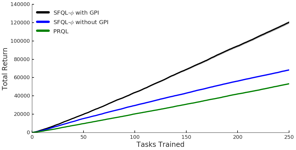
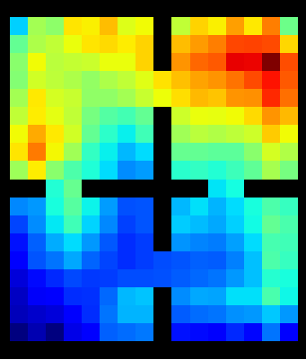
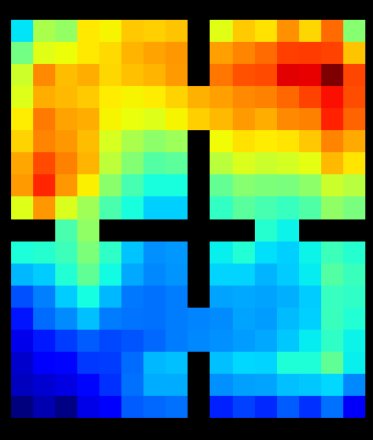
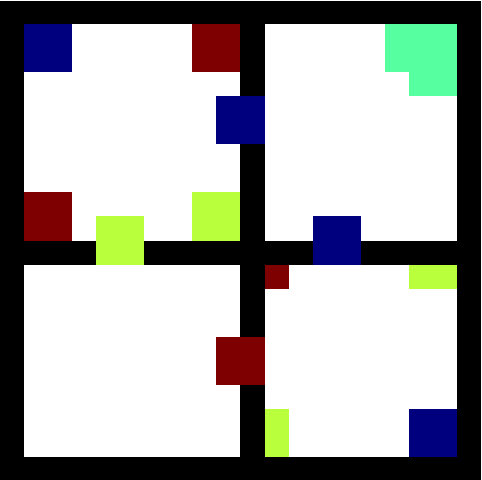
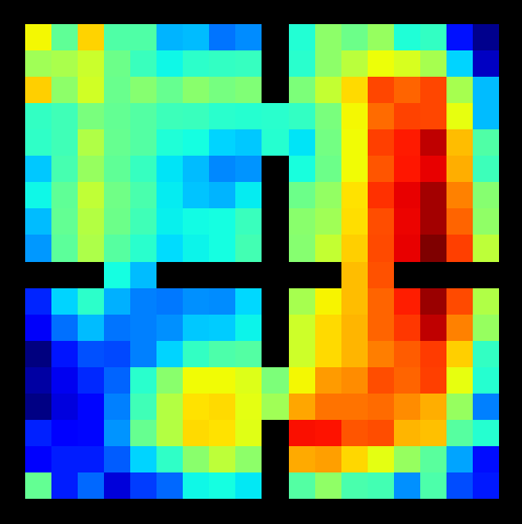
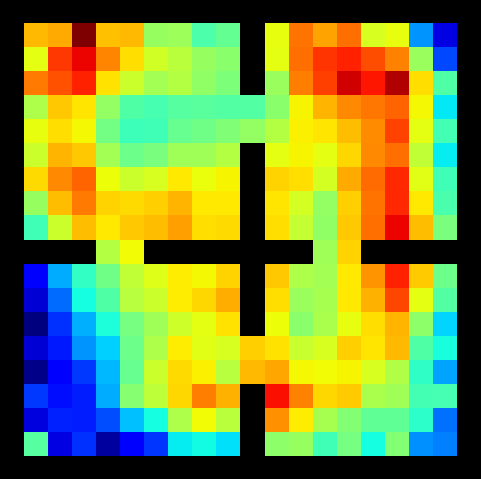
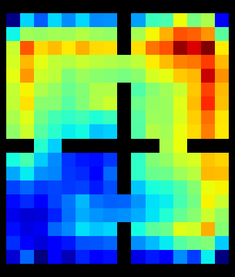
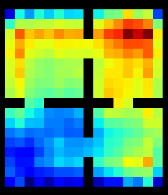
The results of our experiments are shown in Figure 4. It is interesting to note that even without GPI SFQL initially outperforms PRQL. This is probably the combined effect of the two factors discussed above: the decoupled representation of the value function plus the weak transfer promoted by $\tilde{\boldsymbol{\mathrm{\psi}}}^{\pi}$. Note though that, although these factors do give SFQL a head-start, eventually both algorithms reach the same performance level, as clear by the slope of the respective curves. In contrast, SFQL with GPI consistently outperforms the other two methods, which is evidence in favor of the hypothesis that GPI is indeed a crucial component of the proposed approach. Another evidence in this direction is given in Figure 5, which shows all the functions computed by the SFQL agent. Note how after only $200$ transitions into a new task SFQL already has a good approximation of the reward function, which, combined with the set of previously computed $\tilde{\boldsymbol{\mathrm{\psi}}}^{\pi_{i}}$, with $i<t$, provide a very informative value function even without the current $\tilde{\boldsymbol{\mathrm{\psi}}}^{\pi_{t}}$.

$\tilde{\boldsymbol{\mathrm{\phi}}}(s,a,s^{\prime})^{\top}\tilde{\boldsymbol{\mathrm{w}}}_{t}$	$\max\limits_{a,i<t}\tilde{\boldsymbol{\mathrm{\psi}}}_{i}(s,a)^{\top}\tilde{\boldsymbol{\mathrm{w}}}_{t}$	$\max\limits_{a,i\leq t}\tilde{\boldsymbol{\mathrm{\psi}}}_{i}(s,a)^{\top}\tilde{\boldsymbol{\mathrm{w}}}_{t}$

Figure 5: Functions computed by SFQL after $200$ transitions into three randomly selected tasks (all objects present).

C.2 Analyzing the robustness of SFs

As discussed in the previous section, part of the benefits provided by SFs come from the decoupled representation of the value function shown in (3), which depends crucially on a decomposition of the reward function $\tilde{\boldsymbol{\mathrm{\phi}}}(s,a,s^{\prime})^{\top}\boldsymbol{\mathrm{w}}\approx r(s,a,s^{\prime})$. In Section 5 we illustrated two ways in which such a decomposition can be obtained: by handcrafting $\tilde{\boldsymbol{\mathrm{\phi}}}$ based on prior knowledge about the environment or by learning it from data. When $\tilde{\boldsymbol{\mathrm{\phi}}}$ is learned it is obviously not reasonable to expect an exact decomposition of the reward function, but even when it is handcrafted the resulting reward model can be only an approximation (for example, the “object detector” used by the agents in the experiments with the four-room environment could be noisy). Regardless of the source of the imprecision, we do not want SFQL in particular, and more generally any method using SFs, to completely break with the addition of noise to $\tilde{\boldsymbol{\mathrm{\phi}}}$. In Section 5 we saw how an approximate $\tilde{\boldsymbol{\mathrm{\phi}}}$ can in fact lead to very good performance. In this section we provide a more systematic investigation of this matter by analyzing the performance of SFQL with $\tilde{\boldsymbol{\mathrm{\phi}}}$ corrupted in different ways.

Figure 6: Environment layout with additional objects. Spurious objects are represented as diamonds; numbers indicate the classes of the objects.

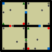
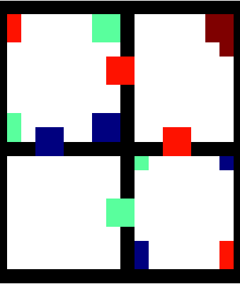
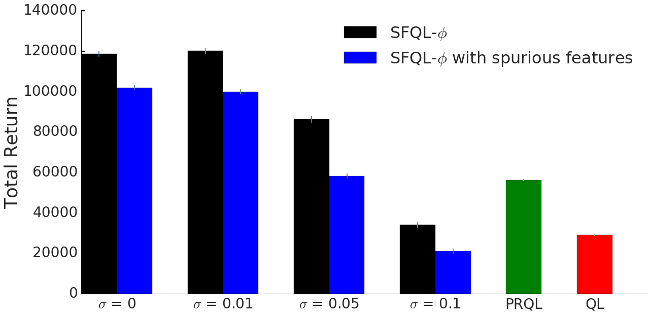
Our first experiment consisted in adding spurious features to $\boldsymbol{\mathrm{\phi}}$ that do not help in any way in the approximation of the reward function. This reflects the scenario where the agent’s set of predictions is a superset of the features needed to compute the reward (see in Section 6 the connection with Sutton et al.’s GVFs, 2011). In order to implement this, we added objects to our environment that always lead to zero reward—that is, even though the SFs $\tilde{\boldsymbol{\mathrm{\psi}}}^{\pi}$ learned by SFQL would predict the occurrence of these objects, such predictions would not help in the approximation of the reward function. Specifically, we added to our basic layout $15$ objects belonging to $6$ classes, as shown in Figure 6, which means that in this case SFQL used a $\tilde{\boldsymbol{\mathrm{\phi}}}\in\mathbb{R}^{10}$. In addition to adding spurious features, we also corrupted $\tilde{\boldsymbol{\mathrm{\phi}}}$ by adding to each of its components, in each step, a sample from a normal distribution with mean zero and different standard deviations $\sigma$.

The outcome of our experiment is shown in Figure 7. Overall, the results are as expected, with both spurious features and noise hurting the performance of SFQL. Interestingly, the two types of perturbations do not seem to interact very strongly, since their effects seem to combine in an additive way. More important, SFQL’s performance seems to degrade gracefully as a result of either intervention, which corroborate our previous experiments showing that the proposed approach is robust to approximation errors in $\tilde{\boldsymbol{\mathrm{\phi}}}$.

Figure 7: Analyzing SFQL’s robustness to distortions in $\tilde{\boldsymbol{\mathrm{\phi}}}$. PRQL’s and QL’s results are shown for reference. Results averaged over $30$ runs; standard errors are shown on top of each bar.

References

- Barto and Mahadevan [2003] Andrew G. Barto and Sridhar Mahadevan. Recent advances in hierarchical reinforcement learning. Discrete Event Dynamic Systems, 13(4):341–379, 2003.
- Baxter [2000] Jonathan Baxter. A model of inductive bias learning. Journal of Artificial Intelligence Research, 12:149–198, 2000.
- Bellman [1957] Richard E. Bellman. Dynamic Programming. Princeton University Press, 1957.
- Bernstein [1999] Daniel S. Bernstein. Reusing old policies to accelerate learning on new MDPs. Technical report, Amherst, MA, USA, 1999.
- Bertsekas and Tsitsiklis [1996] Dimitri P. Bertsekas and John N. Tsitsiklis. Neuro-Dynamic Programming. Athena Scientific, 1996.
- Caruana [1997] Rich Caruana. Multitask learning. Machine Learning, 28(1):41–75, 1997.
- Dayan [1993] Peter Dayan. Improving generalization for temporal difference learning: The successor representation. Neural Computation, 5(4):613–624, 1993.
- Fernández et al. [2010] Fernando Fernández, Javier García, and Manuela Veloso. Probabilistic policy reuse for inter-task transfer learning. Robotics and Autonomous Systems, 58(7):866–871, 2010.
- Hastie et al. [2002] Trevor Hastie, Robert Tibshirani, and Jerome Friedman. The Elements of Statistical Learning: Data Mining, Inference, and Prediction. Springer, 2002.
- Kulkarni et al. [2016] Tejas D. Kulkarni, Ardavan Saeedi, Simanta Gautam, and Samuel J Gershman. Deep successor reinforcement learning. arXiv preprint arXiv:1606.02396, 2016.
- Lazaric [2012] Alessandro Lazaric. Transfer in Reinforcement Learning: A Framework and a Survey. Reinforcement Learning: State-of-the-Art, pages 143–173, 2012.
- Lillicrap et al. [2015] Timothy P. Lillicrap, Jonathan J. Hunt, Alexander Pritzel, Nicolas Heess, Tom Erez, Yuval Tassa, David Silver, and Daan Wierstra. Continuous control with deep reinforcement learning. arXiv preprint arXiv:1509.02971, 2015.
- Littman et al. [2001] Michael L. Littman, Richard S. Sutton, and Satinder Singh. Predictive representations of state. In Advances in Neural Information Processing Systems (NIPS), pages 1555–1561, 2001.
- Mehta et al. [2008] Neville Mehta, Sriraam Natarajan, Prasad Tadepalli, and Alan Fern. Transfer in variable-reward hierarchical reinforcement learning. Machine Learning, 73(3), 2008.
- Mnih et al. [2015] Volodymyr Mnih, Koray Kavukcuoglu, David Silver, Andrei A. Rusu, Joel Veness, Marc G. Bellemare, Alex Graves, Martin Riedmiller, Andreas K. Fidjeland, Georg Ostrovski, Stig Petersen, Charles Beattie, Amir Sadik, Ioannis Antonoglou, Helen King, Dharshan Kumaran, Daan Wierstra, Shane Legg, and Demis Hassabis. Human-level control through deep reinforcement learning. Nature, 518(7540):529–533, 2015.
- Modayil et al. [2014] Joseph Modayil, Adam White, and Richard S. Sutton. Multi-timescale nexting in a reinforcement learning robot. Adaptive Behavior, 22(2):146–160, 2014.
- Natarajan and Tadepalli [2005] Sriraam Natarajan and Prasad Tadepalli. Dynamic preferences in multi-criteria reinforcement learning. In Proceedings of the International Conference on Machine Learning (ICML), pages 601–608, 2005.
- Ng and Russell [2000] Andrew Ng and Stuart Russell. Algorithms for inverse reinforcement learning. In Proceedings of the International Conference on Machine Learning (ICML), pages 663–670, 2000.
- Puterman [1994] Martin L. Puterman. Markov Decision Processes—Discrete Stochastic Dynamic Programming. John Wiley & Sons, Inc., 1994.
- Schaul et al. [2015] Tom Schaul, Daniel Horgan, Karol Gregor, and David Silver. Universal Value Function Approximators. In International Conference on Machine Learning (ICML), pages 1312–1320, 2015.
- Sutton and Barto [1998] Richard S. Sutton and Andrew G. Barto. Reinforcement Learning: An Introduction. MIT Press, 1998.
- Sutton et al. [1999] Richard S. Sutton, Doina Precup, and Satinder Singh. Between MDPs and semi-MDPs: a framework for temporal abstraction in reinforcement learning. Artificial Intelligence, 112:181–211, 1999.
- Sutton et al. [2011] Richard S. Sutton, Joseph Modayil, Michael Delp, Thomas Degris, Patrick M. Pilarski, Adam White, and Doina Precup. Horde: A scalable real-time architecture for learning knowledge from unsupervised sensorimotor interaction. In International Conference on Autonomous Agents and Multiagent Systems, pages 761–768, 2011.
- Szepesvári [2010] Csaba Szepesvári. Algorithms for Reinforcement Learning. Synthesis Lectures on Artificial Intelligence and Machine Learning. Morgan & Claypool Publishers, 2010.
- Taylor and Stone [2009] Matthew E. Taylor and Peter Stone. Transfer learning for reinforcement learning domains: A survey. Journal of Machine Learning Research, 10(1):1633–1685, 2009.
- Todorov et al. [2012] Emanuel Todorov, Tom Erez, and Yuval Tassa. MuJoCo: A physics engine for model-based control. In IEEE/RSJ International Conference on Intelligent Robots and Systems (IROS), pages 5026–5033, 2012.
- Watkins and Dayan [1992] Christopher Watkins and Peter Dayan. Q-learning. Machine Learning, 8:279–292, 1992.
- Yao et al. [2014] Hengshuai Yao, Csaba Szepesvári, Richard S Sutton, Joseph Modayil, and Shalabh Bhatnagar. Universal option models. In Advances in Neural Information Processing Systems (NIPS), pages 990–998. 2014.
- Zhang et al. [2016] Jingwei Zhang, Jost Tobias Springenberg, Joschka Boedecker, and Wolfram Burgard. Deep reinforcement learning with successor features for navigation across similar environments. CoRR, abs/1612.05533, 2016.
- Kingma and Ba [2014] Diederik Kingma and Jimmy Ba. Adam: A method for stochastic optimization. arXiv preprint arXiv:1412.6980, 2014.
- Strehl and Littman [2005] Alexander L. Strehl and Michael L. Littman. A theoretical analysis of model-based interval estimation. In Proceedings of the International Conference on Machine Learning (ICML), pages 857–864, 2005.