Rapid, Robust, and Reliable Blind Deconvolution via Nonconvex Optimization
Abstract
We study the question of reconstructing two signals and from their convolution . This problem, known as blind deconvolution, pervades many areas of science and technology, including astronomy, medical imaging, optics, and wireless communications. A key challenge of this intricate non-convex optimization problem is that it might exhibit many local minima. We present an efficient numerical algorithm that is guaranteed to recover the exact solution, when the number of measurements is (up to log-factors) slightly larger than the information-theoretical minimum, and under reasonable conditions on and . The proposed regularized gradient descent algorithm converges at a geometric rate and is provably robust in the presence of noise. To the best of our knowledge, our algorithm is the first blind deconvolution algorithm that is numerically efficient, robust against noise, and comes with rigorous recovery guarantees under certain subspace conditions. Moreover, numerical experiments do not only provide empirical verification of our theory, but they also demonstrate that our method yields excellent performance even in situations beyond our theoretical framework.
1 Introduction
Suppose we are given the convolution of two signals, . When, under which conditions, and how can we reconstruct and from the knowledge of if both and are unknown? This challenging problem, commonly referred to as blind deconvolution problem, arises in many areas of science and technology, including astronomy, medical imaging, optics, and communications engineering, see e.g. [14, 35, 9, 40, 5, 23, 10, 42]. Indeed, the quest for finding a fast and reliable algorithm for blind deconvolution has confounded researchers for many decades.
It is clear that without any additional assumptions, the blind deconvolution problem is ill-posed. One common and useful assumption is to stipulate that and belong to known subspaces [1, 25, 22, 27]. This assumption is reasonable in various applications, provides flexibility and at the same time lends itself to mathematical rigor. We also adopt this subspace assumption in our algorithmic framework (see Section 2 for details). But even with this assumption, blind deconvolution is a very difficult non-convex optimization problem that suffers from an overabundance of local minima, making its numerical solution rather challenging.
In this paper, we present a numerically efficient blind deconvolution algorithm that converges geometrically to the optimal solution. Our regularized gradient descent algorithm comes with rigorous mathematical convergence guarantees. The number of measurements required for the algorithm to succeed is only slightly larger than the information theoretic minimum. Moreover, our algorithm is also robust against noise. To the best of our knowledge, the proposed algorithm is the first blind deconvolution algorithm that is numerically efficient, robust against noise, and comes with rigorous recovery guarantees under certain subspace conditions.
1.1 State of the art
Since blind deconvolution problems are ubiquitous in science and engineering, it is not surprising that there is extensive literature on this topic. It is beyond the scope of this paper to review the existing literature; instead we briefly discuss those results that are closest to our approach. We gladly acknowledge that those papers that are closest to ours, namely [1, 7, 17, 34], are also the ones that greatly influenced our research in this project.
In the inspiring article [1], Ahmed, Recht, and Romberg develop a convex optimization framework for blind deconvolution. The formal setup of our blind deconvolution problem follows essentially their setting. Using the meanwhile well-known lifting trick, [1] transforms the blind deconvolution problem into the problem of recovering a rank-one matrix from an underdetermined system of linear equations. By replacing the rank condition by a nuclear norm condition, the computationally infeasible rank minimization problem turns into a convenient convex problem. The authors provide explicit conditions under which the resulting semidefinite program is guaranteed to have the same solution as the original problem. In fact, the number of required measurements is not too far from the theoretical minimum. The only drawback of this otherwise very appealing convex optimization approach is that the computational complexity of solving the semidefinite program is rather high for large-scale data and/or for applications where computation time is of the essence. Overcoming this drawback was one of the main motivations for our paper. While [1] does suggest a fast matrix-factorization based algorithm to solve the semidefinite program, the convergence of this algorithm to the optimal solution is not established in that paper. The theoretical number of measurements required in [1] for the semidefinite program to succeed is essentially comparable to that for our non-convex algorithm to succeed. The advantage of the proposed non-convex algorithm is of course that it is dramatically faster. Furthermore, numerical simulations indicate that the empirically observed number of measurements for our non-convex approach is actually smaller than for the convex approach.
The philosophy underlying the method presented in our paper is strongly motivated by the non-convex optimization algorithm for phase retrieval proposed in [7], see also [11, 3]. In the pioneering paper [7] the authors use a two-step approach: (i) Construct in a numerically efficient manner a good initial guess; (ii) Based on this initial guess, show that simple gradient descent will converge to the true solution. Our paper follows a similar two-step scheme. At first glance one would assume that many of the proof techniques from [7] should carry over to the blind deconvolution problem. Alas, we quickly found out that despite some general similarities between the two problems, phase retrieval and blind deconvolution are indeed surprisingly different. At the end, we mainly adopted some of the general “proof principles” from [7] (for instance we also have a notion of local regularity condition - although it deviates significantly from the one in [7]), but the actual proofs are quite different. For instance, in [7] and [11] convergence of the gradient descent algorithm is shown by directly proving that the distance between the true solution and the iterates decreases. The key conditions (a local regularity condition and a local smoothness condition) are tailored to this aim. For the blind deconvolution problem we needed to go a different route. We first show that the objective function decreases during the iterations and then use a certain local restricted isometry property to transfer this decrease to the iterates to establish convergence to the solution.
We also gladly acknowledge being influenced by the papers [17, 16] by Montanari and coauthors on matrix completion via non-convex methods. While the setup and analyzed problems are quite different from ours, their approach informed our strategy in various ways. In [17, 16], the authors propose an algorithm which comprises a two-step procedure. First, an initial guess is computed via a spectral method, and then a nonconvex problem is formulated and solved via an iterative method. The authors prove convergence to a low-rank solution, but do not establish a rate of convergence. As mentioned before, we also employ a two-step strategy. Moreover, our approach to prove stability of the proposed algorithm draws from ideas in [16].
We also benefitted tremendously from [34]. In that paper, Sun and Luo devise a non-convex algorithm for low-rank matrix completion and provide theoretical guarantees for convergence to the correct solution. We got the idea of adding a penalty term to the objective function from [34] (as well as from [17]). Indeed, the particular structure of our penalty term closely resembles that in [34]. In addition, the introduction of the various neighborhood regions around the true solution, that are used to eventually characterize a “basin of attraction”, stems from [34]. These correspondences may not be too surprising, given the connections between low-rank matrix completion and blind deconvolution. Yet, like also discussed in the previous paragraph, despite some obvious similarities between the two problems, it turned out that many steps and tools in our proofs differ significantly from those in [34]. Also this should not come as a surprise, since the measurement matrices and setup differ significantly111Anyone who has experience in the proofs behind compressive sensing and matrix completion is well aware of the substantial challenges one can already face by “simply” changing the sensing matrix from, say, a Gaussian random matrix to one with less randomness.. Moreover, unlike [34], our paper also provides robustness guarantees for the case of noisy data. Indeed, it seems plausible that some of our techniques to establish robustness against noise are applicable to the analysis of various recent matrix completion algorithms, such as e.g. [34].
We briefly discuss other interesting papers that are to some extent related to our work. [22] proposes a projected gradient descent algorithm based on matrix factorizations and provide a convergence analysis to recover sparse signals from subsampled convolution. However, this projection step can be hard to implement, which does impact the efficiency and practical use of this method. As suggested in [22], one can avoid this expensive projection step by resorting to a heuristic approximate projection, but then the global convergence is not fully guaranteed. On the other hand, the papers [25, 24] consider identifiability issue of blind deconvolution problem with both and in random linear subspaces and achieve nearly optimal result of sampling complexity in terms of information theoretic limits. Very recently, [15] improved the result from [25, 24] by using techniques from algebraic geometry.
The past few years have also witnessed an increasing number of excellent works other than blind deconvolution but related to nonconvex optimization [32, 41, 31, 3, 21]. The paper [37] analyzes the problem of recovering a low-rank positive semidefinite matrix from linear measurements via a gradient descent algorithm. The authors assume that the measurement matrix fulfills the standard and convenient restricted isometry property, a condition that is not suitable for the blind deconvolution problem (besides the fact that the positive semidefinite assumption is not satisfied in our setting). In [12], Chen and Wainwright study various the solution of low-rank estimation problems by projected gradient descent. The very recent paper [43] investigates matrix completion for rectangular matrices. By “lifting”, they convert the unknown matrix into a positive semidefinite one and apply matrix factorization combined with gradient descent to reconstruct the unknown entries of the matrix. [4] considers an interesting blind calibration problem with a special type of measurement matrix via nonconvex optimization. Besides some general similarities, there is little overlap of the aforementioned papers with our framework. Finally, a convex optimization approach to blind deconvolution and self-calibration that extends the work of [1] can be found in [27], while [26] also covers the joint blind deconvolution-blind demixing problem.
1.2 Organization of our paper
This paper is organized as follows. We introduce some notation used throughout the paper in the remainder of this section. The model setup and problem formulation are presented in Section 2. Section 3 describes the proposed algorithm and our main theoretical result establishing the convergence of our algorithm. Numerical simulations can be found in Section 4. Section 5 is devoted to the proof of the main theorem. Since the proof is quite involved, we have split this section into several subsections. Some auxiliary results are collected in the Appendix.
1.3 Notation
We introduce notation which will be used throughout the paper. Matrices and vectors are denoted in boldface such as and . The individual entries of a matrix or a vector are denoted in normal font such as or For any matrix , denotes its nuclear norm, i.e., the sum of its singular values; denotes its operator norm, i.e., the largest singular value, and denotes its the Frobenius norm, i.e., . For any vector , denotes its Euclidean norm. For both matrices and vectors, and stand for the transpose of and respectively while and denote their complex conjugate transpose. We equip the matrix space with the inner product defined as A special case is the inner product of two vectors, i.e., For a given vector , represents the diagonal matrix whose diagonal entries are given by the vector . For any , denote as is an absolute constant and is a constant which depends linearly on , but on no other parameters.
2 Problem setup
We consider the blind deconvolution model
| (2.1) |
where is given, but and are unknown. Here “” denotes circular convolution222As usual, ordinary convolution can be well approximated by circulant convolution, as long as the function decays sufficiently fast [30].. We will usually consider as the “blurring function” and as the signal of interest. It is clear that without any further assumption it is impossible to recover and from . We want to impose conditions on and that are realistic, flexible, and not tied to one particular application (such as, say, image deblurring). At the same time, these conditions should be concrete enough to lend themselves to meaningful mathematical analysis.
A natural setup that fits these demands is to assume that and belong to known linear subspaces. Concerning the blurring function, it is reasonable in many applications to assume that is either compactly supported or that decays sufficiently fast so that it can be well approximated by a compactly supported function. Therefore, we assume that satisfies
| (2.2) |
where , i.e., only the first entries of are nonzero and for all . Concerning the signal of interest, we assume that belongs to a linear subspace spanned by the columns of a known matrix , i.e., for some matrix of size . Here we use instead of for the simplicity of notation later. For theoretical purposes we assume that is a Gaussian random matrix. Numerical simulations suggest that this assumption is clearly not necessary. For example, we observed excellent performance of the proposed algorithm also in cases when represents a wavelet subspace (appropriate for images) or when is a Hadamard-type matrix (appropriate for communications). We hope to address these other, more realistic, choices for in our future research. Finally, we assume that as the additive white complex Gaussian noise where and and are the true blurring function and the true signal of interest, respectively. In that way actually serves as a measure of SNR (signal to noise ratio).
For our theoretical analysis as well as for numerical purposes, it is much more convenient to express (2.1) in the Fourier domain, see also [1]. To that end, let be the unitary Discrete Fourier Transform (DFT) matrix and let the matrix be given by the first columns of (then ). By applying the scaled DFT matrix to both sides of (2.1) we get
| (2.3) |
which follows from the property of circular convolution and Discrete Fourier Transform. Here, where denotes pointwise product. By definition of in (2.2), we have
Therefore, (2.3) becomes,
| (2.4) |
where (we use instead of simply because it gives rise to a more convenient notation later, see e.g. (2.8)).
Note that if is a Gaussian matrix, then so is . Furthermore, is again a complex Gaussian random vector. Hence by replacing in (2.4) by , we arrive with a slight abuse of notation at
| (2.5) |
For the remainder of the paper, instead of considering the original blind deconvolution problem (2.1), we focus on its mathematically equivalent version (2.5), where , , , and . As mentioned before, and are the ground truth. Our goal is to recover and when , and are given. It is clear that if is a solution to the blind deconvolution problem. then so is for any . Thus, all we can hope for in the absence of any further information, is to recover a solution from the equivalence class . Hence, we can as well assume that .
As already mentioned, we choose to be the “low-frequency” discrete Fourier matrix, i.e., the first columns of an unitary DFT (Discrete Fourier Transform) matrix. Moreover, we choose to be an complex Gaussian random matrix, i.e.,
where “” is the imaginary unit.
We define the matrix-valued linear operator via
| (2.6) |
where denotes the -th column of and is the -th column of Immediately, we have , and for all . This is essentially a smart and popular trick called “lifting” [8, 1, 27], which is able to convert a class of nonlinear models into linear models at the costs of increasing the dimension of the solution space.
It seems natural and tempting to recover obeying (2.5) by solving the following optimization problem
| (2.7) |
where
| (2.8) |
We also let
| (2.9) |
which is a special case of when Furthermore, we define , an important quantity throughout our discussion, via
| (2.10) |
When there is no danger of ambiguity, we will often denote simply by . But let us remember that is always a function of and measures the relative approximation error of .
Obviously, minimizing (2.8) becomes a nonlinear least square problem, i.e., one wants to find a pair of vectors or a rank-1 matrix which fits the measurement equation in (2.8) best. Solving (2.7) is a challenging optimization problem since it is highly nonconvex and most of the available algorithms, such as alternating minimization and gradient descent, may suffer from getting easily trapped in some local minima. Another possibility is to consider a convex relaxation of (2.7) at the cost of having to solve an expensive semidefinite program. In the next section we will describe how to avoid this dilemma and design an efficient gradient descent algorithm that, under reasonable conditions, will always converge to the true solution.
3 Algorithm and main result
In this section we introduce our algorithm as well as our main theorems which establish convergence of the proposed algorithm to the true solution. As mentioned above, in a nutshell our algorithm consists of two parts: First we use a carefully chosen initial guess, and second we use a variation of gradient descent, starting at the initial guess to converge to the true solution. One of the most critical aspects is of course that we must avoid getting stuck in local minimum or saddle point. Hence, we need to ensure that our iterates are inside some properly chosen basin of attraction of the true solution. The appropriate characterization of such a basin of attraction requires some diligence, a task that will occupy us in the next subsection. We will then proceed to introducing our algorithm and analyzing its convergence.
3.1 Building a basin of attraction
The road toward designing a proper basin of attraction is basically paved by three observations, described below. These observations prompt us to introduce three neighborhoods (inspired by [17, 34]), whose intersection will form the desired basin of attraction of the solution.
Observation 1 - Nonuniqueness of the solution: As pointed out earlier, if is a solution to (2.5), then so is for any . Thus, without any prior information about and/or , it is clear that we can only recover the true solution up to such an unknown constant . Fortunately, this suffices for most applications. From the viewpoint of numerical stability however, we do want to avoid, while remains bounded, that and (or vice versa). To that end we introduce the following neighborhood:
| (3.1) |
(Recall that .)
Observation 2 - Incoherence: Our numerical simulations indicate that the number of measurements required for solving the blind deconvolution problem with the proposed algorithm does depend (among others) on how much is correlated with the rows of the matrix — the smaller the correlation the better. A similar effect has been observed in blind deconvolution via convex programming [1, 26]. We quantify this property by defining the incoherence between the rows of and via
| (3.2) |
It is easy to see that and both lower and upper bounds are tight; i.e., if is parallel to one of and if is a 1-sparse vector of length . Note that in our setup, we assume that is a random matrix and is fixed, thus with high probability, is already sufficiently incoherent with the rows of and thus we only need to worry about the incoherence between and .
It should not come as a complete surprise that the incoherence between and the rows of is important. The reader may recall that in matrix completion [6, 28] the left and right singular vectors of the solution cannot be “too aligned” with those of the measurement matrices. A similar philosophy seems to apply here. Being able to control the incoherence of the solution is instrumental in deriving rigorous convergence guarantees of our algorithm. For that reason, we introduce the neighborhood
| (3.3) |
where .
Observation 3 - Initial guess: It is clear that due to the non-convexity of the objective function, we need a carefully chosen initial guess. We quantify the distance to the true solution via the following neighborhood
| (3.4) |
where is a predetermined parameter in .
It is evident that the true solution . Note that implies and . Therefore, for any element its incoherence can be well controlled by
3.2 Objective function and key ideas of the algorithm
Our approach consists of two parts: We first construct an initial guess that is inside the “basin of attraction” . We then apply a carefully regularized gradient descent algorithm that will ensure that all the iterates remain inside .
Due to the difficulties of directly projecting onto (the neigbourhood is easier to manage) we add instead a regularizer to the objective function to enforce that the iterates remain inside . While the idea of adding a penalty function to control incoherence is proposed in different forms to solve matrix completion problems, see e.g., [33, 20], our version is mainly inspired by [34, 17].
Hence, we aim to minimize the following regularized objective function to solve the blind deconvolution problem:
| (3.5) |
where is defined in (2.8) and , the penalty function, is of the form
| (3.6) |
where and . Here we assume and .
The idea behind this, at first glance complicated, penalty function is quite simple. The first two terms in (3.6) enforce the projection of onto while the last term is related to ; it will be shown later that any gives if . Since is a truncated quadratic function, it is obvious that and is a continuously differentiable function. Those two properties play a crucial role in proving geometric convergence of our algorithm presented later.
Another important issue concerns the selection of parameters. We have three unknown parameters in , i.e., , , and . Here, can be obtained via Algorithm 1 and is guaranteed by Theorem 3.1; because and concentrates around . In practice, which is the inverse of the SNR, can often be well estimated. Regarding , we require in order to make sure that . It will depend on the specific application how well one can estimate . For instance, in wireless communications, a very common channel model for is to assume a Rayleigh fading model [36], i.e., . In that case it is easy to see that
3.3 Wirtinger derivative of the objective function and algorithm
Since we are dealing with complex variables, instead of using regular derivatives it is more convenient to utilize Wirtinger derivatives 333For any complex function where and , the Wirtinger derivatives are defined as and Two important examples used here are and . , which has become increasingly popular since [7, 3]. Note that is a real-valued function and hence we only need to consider the derivative of with respect to and and the corresponding updates of and because a simple relation holds, i.e.,
In particular, we denote and .
We also introduce the adjoint operator of , given by
| (3.7) |
Both and can now be expressed as
where each component yields
| (3.8) | |||||
| (3.9) | |||||
| (3.10) | |||||
| (3.11) |
Our algorithm consists of two steps: initialization and gradient descent with constant stepsize. The initialization is achieved via a spectral method followed by projection. The idea behind spectral method is that
and hence one can hope that the leading singular value and vectors of can be a good approximation of and respectively. The projection step ensures , which the spectral method alone might not guarantee. We will address the implementation and computational complexity issue in Section 4.
3.4 Main results
Our main finding is that with a diligently chosen initial guess , simply running gradient descent to minimize the regularized non-convex objective function will not only guarantee linear convergence of the sequence to the global minimum in the noiseless case, but also provide robust recovery in the presence of noise. The results are summarized in the following two theorems.
Theorem 3.1.
The initialization obtained via Algorithm 1 satisfies
| (3.12) |
and
| (3.13) |
holds with probability at least if the number of measurements satisfies
| (3.14) |
Here is any predetermined constant in , and is a constant only linearly depending on with .
The proof of Theorem 3.1 is given in Section 5.5. While the initial guess is carefully chosen, it is in general not of sufficient accuracy to already be used as good approximation to the true solution. The following theorem establishes that as long as the initial guess lies inside the basin of attraction of the true solution, regularized gradient descent will indeed converge to this solution (or to a solution nearby in case of noisy data).
Theorem 3.2.
Consider the model in (2.5) with the ground truth , and the noise . Assume that the initialization belongs to and that
Algorithm 2 will create a sequence which converges geometrically to in the sense that with probability at least , there holds
| (3.15) |
and
| (3.16) |
where , , is the fixed stepsize and is the angle between and . Here
| (3.17) |
holds with probability
Remarks:
- 1.
-
2.
The minimum number of measurements required for our method to succeed is roughly comparable to that of the convex approach proposed in [1] (up to log-factors). Thus there is no price to be paid for trading a slow, convex-optimization based approach with a fast non-convex based approach. Indeed, numerical experiments indicate that the non-convex approach even requires a smaller number of measurements compared to the convex approach, see Section 4.
-
3.
The convergence rate of our algorithm is completely determined by . Here, the regularity constant is specified in (5.7) and where . The attentive reader may have noted that depends essentially linearly on , which actually reflects a tradeoff between sampling complexity (or statistical estimation quality) and computation time. Note that if gets larger, the number of constraints is also increasing and hence leads to a larger . However, this issue can be solved by choosing parameters smartly. Theorem 3.2 tells us that should be roughly between and . Therefore, by choosing and , is optimized and
which is shown in details in Section 5.4.
- 4.
-
5.
The matrix , as a sum of rank-1 random matrices, has nice concentration of measure properties under the assumption of Theorem 3.2. Asymptotically, converges to with rate , which will be justified in Lemma 5.20 of Section 5.5 (see also [3]). Note that
(3.19) If one lets , then will converge almost surely to under the Law of Large Numbers and the cross term will converge to . In other words, asymptotically,
for all fixed . This implies that if the number of measurements is large, then behaves “almost like” , the noiseless version of . This provides the key insight into analyzing the robustness of our algorithm, which is reflected in the so-called “Robustness Condition” in (5.2). Moreover, the asymptotic property of is also seen in our main result (3.18). Suppose is becoming larger and larger, the effect of noise diminishes and heuristically, we might just rewrite our result as , which is consistent with the result without noise.
4 Numerical simulations
We present empirical evaluation of our proposed gradient descent algorithm (Algorithm 2) using simulated data as well as examples from blind deconvolution problems appearing in communications and in image processing.
4.1 Number of measurements vs size of signals
We first investigate how many measurements are necessary in order for an algorithm to reliably recover two signals from their convolution. We compare Algorithm 2, a gradient descent algorithm for the sum of the loss function and the regularization term , with the gradient descent algorithm only applied to and the nuclear norm minimization proposed in [1]. These three tested algorithms are abbreviated as regGrad, Grad and NNM respectively. To make fair comparisons, both regGrad and Grad are initialized with the normalized leading singular vectors of , which are computed by running the power method for iterations. Though we do not further compute the projection of for regGrad as stated in the third step of Algorithm 1, we emphasize that the projection can be computed efficiently as it is a linear programming on -dimensional vectors. A careful reader may notice that in addition to the computational cost for the loss function , regGrad also requires to evaluate and its gradient in each iteration. When consists of the first columns of a unitary DFT matrix, we can evaluate and the gradient of using FFT. Thus the additional per iteration computational cost for the regularization term is only flops. The stepsizes in both regGrad and Grad are selected adaptively in each iteration via backtracking. As suggested by the theory, the choices for and in regGrad are and .
We conduct tests on random Gaussian signals and with . The matrix is the first columns of a unitary DFT matrix, while is either a Gaussian random matrix or a partial Hadamard matrix with randomly selected columns and then multiplied by a random sign matrix from the left. When is a Gaussian random matrix, takes equal spaced values from to . When is a partial Hadamard matrix, we only test with being integers. For each given triple , fifty random tests are conducted. We consider an algorithm to have successfully recovered if it returns a matrix which satisfies
We present the probability of successful recovery plotted against the number of measurements in Figure 1.
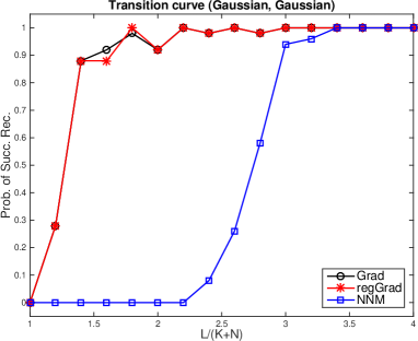
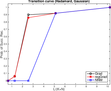
It can be observed that regGrad and Grad have similar performance, and both of them require a significantly smaller number of measurements than NNM to achieve successful recovery of high probability.
4.2 Number of measurements vs incoherence
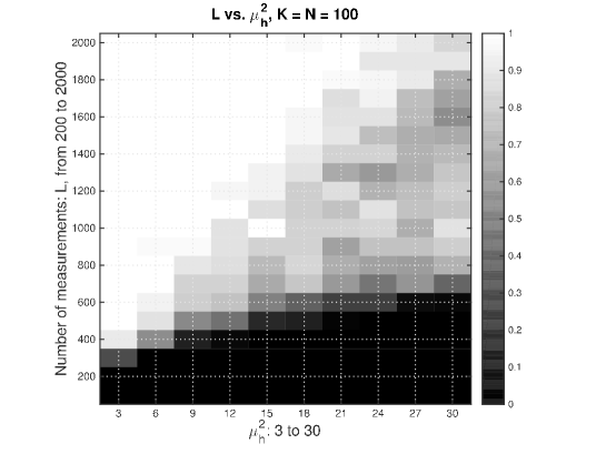
Theorem 3.2 indicates that the number of measurements required for Algorithm 2 to achieve successful recovery scales linearly with . We conduct numerical experiments to investigate the dependence of on empirically. The tests are conducted with taking on values . For each fixed , we choose to be a vector whose first entries are and the others are so that its incoherence is equal to when is low frequency Fourier matrix. Then the tests are repeated for random Gaussian matrices and random Gaussian vectors . The empirical probability of successful recovery on the plane is presented in Figure 2, which suggests that does scale linearly with .
4.3 A comparison when is large
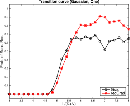
While regGrad and Grad have similar performances in the simulation when is a random Gaussian signal (see Figure 1), we investigate their performances on a fixed with a large incoherence. The tests are conducted for , being a random Gaussian signal, being a random Gaussian matrix, and being a low frequency Fourier matrix. The signal with is formed in the same way as in Section 4.2; that is, the first entries of are one and the other entries are zero. The number of measurements varies from to . For each , random tests are conducted. Figure 3 shows the probability of successful recovery for regGrad and Grad. It can be observed that the successful recovery probability of regGrad is at least larger than that of Grad when .
4.4 Robustness to additive noise
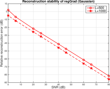
We explore the robustness of Algorithm 2 when the measurements are contaminated by additive noise. The tests are conducted with , when is a random Gaussian matrix, and when is a partial Hadamard matrix. Tests with additive noise have the measurement vector corrupted by the vector
where is standard Gaussian random vector, and takes nine different values from to . For each , fifty random tests are conducted. The average reconstruction error in dB plotted against the signal to noise ratio (SNR) is presented in Fig. 4. First the plots clearly show the desirable linear scaling between the noise levels and the relative reconstruction errors. Moreover, as desired, the relative reconstruction error decreases linearly on a - scale as the number of measurements increases.

4.5 An example from communications
In order to demonstrate the effectiveness of Algorithm 2 for real world applications, we first test the algorithm on a blind deconvolution problem arising in communications. Indeed, blind deconvolution problems and their efficient numerical solution are expected to play an increasingly important role in connection with the emerging Internet-of-Things [42]. Assume we want to transmit a signal from one place to another over a so-called time-invariant multi-path communication channel, but the receiver has no information about the channel, except its delay spread (i.e., the support of the impulse response). In many communication settings it is reasonable to assume that the receiver has information about the signal encoding matrix—in other words, we know the subspace to which belongs to. Translating this communications jargon into mathematical terminology, this simply means that we are dealing with a blind deconvolution problem of the form (2.5).
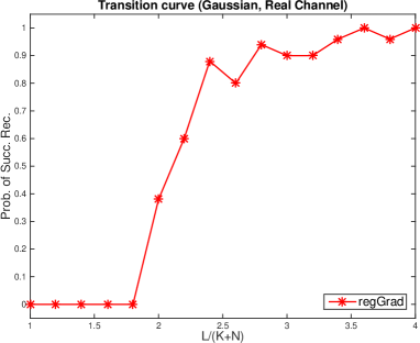
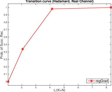
These encoding matrices (or so-called spreading matrices) are often chosen to have a convenient structure that lends itself to fast computations and minimal memory requirements. One such choice is to let , where the matrix consists of (randomly or not randomly) chosen columns of an Hadamard matrix, premultiplied with an diagonal random sign matrix . Instead of a partial Hadamard matrix we could also use a partial Fourier matrix; the resulting setup would then closely resemble an OFDM transmission format, which is part of every modern wireless communication scheme. For the signal we choose a so-called QPSK scheme, i.e., each entry of takes a value from with equal probability. The actual transmitted signal is then . For the channel (the blurring function) we choose a real-world channel, courtesy of Intel Corporation. Here, represents the impulse response of a multipath time-invariant channel, it consists of 123 time samples, hence . Otherwise, the setup follows closely that in Sec. 4.1. For comparison we also include the case when is a random Gaussian matrix.
The plots of successful recovery probability are presented in Figure 5, which shows that Algorithm 2 can successfully recover the real channel with high probability if when is a random Gaussian matrix and if when is a partial Hadamard matrix. Thus our theory seems a bit pessimistic. It is gratifying to see that very little additional measurements are required compared to the number of unknowns in order to recover the transmitted signal.


4.6 An example from image processing
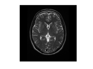
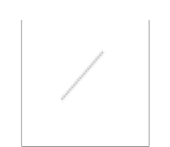
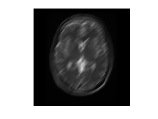
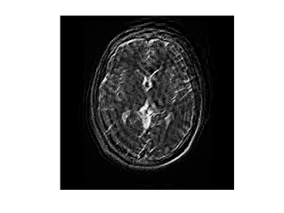
Next, we test Algorithm 2 on an image deblurring problem, inspired by [1]. The observed image (Figure 6c) is a convolution of a MRI image (Figure 6a) with a motion blurring kernel (Figure 6b). Since the MRI image is approximately sparse in the Haar wavelet basis, we can assume it belongs to a low dimensional subspace; that is, , where with denotes the MRI image reshaped into a vector, represents the wavelet subspace and is the vector of wavelet coefficients. The blurring kernel is supported on a low frequency region. Therefore , where is a reshaped D low frequency Fourier matrix and is a short vector.
Figure 6d shows the initial guess for Algorithm 2 in the image domain, which is obtained by running the power method for fifty iterations. While this initial guess is clearly not a good approximation to the true solution, it suffices as a starting point for gradient descent. In the first experiment, we take to be the wavelet subspace corresponding to the largest Haar wavelet coefficients of the original MRI image, and we also assume the locations of the nonzero entries of the kernel are known. Figure 6e shows the reconstructed image in this ideal setting. It can be observed that the recovered image is visually indistinguishable from the ground truth MRI image. In the second experiment, we test a more realistic setting, where both the support of the MRI image is the wavelet domain and the support of the kernel are not known. We take the Haar wavelet transform of the blurred image (Figure 6c) and select to be the wavelet subspace corresponding to the largest wavelet coefficients. We do not assume the exact support of the kernel is known, but assume that its support is contained in a small box region. The reconstructed image in this setting is shown in Figure 6f. Despite not knowing the subspaces exactly, Algorithm 2 is still able to return a reasonable reconstruction.
Yet, this second experiment also demonstrates that there is clearly room for improvement in the case when the subspaces are unknown. One natural idea to improve upon the result depicted in Figure 6f is to include an additional total-variation penalty in the reconstruction algorithm. We leave this line of work for future research.
5 Proof of the main theorem
This section is devoted to the proof of Theorems 3.1 and 3.2. Since proving Theorem 3.2 is a bit more involved, we briefly describe the architecture of its proof. In Subsection 5.1 we state four key conditions: The Local Regularity Condition will allow us to show that the objective function decreases; the Local Restricted Isometry Property enables us to transfer the decrease in the objective function to a decrease of the error between the iterates and the true solution; the Local Smoothness Condition yields the actual rate of convergence, and finally, the Robustness Condition establishes robustness of the proposed algorithm against additive noise. Armed with these conditions, we will show how the three regions defined in Section 3 characterize the convergence neighborhood of the solution, i.e., if the initial guess is inside this neighborhood, the sequence generated via gradient descent will always stay inside this neighborhood as well. In Subsections 5.2–5.5 we justify the aforementioned four conditions, show that they are valid under the assumptions stated in Theorem 3.2, and conclude with a proof of Theorem 3.1.
5.1 Four key conditions and the proof of Theorem 3.2
Condition 5.1 (Local RIP condition).
The following local Restricted Isometry Property (RIP) for holds uniformly for all
| (5.1) |
Condition 5.1 states that almost preserves the -distance between over a “local” region around the ground truth . The proof of Condition 5.1 is given in Lemma 5.14.
Condition 5.2 (Robustness condition).
For the noise , with high probability there holds,
| (5.2) |
if .
This condition follows directly from (3.17). It is quite essential when we analyze the behavior of Algorithm 2 under Gaussian noise. With those two conditions above in hand, the lower and upper bounds of are well approximated over by two quadratic functions of , where is defined in (2.10). A similar approach towards noisy matrix completion problem can be found in [16]. For any , applying Condition 5.1 to (3.19) leads to
| (5.3) |
and similarly
| (5.4) |
where
because and is a pair of dual norm and . Moreover, with the Condition 5.2, (5.3) and (5.4) yield the followings:
| (5.5) |
and
| (5.6) |
The third condition is about the regularity condition of , which is the key to establishing linear convergence later. The proof will be given in Lemma 5.18.
Condition 5.3 (Local regularity condition).
Let be as defined in (3.5) and . Then there exists a regularity constant such that
| (5.7) |
for all where with . In particular, in the noiseless case, i.e., , we have
Besides the three regions defined in (3.1) to (3.3), we define another region via
| (5.8) |
for proof technical purposes. is actually the sublevel set of the nonconvex function .
Finally we introduce the last condition called Local smoothness condition and its corresponding quantity which characterizes the choice of stepsize and the rate of linear convergence.
Condition 5.4 (Local smoothness condition).
Denote . There exists a constant such that
| (5.9) |
for all , i.e., the whole segment connecting and , which is parametrized by , belongs to the nonconvex set
The upper bound of , which scales with , will be given in Section 5.4. We will show later in Lemma 5.8 that the stepsize is chosen to be smaller than Hence
Proof: .
If , by the definition of in (3.6), at least one component in exceeds . We have
where and
This implies and hence .
This lemma implies that the intersection of and the boundary of is empty. One might believe this suggests that . This may not be true. A more reasonable interpretation is that consists of several disconnected regions due to the non-convexity of , and one or several of them are contained in .
Lemma 5.6.
Denote and . Let . If and for all , we have .
Proof: .
Let us prove the claim by contradiction. If , since , there exists for some , such that . However, since , by Lemma 5.5, we have . This leads to a contradiction.
Remark 5.7.
Lemma 5.6 tells us that if one line segment is completely inside with one end point in , then this whole line segment lies in
Lemma 5.8.
Let the stepsize , and be the constant defined in (5.9). Then, as long as , we have and
| (5.10) |
Proof: .
It suffices to prove (5.10). If , then , which implies (5.10) directly. So we only consider the case when . Define the function
Then
since is a real-valued function with complex variables (See (6.1) for details). By the definition of derivatives, we know there exists , such that for all . Now we will first prove that for all by contradiction. Assume there exists some such that . Then there exists , such that and for all , since is a continuous function. This implies
since for By Lemma 5.6 and the assumption , we have
Then, by using the modified descent lemma (Lemma 6.1),
where the final inequality is due to , and . This contradicts .
Therefore, there holds for all . Similarly, we can prove
which implies . Again, by using Lemma 6.1 we can prove
where the final inequality is due to .
We conclude this subsection by proving Theorem 3.2 under the Local regularity condition, the Local RIP condition, the Robustness condition, and the Local smoothness condition. The next subsections are devoted to justifying these conditions and showing that they hold under the assumptions of Theorem 3.2.
Proof: .
[of Theorem 3.2] Suppose that the initial guess , we have . This holds, because
where , and Therefore for all and Since , (5.5) combined with imply that
and hence Denote Combining Lemma 5.8 by choosing with Condition 5.3, we have
with , and for all Obviously, the inequality above implies
and by monotonicity of , there holds
Therefore, by induction, we have
where and hence Now we can conclude that converges to geometrically. Note that over ,
where , is defined in (2.9) and . There holds
and equivalently,
Solving the inequality above for , we have
| (5.11) | |||||
Let , By (5.11) and triangle inequality, we immediately conclude that
Now we derive the upper bound for and Due to symmetry, it suffices to consider . The bound follows from standard linear algebra arguments:
where the second equality uses
5.2 Supporting lemmata
This subsection introduces several lemmata, especially Lemma 5.9, 5.12 and 5.13, which are central for justifying Conditions 5.1 and 5.3. After that, we will prove the Local RIP Condition in Lemma 5.14 based on those three lemmata. We start with defining a linear space , which contains , via
| (5.12) |
Its orthogonal complement is given by
Denote to be the projection operator from onto .
For any and , there are unique orthogonal decompositions
| (5.13) |
where and . More precisely, and We thereby have the following matrix orthogonal decomposition
| (5.14) |
where the first three components are in while .
Lemma 5.9.
Recall that . If , we have the following useful bounds
and
Moreover, if and , we have .
Remark 5.10.
This lemma is actually a simple version of singular value/vector perturbation. It says that if is of , then the individual vectors are also close to , with the error of order
Proof: .
The equality (5.13) implies that , so there holds . Since , by (5.14), we have
| (5.15) |
This implies that
On the other hand,
The above two inequalities imply that , and similarly we have . The equality (5.15) implies that and hence . Moreover, (5.15) also implies
which yields .
If and , there holds . Then
where .
In the following, we introduce and prove a series of local and global properties of :
Lemma 5.12 (Corollary 2 in [1]).
Let be the operator defined in (2.6), then on an event with probability at least , restricted on is well-conditioned, i.e.,
where is the projection operator from onto , provided .
Now we introduce a property of when restricted on rank-one matrices.
Lemma 5.13.
On an event with probability at least , we have
uniformly for any and , provided .
Proof: .
Due to the homogeneity, without loss of generality we can assume . Define
It suffices to prove that uniformly for all with high probability, where is the unit sphere in For fixed , notice that
is the sum of subexponential variables with expectation . For any generalized variable satisfies
| (5.17) |
where are i.i.d. random variables and . Here we set , and . Therefore,
and we have
Applying (5.17) and setting
there holds
That is, with probability at least . We define and as -nets of and , respectively. Then, and follow from the covering numbers of the sphere (Lemma 5.2 in [39]).
By taking the union bounds over we have holds uniformly for all with probability at least
Our goal is to show that uniformly for all with the same probability. For any , we can find its closest satisfying and . By Lemma 5.11, with probability at least , we have . Then straightforward calculation gives
where the first inequality is due to for any , and the second inequality is due to for any . Similarly,
Therefore, if , there holds
Therefore, if with reasonably large and , we have and uniformly for all with probability at least .
Finally, we introduce a local RIP property of conditioned on the event , where and are defined in Lemma 5.12 and Lemma 5.13
Lemma 5.14.
Over with and , the following RIP type of property holds for :
provided for some numerical constant and conditioned on
Proof: .
Let , and
where
| (5.18) |
By Lemma 5.9, we have and hence
Since , by Lemma 5.12, we have
| (5.19) |
By Lemma 5.13, we have
| (5.20) |
By Lemma 5.9, we have , , , and . By substituting all those estimations into (5.20), it ends up with
| (5.21) |
where is a numerical constant and . Combining (5.21) and (5.19) together with sufficiently large, numerical computation gives
for all given .
5.3 Local regularity
In this subsection, we will prove Condition 5.3. Throughout this section, we assume and holds where and are mentioned in Lemma 5.12 and Lemma 5.13. For all , consider and defined in (5.13) and let
where
with . The particular form of serves primarily for proving the local regularity condition of , which will be evident in Lemma 5.17.
The following lemma gives bounds of and .
Lemma 5.15.
For all with , there holds , , and . Moreover, if we assume additionally, we have .
Proof: .
We first prove that , , and :
Case 1: and . In this case, we have
First, notice that and . By Lemma 5.9, we have
| (5.22) |
Secondly, we estimate Note that . By , we have . By , we get . By Lemma 5.9, we have , so
where Moreover, by Lemma 5.9, we have . Then we have
| (5.23) |
Finally, Lemma 5.9 gives and . Combining (5.22) and (5.23), we have
where .
Case 2: and . In this case, we have
By the symmetry of , we can prove ,
Moreover, we can prove , and .
Next, under the additional assumption , we now prove :
Case 1: and . By Lemma 5.9 gives , which implies
Case 2: and . Notice that in this case we have , so . Therefore
Lemma 5.16.
For any with , the following inequality holds uniformly:
provided for some numerical constant .
Proof: .
In this section, define and as
| (5.24) |
which gives
Notice that generally does not hold. Recall that
Define and we have . Since
where By the Cauchy-Schwarz inequality, has the lower bound
| (5.25) | |||||
In the following, we will give an upper bound for and a lower bound for .
Upper bound for : By Lemma 5.15 and Lemma 5.13, we have
for some numerical constant . Then by and letting for a sufficiently large numerical constant , there holds
| (5.26) |
Lower bound for : By Lemma 5.15, we have
and therefore
if . Since , by Lemma 5.12, there holds
| (5.27) |
With the upper bound of in (5.26), the lower bound of in (5.27), and (5.25), we finally arrive at
Now let us give a lower bound for ,
where and are a pair of dual norms and
if Combining the estimation of and above leads to
as we desired.
Lemma 5.17.
For any with and , the following inequality holds uniformly
| (5.28) |
where
Proof: .
Case 1
and .
Lower bound of :
Notice that
We have , which implies that . We claim that
| (5.30) |
In fact, if , we get ; If , we get (5.30) straightforwardly.
Lower bound of :
The assumption gives
which implies that
Lower bound of :
When ,
When , by Lemma 5.9, there holds . Then by , we have
where This implies that
So we always have
Case 2:
and .
Lower bound of :
The assumption gives
which implies that
Lower bound of :
Notice that
We have , which implies that . We claim that
| (5.31) |
In fact, if , we get ; If , we get (5.31) straightforwardly.
Lower bound of :
When ,
When , by Lemma 5.9, there hold and , which implies that
By and , similarly we have
This implies that for ,
So we always have
To sum up the two cases, we have
where and it implies (5.28).
Lemma 5.18.
Let be as defined in (3.5), then there exists a positive constant such that
with and for all . Here we set
Proof: .
Following from Lemma 5.16 and Lemma 5.17, we have
for or and where and . Adding them together gives
| (5.32) | |||||
where both and are bounded by in Lemma 5.15. Note that
| (5.33) |
Dividing both sides of (5.32) by , we obtain
The Local RIP condition implies and hence , where is defined in (2.9). Combining the equation above and (5.33),
where follows from definition and (3.19). Finally, we have
for all For any nonnegative fixed real numbers and , we have
and it implies
Therefore, by setting and , there holds
5.4 Local smoothness
Lemma 5.19.
Proof: .
Step 1:
we estimate the upper bound of . A straightforward calculation gives
Note that directly implies
where Moreover, implies
Combined with and , we have
| (5.35) | |||||
Step 2:
we estimate the upper bound of . Due to the symmetry between and , we have,
| (5.36) |
Step 3:
we estimate the upper bound of . Notice that , which implies that for any , there holds
| (5.37) |
although is not differentiable at . Therefore, by (5.37), it is easy to show that
where Therefore, by , we have
| (5.38) |
Step 4:
we estimate the upper bound of . Denote
Similar to (5.38), we have
| (5.39) |
Now we control . Since , we have
| (5.40) | |||||
and
| (5.41) |
where both and are bounded by . Let be
Applying (5.40) and (5.41) leads to
Since and , there holds
This implies that
| (5.42) |
In summary, by combining (5.35), (5.36), (5.38), (5.39), and (5.42), we conclude that
With , there holds
5.5 Initialization
This section is devoted to justifying the validity of the Robustness condition and to proving Theorem 3.1, i.e., establishing the fact that Algorithm 1 constructs an initial guess
Lemma 5.20.
For , there holds
| (5.43) |
with probability at least if Moreover,
with probability at least if In particular, we fix and then Robustness condition 5.2 holds, i.e., .
Proof: .
In this proof, we can assume and , without loss of generality. First note that We will use the matrix Bernstein inequality to show that
By definition of and in (2.6) and (3.7),
where and . In order to apply Bernstein inequality (6.5), we need to estimate both the exponential norm and the variance.
for some constant . Here, (6.8) of Lemma 6.4 gives
and
follows from (6.10) where both and are sub-gaussian random variables.
Now we give an upper bound of .
where follows from (6.7) and
where we have used the fact that Therefore, we now have the variance bounded by We apply Bernstein inequality (6.5), and obtain
with probability at least if
Regarding the estimation of , the same calculations immediately give
and
Lemma 5.20 lays the foundation for the initialization procedure, which says that with enough measurements, the initialization guess via spectral method can be quite close to the ground truth. Before moving to the proof of Theorem 3.1, we introduce a property about the projection onto a closed convex set.
Lemma 5.21 (Theorem 2.8 in [13]).
Let be a closed nonempty convex set. There holds
where is the projection of onto .
This is a direct result from Theorem 2.8 in [13], which is also called Kolmogorov criterion. Now we present the proof of Theorem 3.1.
Proof: .
[of Theorem 3.1] Without loss of generality, we again set and by definition, all , and are of unit norm. Also we set By applying the triangle inequality to (5.43), it is easy to see that
| (5.44) |
which gives It is easier to get an upper bound for here, i.e.,
which implies The estimation of involves Lemma 5.21. In our case, is the minimizer to the function over Therefore, is actually the projection of onto . Note that implies and hence Moreover, yields
So far, we have already shown that and . Now we will show that
First note that for all , which follows from Weyl’s inequality [29] for singular values where denotes the -th largest singular value of . Hence there holds
| (5.46) |
6 Appendix
6.1 Descent Lemma
Lemma 6.1.
If is a continuously differentiable real-valued function with two complex variables and , (for simplicity, we just denote by and keep in the mind that only assumes real values) for . Suppose that there exists a constant such that
for all and such that and . Then
where is the complex conjugate of .
Proof: .
The proof simply follows from proof of descent lemma (Proposition A.24 in [2]). However it is slightly different since we are dealing with complex variables. Denote Since is a continuously differentiable function, we apply the chain rule
| (6.1) |
Then by the Fundamental Theorem of Calculus,
6.2 Some useful facts
Theorem 6.2.
Consider a finite sequence of of independent centered random matrices with dimension . Assume that where the norm of a matrix is defined as
| (6.2) |
and introduce the random matrix
| (6.3) |
Compute the variance parameter
| (6.4) |
then for all , we have the tail bound on the operator norm of ,
| (6.5) |
with probability at least where is an absolute constant.
For convenience we also collect some results used throughout the proofs.
Lemma 6.3.
Let be a random variable which obeys , then
which is proven in Lemma 2.2.1 in [38]. Moreover, it is easy to verify that for a scalar
Acknowledgement
S. Ling, T. Strohmer, and K. Wei acknowledge support from the NSF via grant DTRA-DMS 1322393.
References
- [1] A. Ahmed, B. Recht, and J. Romberg. Blind deconvolution using convex programming. Information Theory, IEEE Transactions on, 60(3):1711–1732, 2014.
- [2] D. P. Bertsekas. em Nonlinear programming. Athena Scientific. 1999.
- [3] T. T. Cai, X. Li, and Z. Ma. Optimal rates of convergence for noisy sparse phase retrieval via thresholded Wirtinger flow. arXiv preprint arXiv:1506.03382, 2015.
- [4] V. Cambareri and L. Jacques. A non-convex blind calibration method for randomised sensing strategies. arXiv preprint arXiv:1605.02615, 2016.
- [5] P. Campisi and K. Egiazarian. Blind image deconvolution: theory and applications. CRC press, 2007.
- [6] E. Candès and B. Recht. Exact matrix completion via convex optimization. Foundations of Computational Mathematics, 9(6):717–772, 2009.
- [7] E. J. Candès, X. Li, and M. Soltanolkotabi. Phase retrieval via Wirtinger flow: Theory and algorithms. Information Theory, IEEE Transactions on, 61(4):1985–2007, 2015.
- [8] E. J. Candès, T. Strohmer, and V. Voroninski. Phaselift: Exact and stable signal recovery from magnitude measurements via convex programming. Communications on Pure and Applied Mathematics, 66(8):1241–1274, 2013.
- [9] T. F. Chan and C.-K. Wong. Total variation blind deconvolution. Image Processing, IEEE Transactions on, 7(3):370–375, 1998.
- [10] S. Chaudhuri, R. Velmurugan, and R. Rameshan. Blind Image Deconvolution: Methods and Convergence. Springer, 2014.
- [11] Y. Chen and E. Candes. Solving random quadratic systems of equations is nearly as easy as solving linear systems. In Advances in Neural Information Processing Systems, pages 739–747, 2015.
- [12] Y. Chen and M. J. Wainwright. Fast low-rank estimation by projected gradient descent: General statistical and algorithmic guarantees. arXiv preprint arXiv:1509.03025, 2015.
- [13] R. Escalante and M. Raydan. Alternating projection methods, volume 8. SIAM, 2011.
- [14] S. M. Jefferies and J. C. Christou. Restoration of astronomical images by iterative blind deconvolution. The Astrophysical Journal, 415:862, 1993.
- [15] M. Kech and F. Krahmer. Optimal injectivity conditions for bilinear inverse problems with applications to identifiability of deconvolution problems. arXiv preprint arXiv:1603.07316, 2016.
- [16] R. Keshavan, A. Montanari, and S. Oh. Matrix completion from noisy entries. In Advances in Neural Information Processing Systems, pages 952–960, 2009.
- [17] R. H. Keshavan, A. Montanari, and S. Oh. Matrix completion from a few entries. Information Theory, IEEE Transactions on, 56(6):2980–2998, 2010.
- [18] V. Koltchinskii et al. Von Neumann entropy penalization and low-rank matrix estimation. The Annals of Statistics, 39(6):2936–2973, 2011.
- [19] V. Koltchinskii, K. Lounici, A. B. Tsybakov, et al. Nuclear-norm penalization and optimal rates for noisy low-rank matrix completion. The Annals of Statistics, 39(5):2302–2329, 2011.
- [20] J. D. Lee, B. Recht, N. Srebro, J. Tropp, and R. R. Salakhutdinov. Practical large-scale optimization for max-norm regularization. In Advances in Neural Information Processing Systems, pages 1297–1305, 2010.
- [21] J. D. Lee, M. Simchowitz, M. I. Jordan, and B. Recht. Gradient descent converges to minimizers. University of California, Berkeley, 1050:16, 2016.
- [22] K. Lee, Y. Li, M. Junge, and Y. Bresler. Blind recovery of sparse signals from subsampled convolution. arXiv preprint arXiv:1511.06149, 2015.
- [23] A. Levin, Y. Weiss, F. Durand, and W. Freeman. Understanding blind deconvolution algorithms. Pattern Analysis and Machine Intelligence, IEEE Transactions on, 33(12):2354–2367, 2011.
- [24] Y. Li, K. Lee, and Y. Bresler. Identifiability in blind deconvolution with subspace or sparsity constraints. arXiv preprint arXiv:1505.03399, 2015.
- [25] Y. Li, K. Lee, and Y. Bresler. A unified framework for identifiability analysis in bilinear inverse problems with applications to subspace and sparsity models. arXiv preprint arXiv:1501.06120, 2015.
- [26] S. Ling and T. Strohmer. Blind deconvolution meets blind demixing: Algorithms and performance bounds. arXiv preprint arXiv:1512.07730, 2015.
- [27] S. Ling and T. Strohmer. Self-calibration and biconvex compressive sensing. Inverse Problems, 31(11):115002, 2015.
- [28] B. Recht. A simpler approach to matrix completion. The Journal of Machine Learning Research, 12:3413–3430, 2011.
- [29] G. W. Stewart. Perturbation theory for the singular value decomposition. technical report CS-TR 2539, university of Maryland, September 1990.
- [30] T. Strohmer. Four short stories about Toeplitz matrix calculations. Linear Algebra Appl., 343/344:321–344, 2002. Special issue on structured and infinite systems of linear equations.
- [31] J. Sun. When Are Nonconvex Optimization Problems Not Scary? PhD thesis, Columbia University, 2016.
- [32] J. Sun, Q. Qu, and J. Wright. A geometric analysis of phase retrieval. arXiv preprint arXiv:1602.06664, 2016.
- [33] R. Sun. Matrix Completion via Nonconvex Factorization: Algorithms and Theory. PhD thesis, University of Minnesota, 2015.
- [34] R. Sun and Z.-Q. Luo. Guaranteed matrix completion via nonconvex factorization. In Foundations of Computer Science (FOCS), 2015 IEEE 56th Annual Symposium on, pages 270–289. IEEE, 2015.
- [35] L. Tong, G. Xu, B. Hassibi, and T. Kailath. Blind identification and equalization based on second-order statistics: A frequency domain approach. IEEE Trans. Inf. Theory, 41(1):329–334, Jan. 1995.
- [36] D. Tse and P. Viswanath. Fundamentals of Wireless Communication. Cambridge University Press, 2005.
- [37] S. Tu, R. Boczar, M. Soltanolkotabi, and B. Recht. Low-rank solutions of linear matrix equations via Procrustes flow. arXiv preprint arXiv:1507.03566, 2015.
- [38] A. van der Vaart and J. Wellner. Weak convergence and empirical processes. Springer Series in Statistics. Springer-Verlag, New York, 1996. With applications to statistics.
- [39] R. Vershynin. Introduction to the non-asymptotic analysis of random matrices. In Y. C. Eldar and G. Kutyniok, editors, Compressed Sensing: Theory and Applications, chapter 5. Cambridge University Press, 2012.
- [40] X. Wang and H. V. Poor. Blind equalization and multiuser detection in dispersive cdma channels. Communications, IEEE Transactions on, 46(1):91–103, 1998.
- [41] K. Wei, J.-F. Cai, T. F. Chan, and S. Leung. Guarantees of riemannian optimization for low rank matrix recovery. arXiv preprint arXiv:1511.01562, 2015.
- [42] G. Wunder, H. Boche, T. Strohmer, and P. Jung. Sparse signal processing concepts for efficient 5G system design. IEEE Access, 3:195—208, 2015.
- [43] Q. Zheng and J. Lafferty. Convergence analysis for rectangular matrix completion using Burer-Monteiro factorization and gradient descent. Preprint [arxiv:1605.07051], 2016.