The multiplex dependency structure of financial markets

Abstract

We propose here a multiplex network approach to investigate simultaneously different types of dependency in complex data sets. In particular, we consider multiplex networks made of four layers corresponding respectively to linear, non-linear, tail, and partial correlations among a set of financial time series. We construct the sparse graph on each layer using a standard network filtering procedure, and we then analyse the structural properties of the obtained multiplex networks. The study of the time evolution of the multiplex constructed from financial data uncovers important changes in intrinsically multiplex properties of the network, and such changes are associated with periods of financial stress. We observe that some features are unique to the multiplex structure and would not be visible otherwise by the separate analysis of the single-layer networks corresponding to each dependency measure.

Introduction

In the last decade network theory has been extensively applied to the analysis of financial markets. Financial markets and complex systems in general are comprised of many interacting elements, and understanding their dependency structure and its evolution with time is essential to capture the collective behaviour of these systems, to identify the emergence of critical states, and to mitigate systemic risk arising from the simultaneous movement of several factors. Network filtering is a powerful instrument to associate a sparse network to a high-dimensional dependency measure and the analysis of the structure of such a network can uncover important insights on the collective properties of the underlying system. Following the line first traced by the preliminary work of Mantegna mantegna1 , a set of time series associated with financial asset values is mapped into a sparse complex network whose nodes are the assets and whose weighted links represent the dependencies between the corresponding time series. Filtering correlation matrices has been proven to be very useful for the study and characterization of the underlying interdependency structure of complex datasets mantegna1 ; Tumminello05 ; PMFG2 ; PMFG3 ; exploring_genus . Indeed, sparsity allows to filter out noise, and sparse networks can then be analyzed by using standard tools and indicators proposed in complex networks theory to investigate the multivariate properties of the dataset Boccaletti2006 ; TMFG . Further, the filtered network can be used as a sparse inference structure to construct meaningful and computationally efficient predictive models TMFG ; LoGo .

Complex systems are often characterized by non-linear forms of dependency between the variables, which are hard to capture with a single measure and are hard to map into a single filtered network. A multiplex network approach, which considers the multi-layer structure of a system in a consistent way, is thus a natural and powerful way to take into account simultaneously several distinct kinds of dependency. Dependencies among financial time series can be described by means of different measures, each one having its own advantages and drawbacks, and this has lead to the study of different type of networks, namely correlation networks, causality networks, etc. The most common approach uses Pearson correlation coefficient to define the weight of a link, because this is a quantity that can be easily and quickly computed. However, the Pearson coefficient measures the linear correlation between two time series pitfalls_corr , and this is quite a severe limitation, since nonlinearity has been shown to be an important feature of financial markets sornette_nonlinear . Other measures can provide equally informative pictures on assets relationships. For instance, the Kendall correlation coefficient takes into account monotonic non-linearity kendall Meissner , while others measures, such as the tail dependence, quantify dependence in extreme events. It is therefore important to describe quantitatively how these alternative descriptions relate but also differ from the Pearson correlation coefficient, and also to monitor how these differences change in time, if at all.

In this work we exploit the power of a multiplex approach to analyse simultaneously different kinds of dependencies among financial time series. The theory of multiplex network is a recently introduced framework that allows to describe real-world complex systems consisting of units connected by relationships of different kinds as networks with many layers, and where the links at each layer represent a different type of interaction between the same set of nodes multiplex_review ; metrics_multiplex . A multiplex network approach, combined with network filtering, is the ideal framework to investigate the interplay between linear, non-linear and tail dependencies, as it is specifically designed to take into account the peculiarity of the patterns of connections at each of the layers, but also to describe the intricate relations between the different layers Nicosia2014correlations .

The idea of analyzing multiple layers of interaction was introduced initially in the context of social networks, within the theory of frame analysis Goffman . The importance of considering multiple types of human interactions has been more recently demonstrated in different social networks, from terrorist organizations metrics_multiplex to online communities; in all these cases, multilayer analyses unveil a rich topological structure Szell , outperforming single-layer analyses in terms of network modeling and prediction as well Klimek Corominas-Murtra . In particular multilayer community detection in social networks has been shown to be more effective than single-layer approaches Tang ; similar results have been reported for community detection on the World Wide Web Kolda Barnett and citation networks Wu . For instance, in the context of electrical power grids, multilayer analyses have provided important insight into the role of synchronisation in triggering cascading failures Buldyrev Brummitt . Similarly, the analyses on transport networks have highlighted the importance of a multilayer approach to optimise the system against nodes failures, such as flights cancellation Cardillo . In the context of economic networks, multiplex analyses have been applied to study the World Trade Web Barigozzi . Moreover, they have been extensively used in the context of systemic risk, where graphs are used to model interbank and credit networks Montagna Burkholz .

Here, we extend the multiplex approach to financial market time series, with the purpose of analysing the role of different measures of dependences namely the Pearson, Kendall, Tail and Partial correlation. In particular we consider the so-called Planar Maximally Filtered Graph (PMFG) Tumminello05 PMFG2 PMFG3 TMFG as filtering procedure to each of the four layers. For each of the four unfiltered dependence matrices, the PMFG filtering starts from the fully connected graph and uses a greedy procedure to obtain a planar graph that connects all the nodes and has the largest sum of weights PMFG2 PMFG3 . The PMFG is able to retain a higher number of links, and therefore a larger amount of information, than the Minimum Spanning Tree (MST) and can be seen as a generalization of the latter which is always contained as a proper sub-graph Tumminello05 . The topological structures of MST and PMFG have been shown to provide meaningful economic and financial information mst_exch_rate ; pozzi_dyn_net ; NJP10 ; market_mode ; musmeci_DBHT that can be exploited for risk monitoring black_monday ; musmeci_jntf ; musmeci_submitted and asset allocation cluster_portfolio ; invest_periph . The advantage of adopting a filtering procedure is not only in the reduction of noise and dimensionality but more importantly in the possibility to generate of sparse networks, as sparsity is a requirement for most of the multiplex network measures that will be used in this paper metrics_multiplex . It is worth mentioning that the filtering of the partial correlation layer requires an adaptation of the PMFG algorithm to deal with asymmetric relations. We have followed the approach suggested in partial_corr , that rules out double links between nodes. The obtained planar graph corresponding to partial correlations has been then converted into an undirected graph, and included in the multiplex.

Results

Multiplex network of financial stocks

We have constructed a time-varying multiplex network with $M=4$ layers and a varying number of nodes. Nodes represent stocks, selected from a data set of $N_{tot}=1004$ US stocks which have appeared at least once in S&P500 in the period between 03/01/1993 and 26/02/2015. The period under study has been divided into $200$ rolling time windows, each of $\theta=1000$ trading days. The network at time $T=1,2,\ldots,200$ can be described by the adjacency matrix $a^{\alpha}_{ij}(T)$, with $i,j=1,\ldots,N(T)$ and $\alpha=1,2,3,4$. The network at time window $T$ has $N(T)<N_{tot}$ nodes, representing those stocks which were continuously traded in time window $T$. The links at each of the four layers are constructed by means of the PMFG procedure from Pearson, Kendall, Tail and Partial dependencies (see Materials and Methods for details).

Figure 1: The multiplex nature of dependence among financial assets. The plots report the network analysis of a multiplex whose four layers are Planar Maximally Filtered Graphs (PMFGs) obtained from four classical dependence measures, namely Pearson, Kendall, Tail and Partial correlation, computed on rolling time windows of 23 trading days between 1993 and 2015. Each of the four layers provides different information on the dependency structure of a market. Although market events and trends have a somehow similar effect on the average dependence $\langle w_{ij}\rangle$ between nodes at the different layers (panel (a)), each layer has a distinct local structure. This is made evident by the plots of the average edge overlap $\langle O\rangle$ (panel (b)) and of the fraction $U^{[\alpha]}$ of edges unique to each layer, an edge exists on average on less than two layers, and up to $70\%$ of the edges of a layer are not present on any other layer. Moreover, the same node can have different degrees across the four layers, as indicated by the relatively low values of the pairwise inter-layer degree correlation coefficient $\rho^{[\alpha,\beta]}$ reported in panel (d) for two pairs of layers over the whole observation interval.

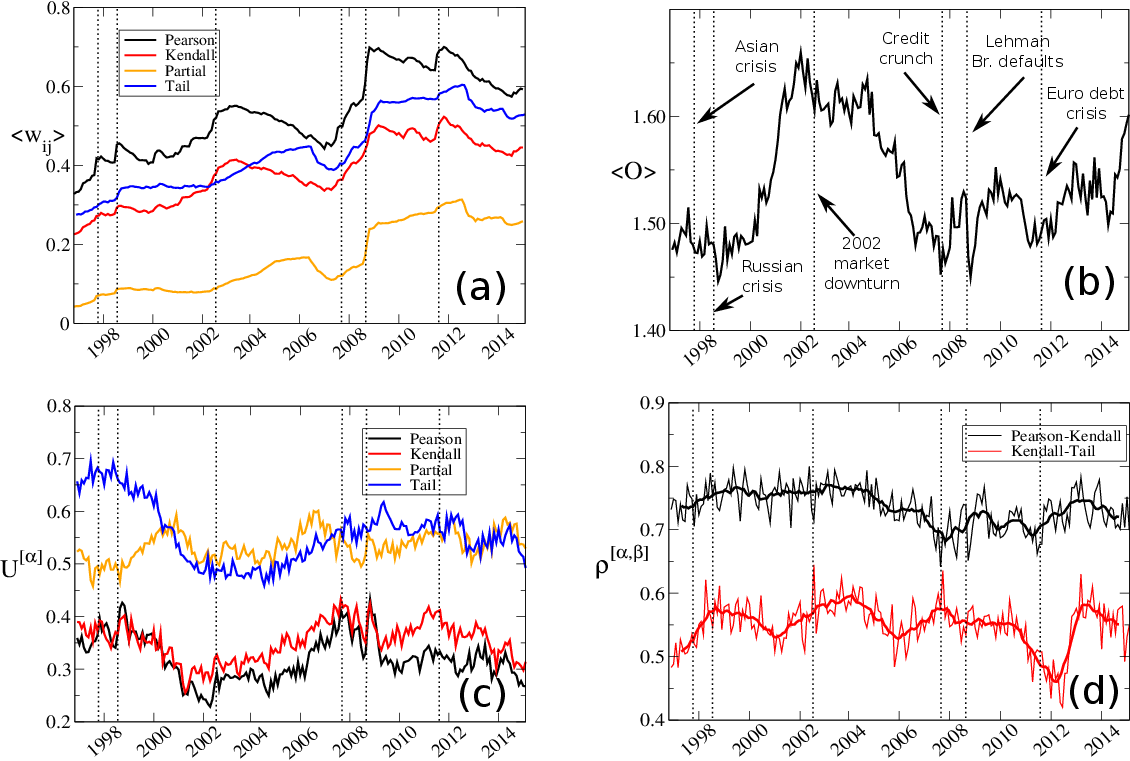
Fig. 1(a) shows how the average link weight of each of the four dependency networks changes over time. These results indicate an overall increase of the typical weights in the examined period 1993-2015 and reveals a strongly correlated behaviour of the four curves (with linear correlation coefficients between the curves range in $[0.91,0.99]$). This strong correlation in the temporal patterns of the four measures of dependence may lead to the wrong conclusion that the four networks carry very similar information about the structure of financial systems. Conversely, we shall see that even basic multiplex measures suggest otherwise. In Fig. 1(b) we report the average edge overlap $\langle O\rangle$, that is the average number of layers of the financial multiplex network where a generic pair of nodes $(i,j)$ is connected by an edge (see Materials and Methods for details). Since our multiplex network consists of four layer, $\langle O\rangle$ takes values in $[1,4]$, and in particular we have $\langle O\rangle=1$ when each edge is present only in one layer, while $\langle O\rangle=4$ when the four networks are identical. The relatively low values of $\langle O\rangle$ observed in this case reveal the complementary role played by the different dependency indicators. It is interesting to note that the edge overlap $\langle O\rangle$ displays a quite dynamic pattern, and its variations seem to be related to the main financial crises highlighted by the vertical lines in Fig. 1(b). The first event that triggers a sensible decrease in the average edge overlap is the Russian crisis in 1998, which corresponds to the overall global minimum of $\langle O\rangle$ in the considered interval. Then, $\langle O\rangle$ starts increasing towards the end of year 2000 and reaches its global maximum at the beginning of 2002, just before the market downturn of the same year. We observe a marked decrease in 2005, in correspondence with the second phase of the housing bubble, which culminates in the dip associated to the credit crunch at the end of 2007. A second, even steeper drop occurs during the Lehman Brothers default of 2008. After that, the signal appears more stable and weakly increasing, especially towards the end of 2014. Since each edge is present, on average, in less than two layers, each of the four layers effectively provides a partial perspective on the dependency structure of the market. This fact is made more evident by the results reported in Fig. 1(c), where we show, for each layer $\alpha=1,\ldots,4$, the fraction of edges $U^{[\alpha]}$ that exist exclusively in that layer (see Materials and Methods for details). We notice that, at any point in time, from $30\%$ to $70\%$ of the edges of each of the four layers are unique to that layer, meaning that a large fraction of the dependence relations captured by a given measure are not captured by the other measures.

Another remarkable finding is that also the relative importance of a stock in the network, measured for instance by its centrality in terms of degree graph_theory ; invest_periph , varies a lot across layers. This is confirmed by the degree correlation coefficient $\rho^{[\alpha,\beta]}$ for pairs of layers $\alpha$ and $\beta$. In general, high values of $\rho^{[\alpha,\beta]}$ signal the presence of strong correlations between the degree of the same node in the two layers (see Materials and Methods for details). Fig. 1(d) shows $\rho^{[\alpha,\beta]}$ as a function of time for two pairs of dependence measures, namely Pearson–Kendall and Kendall–Tail. Notice that the degrees of the layers corresponding to Pearson and Kendall exhibit a relatively large correlation, which remains quite stable over the whole time interval. Conversely, the degrees of nodes in the Kendall and Tail layers are on average less correlated, and the corresponding values of $\rho^{[\alpha,\beta]}$ exhibit larger fluctuations. For example, in the tenth time window we find that General Electric stock (GE US) is a hub in Kendall layer with 71 connections, but it has only 16 connections in the Tail layer: therefore the relevance of this stock in the dependence structure depends sensitively on the layer.

The presence of temporal fluctuations in $\langle O\rangle$, in particular the fact that $\langle O\rangle$ reaches lower values during financial crises, together with the unique patterns of links at each layer, testified by high values of $U^{[\alpha]}$ and by relatively weak inter-layer degree-degree correlations for some pairs of layers, confirm that an analysis of relations among stocks simply based on one dependence measure can neglet relevant information which can however be captured by other measures. As we will show below, a multiplex network approach which takes into account at the same time all the four dependence measures, but without aggregating them into a single-layer network, is able to provide a richer description of financial markets.

Figure 2: Multidegrees reveal the different role of industrial sectors during crises. The plots of the average multidegree of the nodes of the same industrial sector restricted to edges existing exclusively on the (a) Pearson, (b) Kendall, (c) Tail, and (d) Partial layers, clearly show that some dependence measures can reveal structures which are unnoticed by other measures. In particular, the plot of the average multidegree associated to edges existing on at least one layer among Kendall, Tail and Partial, but not on Pearson (panel (e)), reveals that Pearson correlation does not capture many important features such as the prominent role of Basic Materials, Financial, Consumer Goods and Industrials during crises and the increasing importance of Technology and Consumer Services after the 2007-2008 crisis.

Multiedges and node multidegrees.

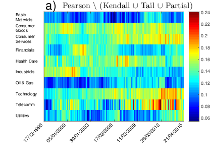
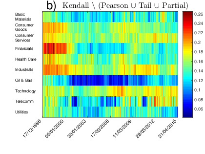
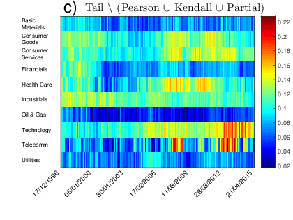
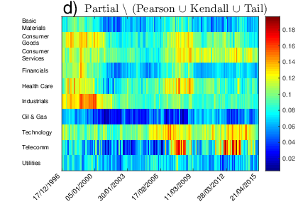
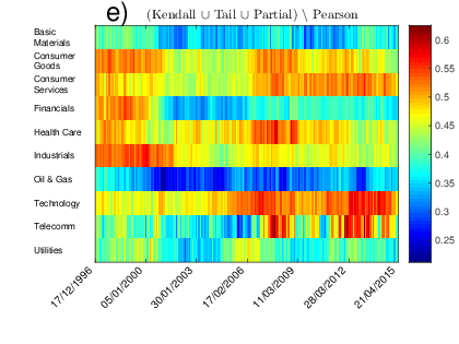
As a first example of useful quantities that can be investigated in a multiplex network, we have computed the so-called multidegree $k_{i}^{\vec{m}}$ for each node $i$ in the network, corresponding to different multiedges (see Materials and Methods) Bianconi2013 . In particular, we have normalised the multidegree of node $i$ dividing it by the corresponding node overlapping degree $o_{i}$, so that the resulting $k_{i}^{\vec{m}}/o_{i}$ is the fraction of multiplex edges of node $i$ that exist only on a given subset of layers. In Fig. 2 we report the average normalised multidegree of each of the 10 industry sectors listed in the ICB classification ICB . We focus on the edges existing exclusively in one of the four layers and on the combination of multi-edges associated to edges existing in either of the Kendall, Tail, or Partial layer, but not in the Pearson layer. As shown in Fig. 2, the multidegree exhibits strong variations in time and high heterogeneity across different industries. Industries such as Oil $\&$ Gas, Utilities, and Basic Materials, show low values of normalised multidegree in all the four panels (a)-(d). Conversely, the edges of nodes corresponding to Industrials, Finance, Technology, Telecommunications, and Consumer Services tend to concentrate in one or in a small subset of layers only. For instance, we observe a relatively high concentration of edges at the Kendall layer for nodes corresponding to Finance, Industrials and Consumer Goods stocks in the period preceding the Dot-com bubble and the 2002 downturn, a feature visible in the Pearson layer in Fig. 2(a). Analogously, we notice a sudden increase of edges unique to the Tail layer for nodes in Consumer Goods, Consumer Services and Health Care after the 2007-2008 crisis. The presence of large heterogeneity and temporal variations in the relative role of different industrial sectors confirms the importance of using a multiplex network approach to analyse dependence among assets.

From this perspective it is particularly interesting to discuss the plot of multidegree restricted to edges that are present on either Kendall, Partial or Tail layer, but are not present in the Pearson layer as reported in Fig. 2(e). Despite the Pearson correlation coefficient is the most used measure to study dependencies, the plot reveals that until 2002 an analysis of the financial network based exclusively on Pearson correlations would have missed from 40$\%$ up to 60$\%$ of the edges of assets in sectors such as Basic Materials, Financial, Consumer Goods and Industrials. The study of evolution with time in Fig. 2(e) reveals that the relative role of such industrial sectors in Kendall, Tail and Partial layers becomes relatively less important between the two crises in 2002 and in 2007, but then such sectors become central again during the 2007-2008 crisis and beyond. This prominent role is quite revealing but it would not had been evident from the analysis of the Pearson layer alone. Let us also note that, the period following the 2007-2008 crisis is also characterised by a sensible and unprecedented increase of the normalised multidegree on Kendall, Partial and Tail layers of stocks belonging to Technology and Telecommunications sectors, whose importance in the market dependence structure has been therefore somehow underestimated over the last ten years by the studies based exclusively on Pearson correlation.

Multiplex cartography of financial systems

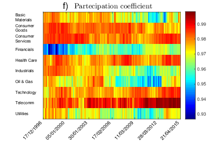
To better quantify the relative importance of specific nodes and groups of nodes we computed the overlapping degree and partecipation coefficient, respectively measuring the total number of edges of a node and how such edges are distributed across the layers (see Materials and Methods for details). We started by computing the average degree $k_{I}^{[\alpha]}$ at layer $\alpha$ of nodes belonging to each ICB industry sector $I$, defined as $k_{I}^{[\alpha]}=\frac{1}{N_{I}}\sum_{i\in I}k_{i}^{[\alpha]}\delta(c_{i},I)$, where by $c_{i}$ we denote the industry of node $i$ and $N_{I}$ is the number of nodes belonging to industry sector $I$. Figs. 3 a)-d) show $k_{I}^{[\alpha]}$ as a function of time for each of the four layers.

Figure 3: Average node degree as a proxy of the importance of an industry. The plots of average degree of the nodes belonging to the different industrial sectors restricted to the (a) Pearson, (b) Kendall, (c) Tail, and (d) Partial layers, and of the average overlapping degree reported in panel (e) confirm the relative importance of Financials. However, the average participation coefficient (panel (f)) suggests that the dependence structure of some sectors such as Basic Materials, Industrials, and Oil & Gas, has become more heterogeneous, i.e., focused only on a subset of the four layers, after the 2007-2008 crisis.

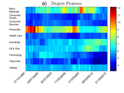
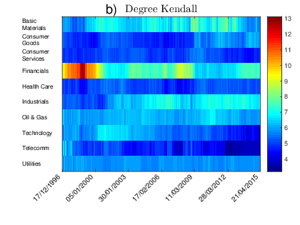
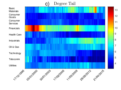
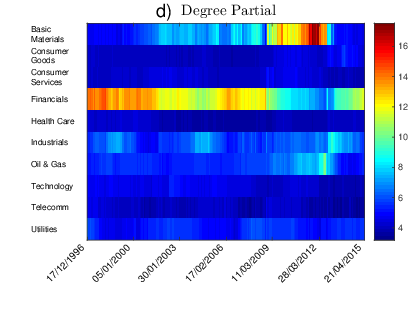
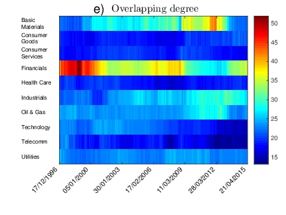
Notice that nodes in the Financial sector exhibit a quite high average degree, no matter the dependence measure used, with a noticeable peak before the Dot-com bubble in 2002. After that, the average degree of Financials has dropped sensibly, with the exception of the 2007-2008 crisis. Apart from the existence of similarities in the overall trend of Financials across the four layers, the analysis of the average degree suggests again the presence of high heterogeneity across sectors and over time.

In the Pearson layer, Basic Materials is the second most central industry throughout most of the observation interval, whereas Industrials and Oil $\&$ Gas acquired more connections in the period following the 2007-2008 crisis. The degree in the Kendall layer is distributed more homogeneously among the sectors than in the Pearson layer. Interestingly, the plot of degree on the Tail layer looks similar to that of the Pearson layer. Finally, in the Partial layer we observe the highest level of concentration of links in Finance (consistently to what found in partial_corr ) and, after the 2007-08 crisis, in Basic Materials.

We have also calculated for each industry $I$ the average overlapping degree $o_{I}\equiv\langle o_{i}\rangle_{i\in I}$, where $o_{i}$ is the overlapping degree of node $i$, which quantifies the overall importance of each industrial sector in the multiplex dependence network. The average overlapping degree of each industry is shown as a function of time in Fig. 3(e). As we can see, $o_{I}$ is able to highlight the prominent role played in the multiplex network by Financials, Basic Materials, Oil & Gas, and Industrials sectors, revealing also the presence of four different phases between 1997 and 2015. The first phase, during which Financials is the only prominent industry, covers the period between 1997 and 2000. The second phase, between 2000 and the 2007-08 crisis, is characterised by the emergence of Basic Materials as the second most central sector. In the third phase, between 2009 and 2014, Financials looses its importance in favour of Industrials, Oil & Gas and Basic Materials (that becomes the most central one). Finally, in 2014 a new equilibrium starts to emerge, with Financials and Industrials gaining again a central role in the system.

The participation coefficient complements the information provided by the overlapping degree, quantifying how the edges of a node are distributed over the layers of the multiplex. In particular, the participation coefficient of node $i$ is equal to $0$ if $i$ has edges in only one of the layers, while it is maximum and equal to $1$ when the edges of node $i$ are equally distributed across the layers (see Materials and Methods for details). In Fig. 3(f) we report, as a function of time, the average participation coefficient $P_{I}$ for each ICB industry $I$. Interestingly, the plot reveals that the increase of the overlapping degrees of Financials, Basic Materials, Industrials, and Oil & Gas sectors shown in Fig. 3(e) are normally accompanied by a substantial decrease of the corresponding participation coefficients. This indicates that those sectors accumulated degree on just one or two layers, confirming what we found in multidegree analysis. A somehow more detailed analysis of the temporal evolution of participation coefficient for each sector is reported in Appendix.

Discussion

By using filtered networks from different correlation measures we have demonstrated that a multiplex network approach can reveal features that would have otherwise been invisible to the analysis of each dependency measure in isolation. Although the layers produced respectively from Pearson, Kendall, Tail and Partial correlations show a certain overall similarity, they exhibit distinct features that are associated with market changes. For instance, we observed that average edge overlap between the first three layers, drops significantly during periods of market stress revealing that non-linear effects are more relevant during crisis periods. The analysis of the average multidegree associated to edges not present on the Pearson layer, but existing on at least one of the three remaining layers, indicates that Pearson correlations alone can miss to detect some important features. We observed that the relative importance of non-linearity and tails on market dependence structure, as measured by mean edge overlap between the last three layers, has dropped significantly in the first half of 2000s and then risen steeply between 2005 and the 2007-08 crisis. Overall, financial crises trigger remarkable drops in the edge overlap, widening therefore the differences among the measures of dependence just when evaluation of risk becomes of the highest importance. Different industry sectors exhibit different structural overlaps. For instance, Financials, Industrials and Consumer Goods show an increasing number of connections only on Kendall layer in the late 90s/early 2000, at the edge of the Dot-Com bubble. After the 2007-08 crisis these industries tend to have many edges on the Kendall, Tail and Partial which are not present on the Pearson layer. This observation questions whether we can rely on the Pearson estimator alone, when analysing correlations between stocks. A study of the overlapping degree and of the participation coefficient shows that asset centrality, an important feature for portfolio optimization invest_periph ; eccentricity_asset , changes considerably across layers with largest desynchronized changes occurring during periods of market distress. Overall our analysis indicates that different dependency measures provide complementary informations about the structure and evolution of markets, and that a multiplex network approach can reveal useful to capture systemic properties that would otherwise go unnoticed.

Materials and Methods

Data set

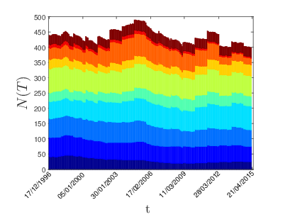
The original dataset consists of the daily prices of $N_{tot}=1004$ US stocks traded in the period between 03/01/1993 and 26/02/2015. Each stock in the dataset has been included in S&P500 at least once in the period considered. Hence the stocks considered provide a representative picture of the US stock market over an extended time window of 22 years, and cover all the 10 industries listed in the Industry Classification Benchmark (ICB) ICB (Fig.4). It is important to notice that most of the stocks in this set are not traded over the entire period. This is a major difference with respect to the majority of the works on dynamic correlation-based networks, in which only stocks continuously traded over the period under study are considered, leading to a significant “survival bias”. For each asset $i$ we have calculated the series of log-returns, defined as $r_{i}(t)=log(P_{i}(t))-log(P_{i}(t-1))$, where $P_{i}(t)$ is stock price at day $t$. The construction of the time-varying multiplex networks is based on log-returns and has been performed in moving time windows of $\theta=1000$ trading days (about 4 years), with a shift of $dT=23$ trading days (about one month), adding up to 200 different multiplex networks, one for each time window. For each time window $T$, four different $N(T)\times N(T)$ dependence matrices have been computed, respectively based on the four different estimators illustrated below. Since the number of active stocks changes with time, dependence matrices at different times can have different number of stocks $N(T)$, as shown in Fig.4. In the figure is also shown the ICB industry composition of our dataset in each time window, confirming that we have a representative sample of all market throughout the period. We have verified that the results we are discussing in the following are robust against change of $\theta$ and $dT$.

Figure 4: Number of stocks in each ICB industry in time. Number of stocks that are continuously traded in each time window together with their partition in terms of ICB industries.

Dependence among financial time series

We have considered four different measures of dependence between two time series $r_{i}(u)$ and $r_{j}(u)$, $i,j=1,2,\ldots,N$, $u=1,2,\ldots,\theta$, indicated in the following respectively as Pearson, Kendall, Tail and Partial.

– Pearson dependence –   It is a measure of linear dependence between two time series, and is based on the evaluation of the Pearson correlation coefficient pearson . We have used the exponentially smoothed version of this estimator exp_smoothing , in order to mitigate excessive sensitiveness to outliers in remote observations:

$$\rho^{w}_{ij}=\frac{\sum_{u=1}^{\theta}w_{u}(r_{i}(u)-\bar{r_{i}}^{w})(r_{j}(u)-\bar{r_{j}}^{w})}{\sqrt{\sum_{u=1}^{\theta}w_{u}(r_{i}(u)-\bar{r_{i}}^{w})^{2}}\sqrt{\sum_{u=1}^{\theta}w_{u}(r_{j}(u)-\bar{r_{j}}^{w})^{2}}}~{}~{},$$ (1)

with

$$w_{u}=w_{0}\exp\left(\frac{u-\theta}{T^{*}}\right)~{}~{},$$ (2)

where $T^{*}$ is the weight characteristic time ($T^{*}>0$) that controls the rate at which past observations lose importance in the correlation, and $w_{0}$ is a constant connected to the normalisation constraint $\sum_{u=1}^{\theta}w_{u}=1$. We have chosen $T^{*}=\theta/3$ according to previously established criteria exp_smoothing .
– Kendall dependence –    It is a measure of dependence that takes into account the nonlinearity of a time series. It is based on the evaluation of the so-called Kendall’s $\tau$ rank correlation coefficient, starting from the quantities $d_{k}(u,v)\equiv sgn(r_{k}(u)-r_{k}(v))$. The estimator counts the number of concordant pairs, i.e. pairs of observations such that $d_{i}(u,v)$ and $d_{j}(u,v)$ have equal signs, minus the number of discordant pairs kendall . As for the case of the Pearson dependence, we have used the exponentially smoothed version of the estimator exp_smoothing :

$$\tau^{w}_{ij}=\sum^{\theta}_{u=1}\sum^{\theta}_{v=u+1}w_{u,v}~{}d_{i}(u,v)d_{j}(u,v)~{}~{},$$ (3)

with

$$w_{u,v}=w_{0}\exp\left(\frac{u-\theta}{T^{*}}\right)\exp\left(\frac{v-\theta}{T^{*}}\right)~{}~{},$$ (4)

where $T^{*}$ is again the weight characteristic time.
– Tail dependence –    It is a non-parametric estimator of tail copula that provides a measure of dependence focused on extreme events. It is based on the evaluation of the following estimator tail_corr :

$$C_{ij}(p_{1},p_{2})=\frac{\sum_{u=1}^{\theta}\mathbbm{1}_{\{F^{i}(r_{i}(u))<p_{1}\wedge F^{j}(r_{j}(u))<p_{2}\}}}{\sum_{u=1}^{\theta}\mathbbm{1}_{\{F^{i}(r_{i}(u))<p_{1}\vee F^{j}(r_{j}(u))<p_{2}\}}}$$ (5)

where $F^{i}$ and $F^{j}$ are the empirical cumulative probabilities of returns $r_{i}(u)$ and $r_{j}(u)$ respectively, $p_{1}$ and $p_{2}$ are two parameters representing the percentiles above which an observation is considered (lower) tail. We focus on lower tails since we are interested in risk management applications, where the attention is on losses. It can be shown that this is a consistent estimator of tail copula tail_corr . In this work we have chosen $p_{1}=p_{2}=0.1$ (i.e. we consider tail every observation below the 10th percentile), as a trade-off between the need of statistic and the interest in extreme events.
– Partial dependence–   It is a measure of dependence that quantifies to what extent each asset affects other assets correlation. The Partial correlation $\rho_{ik|j}$, or correlation influence, between assets $i$ and $k$ based on $j$, is the Pearson correlation between the residuals of $r_{i}(u)$ and $r_{k}(u)$ obtained after regression against $r_{j}(u)$ partial_corr2 . It can be written in terms of a Pearson correlation coefficient as follows partial_corr :

$$\rho_{ik|j}=\frac{\rho_{ik}-\rho_{ij}\rho_{kj}}{\sqrt{[1-\rho_{ij}^{2}][1-\rho_{kj}^{2}]}}$$ (6)

This measure represents the amount of correlation between $i$ and $k$ that is left once the influence of $j$ is subtracted. Following partial_corr , we define the correlation influence of $j$ on the pair $i,k$ as:

$$d(i,k|j)=\rho_{ik}-\rho_{ik|j}$$ (7)

$d(i,k|j)$ is large when a significant fraction of correlation between $i$ and $k$ is due to the influence of $j$. Finally, in order to translate this into a measure between $i$ and $j$, the so-called Partial dependence, we average it over the index $k$:

$$d(i|j)=\langle d(i,k|j)\rangle_{k\neq i,j}$$ (8)

$d(i|j)$ is the measure of influence of $j$ on $i$ based on Partial correlation. It is worth noting that, unlike the other measures of dependence, $d(i|j)$ provides a directed relation between assets (as in general $d(i|j)\neq d(j|i)$). In the rest of the paper we refer to this indicator as “Partial dependence”, even though strictly speaking we are analysing the Correlation influence based on Partial correlation.

Graph filtering and the construction of the multiplex network

For each of the 200 time windows we have then constructed a multiplex network with $M=4$ layers obtained respectively by means of the four dependence indicators. In order to reduce the noise and the redundance contained in each dependence matrix we have applied the Planar Maximally Filtered Graph Tumminello05 PMFG2 PMFG3 TMFG . It is worth mentioning that the filtering of the correlation influence layer requires an adaptation of the PMFG algorithm to deal with asymmetric relations. We have followed the approach suggested in partial_corr that rules out double links between nodes. The obtained planar graphs have been then converted into an undirected graphs and included in the multiplex.

Multiplex measures

Let us consider a weighted multiplex network $\mathcal{M}$ on $N$ nodes, defined by the $M$-dimensional array of weighted adjacency matrices $\mathcal{W}=\{W^{[1]},W^{[2]},\ldots,W^{[M]}\}$, where $W^{[\alpha]}=\{w_{ij}^{[\alpha]}\}$ are the matrices of weights that determine the topology of the $\alpha$-th layer though the PMFG filtering. Here the weight $w_{ij}^{[\alpha]}$ represents the strength of the correlation between node $i$ and node $j$ on layer $\alpha$, where the different layers are obtained through different correlation measures. In the following we will indicate by $W^{[\alpha]}$ the weighted adjacency matrix of the PMFG associated to layer $\alpha$, and by $A^{[\alpha]}$ the corresponding unweighted adjacency matrix, where $a_{ij}^{[\alpha]}=1$ if and only if $w_{ij}^{[\alpha]}\not=0$. We denote by $K^{[\alpha]}=\frac{1}{2}\sum_{ij}a_{ij}^{[\alpha]}$ the number of edges on layer $\alpha$, and by $K=\frac{1}{2}\sum_{i,j}\left[1-\prod_{\alpha}(1-a_{ij}^{[\alpha]})\right]$ the number of pairs of nodes which are connected by at least one edge on at least one of the $M$ layers. Notice that since the network at each layer is a PMFG, then we have $K^{[\alpha]}=3(N-2)\>\forall\alpha$ by construction.

We consider some basic quantities commonly used to characterise multiplex networks Bianconi2013 ; metrics_multiplex . The first one is the mean edge overlap, defined as the average number of layers on which an edge between two randomly chosen nodes $i$ and $j$ exists:

$$\langle O\rangle=\frac{1}{2K}\sum_{i,j}\sum_{\alpha}a_{ij}^{[\alpha]}.$$ (9)

Notice that $\langle O\rangle=1$ only when all the $M$ layers are identical, i.e. $A^{[\alpha]}\equiv A^{[\beta]}\>\forall\alpha,\beta=1,\ldots,M$, while $\langle O\rangle=0$ if no edge is present in more than one layer, so that the average edge overlap is in fact a measure of how much similar is the structure of the layers of a multiplex network. A somehow dual quantity is the fraction of edges of layer $\alpha$ which do not exist on any other layer:

$$U^{[\alpha]}=\frac{1}{2K^{[\alpha]}}\sum_{i,j}a_{ij}^{[\alpha]}\prod_{\beta\neq\alpha}\left(1-a_{ij}^{[\beta]}\right)$$ (10)

which quantifies how peculiar is the structure of a given layer $\alpha$, since $U^{[\alpha]}$ is close to zero only when almost all the edges of layer $\alpha$ are also present on at least one of the other $M-1$ layers.

More accurate information about the contribution of each node to a layer (or to a group of layers) can be obtained by the so-called multidegree of a node $i$. Let us consider the vector $\vec{m}=(m_{1},m_{2},...,m_{M})$, with $M$ equal to the number of layers, where each $m_{\alpha}$ can take only two values $\{1,0\}$. We say that a pair of nodes $i,j$ has a multilink $\vec{m}$ if they are connected only on those layers $\alpha$ for which $m_{\alpha}=1$ in $\vec{m}$ Bianconi2013 . The information on the $M$ adjacency matrices $a_{ij}^{\alpha}$ ($\alpha=1,..,M$) can then be aggregated in the multiadjacency matrix $A_{ij}^{\vec{m}}$, where $A_{ij}^{\vec{m}}=1$ if and only if the pair $i,j$ is connected by a multilink $\vec{m}$. Formally Bianconi2013 ; multiplex_review :

$$A_{ij}^{\vec{m}}\equiv\prod_{\alpha=1}^{M}[a_{ij}^{\alpha}m_{\alpha}+(1-a_{ij}^{\alpha})(1-m_{\alpha})].$$ (11)

From the multiadjacency matrix we can define the multidegree $\vec{m}$ of a node $i$, as the number of multilinks $\vec{m}$ connecting $i$:

$$k_{i}^{\vec{m}}=\sum_{j}A_{ij}^{\vec{m}}.$$ (12)

This measure allows us to calculate e.g. how many edges node $i$ has on layer $1$ only ($k_{i}^{\vec{m}}$ choosing $m_{1}=1$, $m_{\alpha}=0~{}~{}\forall\alpha\neq 1$), integrating the global information provided by $U^{[\alpha]}$.

The most basic measure to quantify the importance of single nodes on each layer is by means of the node degree $k_{i}^{[\alpha]}=\sum_{j}a_{ij}^{[\alpha]}$. However, since the same node $i$ is normally present at all layers, we can introduce two quantities to characterise the role of node $i$ in the multiplexmetrics_multiplex , namely the overlapping degree

$$o_{i}=\sum_{\alpha}k_{i}^{[\alpha]}$$ (13)

and the multiplex participation coefficient:

$$P_{i}=\frac{M}{M-1}\left[1-\sum_{\alpha}\left(\frac{k_{i}^{[\alpha]}}{o_{i}}\right)\right].$$ (14)

The overlapping degree is just the total number of edges incident on node $i$ at any layer, so that node are classified as hubs if they habve a relatively large value of $o_{i}$. The multiplex participation coefficient quantifies the dispersion of the edges incident on node $i$ across the layers. In fact, $P_{i}=0$ if the edges of $i$ are concentrated on exactly one of the $M$ layers (in this case $i$ is a focused node), while $P_{i}=1$ if the edges of $i$ are uniformly distributed across the $M$ layers, i.e. when $k_{i}^{[\alpha]}=\frac{o_{i}}{M}\>\forall\alpha$ (in which case $i$ is a truly multiplex node). The scatter plot of $o_{i}$ and $P_{i}$ is called multiplex cartography and has been used as a synthetic graphical representation of the overall heterogeneity of node roles observed in a multiplex.

In a multiplex network is important also to look at the presence and sign of inter-layer degree correlations. This can be done by computing the inter-layer degree correlation coefficient Nicosia2014correlations :

$$\rho^{[\alpha,\beta]}=\frac{\sum_{i}\left(R^{[\alpha]}_{i}-\overline{R^{[\alpha]}}\right)\left(R^{[\beta]}_{i}-\overline{R^{[\beta]}}\right)}{\sqrt{\sum_{i}\left(R^{[\alpha]}_{i}-\overline{R^{[\alpha]}}\right)^{2}\sum_{j}\left(R^{[\beta]}_{j}-\overline{R^{[\beta]}}\right)^{2}}}$$ (15)

where $R_{i}^{[\alpha]}$ is the rank of node $i$ according to its degree on layer $\alpha$ and $\overline{R^{[\alpha]}}$ is the average rank by degree on layer $\alpha$. In general $\rho^{[\alpha,\beta]}$ takes values in $[-1,1]$, where values close to $+1$ (respectively, $-1$) indicate the of strong positive (resp. negative) correlations, while $\rho^{[\alpha,\beta]}\simeq 0$ if the degrees at the two layers are uncorrelated.

APPENDIX

Time evolution of the average participation coefficient

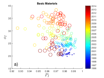
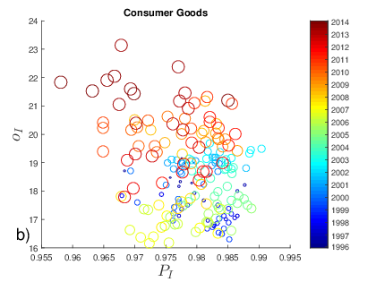
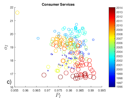
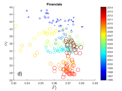
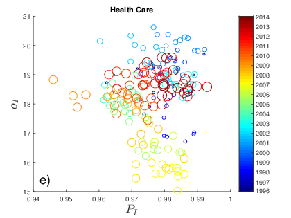
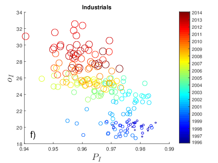
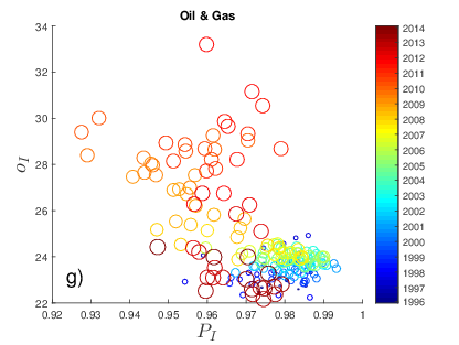
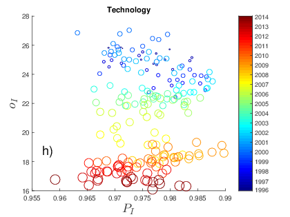
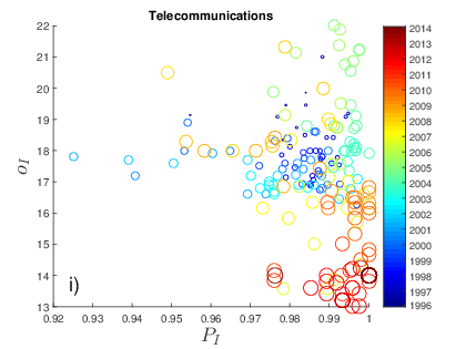
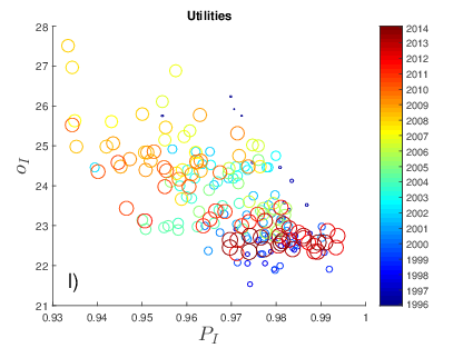
In Fig. 5 we plot the time evolution of the average participation coefficient $P_{I}$ (x-axis) of stocks in the industrial sector $I$ against the average overlapping degree $o_{I}$ (y-axis). Each circle corresponds to one of the 200 time windows, while the size and colour of each circles represent different time windows. Each panel corresponds to one industrial sector $I$. The diagrams reveal that in the last 20 years the role of different sectors has changed radically, and in different directions. For instance, stocks in the Financials sector evolved from a relatively large overlapping degree and a small participation coefficient in the late 1990s, to a smaller number of edges, distributed more homogeneously across the layers, towards the end of the observation period. Conversely, Industrials stocks have acquired degree on some of the layers, resulting in a considerable decrease of participation coefficient. This is another indication of the importance of monitoring all the layers together, as an increase in the structural role of an industry (as measured by the overlapping degree) is typically due to only a subset of layers (as indicated by the corresponding decrease of partecipation coefficient).

Figure 5: Industries evolution in the overlapping degree/partecipation coefficient plane. Fixed an industry $I$, we have plotted for each time window a circle whose $y$ coordinate is the average overlapping degree $o_{I}$ and whose $x$ coordinate is the average partecipation coefficient $P_{I}$. Points at different times are characterized with different sizes (small to large) and colours (legend on the right). In a) - l) we show the results respectively for Basic Materials, Consumer Goods, Consumer Services, Financials, Health Care, Industrials, Oil & Gas, Technology, Telecommunications and Utilities.

Author contributions statement

N.M. and V. N. contributed equally to this work. All the authors devised the study, performed the experiments and simulations, analysed the results, wrote the paper, and approved the final draft.

Additional information

Competing financial interests. The authors declare no competing financial interest.

References

- (1) Mantegna, R. N. Hierarchical structure in financial markets. Eur. Phys. J. B 11, 193 (1999).
- (2) Tumminello, M., Aste, T., Di Matteo, T. & Mantegna, R. A tool for filtering information in complex systems. Proc. Natl. Acad. Sci. 102, 10421–10426 (2005).
- (3) Aste, T., Di Matteo, T. & Hyde, S. T. Complex networks on hyperbolic surfaces. Physica A 346, 20 (2005).
- (4) Aste, T., Di Matteo, T. Dynamical networks from correlations. Physica A 370, 156–161 (2006).
- (5) Aste, T., Grammatica, R. & Di Matteo, T. Exploring complex networks via topological embedding on surfaces. Phys. Rev. E 86, 036109 (2012).
- (6) Boccaletti, S., Latora, V., Moreno, Y., Chavez, M. & Hwang, D.-U. Complex networks: Structure and dynamics. Physics Reports 424, 175 – 308 (2006).
- (7) Massara, G. P., Di Matteo, T. & Aste, T. Network filtering for big data: Triangulated maximally filtered graph. arXiv preprint arXiv:1505.02445, Journal of complex networks (in press) 2016 (2015).
- (8) Barfuss, W., Massara, G. P., Di Matteo, T. & Aste, T. Parsimonious modeling with information filtering networks. arXiv preprint arXiv:1602.07349 (2016).
- (9) Embrechts, P., McNeil, A. & Straumann, D. Correlation and dependency in risk management: Properties and pitfalls. Dempster, M. et al. (Eds.), Risk Management: Value at Risk and Beyond. Cambridge University Press, Cambridge (2001).
- (10) Sornette, D. & Andersen, J. A nonlinear super-exponential rational model of speculative financial bubbles. Int. J. Mod. Phys. C 13, 171–188 (2002).
- (11) Kendall, M. G. A new measure of rank correlation. Biometrika 30, 81–93 (1938).
- (12) Meissner, G. Correlation risk modeling and management. (Harvard University Press, 2014).
- (13) Boccaletti, S. et al. The structure and dynamics of multilayer networks. Phys Rep 544, 1–122 (2014).
- (14) Battiston, F., Nicosia, V. & Latora, V. Metrics for the analysis of multiplex networks. Phys. Rev. E 89, 032804 (2013).
- (15) Nicosia, V. & Latora, V. Measuring and modelling correlations in multiplex networks. Phys. Rev. E 92, 032805 (2015).
- (16) Goffman, E. Frame Analysis: An Essay on the Organization of Experience (Harvard University Press, 1974).
- (17) Szell, M. & Lambiotte, R. & Thurner, S. Multirelational organization of large-scale social networks in an online world. Proc. Natl. Acad. Sci. USA 107, 13636–13641 (2010).
- (18) Klimek, P. & Thurner, S. Triadic closure dynamics drives scaling laws in social multiplex networks. New J. Phys. 15, 063008 (2013).
- (19) Corominas-Murtra, B. & Fuchs, B. & Thurner, S. Detection of the elite structure in a virtual multiplex social system by means of a generalised k-core. Plos One 9, e112606 (2014).
- (20) Tang, L. & Wang, X. & Liu, H. Community detection via heterogeneous interaction analysis. Data Min. Knowl. Discov. 25, 1–33 (2012).
- (21) Kolda, T. G. & Bader, B. W. & Kenny, J. P. Higher-order web link analysis using multilinear algebra. In ICDM 2005: Proc. of the 5th IEEE International Conference on Data Mining, 242–249 (2005).
- (22) Barnett, G. A. & Park, H. W. & Jiang, K. & Tang, C. & Aguillo, I. F. A multi-level network analysis of web- citations among the world’s universities. Scientometrics 99, 5–26 (2014).
- (23) Wu, Z. & Yin, W. & Cao, J. & Xu, G. & Cuzzocrea, A. Community detection in multirelational social networks. In Heidelberg, S. B. (ed.) Web Information Systems Engineering WISE 2013 in Lecture Notes in Computer Science, 8181, 43–56 (2014).
- (24) Buldyrev, S. V. & Parshani, R. & Paul, G. & Stanley, H. E. & Havlin, S. Catastrophic cascade of failures in interdependent networks. Nature 464, 1025–1028 (2010).
- (25) Brummitt, C. D. & D’Souza, R. M. & Leicht, E. A. Suppressing cascades of load in interdependent networks. Proc. Natl. Acad. Sci. USA 109, E680–689 (2012).
- (26) Cardillo, A. & Zanin, M. & Gómez-Gardeñes, J. & Romance, M. & García del Amo, A. & Boccaletti, S. Modeling the multi-layer nature of the european air transport network: Resilience and passengers re-scheduling under random failures. Eur. Phys. J. Spec. Top. 215, 23–33 (2013).
- (27) Barigozzi, M. & Fagiolo, G. & Mangioni, G. Identifying the community structure of the international - trade multi-network. Physica A 390, 2051–2066 (2011).
- (28) Montagna, M. & Kok, C. Multi-layered interbank model for assessing systemic risk, (2013). Kiel Working Paper No.1873.
- (29) Burkholz, R. & Leduc, M. V. & Garas, A. & Schweitzer, F. Systemic risk in multiplex networks with asymmetric coupling and threshold feedback. Physica D (2015).
- (30) Fenn, D. J. et al. Dynamical clustering of exchange rates. Quantitative Finance 12, 1493 (2012).
- (31) Di Matteo, T., Pozzi, F. & Aste, T. The use of dynamical networks to detect the hierarchical organization of financial market sectors. Eur. Phys. J. B 73, 3–11 (2010).
- (32) Aste, T., Shaw, W. & Di Matteo, T. Correlation structure and dynamics in volatile markets. New J. Phys. 12, 085009 (2010).
- (33) Borghesi, C., Marsili, M. & Miccichè, S. Emergence of time-horizon invariant correlation structure in financial returns by subtraction of the market mode. Phys. Rev. E 76, 026104 (2007).
- (34) Musmeci, N., Aste, T. & Di Matteo, T. Relation between financial market structure and the real economy: Comparison between clustering methods. PLoS ONE 10(3): e0116201. doi:10.1371/journal.pone. 011620125786703 (2015).
- (35) Onnela, J. P., Chakraborti, A., Kaski, K. & Kertész, J. Dynamic asset trees and black monday. Physica A 324, 247–252 (2003).
- (36) Musmeci, N., Aste, T. & Di Matteo, T. Risk diversification: a study of persistence with a filtered correlation-network approach. Journal of Network Theory in Finance 1, 1–22 (2015).
- (37) Musmeci, N., Aste, T. & Di Matteo, T. What does past correlation structure tell us about the future? An answer from network theory. Submitted (2016).
- (38) Tola, V., Lillo, F., Gallegati, M. & Mantegna, R. Cluster analysis for portfolio optimization. J. Econ. Dyn. Control 32, 235–258 (2008).
- (39) Pozzi, F. & Di Matteo, T. & Aste, T. Spread of risk across financial markets: better to invest in the peripheries. Scientific Reports DOI:10.1038/srep01665 3, 1665 (2013).
- (40) Kenett, D. Y. et al. Dominating clasp of the financial sector revealed by partial correlation analysis of the stock market. PLoS ONE 5, e15032. doi:10.1371/journal.pone.0015032 (2010).
- (41) West, D. B. Introduction to graph theory (Prentice-Hall, Englewood Cliffs NJ, 1996).
- (42) Bianconi, G. Statistical mechanics of multiplex networks: Entropy and overlap. Phys. Rev. E 87, 062806 (2013).
- (43) A Guide to Industry Classification Benchmark. Available at:. http://www.icbenchmark.com/.
- (44) Onnela, J.-P., Chakraborti, A., Kaski, K., Kertész, J. & Kanto, A. Dynamics of market correlations: Taxonomy and portfolio analysis. Phys. Rev. E 68, 056110 (2003).
- (45) Kaya, H. Eccentricity in asset management. Journal of Network Theory in Finance 1, 45–76 (2015).
- (46) Pearson, K. Notes on regression and inheritance in the case of two parents. Proceedings of the Royal Society of London 58, 240–242 (1895).
- (47) Pozzi, F., Di Matteo, T. & Aste, T. Exponential smoothing weighted correlations. Eur. Phys. J. B 85, 6 (2012).
- (48) Schmidt, R. & Stadmüller, U.. Nonparametric estimation of tail dependence. Scandinavian Journal of Statistics 33, 307–335 (2006).
- (49) Baba, K., Shibata, R. & Sibuya, M. Partial correlation and conditional correlation as measures of conditional independence. Australian & New Zealand Journal of Statistics 46, 657–664 (2004).
Acknowledgments
The authors wish to thank Alessandro Fiasconaro for useful discussions at the beginning of this project. V.L. acknowledges support from the EPSRC project GALE, EP/K020633/1. The authors wish to thank Bloomberg for providing the data. TDM wishes to thank the COST Action TD1210 for partially supporting this work.