Exploring AGN - starburst coexistence in galaxies at
z$\sim$ 0.8 by the [OIII]4959+5007/[OIII]4363 line ratio

Abstract

We analyse by detailed modelling the spectra observed from the sample galaxies at z$\sim$0.8 presented by Ly et al (2015), constraining the models by the [OIII]5007+4959/[OIII]4363 line ratios. Composite models (shock + photoionization) are adopted. Shock velocities $\geq$ 100 $\rm km\,s^{-1}$and preshock densities $\rm n_{0}$$\sim$ 200 $\rm cm^{-3}$ characterize the gas surrounding the starburst (SB), while $\rm n_{0}$ are higher by a factor of 1.5-10 in the AGN emitting gas. SB effective temperatures are similar to those of quiescent galaxies ($\rm T_{*}$ $\sim$4-7 10⁴ K). Cloud geometrical thickness in the SB are $\leq$ 10¹⁶ cm indicating major fragmentation, while in AGN they reach $>$ 10 pc. O/H are about solar for all the objects, except for a few AGN clouds with O/H= 0.3 -0.5 solar. Starburst models reproduce most of the data within the observational errors. About half of the object spectra are well fitted by an accreting AGN. Some galaxies show multiple radiation sources, such as SB+AGN, or a double AGN.

1 Introduction

Starburst (SB) - active galactic nucleus (AGN) connection is generally explored in order to understand galaxy formation, structure and evolution. Processes which stimulate starbursts may lead also to AGN onset (Hopkins et al 2011). Dixon & Joseph (2011) using a variety of spectroscopic diagnostics found that $\sim$50% of the luminous infrared galaxies (LIRG) in their sample shows some evidence for an AGN. The luminosity of $\sim$ 17 % of the sample galaxies seems dominated by emission from AGN, and the remaining $\sim$ 80 % have luminosities dominated by SB. $\sim$50% of the sample galaxies indicates coupled AGN and starburst activities suggesting that AGNs and starbursts commonly coexist. Contini & Contini (2007) investigating a sample of LIRG (L_IR $>$10¹¹L_⊙ ), ultra-LIRG (ULIRG, L_IR $>$10¹²L_⊙ ) and hyper-LIRG (HLIRG,L_IR $>$ 10¹³L_⊙ ) concluded that half of the LIRG contains an AGN, at least one AGN is found in all the ULIRG and none in the HLIRG. The connection between the AGN and the starburst is not direct and it is affected by a (viscous) time lag of gas flowing through the AGN accretion disc leading to AGN activity delay in star formation activity (Blank & Duschl 2013). AGN feedback may terminate star formation in the host galaxy poor gas phase and trigger it in the rich phase (Zubovas et al. 2013). SB-AGN coexistence in local galaxies has been investigated by the analysis of mid-infrared lines and of the continuum spectral energy distribution (SED) adopting diagnostic diagrams (e.g. Dixon & Joseph 2011) and by the optical- UV lines and continuum SED in relatively high z galaxies by detail modelling (Contini 2015 and references therein).

In this paper we revisit the spectra from galaxies at z$\sim$0.8, presented by the Ly et al (2015) DEEP2 survey. The observations were done by the DEIMOS multi-object spectrograph on the Keck II telescope. The observed spectra account for the [OIII]5007+ (the + indicates that the 5007 and 4959 lines are summed), [OIII]4363, [NeIII] 3869+, [OII]3727+, and H${\beta}$ lines which can be used to constrain the models. The observed spectra are generally reproduced by detailed modelling. We have noticed by modelling the spectra observed from many different galaxy types (Contini 2016 and references therein), that in some cases, even when the [OIII]5007+/H${\beta}$ and [OII]3727+/H${\beta}$ line ratios are well fitted by the models, the [OIII]4363/H${\beta}$ systematically disagree. For instance, [OIII] 4363/H${\beta}$ line ratios calculated by shock dominated models overpredict the data in super-luminous SN host galaxies (Contini 2016). Therefore, the [OIII]4363/H${\beta}$ line ratios, when available, are useful to constrain the models. Selecting the AGN, SB, and/or only shock dominated models best fitting the data, the galaxy types can be distinguished.

The R_[OIII] ([OIII]5007+4959/[OIII]4363) line ratios are favourite in the modelling process because they depend only indirectly on the O/H relative abundance. Actually, O/H variations affect the cooling process in the recombination zone of the emitting clouds leading to different line spectra. We use models which account for both the photoionizing flux from a primary radiation source and shocks. Shocks yield fragmentation of matter by turbulence created near the shock-front and compression of the gas downstream, leading to high densities which can trigger star formation. Composite models resolved the problem regarding R_[OIII] in AGN and LINER (low-ionization nuclear emission-line region) spectra, which indicated relatively high temperatures ($>$ 10⁵K) and densities ($>$ 10⁵ $\rm cm^{-3}$) in the emitting gas (Contini & Aldrovandi 1986). Moreover, comparing calculated with observed line ratios the gas motion direction can be determined, i.e. infalling towards the radiation source or ejected outwards (Fig. 1). This is an important issue in view of the SB - AGN feedback in galaxies. The calculation method is described in Sect. 2. Model results are compared with the data in Sect. 3. Discussion and concluding remarks appear in Sect. 4.

2 Calculation of the spectra

Figure 1: Case a) : the cloud withdraws from the radiation source which is represented by the star; case b) the cloud approaches the radiation source

Figure 2: Top : log([OIII]5007+/H${\beta}$ ) (obs) vs log([OII]3727+/H${\beta}$ ) (obs); bottom : log([OIII]4363)/H${\beta}$ (obs) vs log([OII]3727+/H${\beta}$ ) (obs)

Spectroscopic data provide a full physical and chemical picture for local galaxies. At high redshifts the data are reduced to a few significant lines, but the surveys contain hundreds of objects. Therefore, in order to obtain the O/H metallicity, the oxygen line ratios are generally calculated by the ”direct methods” (see e.g. Ly et al 2015, Modjaz et al 2008). The ”direct” or $\rm T_{e}$  method (Seaton 1975, Pagel et al. 1992, etc) was used to obtain O/H from the observed oxygen to H${\beta}$ line ratios. By this method, the ranges of the gas physical conditions are chosen among those most suitable to the observed line ratios. The [OIII]4363 line derives from the upper ${}^{1}S$ level, while [OIII] 4959 and 5007 lines derive from the lower ${}^{1}D$ level. The relative rates of excitation of the ${}^{1}S$ and ${}^{1}D$ levels depend very strongly on the temperature T (Osterbrock 1974). Therefore, T is calculated from the [OIII]5007+/[OIII] 4363 ratio, which depends also on the gas density. This is generally obtained from the [SII] 6717/6730 line ratios. In the present spectra the [SII]6717,6731 lines were not observed. Moreover, by ”direct methods” a unique temperature is adopted throughout the whole galaxy, neglecting the physical conditions less adapted to the strongest lines. This leads to discrepancies between metallicities (in terms of the O/H relative abundance) calculated by ”direct methods” and detailed modelling (see, e.g. Contini 2014a), because the gas cools and recombines in the regions far from the photoionization source, as well as downstream of shock-fronts. By detailed modelling the gas at low (T$<$ 10⁴K) temperatures contributes to the line emission. The line fluxes which result from integration throughout regions of gas at various temperatures are different from those calculated by an homogeneous temperature. If the fractional abundances of the corresponding ions are low, relatively high O/H are needed to reproduce strong oxygen observed lines. So, the metallicities calculated by detailed modelling are generally higher than those calculated by ”direct methods”. A comparison between the results obtained by ”direct methods” and detailed modelling (Contini 2014a) demonstrates that ”direct methods” lead to O/H lower limits.

Detailed modelling of the spectra by pure photoionization models (e.g. by the CLOUDY code) gives satisfying results for intermediate ionization level lines. However, galaxies at high redshifts often originate from mergers and show a disturbed hydrodynamic structure. Collisional phenomena are critical in the calculation of the spectra. We suggest that models based on the coupled effect of photoionization and shocks are the closest approximation to the complex structure of the emitting gas. Therefore, the SUMA code (Contini 2015 and references therein) is used.

The code simulates the physical conditions in an emitting gaseous cloud under the coupled effect of photoionization from the primary radiation source ( SB or AGN) and shocks. The line and continuum emission from the gas are calculated consistently with dust-reprocessed radiation in a plane-parallel geometry. The calculations start at the shock front where the gas is compressed and thermalized adiabatically, reaching the maximum temperature in the immediate post-shock region ($T(K)\sim 1.5\times 10^{5}/(V_{\rm s}/100$ km s^-1$)^{2}$, where $\rm V_{s}$ is the shock velocity). T decreases downstream following the cooling rate. The input parameters such as $\rm V_{s}$ , the atomic preshock density $\rm n_{0}$ and the preshock magnetic field $\rm B_{0}$ (for all models $\rm B_{0}$=10^-4Gauss is adopted) define the hydrodynamical field.

The input parameters that represent the primary radiation for a SB are the effective temperature $\rm T_{*}$ and the ionization parameter $U$. For an AGN, the primary radiation is the power-law radiation flux from the active center $F$ in number of photons cm^-2 s^-1 eV^-1 at the Lyman limit and spectral indices $\alpha_{UV}$=-1.5 and $\alpha_{X}$=-0.7. The primary radiation source is independent but it affects the surrounding gas. In contrast, the secondary diffuse radiation is emitted from the slabs of gas heated by the radiation flux reaching the gas and, in particular, by the shock. In our model the gas region surrounding the radiation source is not considered as a unique cloud, but as an ensemble of fragmented filaments. The geometrical thickness of these filaments is an input parameter of the code (D) which is calculated consistently with the physical conditions and element abundances of the emitting gas. Primary and secondary radiations are calculated by radiation transfer throughout the slabs downstream. The fractional abundances of the ions are calculated resolving the ionization equations. The dust-to-gas ratio ($d/g$) and the abundances of He, C, N, O, Ne, Mg, Si, S, A, Fe, relative to H, are also accounted for.

In the modelling process, we aim to reproduce the observed line ratios for each element. Each line has a different strength which translates into the different precision by the fitting process. A minimum number of significant lines ([OIII] 5007+, [OII]3727+, [OIII]4363, [NII], H${\beta}$ , H${\alpha}$ ) is necessary to constrain the model but the number of the observed lines does not interfere with the modelling process. We deal with line ratios to avoid distance and morphological effects. We start adopting solar abundances by Allen (1976) in the first modelling trials because their values are between the two more recent ones by Anders & Grevesse (1989) and Asplund et al (2009). A perfect fit of the observed line ratios is not realistic because the observed data have errors, both random and systematic. The uncertainty in the calculation is due to the atomic parameters (within 10 %) which are often updated. The strongest lines are reproduced by $<$ 10%, the weakest by $\sim$ 50 %. The calculation code and our modelling method are described by Contini (2014a, 2016 and references therein).

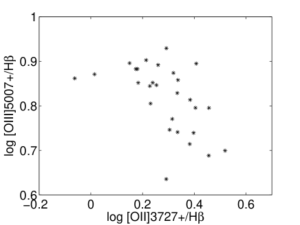
Before starting the modelling process of the present survey galaxies, some characteristics can be guessed by comparing different line ratios in Fig. 2. The top diagram shows that excluding three objects (ID 4, 15 and 16) the slope shown by the line ratio band suggests that a radiation mechanism should be adopted. In the bottom diagram, excluding three objects (ID 4, 8 and 15), a well defined slope is not seen. This reveals large ranges of temperatures and densities in the emitting gas, indicating that other mechanisms such as e.g. shocks could be at work.

Figure 3: Comparison of our models with Kewley et al diagrams. red filled circles: SB models; blue circles : AGN infalling models; black squares : AGN outflow models.

3 Modelling results

Table 1: Comparison of observed line ratios to H${\beta}$ with model results

ID	z	FWHM1	H${\beta}$ 2	[OII]3726+3728/H${\beta}$	[NeIII]3869/H${\beta}$	H${\gamma}$ /H${\beta}$	[OIII]4363/H${\beta}$	[OIII]4959+5007/H${\beta}$ (corr)	R[OIII]
1	0.819	170.9	6.610	2.165${}_{-0.051}^{+0.101}$	0.409${}_{-0.040}^{+0.040}$	0.474${}_{-0.021}^{+0.019}$	0.090${}_{-0.018}^{+0.018}$	5.507${}_{-0.067}^{+0.156}$ (5.15)	57.27${}_{-8.8}^{+11.75}$
MSB1	-	-	-	1.800	0.300	0.460	0.100	5.000	50.
Mpl1	-	-	-	2.180	0.590	0.450	0.030	5.600	186.66
Mpl01	-	-	-	2.050	0.500	0.460	0.030	5.110	170.3
2	0.749	87.300	5.070	1.821${}_{-0.235}^{+0.705}$	0.465${}_{-0.075}^{+0.151}$	-	0.101${}_{-0.020}^{+0.016}$	7.792${}_{-0.351}^{+0.200}$ (6.85)	67.84${}_{-6.62}^{+19.856}$
MSB2				1.800	0.561	0.450	0.200	7.200	36.
Mpl2				1.900	0.700	0.450	0.045	7.400	164.44
Mpl02				1.900	0.400	0.450	0.041	6.990	170.48
3	0.710	109.2	4.510	2.413${}_{-0.103}^{+0.103}$	0.475${}_{-0.043}^{+0.085}$	0.484${}_{-0.029}^{+0.022}$	0.081${}_{-0.023}^{+0.018}$	5.178${}_{-0.085}^{+0.198}$ (4.45)	54.98${}_{-10.47}^{+20.95}$
MSB3				2.400	0.320	0.460	0.075	4.500	60.
Mpl3				2.200	0.600	0.440	0.050	5.000	100.
Mpl03				2.200	0.400	0.500	0.040	4.770	119.25
4	0.788	83.2	3.690	0.867${}_{-0.094}^{+0.094}$	0.187${}_{-0.066}^{+0.066}$	-	0.275${}_{-0.063}^{+0.079}$	7.273${}_{-0.578}^{+0.385}$ (5.0)	18.19${}_{-1.692}^{+5.923}$
MSB4				1.100	0.300	0.450	0.200	5.000	25.
Mpl4				0.990	0.260	0.440	0.072	5.120	71.1
Mpl04				0.820	0.160	0.43	0.450	5.100	11.33
5	0.771	105.7	19.620	1.960${}_{-0.084}^{+0.084}$	0.552${}_{-0.022}^{+0.017}$	0.468${}_{-0.008}^{+0.006}$	0.087${}_{-0.009}^{+0.007}$	8.497${}_{-0.053}^{+0.080}$ (7.87)	90.48${}_{-8.133}^{+10.167}$
MSB5				1.940	0.500	0.450	0.150	8.000	53.3
Mpl5				1.760	0.560	0.460	0.052	7.890	151.7
Mpl05				2.000	0.510	0.460	0.310	8.090	26.1
6	0.717	99.8	11.240	2.539${}_{-0.095}^{+0.221}$	0.403${}_{-0.020}^{+0.035}$	0.468${}_{-0.007}^{+0.016}$	0.038${}_{-0.005}^{+0.011}$	6.245${}_{-0.081}^{+0.081}$ (4.99)	131.24${}_{-15.91}^{+47.72}$
MSB6				2.500	0.350	0.460	0.055	4.930	89.6
Mpl6				2.460	0.460	0.443	0.028	5.19	185.7
Mpl06				2.473	0.460	0.460	0.050	5.200	104.
7	0.762	108.5	12.810	3.304${}_{-0.260}^{+0.208}$	0.410${}_{-0.025}^{+0.032}$	-	0.047${}_{-0.012}^{+0.021}$	5.003${}_{-0.081}^{+0.040}$ (3.9)	83.49${}_{-12.85}^{+25.69}$
MSB7				3.400	0.420	0.460	0.170	4.100	24.1
Mpl7				3.100	0.420	0.440	0.040	4.200	105.
Mpl07				3.300	0.460	0.460	0.180	4.100	22.78
8	0.765	83.7	2.700	1.412${}_{-0.097}^{+0.779}$	0.112${}_{-0.029}^{+0.058}$	-	0.272${}_{-0.062}^{+0.078}$	7.866${}_{-0.168}^{+0.589}$ (6.59)	24.25${}_{-4.217}^{+8.434}$
MSB8				1.860	0.200	0.460	0.290	6.500	22.4
Mpl8				1.300	0.227	0.444	0.070	7.000	100.
Mpl08				1.540	0.180	0.460	0.263	6.760	25.7
9	0.791	143.500	6.360	2.496${}_{-0.079}^{+0.197}$	0.380${}_{-0.048}^{+0.040}$	0.468${}_{-0.020}^{+0.017}$	0.052${}_{-0.009}^{+0.022}$	5.485${}_{-0.099}^{+0.124}$ (4.09)	78.65${}_{-14.98}^{29.964}$
MSB9				2.400	0.300	0.460	0.066	4.160	59.4
Mpl9				2.600	0.380	0.440	0.040	4.000	100.
Mpl09				2.100	0.420	0.460	0.053	4.500	84.9
10	0.794	109.1	12.910	2.159${}_{-0.140}^{+0.093}$	0.435${}_{-0.026}^{+0.017}$	0.468${}_{-0.01}^{+0.008}$	0.077${}_{-0.014}^{+0.009}$	6.739${}_{-0.04}^{+0.094}$ (6.55)	85.11${}_{-12.38}^{+15.474}$
MSB10				2.300	0.477	0.460	0.080	6.750	84.4
Mpl10				2.000	0.490	0.440	0.040	6.690	167.25
Mpl010				2.200	0.400	0.460	0.075	6.400	85.3
11	0.798	86.3	5.400	2.086${}_{-0.065}^{+0.065}$	0.509${}_{-0.062}^{+0.035}$	0.474${}_{-0.020}^{+0.014}$	0.123${}_{-0.011}^{+0.025}$	7.48${}_{-0.118}^{0.148}$ (7.17)	58.30${}_{-11.18}^{+3.195}$
MSB11				2.100	0.490	0.460	0.090	7.200	80.
Mpl11				2.160	0.490	0.460	0.060	7.140	119.
Mpl011				2.060	0.530	0.460	0.086	7.300	84.9
12	0.749	105.5	7.910	1.702${}_{-0.0}^{+0.229}$	0.482${}_{-0.039}^{+0.046}$	0.468${}_{-0.017}^{+0.020}$	0.090${}_{-0.009}^{+0.007}$	6.384${}_{-0.056}^{+0.130}$ (6.39)	70.87${}_{-5.956}^{+4.756}$
MSB12				1.900	0.420	0.460	0.060	6.340	105.7
Mpl12				1.850	0.470	0.460	0.050	6.500	130.
Mpl012				1.700	0.470	0.460	0.080	6.760	84.5
13	0.794	91.200	4.050	2.862${}_{-0.185}^{+0.369}$	0.459${}_{-0.035}^{+0.052}$	0.468${}_{-0.020}^{+0.016}$	0.075${}_{-0.015}^{+0.015}$	6.241${}_{-0.103}^{+0.154}$ (5.58)	74.34${}_{-11.437}^{15.25}$
MSB13				2.600	0.460	0.460	0.090	6.250	69.4
Mpl13				3.000	0.470	0.460	0.034	5.640	165.88
Mpl013				2.500	0.430	0.460	0.060	5.800	96.66
14	0.794	190.900	16.990	2.173${}_{-0.089}^{+0.089}$	0.476${}_{-0.021}^{+0.017}$	0.468${}_{-0.009}^{+0.009}$	0.066${}_{-0.007}^{+0.007}$	7.209${}_{-0.040}^{+0.040}$ (6.94)	105.147${}_{-9.669}^{+12.09}$
MSB14				2.300	0.490	0.460	0.090	7.130	79.2
Mpl14				2.120	0.540	0.455	0.043	7.020	163.25
Mpl014				2.240	0.477	0.460	0.078	7.220	92.56
15	0.755	132.8	12.520	1.034${}_{-0.027}^{+0.096}$	0.480${}_{-0.012}^{+0.040}$	-	0.098${}_{-0.008}^{+0.008}$	7.428${}_{-0.042}^{+0.084}$ (7.06)	72.096${}_{-6.92}^{+4.614}$
MSB15				1.000	0.340	0.460	0.180	7.400	41.1
Mpl15				1.000	0.540	0.440	0.070	7.200	102.85
Mpl015				1.070	0.540	0.460	0.080	6.940	86.75

¹ in $\rm km\,s^{-1}$; ² in 10^-17 $\rm erg\,cm^{-2}\,s^{-1}$;

Table 1-continued

ID	z	FWHM	H${\beta}$	[OII]3726+3728/H${\beta}$	[NeIII]3869/H${\beta}$	H${\gamma}$ /H${\beta}$	[OIII]4363/H${\beta}$	[OIII]4959+5007/H${\beta}$ (corr)	R[OIII]
16	0.774	205.9	8.700	1.958${}_{-0.00}^{+0.945}$	0.272${}_{-0.059}^{+0.073}$	-	0.064${}_{-0.005}^{+0.041}$	4.320${}_{-0.124}^{+0.124}$ (3.4)	46.844${}_{-12.49}^{+18.738}$
MSB16				2.100	0.230	0.460	0.090	3.270	36.3
Mpl16				1.850	0.303	0.440	0.027	3.500	129.6
Mpl016				1.600	0.230	0.460	0.040	3.870	96.75
17	0.764	132.7	7.130	2.420${}_{-0.074}^{+0.596}$	0.618${}_{-0.048}^{+0.096}$	-	0.064${}_{-0.013}^{+0.016}$	6.508${}_{-0.074}^{+0.147}$ (5.73)	89.58${}_{-17.34}^{+28.898}$
MSB17				2.500	0.560	0.460	0.065	6.100	93.8
Mpl17				2.420	0.670	0.440	0.060	5.930	98.83
Mpl017				2.300	0.640	0.460	0.050	5.500	110.
18	0.789	136.4	9.300	1.794${}_{-0.194}^{+0.129}$	0.553${}_{-0.031}^{+0.072}$	0.468${}_{-0.020}^{+0.021}$	0.053${}_{-0.012}^{+0.012}$	7.022${}_{-0.113}^{+0.113}$ (6.12)	115.5${}_{-14.9}^{+37.258}$
MSB18				1.800	0.500	0.460	0.040	6.200	155.
Mpl18				1.830	0.630	0.450	0.036	6.200	172.2
Mpl018				2.000	0.520	0.460	0.051	5.900	115.7
19	0.856	144.0	14.510	1.636${}_{-0.026}^{+0.021}$	0.263${}_{-0.007}^{+0.024}$	0.596${}_{-0.015}^{+0.018}$	0.045${}_{-0.006}^{+0.013}$	7.989${}_{-0.132}^{+0.066}$ (5.8)	128.95${}_{-23.99}^{+17.99}$
MSB19				1.800	0.270	0.460	0.040	5.870	146.7
Mpl19				1.470	0.230	0.440	0.057	5.850	102.6
Mpl019				1.500	0.210	0.460	0.073	6.190	84.93
20	0.784	108.0	6.820	2.017${}_{-0.221}^{+0.276}$	0.267${}_{-0.023}^{+0.046}$	0.468${}_{-0.024}^{+0.030}$	0.135${}_{-0.039}^{+0.026}$	5.575${}_{-0.159}^{+0.132}$ (4.90)	36.499${}_{-5.84}^{+14.6}$
MSB20				2.300	0.300	0.460	0.127	4.830	38.
Mpl20				1.800	0.350	0.440	0.054	5.200	96.3
Mpl020				1.940	0.490	0.460	0.054	4.960	91.85
21	0.823	110.9	5.580	1.692${}_{-0.115}^{+0.344}$	0.423${}_{-0.046}^{+0.108}$	0.468${}_{-0.034}^{+0.032}$	0.120${}_{-0.026}^{+0.026}$	6.989${}_{-0.223}^{+0.179}$ (6.29)	52.46${}_{-8.507}^{+11.343}$
MSB21				1.800	0.470	0.460	0.135	6.290	46.6
Mpl21				1.580	0.390	0.450	0.040	6.300	157.5
Mpl021				1.900	0.580	0.460	0.07	6.300	90.
22	0.784	85.0	6.360	1.735${}_{-0.043}^{+0.343}$	0.429${}_{-0.043}^{+0.054}$	0.468${}_{-0.021}^{+0.028}$	0.112${}_{-0.028}^{+0.008}$	7.110${}_{-0.207}^{+0.103}$ (6.9)	61.69${}_{-9.49}^{+12.654}$
MSB22				1.770	0.450	0.460	0.120	7.100	59.17
Mpl22				1.760	0.390	0.450	0.040	7.170	179.25
Mpl022				1.900	0.440	0.460	0.073	7.000	95.9
23	0.766	97.6	7.670	1.492${}_{-0.00}^{+0.720}$	0.369${}_{-0.060}^{+0.100}$	-	0.059${}_{-0.019}^{+0.015}$	7.631${}_{-0.108}^{+0.135}$ (8.5)	144.017${}_{-57.607}^{+0.0}$
MSB23				1.700	0.480	0.460	0.034	7.700	226.47
Mpl23				1.600	0.447	0.450	0.050	8.300	166.
Mpl023				1.500	0.460	0.460	0.080	8.300	97.6
24	0.721	83.1	14.890	1.525${}_{-0.076}^{+0.076}$	0.409${}_{-0.008}^{+0.027}$	0.468${}_{-0.009}^{+0.008}$	0.073${}_{-0.008}^{+0.009}$	7.105${}_{-0.057}^{+0.057}$ (6.93)	94.92${}_{-10.43}^{+8.344}$
MSB24				1.520	0.410	0.460	0.040	7.160	179.
Mpl24				1.500	0.400	0.450	0.043	7.200	167.4
Mpl024				1.610	0.480	0.460	0.075	6.900	92.0
25	0.789	102.4	7.330	2.857${}_{-0.336}^{+0.269}$	0.530${}_{-0.038}^{+0.077}$	0.468${}_{-0.026}^{+0.024}$	0.091${}_{-0.015}^{+0.012}$	4.878${}_{-0.065}^{+0.130}$ (4.42)	48.60${}_{-8.526}^{+5.116}$
MSB25				2.700	0.450	0.460	0.073	4.850	69.3
Mpl25				2.900	0.600	0.450	0.022	4.700	213.6
Mpl025				2.500	0.580	0.460	0.053	4.700	88.7
26	0.774	109.2	15.690	2.064${}_{-0.041}^{+0.031}$	0.309${}_{-0.020}^{+0.020}$	0.479${}_{-0.011}^{+0.014}$	0.053${}_{-0.008}^{+0.006}$	5.895${}_{-0.044}^{+0.089}$ (5.78)	109.09${}_{-14.307}^{+14.307}$
MSB26				2.100	0.400	0.460	0.043	6.200	144.18
Mpl26				2.880	0.390	0.450	0.044	6.000	136.4
Mpl026				2.000	0.370	0.460	0.057	5.730	100.5
27	0.729	86.4	7.120	2.555${}_{-0.330}^{+0.220}$	0.479${}_{-0.033}^{+0.077}$	0.468${}_{-0.021}^{+0.017}$	0.125${}_{-0.012}^{+0.024}$	7.849${}_{-0.231}^{+0.132}$ (6.87)	54.97${}_{-7.715}^{+9.644}$
MSB27				2.300	0.460	0.460	0.136	6.600	48.5
Mpl27				2.340	0.440	0.460	0.050	7.170	143.4
Mpl027				2.440	0.530	0.460	0.080	7.000	87.5
28	0.732	114.5	22.760	1.515${}_{-0.028}^{+0.042}$	0.504${}_{-0.009}^{+0.014}$	0.468${}_{-0.004}^{+0.006}$	0.056${}_{-0.005}^{+0.002}$	7.633${}_{-0.019}^{+0.037}$ (7.42)	132.44${}_{-5.333}^{+10.667}$
MSB28				1.500	0.420	0.460	0.045	7.500	166.7
Mpl28				1.540	0.500	0.440	0.044	7.600	172.7
Mpl028				1.500	0.500	0.460	0.090	7.540	83.78

Table 2: Description of models MSB1-MSB28

mod	$\rm V_{s}$	$\rm n_{0}$	$\rm T_{*}$	$U$	$D$	O/H	Ne/H	H${\beta}$
	1	2	3	4	5	6	6	7
MSB1	200	120	4.4	4	1.	7.	1.	0.003
MSB2	220	120	5.	4	0.8	6.5	1.	0.002
MSB3	100	220	4.8	1.4	0.8	6.5	1.	0.005
MSB4	100	100	4.3	4.3	0.9	5.0	0.6	0.001
MSB5	110	210	4.1	4.9	0.4	6.5	1.	0.002
MSB6	100	220	5.	1.4	1.1	6.5	1.	0.006
MSB7	100	220	4.5	0.9	0.25	6.3	1.	0.002
MSB8	80	100	4.1	4.5	0.7	6.4	0.4	0.001
MSB9	100	220	4.7	1.4	0.8	6.5	1.	0.005
MSB10	100	220	5.2	1.5	0.8	6.5	1.	0.004
MSB11	100	220	5.2	1.7	0.8	6.5	1.	0.004
MSB12	110	220	5.0	2.2	1.0	6.2	1.	0.007
MSB13	100	220	5.4	1.2	0.7	6.8	1.	0.004
MSB14	100	220	5.4	1.4	0.7	6.8	1.	0.004
MSB15	100	180	5.4	3	0.4	7.	0.7	0.002
MSB16	200	120	4.0	3.4	1.	6.6	1.	0.003
MSB17	130	220	4.	3	0.8	6.5	1.	0.008
MSB18	130	220	6.4	2	1.45	6.2	1.	0.016
MSB19	130	220	6.0	2.1	1.45	6.3	0.6	0.016
MSB20	100	250	5.2	1.1	0.3	6.3	0.7	0.003
MSB21	100	250	5.7	1.3	0.3	6.3	0.9	0.003
MSB22	80	270	6.	1.1	0.3	6.3	0.8	0.002
MSB23	110	240	6.7	2.8	2.55	6.2	0.8	0.025
MSB24	90	200	6.5	1.6	2.55	6.2	0.8	0.010
MSB25	100	220	5.2	1.1	0.8	6.6	1.2	0.005
MSB26	120	220	6.5	1.6	1.45	6.3	0.8	0.013
MSB27	80	230	6.4	0.7	0.35	6.5	0.8	0.002
MSB28	90	200	6.6	1.5	2.2	6.3	0.8	0.008

1: in $\rm km\,s^{-1}$; 2: in $\rm cm^{-3}$ ; 3: in 10⁴K; 4: in 0.01 units ;5: in 10¹⁶cm; 6: in 10^-4 units; 7: in $\rm erg\,cm^{-2}\,s^{-1}$;

Table 3: Description of models Mpl1-Mpl28

mod	$\rm V_{s}$	$\rm n_{0}$	$F$	$D$	O/H	Ne/H	H${\beta}$
	1	2	3	4	5	5	6
Mpl1	160	260	3	1300	6.6	0.7	0.12
Mpl2	100	600	7.4	300	6.2	0.6	0.22
Mpl3	100	600	60	1500	6.8	0.6	0.89
Mpl4	100	1600	250	3	2.6	0.1	1.58
Mpl5	100	1000	10	2	3.9	0.3	0.18
Mpl6	100	400	4	590	6.5	0.5	0.15
Mpl7	100	250	18	4000	6.7	0.4	0.27
Mpl8	100	1100	70	400	6.2	0.2	1.26
Mpl9	100	270	18	400	6.7	0.4	0.31
Mpl10	100	400	9	950	6.5	0.5	0.23
Mpl11	80	320	3.6	15	2.2	0.2	0.05
Mpl12	100	380	6	17	2.2	0.2	0.08
Mpl13	100	600	2.9	3.3	4.3	0.3	0.63
Mpl14	200	370	6	320	5.0	0.4	0.15
Mpl15	90	1400	74	400	6.5	0.5	1.5
Mpl16	100	270	11	4500	6.7	0.3	0.4
Mpl17	140	550	80	900	6.5	0.5	1.0
Mpl18	100	600	7	340	6.2	0.6	0.23
Mpl19	140	790	95	600	6.4	0.2	1.57
Mpl20	100	850	99	940	6.5	0.3	1.41
Mpl21	110	840	8.7	120	6.6	0.6	0.28
Mpl22	110	800	8.7	120	6.9	0.4	0.26
Mpl23	100	1000	14	110	6.6	0.4	0.37
Mpl24	100	1000	12	110	6.5	0.4	0.35
Mpl25	100	260	1.8	1300	6.6	0.7	0.12
Mpl26	100	260	4.5	1000	4.6	0.25	0.1
Mpl27	80	330	3	15.5	2.2	0.25	0.2
Mpl28	100	1000	12	110	6.9	0.5	0.35

1: in $\rm km\,s^{-1}$; 2: in $\rm cm^{-3}$; 3: in 10¹⁰ ph cm^-2 s^-1 eV^-1 at the Lyman limit; 4: in10¹⁶cm; 5: in 10^-4 units; 6: in$\rm erg\,cm^{-2}\,s^{-1}$;

Table 4: Description of models Mpl01-Mpl028

mod	$\rm V_{s}$	$\rm n_{0}$	$F$	$D$	O/H	Ne/H	H${\beta}$
	1	2	3	4	5	5	6
Mpl01	160	260	3.3	11.3	6.6	0.7	0.156
Mpl02	110	800	9.0	2.8	6.5	0.5	0.35
Mpl03	100	230	0.9	20.0	6.8	0.8	0.033
Mpl04	100	8000	1.	0.005	4.	0.1	0.018
Mpl05	100	2300	4.	0.048	6.2	0.3	0.015
Mpl06	100	100	2.	290	4.6	0.6	0.068
Mpl07	100	580	0.6	0.35	3.3	0.3	0.003
Mpl08	100	2800	5.8	0.038	4.9	0.1	0.02
Mpl09	100	210	4.0	73.	3.7	0.6	0.15
Mpl010	120	200	4.1	48.	5.0	0.5	0.13
Mpl011	100	280	4.4	36.	5.7	0.7	0.13
Mpl012	100	360	6	31.7	6.0	0.7	0.02
Mpl013	90	270	6	90.	6.3	0.7	0.25
Mpl014	190	200	9	40	6.6	0.7	0.3
Mpl015	170	700	15	10.	6.4	0.7	0.51
Mpl016	150	210	8	76.	5.5	0.5	0.47
Mpl017	110	250	11	110.	5.8	1.0	0.45
Mpl018	110	500	3.9	4.5	6.6	0.8	0.14
Mpl019	130	640	27	16.	6.0	0.3	1.09
Mpl020	150	250	3.5	14.2	5.0	0.7	0.16
Mpl021	100	580	7	7.5	6.2	0.8	0.29
Mpl022	110	900	12	2.25	3.8	0.3	0.29
Mpl023	140	840	13	1.9	6.6	0.5	0.40
Mpl024	110	900	12	2.7	5.4	0.5	0.4
Mpl025	70	230	2.1	450	6.9	0.9	0.1
Mpl026	90	240	2.1	47	7.6	0.8	0.096
Mpl027	90	240	2.5	47	6.6	0.8	0.088
Mpl028	120	900	10	1.6	3.4	0.3	0.19

1: in $\rm km\,s^{-1}$; 2: in $\rm cm^{-3}$; 3: in 10¹⁰ ph cm^-2 s^-1 eV^-1 at the Lyman limit; 4: in 10¹⁶cm; 5: in 10^-4; 6: in $\rm erg\,cm^{-2}\,s^{-1}$

In Table 1 we compare the reddening corrected observed line ratios to H${\beta}$ with model results. Each observed spectrum is recognizable by its ID number (Ly et al 2015). We refer to the corrected observed [OIII]5007+/H${\beta}$ line ratios which appear in parenthesis (last column), calculated by ([OIII]5007+/[OIII]4363)_corr$\times$([OIII]4363/H${\beta}$ )_corr, because the [OIII]5007+/H${\beta}$ line ratios reported in Table 1 from Ly et al. (2015, table 2) were not corrected. The observed corrected R_[OIII] ([OIII]5007+/[OIII]4363) line ratios (C.Ly 2015, private communication) appear in Table 1 last column.

The models are constrained by the FWHM of the line profiles (C.Ly, 2015, private communication) which roughly indicate the velocity field of the emitting gas and give an initial hint of the shock velocity.

Models MSB1-MSB28 refer to photoionization by the SB (+shocks) of clouds propagating outwards from the galaxy. Models Mpl1-Mpl28 account for photoionization by an AGN + shocks. The clouds propagate outwards from the AGN. Models Mpl01-Mpl028 refer to photoionization by an AGN + shocks, but the clouds propagate towards the active nucleus. Models MSB1-MSB28, Mpl1-Mpl28 and Mpl01-Mpl028 are described in Tables 2, 3 and 4, respectively. The physical conditions and the relative abundances presented in Tables 2-4 are regarded as the results of modelling for each galaxy. We have selected the models showing discrepancies for the strongest line ratios within 10% and for the weakest ones (e.g. [OIII]4363/H${\beta}$ ) within 50%. However, in a few cases (e.g. for models MSB23 and MSB24) we could not find a good approximation of calculated to observed [OIII]4363/H${\beta}$ without destroying the good fit of [OIII]5007+/H${\beta}$ and [OII]3727+/H${\beta}$ .

The set of parameters adopted to model the SB galaxies (Table 2) shows pre-shock densities, SB effective temperatures and ionization parameters in agreement with those calculated in this redshift range for different types of galaxies (Contini 2015). The geometrical thickness of the emitting clouds are at the lower limit. The O/H and Ne/H relative abundances are close to solar. The parameters of AGN dominated models in the outflow case (Table 3) which yield the satisfactory fit of the observed line ratios are dominated by relatively high $\rm n_{0}$ and $D$ suitable to the narrow line emission region. Moreover, O/H are close to solar for most of the objects, but 0.3 solar for Mpl4, Mpl11, Mpl12 and Mpl27. Ne/H are lower than solar (10^-4) by a factor $>$ 2 for most galaxies. However, the models refer to the doublet and the data to the deblended line. Ne corresponds to the 1s2, 2s2, 2p6 closed atomic configuration, therefore Ne is less adapted to link with other species inside dust grains.

The parameters selected to reproduce the observed spectra for AGN models in the inflow case (Table 4), show relatively high densities, a few large clouds and O/H and Ne/H slightly lower than solar, except for Mpl04, Mpl07, Mpl09, Mpl022 and Mpl028 where O/H are $\sim$ half solar. High preshock densities in the inflow case are reasonable, considering that the IS clouds in the surrounding of the AGN are accreted toward the AGN.

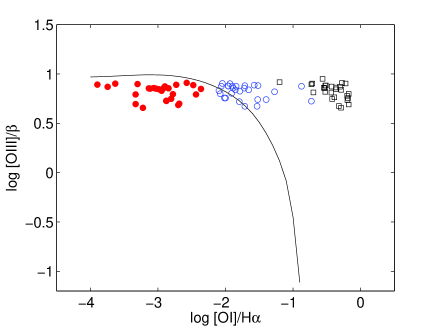
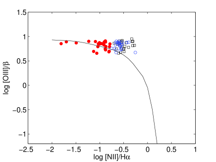
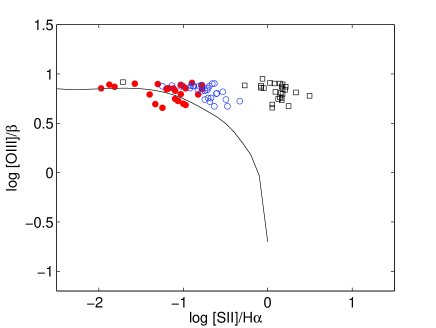
In Fig. 3 we compare the modelling results with the Kewley et al (2001) diagnostics. [OI], [NII] and [SII] lines were not observed, so we use the results of models which better fit the observed line ratios. We adopt O/H solar, N/H =0.3 solar and S/H solar (Contini 2015, table 1). Fig. 3 top diagram shows that SB models are definitively in the SB zone, AGN models in the AGN zone, even if some models calculated for AGN galaxies in the outflow case, are on the border line. For the other two diagrams ([OIII]/H${\beta}$ vs [NII]/H${\alpha}$ and [OIII]/H${\beta}$ vs [SII]/H${\alpha}$ ) most of the SB models are on the border line. This already suggests that some galaxies show a complex character of SB and AGN. The spread of the [OI]/H${\alpha}$ line ratios and, in particular, the separation between the inflow from the outflow results, is due to the geometrical thickness large range of the emitting clouds in the AGN dominated models. In the outflow case (Fig. 1), the clouds may contain in the internal region, between the shock front edge and the edge illuminated by the AGN flux, a low temperature zone with large quantities of gas in the physical conditions suitable to the [OI] line. The same could explain the spread of the [SII] lines. However, when referring to the data instead of to the models, the S/H relative abundance also changes from object to object because S is easily trapped into dust grains. The [NII]/H${\alpha}$ line ratios fill a more compact region throughout the diagram and the AGN inflow and outflow models overlap, because the region throughout the cloud where N⁺ prevails is radiation dominated. We have found by detailed modelling of different types of spectra emitted from galaxies at 0.01$\leq$z$\leq$3 that N/H varies within a factor of 10 throughout all the z range (Contini 2016, fig. 5). So inserting eventual observation data instead of model results in Fig. 2 middle diagram, the picture would change.

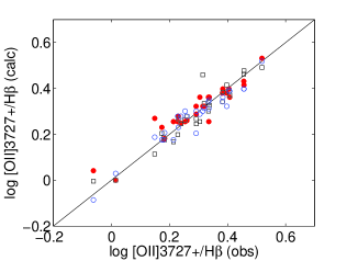
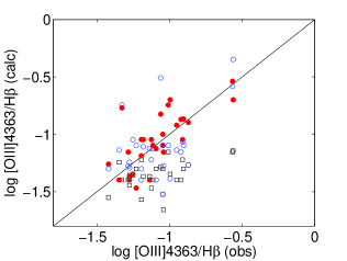
In Fig. 4 we check the modelling result precision. The observational uncertainties are not shown for sake of clarity. The [OIII] 5007+/H${\beta}$ and [OII]3727+/H${\beta}$ calculated line ratios reproduce satisfactorily the data, indicating that the physical conditions and the relative abundances, adopted in the calculations of the spectra, are sound. The same models were used to calculate for each object the [OIII]4363/H${\beta}$ line ratios shown in Fig. 4, right diagram. The observed [OIII]4363 lines are rather weak. Even accepting discrepancies by a factor of 2, Fig. 4 (right diagram) indicates that several models referring to the AGN outflow case should be dropped.

4 Discussion and concluding remarks

4.1 Physical conditions, metallicities and SFR in the sample galaxies

Figure 4: Left : observed vs calculated [OII]3727+/H${\beta}$ . Middle :observed vs calculated [OIII]5007+/H${\beta}$ . Right : observed vs calculated [OIII]4363/H${\beta}$ for single galaxies. Symbols as in Fig. 3.

Figure 5: Top panel: calculated H${\beta}$ in $\rm erg\,cm^{-2}\,s^{-1}$. Symbols as in Fig. 4 Bottom panel : the SFR in M_⊙ yr^-1 given by Ly et al.

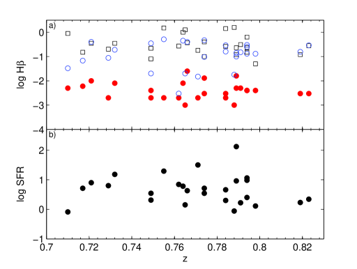
Tables 2-4 show that $\rm V_{s}$ $\sim$ 100 $\rm km\,s^{-1}$and $\rm n_{0}$ $\sim$ 200 $\rm cm^{-3}$ in most of the galaxies characterize the gaseous clouds in the SB environment, while preshock densities are higher by a factor of 1.5-10 in the AGN clouds. The SB clouds show major fragmentation ($D$ $\sim$ 10¹⁶ cm). In the AGN, $D$ ranges from 10¹⁶ cm to a maximum of $>$10 pc for the ejected clouds. Geometrical thick clouds up to D=3 pc were calculated for the merger galaxy NGC 6240 (Contini 2012b). Combining an average H${\beta}$ flux of 10^-16 $\rm erg\,cm^{-2}\,s^{-1}$observed at Earth (Table 1) with an average H${\beta}$ flux calculated at the nebulae (Table 4) for the SB clouds ($\sim$0.01 $\rm erg\,cm^{-2}\,s^{-1}$) and for the clouds in the AGN environment ($\sim$0.1 $\rm erg\,cm^{-2}\,s^{-1}$), we obtain the average distance of the emitting clouds from the SB R_SB$\sim$ 0.5 kpc and from the AGN R_AGN$\sim$ 0.16 kpc, respectively, adopting a filling factor $\sim$1. The starburst effective temperatures $\rm T_{*}$ are similar to those found in quiescent galaxies (4-7 10⁴ K, Contini 2014b).

Metallicities, in term of the O/H relative abundances, are a crucial issue for galaxies at high z. The O/H relative abundances calculated by detailed modelling are about solar (6.6 10^-4, Allen 1976) for all the objects, except for a few AGN with O/H= 0.3 -0.5 solar. Ly et al (2015) obtain 0.223-3.23 10^-4 by the T_e based metallicity determination (cf. Contini 2014a). The discrepancies between metallicity results obtained by different modelling methods are explained in Sect. 2.

In Fig. 5 the H${\beta}$ absolute fluxes (in $\rm erg\,cm^{-2}\,s^{-1}$) calculated at the emitting nebula and the SFR (in M_⊙ yr^-1) given by Ly et al. are shown as function of the redshift. Throughout a small z range, they do not show any trend, while (Contini 2016, fig. 6 and references therein) SFR in SN and GRB host galaxies were found to increase with z on a large scale for z$\geq$0.1. At lower z, SFR do not show any particular slope. On the other hand, SFR presented by Ramos Almeida et al (2013) for X-ray and mid-infrared selected galaxies at 0.4$\leq$z$\leq$1.15 exhibit an increasing trend. More objects should be considered. Moreover, SFR $\propto$ L(H${\alpha}$ )_Earth (the H${\alpha}$ luminosity observed at Earth) and L(H${\alpha}$ )_Earth = L(H${\alpha}$ )_nebula (the H${\alpha}$ luminosity calculated at the nebula) which is $\propto$ H${\alpha}$ R². We adopt H${\alpha}$ /H${\beta}$ $\sim$3. R is the distance of the emitting cloud from the radiation source. So SFR $\propto$ H${\beta}$ , assuming an average R. Ly et al results show that SFR in AGN and SB galaxies are very similar, whereas from the H${\beta}$ flux calculated at the nebulae (Fig. 5, top diagram), higher SFR for AGN are expected. This discrepancy can be explained by the coexistence of AGN and SB in most of the sample objects.

Figure 6: Observed vs calculated R_[OIII] (left) and [OII]3727+/[OIII]4363 (right) for single galaxies. ID numbers (see Table 1).

Table 5: Galaxy types resulting from the modelling

1	2	3	4	5	6	7	8	9	10	11	12	13	14	15	16	17	18	19	20	21	22	23	24	25	26	27	28
S	S	S	S	S	-	-	S	-	S	S	S	S	S	S	S	S	S	S	S	S	S	-	-	S	S	S	S
-	-	1	-	-	1	1	-	-	-	-	-	-	-	1	-	1	-	1	-	-	-	1	-	-	-	-	-
-	-	-	0	-	-	-	0	0	0	-	0	0	0	-	-	0	0	-	-	-	0	0	0	-	0	-	-

4.2 Multiple radiation sources in single galaxies

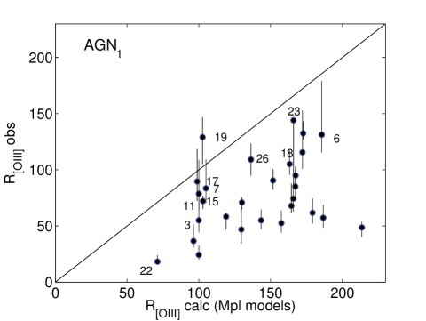
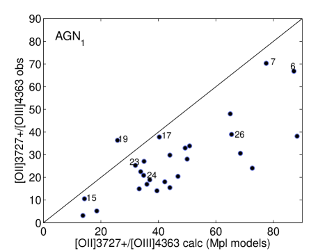
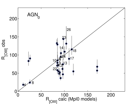
By AGN and SB dominated models, we reproduced successfully the [OIII]5007+/H${\beta}$ and [OII]/H${\beta}$ observed line ratios, not always the [OIII]4363/H${\beta}$ from each galaxy. We investigate whether the photoionization source in each object is an AGN, a SB or both, comparing in Fig. 6 left diagrams and right diagrams, the calculated with observed corrected R_[OIII] and [OII]/[OIII]4363, respectively. The top diagrams refer to results obtained by SB dominated models, the middle ones by AGN dominated models with outflowing clouds and the bottom diagrams show the results of models dominated by AGNs which accrete the surrounding clouds. Fig. 6 shows that models MSB1-MSB28 (Table 2) reproduce the data within the observational errors, except for ID 6, 7, 23 and 24 (Fig. 6 top diagram). Most of the Mpl1-Mpl28 model results (Table 3) overpredict the data, except ID 19 (Fig. 6 , middle). ID 3, 6, 7, 15, 17, 19 and 23 R_[OIII] are reproduced within $\sim$ 30%. Fig. 6 bottom diagram refers to models Mpl01-Mpl028 (Table 4). About half of the object spectra are well reproduced by the AGN accretion models. The results show that some line ratios can be explained with the same precision by both the SB and AGN dominated models. The galaxy types are schematically shown in Table 5 (S=SB, 1=AGN₁, 0=AGN₀), where AGN₁ refer to ejection of matter outwards and AGN₀ to accretion.

Summarizing, calculation results suggest that most of the objects contain a SB, about 5 objects are AGNs. Half of the galaxies show multiple radiation sources : a SB + an accreting AGN. ID 3, 15, 17 and 19 show an SB + an AGN with outflowing matter. ID 17 and ID 23 host a double AGN, but ID 17 also a SB. The AGNs show gas accretion rather than outflow, suggesting an AGN-SB correspondence. Multiple nuclei are found in local galaxies which derive from merging, e.g. in Arp 200 at z=0.018 (Graham et al 1990), where O/H relative abundances are about solar and N/H are higher than solar by a factor of $\sim$1.5 throughout the starburst region (Contini 2013). To complete our investigation we need measurements of the [OI], H$\alpha$, [NII] and [SII] emission lines, which are only available with near-infrared spectroscopy at z$\sim$0.8.

References

Allen, C.W. 1976 Astrophysical Quantities, London: Athlone (3rd edition)

Anders, E., Grevesse, N. 1989, Geochimica et Cosmochimica Acta, 53, 197

Asplund, M., Grevesse, N., Sauval, A.J., Scott, P. 2009, ARAA, 47, 481

Blank, M. , Duschl, W.J. 2014, IAUS, 303, 379

Contini, M. 2016, MNRAS, in press (ArXiv:1605,02438)

Contini, M. 2015, MNRAS, 452,3795

Contini, M. 2014b, A&A, 572, 65

Contini, M. 2014a, A&A, 564, 19

Contini, M. 2013, MNRAS, 429, 242

Contini, M., Contini, T. 2007, AN, 328, 953

Contini, M., Aldrovandi, S.M.V. 1986, A&A, 168, 41

Dixon, T.G., Joseph, R.D. 2011, ApJ, 740, 99

Engel, H. et al. 2010, A&A, 524 ,56

Graham G. R., Carico D. P., Matthews K., Neugebauer G., Soifer B. T., Wilson T. D. 1990, ApJ, 354, L5.

Hopkins, P.F. , Quataert, E., Murray, N. 2011, MNRAS, 417, 950

Kewley, L.J., Dopita, M.A., Sutherland, R.S., Heisler, C.A., Trevena, J. 2001, ApJ, 556, 121

Ly, C., Rigby, J.R., Cooper, M., Yan, R. 2015, ApJ, 805, 45

Osterbrock, D.E. 1974 in ’Astrophysics of Gaseous Nebulae’ W.H. Freeman and Company, San Francisco

Ramos Almeida, C., Rodríguez Espinosa, J. M., Acosta-Pulido, J. A., Alonso-Herrero, A., Pérez García, A. M., Rodríguez-Eugenio, N. 2013, MNRAS, 429, 3449

Zubovas, K., Nayakshin, S., King, A., Wilkinson, M. et al 2013, MNRAS, 433, 3079