Store Location Selection via Mining Search Query Logs of Baidu Maps
Abstract
Choosing a good location when opening a new store is crucial for the future success of a business. Traditional methods include offline manual survey, which is very time consuming, and analytic models based on census data, which are unable to adapt to the dynamic market. The rapid increase of the availability of big data from various types of mobile devices, such as online query data and offline positioning data, provides us with the possibility to develop automatic and accurate data-driven prediction models for business store placement. In this paper, we propose a Demand Distribution Driven Store Placement (D3SP) framework for business store placement by mining search query data from Baidu Maps. D3SP first detects the spatial-temporal distributions of customer demands on different business services via query data from Baidu Maps, the largest online map search engine in China, and detects the gaps between demand and supply. Then we determine candidate locations via clustering such gaps. In the final stage, we solve the location optimization problem by predicting and ranking the number of customers. We not only deploy supervised regression models to predict the number of customers, but also learn to rank models to directly rank the locations. We evaluate our framework on various types of businesses in real-world cases, and the experiments results demonstrate the effectiveness of our methods. D3SP as the core function for store placement has already been implemented as a core component of our business analytics platform and could be potentially used by chain store merchants on Baidu Nuomi.
keywords:
Business; Store placement; Multi-source data; Machine learning1 Introduction
Selecting a location when opening a new store is crucial for future business development: a good location may lead to very good business, while an incorrect one may result in serious business risk and even the failure of business.
Many efforts have been made to address this task both qualitatively and quantitatively. For example, one can conduct offline manual survey on one potential location. And many business consulting companies provide consulting services by collecting and mining data from third parties such as census and demographic data from the government. Some previous work [2, 25, 5] study optimal location problem as a covering problem which maximizes the number of people a location can attract.
Nowadays, personal mobile devices are ubiquitous with large scale mobile data, making it possible for us to offer big data driven solutions for business solutions, especially for business location selection in our topic here. In a recent work [14], the authors have developed a data-driven approach to solve the problem of retail store placement by predicting the check-in numbers at given locations using linear supervised learning model. However, these models do not capture the targeted user demands (i.e., demands for a category of stores).
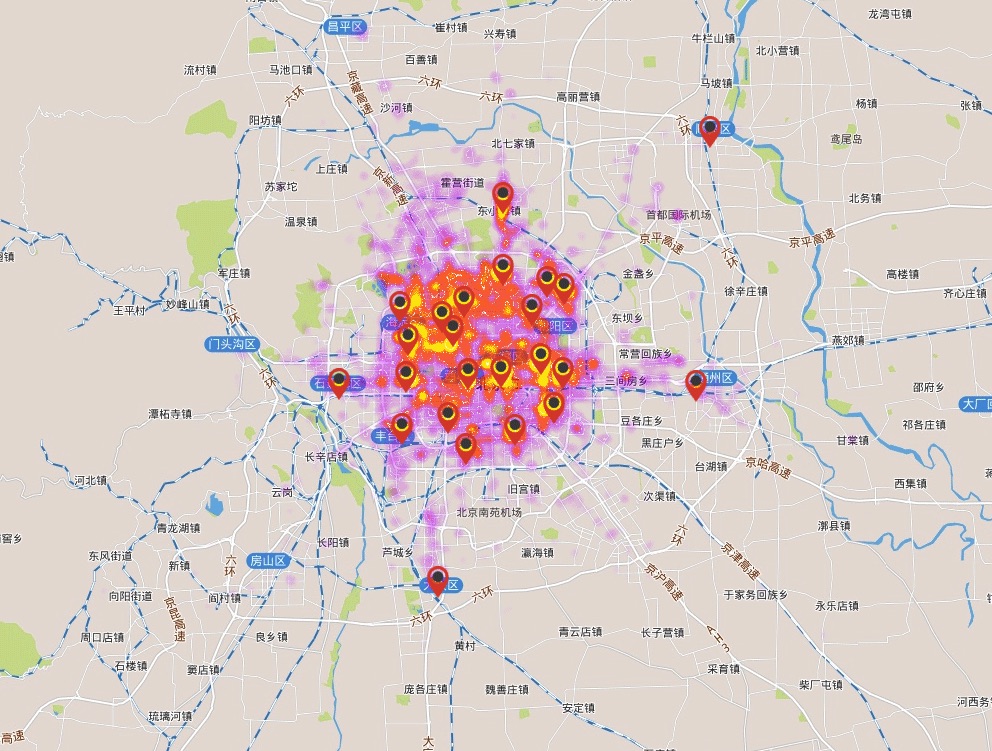
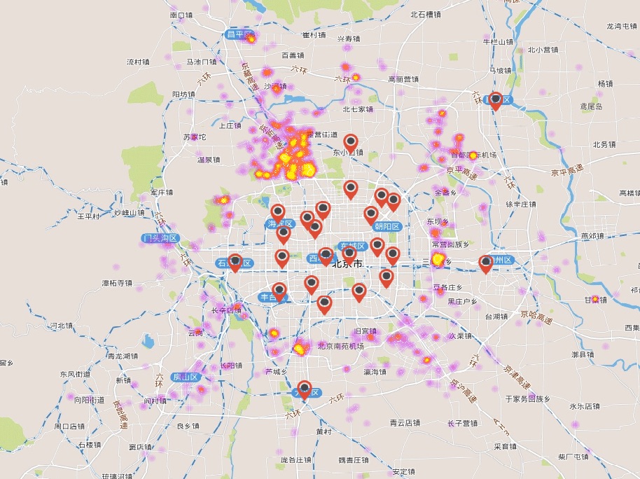
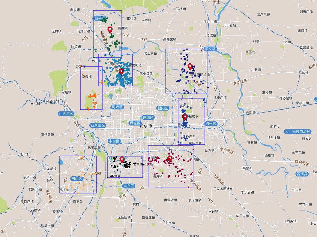
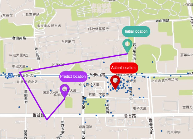
In this paper, we propose a Demand Distribution Driven Store Placement(D3SP) framework, and utilize multiple spatial-temporal data sources to accomplish this task. Given the category of a new store to be opened, the aim of our approach is to identify several most promising locations that meet user demands and attract a large number of potential customers. In this paper, we take advantage of search query data from Baidu Maps and integrate other types of spatial-temporal data sources such as POI data etc to solve the problem.
Location based applications like map search and navigation systems have been developed in recent years. The will of users going to some places can be inferred from this kind of data (i.e., map query data), demonstrating the potential consumptive demands of users [24]. Generally, the strategy of finding optimal placement is to find the most suitable locations from a list of candidate locations [23]. Here, we define those candidate locations as the places where demands exceed supplies. An example of finding optimal placement for opening a new “Haidilao” using D3SP is shown in Figure 1. For example, when users query “Haidilao” (a popular hot pot restaurant in China), their locations are recorded. In Figure 1(b), after excluding the locations within 5km around the existing stores, there are still many places that do not meet user demands. It is possible to cluster the gaps between demand and supply (Figure 1(c)), and then optimize the placement to obtain most customers (Figure 1(d)).
Location placement is naturally a ranking problem. There are at least two methods to achieve. We can first predict the customer numbers and then rank manually, or utilize learn to rank methods directly. In this paper, we will try both and evaluate the results with real-world cases. A lot of factors can impact the number of customers a location can attract. We consider economic development, popularity and transportation convenience [22] in our model. The models are trained and validated with existing stores’ locations and customers’ behavior.
Our work makes the following contributions:
-
•
First, we identify the spatial distribution of user demands from map query data, and obtain the places that demands exceed supplies. Here, we extracted two types of demands of real users: specific demands (for specific brand of chain store) and general demands (for a general category) from the data.
-
•
Second, we propose practical features and models to rank the candidate locations. We utilize both supervised regression models to predict the number of customers, and learn-to-rank models to rank the candidate locations directly. Novel features such as distance to the center of the city, popularity of specific area category and real estate price nearby are also proposed.
-
•
Finally, we evaluate our methods with real-world cases, and developed a completed system to find optimal placement for opening a new store. D3SP is a crucial part of the location-based business support system developed in Baidu. We evaluate D3SP on both experiments and the real cases. The experiments show that our framework predicts accurately for various categories, and the real cases show that our framework works well in the real world.
2 Data and Framework
2.1 Data and Preprocessing
In this section, we provide details of the heterogeneous data sets we use in this paper, as well as the preprocessing of these data sets. The data sets include map query data, POI data and WiFi Connection data.
Location query data from Baidu Maps. Map query data contains over one billion queries from 500 million users using Baidu Maps on mobile phones. Each map query record has the following information: an anonymized user ID, timestamp, latitude and longitude of the location where the query was issued, query keywords with the associated POI attributes.
When a user searches for a place or navigates a route to a place using Baidu Maps, the query action reflects a demand of a specific place or a category. The actual location where the user issues a query also implies a spatial demand. For example, a query [, 2015-08-08 08:42:28, (116.34, 40.02), “Starbucks”] means that the user wants to have coffee at location (116.34, 40.02). Further analysis can be found in Section 3.
POI data. Point-of-Interest(POI) in a city is tightly related to people’s consumptive behavior. We can learn a lot from existing POIs that are similar to a new store to be opened. The POI data set is a collection of POIs. For each POI , its attributes include POI ID , location , or and , category and other detailed information. Attribute “category” has two hierarchical levels. For example, category “hotel” is the upper level, and “express inn” is the subcategory of “hotel”.
WiFi Connection data. We obtained WiFi Connection data from a third-party data source, which contains records of 3-month historical WiFi connections from June 1, 2015 to August 30, 2015. Each record contains an anonymized user id, timestamp, and the corresponding POI.
WiFi Connection data can be a good indicator of customer numbers, and serves as part of ground truth in prediction of customer numbers. It has several advantages over the check-in data used in previous work [14]. First, only the customers can connect the WiFi in the POI, which eliminates the situation of cheated check-ins. Meanwhile, WiFi Connection data has usually many more records than the check-in data for a single user. A user often connects to wifi in restaurants or hotels, but does not necessarily check in her locations.
Integrating the data sets. By integrating WiFi Connection and POI, we obtain the total number of customers for each POI. Note that each user can generate several records in one day at a specific POI, and some POI may have several accessing points. However, for a POI, the number of customers in one day should be the appearance of all the users in that day. Therefore, we clean the data by maintaining one record for a user in one day at a specific POI. Each record contains a POI id, POI category, POI name, POI location and POI customer number. In further analysis, we use the POI customer number to measure how good a store location is.
Data privacy. In this paper we were very careful to protect the user privacy. We have set several key steps and protocols to protect the privacy:
-
•
First, all ids in our data are hashed and anonymous. None can be linked to any real-world identifier of a person. So we do not know the offline behavior of any real person.
-
•
Second, we have a very strict agreement with the third party that the WiFi Connection data is kept secure, safe and anonymous. Each id is encrypted, and is not even linkable to the ids in map query data.
-
•
Finally, we are focused on analysis in aggregation level. For example, we aim to predict the number of customers of a location as a whole, instead of predicting whether a specific user will visit. None individual level analysis is deployed in our paper.
2.2 Framework and methodology
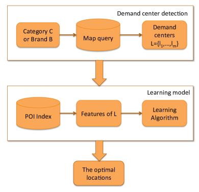
A promising location for a new store has two requirements. First, it should meet users’ demands while there are not too many competitions. Second, it needs to attract a significant number of customers. In this paper, we aim to first figure out a few candidate locations by detecting demand centers, and then rank them by predicting the custom number that each location may have. Figure 2 shows the overall framework of our paper, and more details are as follows.
In a city, there can be many locations to choose for opening a store. Our first step is to find several demand centers as candidate locations for a store category or a specific brand of chain stores . Map query data is used to find the demand points where the users query a POI or a POI belonging to the same category. Thus, we obtain the demand centers from those locations.
Then, we transform the problem into a global ranking problem. Our goal is to rank the locations in for opening a new store belonging to category. we achieve this by predicting the customer number for each location in . Here we train a supervised machine learning model with the customer numbers of existing stores. The features are mined from an area . Here is a disc centered at with radius . Considering users’ walking distance and GPS position shifting, we set to be 1 km. With this model, we are able to predict the custom numbers of the candidate demand centers will have. Locations with higher values are more desirable to open new stores.
3 Obtaining demand centers
Our work is inspired by the fact that map queries reflect users’ targeted demands. Each query contains a source place and a destination. The source place has demands while the destinations can supply the demands. An ideal place for a new store to be opened is where there are many demands but few supplies. In this section, we aim to identify such places with the knowledge of map query data. We start from the analysis of user demands, and then propose methods to identify the demand centers.
3.1 User Demand Analysis

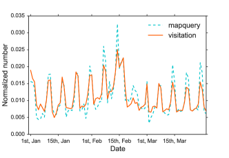
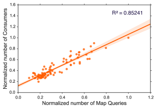
An important part of our method is the modeling of user demands. We will first demonstrate that map query reflects user demands, and it is highly correlated with users’ real visitation. We analyze the percentage of the query sessions which users actually go to that place over all the query sessions. We utilize the method in [24] which assumes that a queried location is actually visited by the user if there is at least one location record in user’s next 1.5-day mobility trace, and the distance of the location record and the queried location is less than 1 km. As shown in Figure 3, the normalized number of map query and real visitations have similar dynamic patterns in a three months period. In Figure 3(b) we also plot the coefficient of determination . The numbers of map queries and real visitations have a correlation up to 0.85. These results confirm that map queries are highly correlated with real visitations, and the number of map queries can be indicators of customer numbers and real user demands. More specifically, the visitation ratio can reach the ratio nearly 50%, which is also a strong evidence that there is a relationship between map queries and user demands.
Next, we will further analyze user demands via map query data. Remind that a map query record has the following attributes: timestamp , latitude and longitude of the location where the query was issued, query keyword, attributes of POI. Formally, we denote a demand point as . That is, a demand point contains the locations and a timestamp where and when the demand happens. We extracted two types of demands of real users. The first type is specific demands. This type of demands can be extracted from the route data in Baidu Maps. For example, a user has a specific need that he wants to get to Starbucks. He or she searches for the routes from his or her current location to a store of Starbucks at time . This implies that the user has a specific demand on Starbucks. Another type of demands are general demands. An example is that a user has a general demand that he wants to drink some coffee, but he does not have preference on brands. This type of demands can be extracted from the “nearby” queries which return POIs nearby according to the keyword.
After we define both specific and general demands, we conduct analysis on the demand points we extract from queries. Our analysis basically identifies the temporal and spatial differences among different queries. Here we take Starbucks and Haidilao (a popular hotpot restaurant in China) as examples.
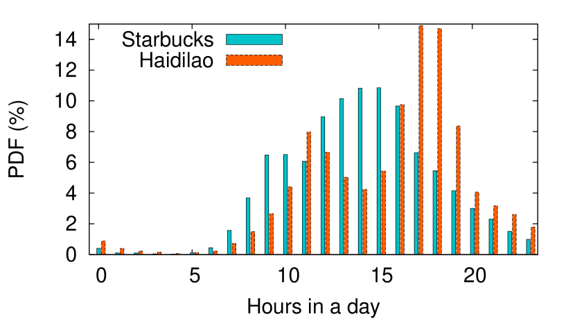
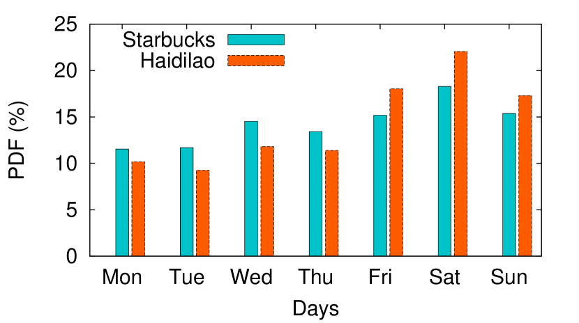
Active time. In Figure 6 and 6 we plot the active time of the demand points. We find different demands are active at different time. For example, people usually get to Starbucks during the day, while they go to Haidilao at noon and evening for meals. In a week, people prefer to go to Haidilao on Friday, Saturday and Sunday, while people do not show obvious preference on Starbucks.
Effective distance. We also realize that people may tolerate different distances for different stores. In Figure 6, we plot the distribution of distance between source and destination. While 80% queries of Starbucks are within 2 km, up to 40% queries of Haidilao are more than 5 km. This is understandable, since few people will travel 5 km just for a coffee. Therefore, the nearby area of the location where the user makes a query can be seen as a place where the user demand for the queried place.
The above analysis reveals that user demands may have various features and patterns. When we further detect the demand centers, we need to take the type of demands into consideration.
3.2 Finding Demand centers
To find demand centers, we have three steps: identifying demand points, excluding supplies, and clustering demands.
Identify demand points. In the first step, we will identify and characterize the demands, e.g., Starbucks. As we explain before, we extract timestamp and location from each query, including specific demands with targeted keywords Starbucks or general demands with categories or tags of coffee from “nearby” queries. We then characterize the temporal and spatial features of demands.
Exclude supplies. After we identify the geographic distribution of demand points, we need to identify the gap between demands and supplies. For specific demands, we directly exclude areas where there are already supplies. Here the exclusion is based on distance features. From the distribution of source and destination distance, we identify a threshold of 80%, i.e. 80% of users will not get to a store farther from corresponding distance. Then for each existing store, we consider demand points within the threshold are supplied. Thus these demand points are excluded. The remaining demand points are the demand-supply gap points where demands exceed supplies. For example in Figure 6, 80% of the users search “Starbucks” are within distance 2km. The demand points within 2km from the existing stores are excluded.
For general demands, we exclude supplies with some probabilities, because the user has the potential to a new store. We calculate the distance between the nearest existing store and the demand location of user . Also the number of existing stores nearby is defined as . For a user , if is large, the probability of the demand to be satisfied is low. On the other hand, if is large, the probability is high. Therefore, we define two scores according to the two intuitions. One is the distance score , another is the supply score . The score of a demand to be remained . Here we set , and . Figure 7(a) shows the demand points of coffee shops and existing stores in an area. Figure 7(b) shows the remaining demand points after we remove the possible satisfied ones. We can see that the demand points near the existng stores are more likely to be excluded.
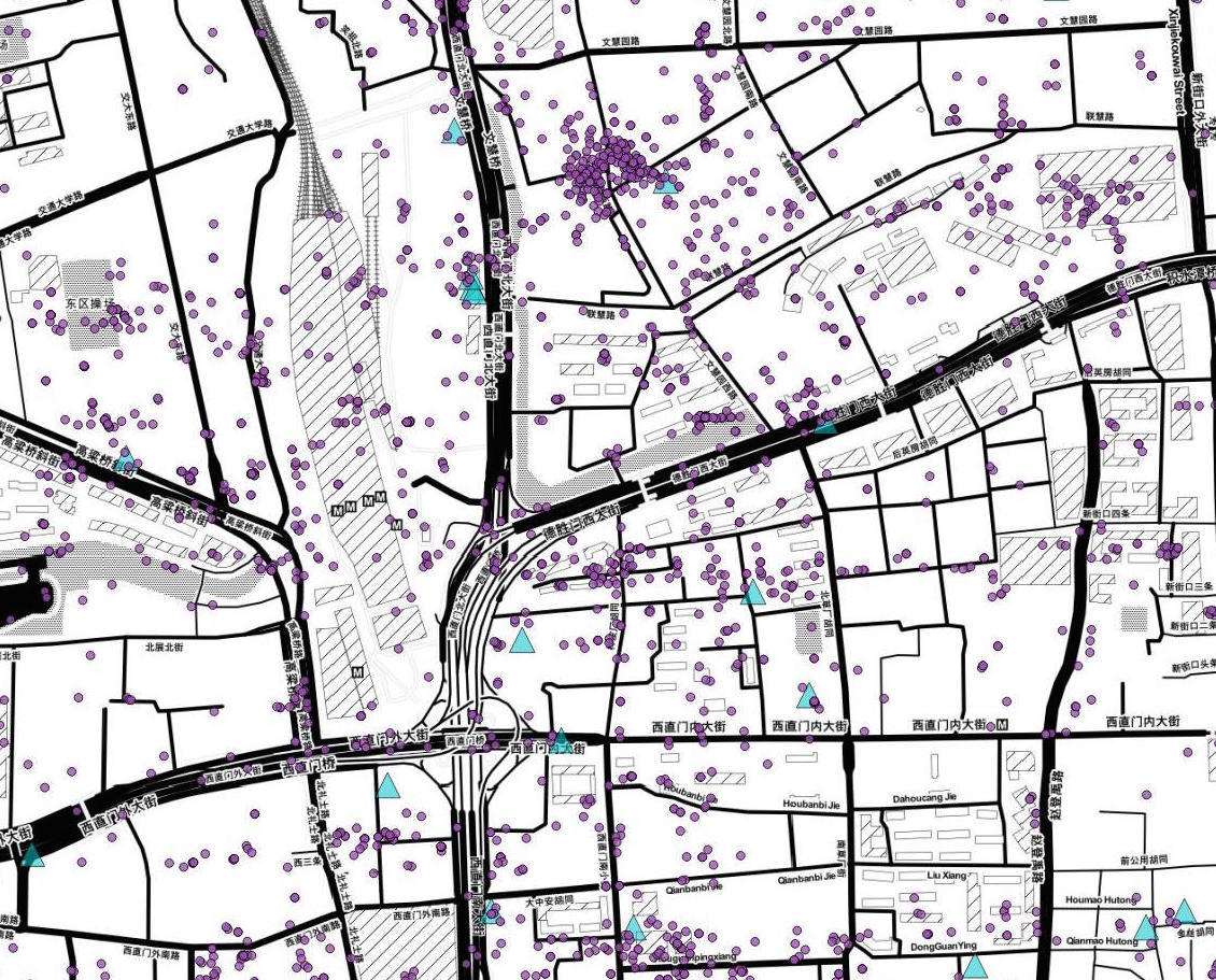
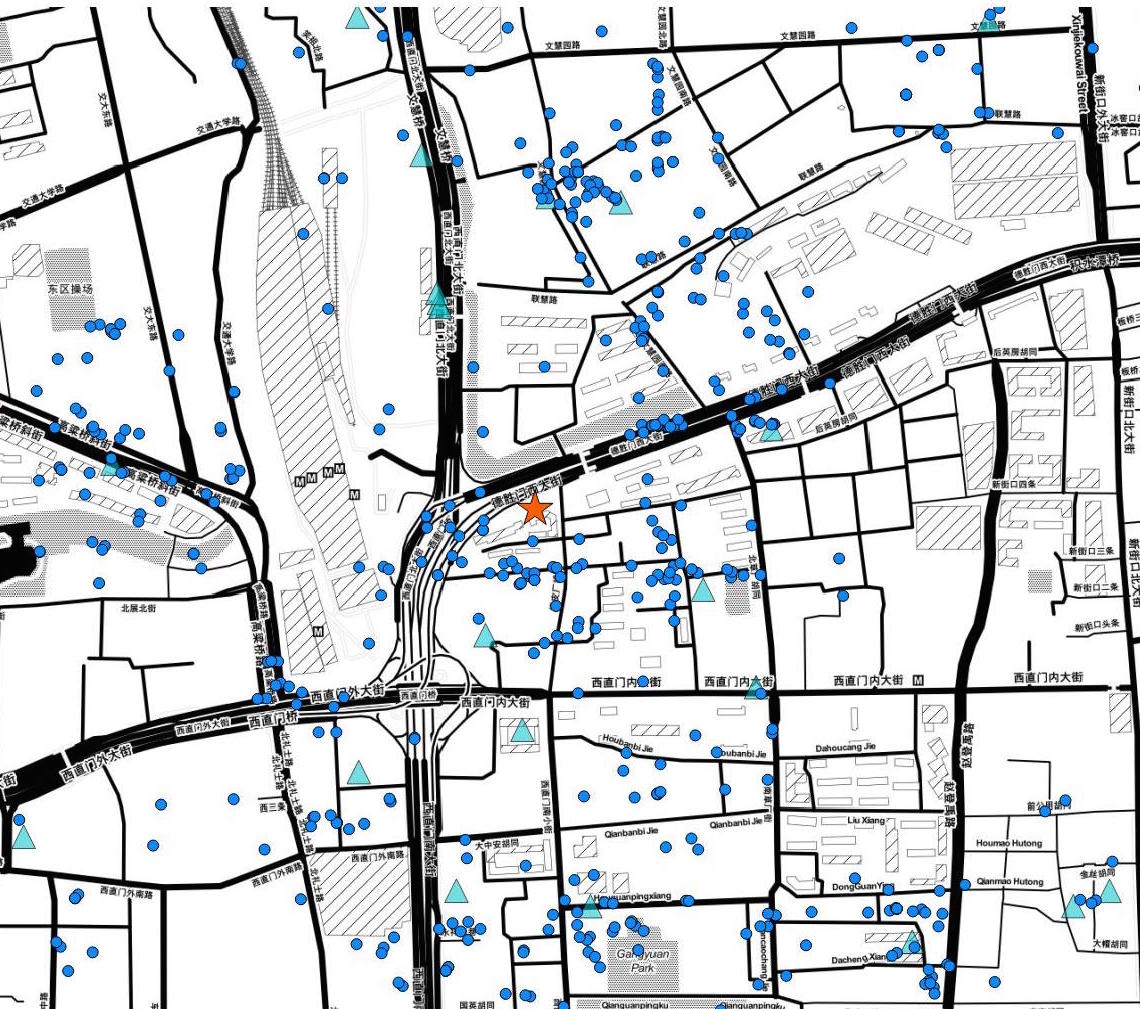
Clustering demands. After we identify the demand-supply gap points, obtaining a place for a new store is still not trivial. This is because the demand points are placed in space without any regularized shapes. Here, we leverage machine learning clustering algorithms, and select the cluster centers. Since we do not know the exact number of clusters we will have, and would require a center point of each cluster, we use MeanShift [6] as our algorithm. We set the bandwidth parameter as the distance threshold we identify in the previous step. This algorithm automatically clusters the demand-supply gap points and returns a center for each cluster. we denote the center points as demand centers which are candidate locations for store placement. The star in Figure 7(b) is the demand center we find.
4 Ranking promising locations
With the demand centers, we next rank these promising locations. In this paper we utilize supervised machine learning models to rank the locations. There are two directions. First, we can directly apply learn-to-rank methods. Second, we can predict the number of customers with regression models, and then rank based on the predicted customer numbers. We consider both in our paper, as illustrated in Sec 4.1. Then we will introduce the features we use in our models.
4.1 Ranking Algorithms
Given a list of demand centers , we utilize the supervised learning methods to rank or predict the number of consumers of a new store located at . The locations with higher scores are the optimal placements.
Baseline. The baseline method is to rank randomly, and the locations rank at top are the results.
Learn to rank. We first directly apply learn to rank methods. The method we use in this paper is LambdaMART [4], which is a widely used learn to rank method in many works and the winner of 2010 Yahoo! Learning To Rank Challenge. It is a combination of boosted tree MART and a learn to rank method LambdaRank.
Regression. For regression method, we consider the linear regression with regularization (Lasso) and the kernel methods including Support Vector Regression (SVR) [10] and Kernel ridge regression (KRR) [18]. We also consider two ensemble methods Random Forests (RF) and Gradient Boosting Decision Tree (GBDT).
Mathematically, Lasso consists of a linear model trained with L1 prior as regularizer. The objective function to minimize is:
| (1) |
where is feature vectors and is the target score. is a constant and is the -norm of the parameter vector.
In SVR, training vectors are implicitly mapped into a higher (maybe infinite) dimensional space by the kernel function. KRR combines Ridge Regression (linear least squares with l2-norm regularization) with the kernel trick. It thus learns a linear function in the space induced by the respective kernel and the data. For non-linear kernels, this corresponds to a non-linear function in the original space.
Random Forests[3] and Gradient Boosting Decision Trees[7] are two popular algorithms of the ensemble method. Random Forests is a notion of the general technique of random decision forests. It constructs a multitude of decision trees at training time, and outputs the class that is the mean prediction of the individual tree. Each tree in the ensemble is built from a sample drawn with replacement from the training set.
Gradient Boosting is typically used with decision trees of a fixed size as base learners. For this special case Friedman proposes a modification to Gradient Boosting method which improves the quality of fit of each base learner.
4.2 Features
In this part, we will introduce the features mined from the multi-source data. Those features can reflect the quality of the area for the new store including functionality, transportation convenience, competition, economic development and so on. When given a location and the category of the new store to be opened, the features can be mined from the integrative dataset which is indexed in the geographic POI index. Remind that the Area around is which is a disc centered at with radius (1 km).
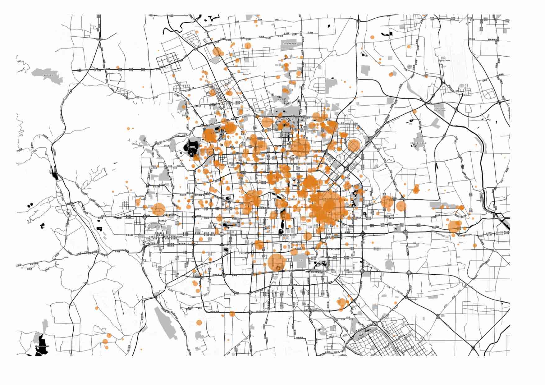
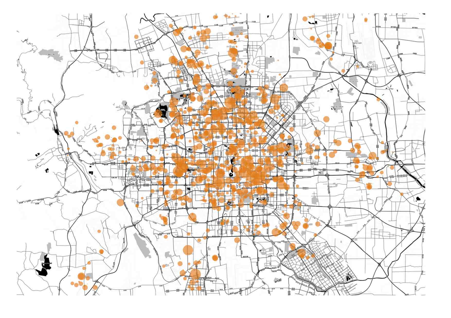
Distance to the center of the city. The popularity of a store is not only related with the local information about the location, but also related with its geographic position in a city. To see how the customers distribute for a kind of stores in a city, we draw the heat maps of the consumption behaviors for express inns and coffee shops in Beijing, respectively in Figure 8. The hotter(red color) the color of a point is, the more customers there are. We find locations near the center of a city usually attract more customers.
From the geographic aspect, we consider the distance between the location and the center of the city (here we consider the city of Beijing and the center is ).
| (2) |
We can see from the data analysis that the distance of a location to the center of city influences the popularity.
Traffic convenience. Here, we use the number of transportation stations(including bus stations and subway stations) in to denote the traffic convenience.
| (3) |
is the set of transportation stations in Beijing.
POI density. Since the area of each for is the same, the number of POIs in is used to present the density of which is defined as
| (4) |
where P is the set of all POIs in a city.
Popularity of specific area category. We use the category of most POIs in to define the area category . The set of all the POIs of category C is defined as . Then, the popularity of specific area category is the average number of WiFi consumers for a category over all POIs in and its area category is . Formally,
| (5) |
where and are the category and location of , and is the number of WiFi consumers of POI .
Competition. We also consider the competition between the stores belonging to the same category. We define the number of POIs belonging to category C in is , and the total number of POIs in is . Then the competition is defined as the ratio of and , which is
| (6) |
Area popularity. Also, the popularity of can influence the popularity of . The people consumed at places in are the potential consumers for a new store opened at . The popularity of an area is defined as
| (7) |
To avoid self-correlation of the data, we eliminate the connections of the test POI when we evaluate the performance.
Real estate price nearby. The real estate price of an area reflects the economic development of a location in the area. Thus, given a location , we compute the average price of the nearest 5 real estate in 2km to estimate the price.
5 Evaluation
Given a POI category or a specific brand, we first evaluate the performance of our prediction method using existing POIs belonging to the same category or brand. Then, we show some real cases of store placement using our framework.
5.1 Metrics
After we predict the scores for each POI, we obtain a ranked list of locations . The ranked list of locations based on the actual popularity (number of customers) of those POIs is also obtained from the POI-Customer dataset. The position of location in is denoted with .
In order to evaluate the ranking performance of our result, we utilize the nDCG@k (Normalized Discounted Cumulative Gain) metric [12] and the nSD@k (normalized symmetric difference) metric proposed in [16].
nDCG@k. Discounted cumulative gain (DCG) is a measure of ranking quality. DCG measures the usefulness, or gain, of an item based on its position in the result list. The gain is accumulated from the top of the result list to the bottom with the gain of each item discounted at lower ranks. The at a particular rank position is defined as
| (8) |
Sorting documents of the result list by relevance, also called Ideal DCG (IDCG) till p. The normalized discounted cumulative gain(nDCG), is computed as:
| (9) |
A relevance score for an instance is its relative position in the actual ranking , i.e., .
nSD@k The normalized symmetric difference metric provides an analysis of comparing two top-k lists. Given two top-k lists, and , the normalized symmetric difference metric is defined as:
| (10) |
value is denoted by nSD@k which is always between 0 and 1.
| Dataset | Size | Dataset | Size |
|---|---|---|---|
| Coffee shops1 | 1733 | Inn 1 | 1108 |
| Coffee shops2 | 1807 | Inn 2 | 1265 |
| Starbucks | 149 | Home-Inn | 235 |
| Costa | 75 | JinJiang | 57 |
5.2 Evaluation data and algorithms
We use two categories of stores which are express inns and coffee shops to evaluate the performance of our framework. For each category, the test data are two brands of stores, which is to eliminate the bias of ranking and to avoid overfitting. Specifically, for coffee shops, Starbucks and Costa are chosen as the test data, and for express inns, two famous brands in Beijing “Home-Inn” and “Jin Jiang Zhi Xing” are chosen. Also, the training data sets are all POI belonging to category “coffee shop” and “express inn” in Beijing except the POIs in test data. In detail, express inns exclude “Home-Inn” are in dataset “Inn 1” and those exclude “Jin Jiang Zhi Xing” are in dataset “Inn 2”. In the same way, “Coffee shops 1” and “Coffee shops 2” are the two training set that exclude “Starbucks” and “Costa”, respectively. The number of items of each evaluation set are shown in Table 1.
We have used the corresponding implementations that are public available through the Scikit-learn machine learning package [19]. The abbreviation of the evaluated algorithms and the best parameter setting after several experiments are listed below:
-
•
We use Linear to denote the linear regression algorithm Lasso, the regularization parameter here equals to .
-
•
KernelR is the abbreviation of Kernel Regression. The kernel function of the Kernel Regression we use here is radial basis function kernel (RBF), and the regularization parameter is set to be 0.1.
-
•
For SVR, the kernel function we use is also RBF. The penalty parameter of the error term is set to be 1.0, and the kernel coefficient is set to be 0.1.
-
•
RF is short for Random Forests. The number of trees is 10, the minimum number of samples required to split an internal node is set to be 2. The function to measure the quality of a split is mean square error.
-
•
For the Gradient Boosting for regression (GBR), the loss function to be optimized is least squares regression, and the number of boosting stages is 100.
-
•
The baseline algorithm is to randomly rank the list of test set. The accuracy result is the mean of 100 times experiments.
-
•
LambdaMART is a famous learn-to-rank algorithm. The number of boosting stages is 100, and the learning rate is 0.1, the minimum loss required to make a further partition is 1.0.
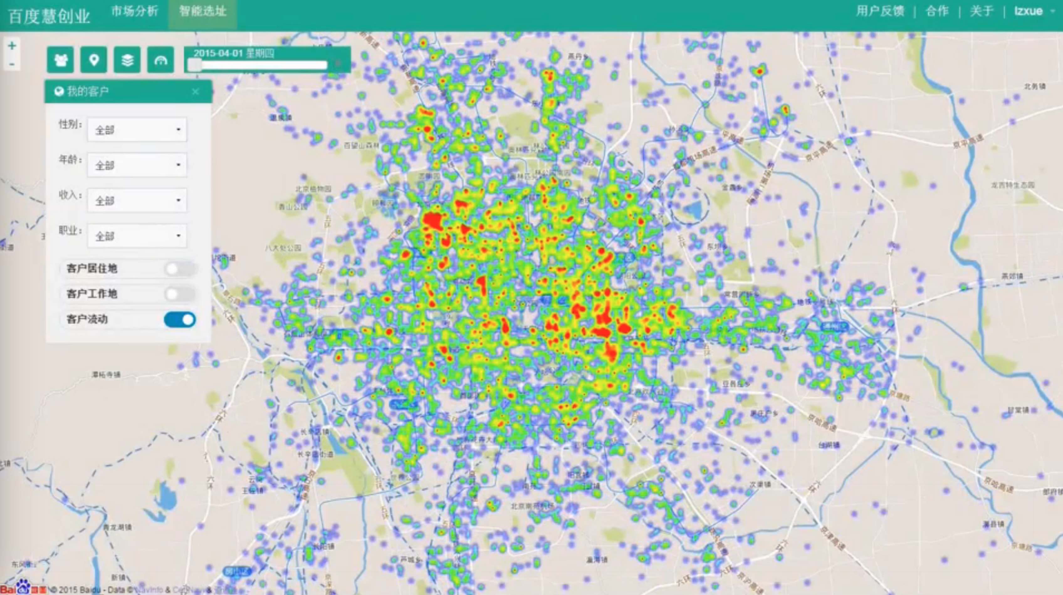
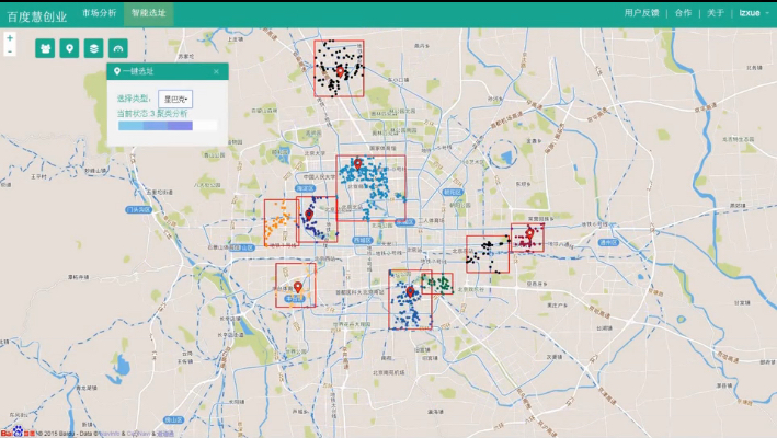
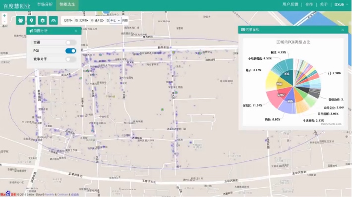
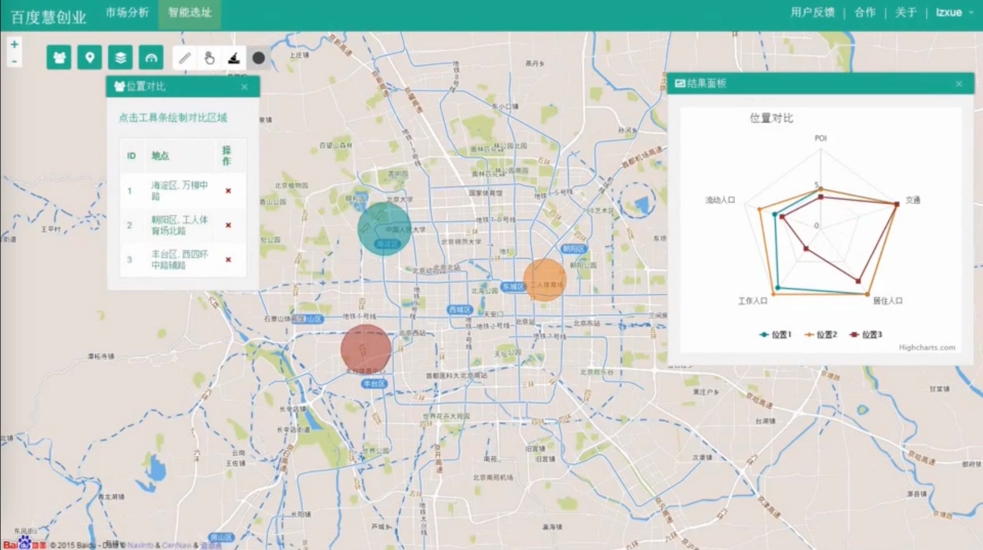
Also the implementation of system is shown in Figure 9. The whole system has four functions including detecting spatial distribution of different kinds of users, obtaining demand centers, location analysis and location comparison. Our framework D3SP covers two parts: obtaining demand centers and location analysis.
5.3 Feature importance
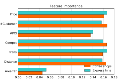
Before we show the results of prediction algorithms, we use Random Forests with the gini impurity to generate the feature importance for the two categories of POIs which is shown in 10. The features from top to down are the real estate price nearby, the popularity of the area, the number of POIs, the competition, the transportation, the distance to the center of the city and the category of an area. The feature importance of coffee shops and express inns are quite different. For coffee shops, the key features are the popularity of the area, the competition and the distance to the center. However, real estate price, competition and transportation are the key features for express inns. This is not surprising. The real estate price can influence the price of the express inns. When tourists choose a hotel, they tend to choose the one that is cheap and traffic convenient. Coffee shops usually attract people nearby. Competition exists everywhere and is important for all kinds of POIs. From the experimental results, we can see that the importance of features varies with the category of the store, and it’s necessary to learn from the stores belonging to the same category.
5.4 General demands accuracy
In this subsection, we evaluate the accuracy in the situation of general demands, and the categories are the coffee shops and express inns.
We first evaluate on the test sets in Beijing using the above two metrics with different learning methods. Evaluation results in Table 3 show that our results using learn-to-rank algorithm and ensembled methods are far more improved with respect to the random baseline method.
Accuracy with nDCG@10. We measure the performance of the algorithms trained on the features we extracted. As illustrated above, we know that the larger nDCG@10 is the more accuracy the result is. Table 3 show the accuracy results evaluated with nDCG@10 for both coffee shops and express inns.
With regard to the coffee shops, the best performance are using Random Forests and LambdaMART with nDCG@10 = 0.774 and nDCG@10=0.755 for “Starbucks” and “Costa”, respectively. The baseline results are nDCG@10 = 0.513 and nDCG@10 = 0.523. Not only Random Forests and LambdaMART, but also the other algorithms outperform the baseline algorithm. Learn-to-rank algorithm has larger nDCG@10 for the two test sets of express inns, whereas linear regression and baseline (randomly ranking) have lower nDCG@10. For example, in the “Home Inn” test, nDCG@10 for kernel regression, SVR, Random Forests, GBR and LambdaMART are 0.640, 0.680, 0.720, 0.685 and 0.736, respectively, while NDCG@10 of Linear Regression and Baseline are 0.510 and 0.540 which are less than the former ones. The JinJiang test shows the similar results, and the best accuracy is 0.767.
Accuracy with nSD@10. Unlike nDCG@10 evaluates the ranking of the lists, we use nSD@10 to evaluate the distance of two top-k lists which are the top-k real list and the top-k experimental list. Note that the smaller the nSD@10 is, the more similar the two top-k lists are. Table 3 also shows nSD@10 for both test sets of the two categories. As the result of coffee shops shown, the performances of Ensemble method algorithms are still better than the linear algorithm and the baseline algorithm. For “Starbucks” test, the baseline is 0.93, however, nSD@10 of Linear Regression, Kernel Regression, SVR, Random Forests, GBR and LamdaMART are 0.9, 0.9, 0.9, 0.6, 0.8 and 0.8. For “Costa” test, the baseline is 0.87, and the best result are Random Forests and LambdaMART with nSD@10= 0.6 which means that there are at least 4 predicted locations are in the top-10 of the real lists. Results show that the above conclusion is also similar for the express inns. The best nSD@10 for “Home Inn” and “JinJiang” are 0.8 and 0.7.
| Store | Algorithm | Measurement | |
|---|---|---|---|
| nDCG@5 | nSDK@5 | ||
| Starbucks | Linear | 0.530 | 0.85 |
| KR | 0.624 | 0.76 | |
| SVR | 0.683 | 0.67 | |
| RF | 0.740 | 0.56 | |
| GBR | 0.727 | 0.68 | |
| LambdaMART | 0.736 | 0.56 | |
| Baseline | 0.510 | 0.82 | |
| HomeInn | Linear | 0.555 | 0.872 |
| KR | 0.630 | 0.86 | |
| SVR | 0.687 | 0.75 | |
| RF | 0.715 | 0.65 | |
| GBR | 0.695 | 0.73 | |
| LambdaMART | 0.748 | 0.60 | |
| Baseline | 0.536 | 0.892 | |
5.5 Specific demands accuracy
Unlike general demands, for specific demands, we evaluate on two brands of chain coffee shops and chain express inns which are “Starbucks” and “Home Inn” using nDCG@5 and nSD@5. We randomly choose 20% of the data as test and remaining as training data. Table 2 shows the average results of the 10 times repeated experiments.
Comparing with the baseline 0.510, Random Forests is the optimal learning algorithm for “Starbucks” with nDCG@5=0.740 which offer about 45% improvement. For “HomeInn”, the optimal learning algorithm is LambdaMART with nDCG@5= 0.748. Also, the lowest nSD@5 are 0.56 and 0.65 for “Starbucks” and “Home Inn” respectively. Above results show that our framework also works well on the chain stores.
| Store | Algorithm | Measurement | Store | Algorithm | Measurement | ||
|---|---|---|---|---|---|---|---|
| nDCG@10 | nSDK@10 | nDCG@10 | nSDK@10 | ||||
| Starbucks | Linear | 0.560 | 0.90 | Home-Inn | Linear | 0.450 | 1.0 |
| KR | 0.740 | 0.90 | KR | 0.640 | 0.90 | ||
| SVR | 0.650 | 0.90 | SVR | 0.680 | 0.90 | ||
| RF | 0.774 | 0.60 | RF | 0.720 | 0.80 | ||
| GBR | 0.750 | 0.80 | GBR | 0.685 | 0.80 | ||
| LambdaMART | 0.766 | 0.80 | LambdaMART | 0.736 | 0.70 | ||
| Baseline | 0.513 | 0.93 | Baseline | 0.510 | 0.96 | ||
| Costa | Linear | 0.580 | 0.90 | JinJiang | Linear | 0.560 | 0.9 |
| KR | 0.637 | 0.90 | KR | 0.694 | 0.70 | ||
| SVR | 0.641 | 0.80 | SVR | 0.683 | 0.80 | ||
| RF | 0.755 | 0.60 | RF | 0.749 | 0.60 | ||
| GBR | 0.674 | 0.70 | GBR | 0.738 | 0.70 | ||
| LambdaMART | 0.746 | 0.60 | LambdaMART | 0.767 | 0.70 | ||
| Baseline | 0.523 | 0.90 | Baseline | 0.540 | 0.83 | ||
5.6 Real cases
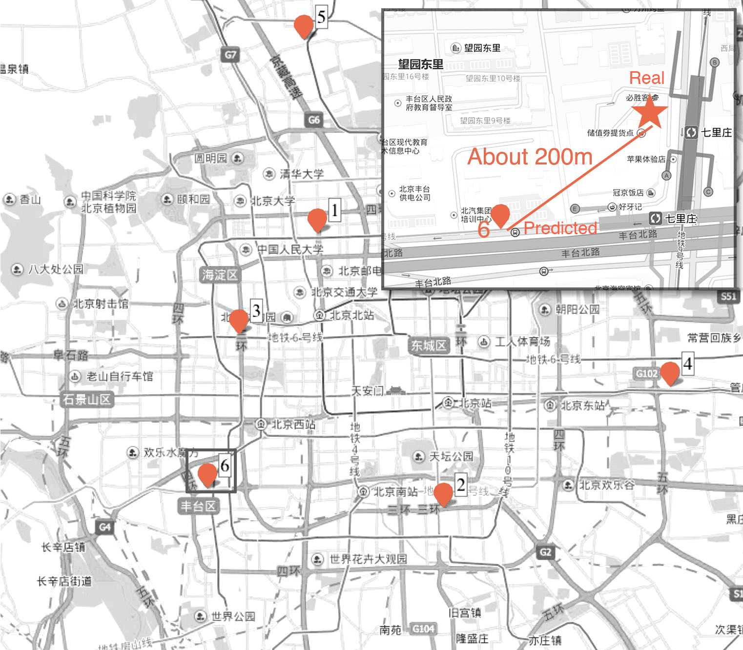
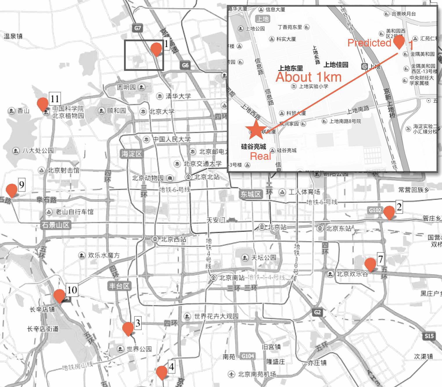
Now we study two real cases which can somehow reflect the effectiveness of our framework(both the obtaining demands part and the learning part). The two cases are “Starbucks” opened at January, 2016 and chain hotpot restaurant “HaiDiLao” opened at September, 2015. We obtain the location with demands using the map query data from April, 2015 to June, 2015 which is far early from the existence of two new stores. The locations with demands of “Starbucks” and “HaiDiLao” are shown in Figure 11(a) and Figure 11(b), respectively. Note that we exclude the existing store opened at that time. We train the Random Forests model using the two brands of existing chain stores. The ranking of the locations with demands of “HaiDiLao” is [‘4’, ‘1’, ‘9’, ‘2’, ‘6’, ‘12’, ‘5’, ‘11’, ‘8’, ‘10’, ‘7’, ‘3’], and the distance between location ‘1’ which is in the top-3 of the ranking list and the new opened store is about 1km. For “Starbucks”, the predicted ranking list is [‘2’, ‘6’, ‘5’, ‘4’, ‘1’, ‘3’] . Location ‘6’ is only 200m away from the real location.
6 Related work
The store placement problem has be studied by researchers from various fields. Researchers have concentrated on various techniques including spatial interaction models, Multiple regression Discriminant analysis and so on [11] . Spatial interaction models are based on the assumptions that the intensity of interaction between two locations decreases with their distance and that the usability of a location increases with the intensity of utilization and the proximity of complementarily arranged locations [1, 2, 25, 15]. Specifically, work in [15] employs spatial interaction theory, customer density estimates and minimax decision criterion to address site selection issues. Authors of [2, 25] utilize theoretic models of optimal location by maximizing the number of residents it can attracts in Euclidean space or road network. By saying a location attracts a resident, we mean that the location is closest to the place the resident live among all the existing stores. However, in reality, people are moving and the location can attracts not only residents near it. Multiple regression Discriminant analysis [21] is a location analyst that has been employed to produce a series of sales forecasts for both new and existing stores, which is tested and calibrated across a number of different scenarios and is often used as a benchmarking tool for future development. Jensen [13] proposed a spatial network based formulation of the problem, where nodes are differrient types of retail stores and weighted signed links are defined to model the attraction and repulsion of entities in the network.
Location based services have been widely used in the analysis of trade and location placement [14, 20]. Karamshuk et al. [14] find optimal retail store location from a list of locations by using supervised learning with features mined from Foursquare check-in data. Researchers in [17] focus on locating the ambulance stations by using the real traffic information so as to minimize the average travel-time to reach the emergency requests. The authors of [20] illustrate how User Generated Mobile Location Data like Foursquare check-ins can be used in trade area analysis. [8] exploits regression modeling, pairwise ranking objective and sparsity regularization to solve the real estate ranking problem with online user reviews and offline moving behaviors. Also authors in [9] propose a method for estate appraisal by leveraging the mutual enforcement of ranking and clustering power.
Previous work of finding optimal location do not consider the activity demand of users. [24] predicts users’ activity via integrating data of map query and mobility trace, which concludes the fact that map query data can be seen as demands and signals of users doing the activity. Rogers [22] proposed some key elements of a retail location study including competition, transportation, trade area definition and so on. Inspired by the above work, we combine users’ geodemand with supervised learning [14] using geographic and consumptive information (some key elements) mined from multiple real data sources.
7 Conclusion
In this paper, we propose a novel framework D3SP for the optimal store placement problem. Our framework combines the spatial distribution of user demands with the popularity and economic attributes of each location. Also the integration of multiple data sources enables us to extract rich features from existing stores. The evaluation results demonstrate the effectiveness of our proposed method for optimal store placement in both experiments and real life business scenarios.
References
- [1] A. Athiyaman. Location decision making: the case of retail service development in a closed population. In Academy of Marketing Studies, volume 15, page 13, 2010.
- [2] O. Berman and D. Krass. The generalized maximal covering location problem. Computers & Operations Research, 29(6):563–581, 2002.
- [3] L. Breiman. Random forests. Machine learning, 45(1):5–32, 2001.
- [4] C. J. Burges. From ranknet to lambdarank to lambdamart: An overview. Learning, 11:23–581, 2010.
- [5] Z. Chen, Y. Liu, R. C.-W. Wong, J. Xiong, G. Mai, and C. Long. Efficient algorithms for optimal location queries in road networks. In Proceedings of the 2014 ACM SIGMOD international conference on Management of data, pages 123–134. ACM, 2014.
- [6] D. Comaniciu and P. Meer. Mean shift: A robust approach toward feature space analysis. Pattern Analysis and Machine Intelligence, IEEE Transactions on, 24(5):603–619, 2002.
- [7] J. H. Friedman. Greedy function approximation: a gradient boosting machine. Annals of statistics, pages 1189–1232, 2001.
- [8] Y. Fu, Y. Ge, Y. Zheng, Z. Yao, Y. Liu, H. Xiong, and N. J. Yuan. Sparse real estate ranking with online user reviews and offline moving behaviors. In Data Mining (ICDM), 2014 IEEE International Conference on, pages 120–129. IEEE, 2014.
- [9] Y. Fu, H. Xiong, Y. Ge, Z. Yao, Y. Zheng, and Z.-H. Zhou. Exploiting geographic dependencies for real estate appraisal: A mutual perspective of ranking and clustering. In Proceedings of the 20th ACM SIGKDD International Conference on Knowledge Discovery and Data Mining, KDD ’14, pages 1047–1056, New York, NY, USA, 2014. ACM.
- [10] M. A. Hearst, S. T. Dumais, E. Osman, J. Platt, and B. Scholkopf. Support vector machines. Intelligent Systems and their Applications, IEEE, 13(4):18–28, 1998.
- [11] T. Hernandez and D. Bennison. The art and science of retail location decisions. International Journal of Retail & Distribution Management, 28(8):357–367, 2000.
- [12] K. Järvelin and J. Kekäläinen. Cumulated gain-based evaluation of ir techniques. ACM Transactions on Information Systems (TOIS), 20(4):422–446, 2002.
- [13] P. Jensen. Network-based predictions of retail store commercial categories and optimal locations. Physical Review E, 74(3):035101, 2006.
- [14] D. Karamshuk, A. Noulas, S. Scellato, V. Nicosia, and C. Mascolo. Geo-spotting: Mining online location-based services for optimal retail store placement. In Proceedings of the 19th ACM SIGKDD international conference on Knowledge discovery and data mining, pages 793–801. ACM, 2013.
- [15] A. Kubis and M. Hartmann. Analysis of location of large-area shopping centres. a probabilistic gravity model for the halle–leipzig area. Jahrbuch für Regionalwissenschaft, 27(1):43–57, 2007.
- [16] J. Li and A. Deshpande. Consensus answers for queries over probabilistic databases. In Proceedings of the twenty-eighth ACM SIGMOD-SIGACT-SIGART symposium on Principles of database systems, pages 259–268. ACM, 2009.
- [17] Y. Li, Y. Zheng, S. Ji, W. Wang, Z. Gong, et al. Location selection for ambulance stations: a data-driven approach. In Proceedings of the 23rd SIGSPATIAL International Conference on Advances in Geographic Information Systems, page 85. ACM, 2015.
- [18] K. P. Murphy. Machine learning: a probabilistic perspective. MIT press, 2012.
- [19] F. Pedregosa, G. Varoquaux, A. Gramfort, V. Michel, B. Thirion, O. Grisel, M. Blondel, P. Prettenhofer, R. Weiss, V. Dubourg, J. Vanderplas, A. Passos, D. Cournapeau, M. Brucher, M. Perrot, and E. Duchesnay. Scikit-learn: Machine learning in Python. Journal of Machine Learning Research, 12:2825–2830, 2011.
- [20] Y. Qu and J. Zhang. Trade area analysis using user generated mobile location data. In Proceedings of the 22nd international conference on World Wide Web, pages 1053–1064. International World Wide Web Conferences Steering Committee, 2013.
- [21] D. Rogers. Site for store buys. New Perspectives, 5:14–17, 1997.
- [22] D. S. Rogers. Retail location analysis in practice. Research Review, 14(2):73–78, 2007.
- [23] S. Wood and J. Reynolds. Leveraging locational insights within retail store development? assessing the use of location planners? knowledge in retail marketing. Geoforum, 43(6):1076–1087, 2012.
- [24] Z. Wu, H. Wu, and T. Zhang. Predict user in-world activity via integration of map query and mobility trace. In UrbComp’15, 1991.
- [25] X. Xiao, B. Yao, and F. Li. Optimal location queries in road network databases. In Data Engineering (ICDE), 2011 IEEE 27th International Conference on, pages 804–815. IEEE, 2011.