Consistency of the growth rate in different environments with
the 6dF Galaxy Survey:
measurement of the void-galaxy &
galaxy-galaxy correlation functions
Abstract
We present a new test of gravitational physics by comparing the growth rate of cosmic structure measured around voids with that measured around galaxies in the same large-scale structure dataset, the low-redshift 6-degree Field Galaxy Survey. By fitting a Redshift Space Distortion model to the 2D galaxy-galaxy and void-galaxy correlation functions, we recover growth rate values and , respectively. The environmental-dependence of cosmological statistics can potentially discriminate between modified-gravity scenarios which modulate the growth rate as a function of scale or environment and test the underlying assumptions of homogeneity and isotropy.
I Introduction
Galaxy peculiar velocities are a powerful probe of gravitational physics. They are sourced by virialized motion within halos and the overall bulk-flow motions due to gravitational interactions, leading to the mass assembly of halos. Although direct measurement of galaxy peculiar velocities is challenging, their correlated effect is imprinted in the clustering of matter through Redshift Space Distortion (RSD), allowing us to determine the linear growth rate of structure. This quantity describes the growth of matter perturbations through cosmic evolution, containing critical information on cosmic expansion and gravitational physics.
For standard General Relativity (GR), in homogeneous and isotropic cosmologies, the growth rate in linear perturbation theory does not depend on the comoving spatial scale Peebles and can be approximated by where is the matter density parameter at redshift , and is a constant. For a CDM Universe , independently of scale and environment. This would not be the case for different cosmological scenarios. For instance, inhomogeneous models of dark energy can lead to patches of clustered dark energy (e.g. Vernizzi2015 , DuttaMaor2007 ) which will have different expansion histories, or certain models of modified gravity such as Hu_Sawicki_2007 rely on the Chameleon effect (Khoury_Weltman_2004, ) that suppresses the gravitational force in under-dense environments. These theories would naturally lead to an environmentally-dependent growth rate and possibly a breakdown of the cosmological isotropy of our universe. As pointed out in Caietal2016 , the scale on which the environment is defined is important. For very large under-dense regions, the effective cosmological parameters are expected to be different to the global-averaged parameters, but the quantification of this critical scale can also serve as an interesting test for departures from Einstein gravity.
A simple test of this physics is to compare the growth rate around cosmic voids to that inferred from galaxy clustering. In fact, non-linear dynamics are expected to be reduced in cosmic voids compared to galaxy clustering in overdense regions Hamaus2016 . Hence cosmic voids can potentially provide powerful tests of cosmology, for instance using the integrated Sachs-Wolfe effect SachsWolfe1967 (e.g. Granett2008 ), the Alcock-Paczynski test Alcock-Paczynski1979 (e.g. LavauxWandelt2012 ) or void abundance and density profile (e.g. ANP ; IA_voidfinder ; ABPW ; Clampittetal2013 ; Zivicketal2015 ).
In this work we test the consistency of the growth rate with environment using RSD measurements around voids and galaxies in the 6-degree Field Galaxy Survey (6dFGS) Jones2004 ; Jones2006 , a low-redshift large-scale structure dataset. There are several advantages to performing these tests near . First, cosmic expansion is dominated by dark energy, hence a measurement of the growth rate around cosmic voids is a particularly interesting test of dark energy clustering. Second, the impact of the Alcock-Paczynski effect at is minimal, such that our measurements have little sensitivity to the assumed cosmology. Third, low-redshift surveys such as the 6dFGS have a much higher galaxy number density than high-redshift surveys, enabling a higher-resolution measurement of the density field. This is particularly important for identifying voids in an unbiased fashion. Finally, the 6dFGS also contains a set of direct galaxy peculiar velocity measurements derived using fundamental-plane distances Springob2014 . Although we don’t use these measurements in the present work, they offer interesting opportunities for future investigation.
The measurement of the growth rate using RSD in galaxy clustering has been previously investigated for many datasets including the 6dFGS Beutler6dF , the 2dF Galaxy Redshift Survey (2dFGRS) (Peacock2001, ; Hawkins2003, ; Cole2005, ), the Sloan Digital Sky Survey (SDSS) (Tegmark2006, ), the WiggleZ Dark Energy Survey Blake2011 , the Baryon Oscillation Spectroscopic Survey (BOSS) (Reid2012, ; Reid2014, ; Beutler2014, ) and the VIMOS Public Extragalactic Redshift Survey (VIPERS) delaTorre2013 . These measurements have shown a general consistency with the CDM cosmological model, up to a precision, albeit in some cases showing tension with the predictions of the latest Cosmic Microwave Background measurements Planck_cosmo . However, the measurement of the growth using RSD in void-galaxy clustering has not been widely investigated, although Hamaus2016 and Adam_viper recently reported measurements using the BOSS-CMASS sample and VIPERS, respectively. However, none of these studies has explored the consistency of the growth rate in different environments using the same galaxy survey.
This paper is organized as follows: in section II we describe the model we use to fit the measurement of the galaxy-galaxy and void-galaxy correlation functions. In section III we test these models using mock catalogues. In section IV we apply our framework to the 6dFGS data and deduce constraints on the growth rate in different environments, and we conclude in section V.
II Models for the 2D correlation functions
The peculiar velocities of galaxies, , due to the local gravitational potential, result on small scales in random motions of galaxies within a group. By measuring galaxy positions in redshift space, we can observe the well-known ‘Finger-of-God’ (FoG) effect. On large scales, the bulk flow (coherent infall/outflow in overdense/underdense regions) is responsible for an overall coherent distortion known as the ‘Kaiser effect’ Kaiser1987 .
The mapping of the position of a galaxy from real space to its position in redshift space is given by:
| (1) |
where is the unitary vector along the line of sight, and is the Hubble parameter at redshift . On large scales, where the matter overdensity grows coherently Kaiser1987 ; Hamilton1992 , linear perturbation theory implies that where is the matter density contrast and the linear growth rate of perturbations is defined as:
| (2) |
We need to relate the observed galaxy overdensity, , to the matter density contrast, which we accomplish using a linear bias , which is independent of scale in the linear regime.
In what follows we use the notation for the component of galaxy-galaxy or void-galaxy separation perpendicular to the line of sight, and for the component parallel to the line of sight. For both the galaxy-galaxy and the void-galaxy correlation functions, the random small-scale component of the peculiar velocity can be described by convolving the correlation function with a pairwise velocity distribution Peebles . The latter is often modelled as a Gaussian or Lorentzian distribution; we consider both choices in our analysis.
The galaxy-galaxy correlation function
The redshift-space 2D correlation function due to the coherent bulk flow of peculiar velocity can be described by Kaiser1987 ; Hamilton1992 :
| (3) |
where are Legendre polynomials and is the angle between the separation vector and line of sight. In the linear regime Kaiser1987 ,
where , the real-space matter correlation function is , and
Including our model for small-scale random motions, the total 2D correlation function in redshift space is given by Peebles
| (4) |
where is the probability distribution of the random pairwise motions. In what follows we model the matter clustering using the non-linear power spectrum from CAMB (halofit) Lewis_camb and Fourier transform it to obtain the non-linear matter correlation function in Eq.4. We adopt a fiducial cosmology matching that of Mocks A described below: a flat WMAP 5-year cosmology wmap (, , , , ).
The void-galaxy correlation function
The previous effects of the peculiar velocity also apply to the void-galaxy correlation function and we have Peebles :
| (5) |
where is the angle-averaged void-galaxy correlation function in real space and .
We calibrate the model using the real-space void-matter cross-correlation measured from N-body simulations (see section III) as our CDM template, such that including the linear bias factor
| (6) |
For coherent outflow motion, at linear order, the peculiar velocity can be expressed as Peebles :
| (7) |
where is the average integrated density contrast around voids. For spherical voids we have
| (8) |
The pairwise velocity distribution
In this work we will consider two models and to describe the pairwise velocity distribution in Eq.4,5: model G will use a Gaussian distribution given by
| (9) |
while model L will use a Lorentzian distribution (in Fourier space) which corresponds to convolution by an exponential distribution in configuration space:
| (10) |
where is the standard deviation of the peculiar velocity. Our model hence neglects the scale dependence of (Hamaus_simuanalysis, ; Koppetal2016, ; IA_voidfinder, ).
A Gaussian distribution of peculiar velocities is often assumed for the random motions which result from halo relaxation. However, numerical studies (e.g. Takashi ) have shown that a Lorentzian distribution can provide a better empirical description of the distribution of peculiar velocities which might result from a superposition of different-mass haloes.
Summary of the variables
Our model hence consists of 3 parameters for both the galaxy-galaxy and void-galaxy correlation functions: the linear bias which enters into Eq.3,6, the standard deviation of the peculiar velocity that enters into Eq.9,10, and the linear growth rate that is part of Eq.3,7. We note that, in the linear-theory approximation, the fitted values of and are degenerate with the assumed normalization of the matter power spectrum, . We reflect this degeneracy by presenting our results in terms of the normalized variables and .
Remarks on the models
The RSD models we use in our study, whilst commonly-adopted in the literature, greatly simplify the non-linear physics which will be present on these scales. For example, galaxy bias generally exhibits non-linear, non-local, scale-dependent and stochastic properties Desjacques2016 and the galaxy pairwise velocity dispersion may be scale-dependent or non-Gaussian Hamaus_simuanalysis ; Koppetal2016 ; IA_voidfinder . However, in the following section we will use mock catalogues to demonstrate that, at the level of statistical precision of the 6dFGS dataset, these simple models are sufficient to extract unbiased estimates of the growth rate from both the galaxy-galaxy and void-galaxy correlations. Many studies have confirmed this conclusion through comparison with more sophisticated models (e.g. Beutler6dF , in the context of 6dFGS). More accurate modelling of RSD is a significant challenge for upcoming galaxy surveys with much greater statistical precision such as Euclid EUCLIDsurvey .
III Tests on mocks
In order to test our analysis pipeline and the limitations of our models, we measured the growth rate in two sets of mock catalogues. Mocks A are flat-sky mocks with no survey selection function applied, for which we possess the full set of dark matter and halo information. We used these mocks to model the extraction of galaxy voids from a volume-limited observational sample and the fitting of the void-galaxy correlation function. Mocks B are curved-sky mocks which incorporate the full 6dFGS selection function via detailed halo-occupation modelling. Although we do not have the dark matter information to allow tests of the void sample, we used these mocks to test the fitting of the galaxy-galaxy correlation function to the flux-limited observational sample. We summarize the creation of these two sets of mocks below.
Mocks A: volume-limited samples
To generate Mocks A, we used a sample of dark matter particles and halos from the DEUSS simulations DEUSS . These simulations were run for several scientific purposes, as described in Alimi ; Rasera ; Achitouv and are freely available. The simulations were carried out using the RAMSES code RAMSES for a CDM model calibrated to the WMAP 5-year cosmological parameters wmap . We used the output of a simulation generated in a Mpc3 box using particles.
In section IV we will extract galaxy voids from a volume-limited sample of 6dFGS galaxies. We built a series of 20 dark matter () catalogues approximately matching the number density and volume of this sub-sample, by randomly-selecting DM particles a box of side-length Mpc. We also built 20 biased galaxy mocks by sub-sampling halos identified with the Friend-of-Friends (FoF) algorithm with linking length , selecting the most massive haloes in order to approximately mimic the 6dFGS selection. Finally, in order to simulate the RSD we used the flat-sky approximation and shifted the positions of the DM particles and halos according to Eq.1, using their peculiar velocities.
We note that, when generating these mocks, it is important to match the DM and halo number density to the galaxy dataset in order to avoid introducing a bias in the identification of voids between the mock and the real dataset. For instance, in Caietalbias , the authors show that the density profile of voids is sensitive to the resolution of the simulation.
Mocks B: selection-function samples
In section IV we will use the magnitude-limited 6dFGS sample to measure RSD from the galaxy-galaxy correlations. We therefore supplemented Mocks A with a second simulation set, Mocks B, which provided a more accurate curved-sky modelling of the survey selection function and redshift-dependence of the galaxy bias.
We built Mocks B from the COLA N-body simulations introduced by Koda2016 , using a modified version of the pipeline created by Beutler2016 to construct BOSS and WiggleZ mocks. In brief, we first fit the central and satellite galaxy halo occupation distribution of the 6dFGS galaxy sample as a function of luminosity Beutler2013 . By calibrating the luminosity-redshift relation, we defined the redshift-evolution of the HOD. Through careful comparison of the projected and 3D clustering of the mock and data sample, we iterated the HOD parameters to produce the closest possible match. We then applied peculiar velocities along the line-of-sight, and sub-sampled the resulting distribution with the 6dFGS angular selection function BeutlerBAO . These mocks will be presented in more detail by Carter2017 .
Void-finding in Mocks A
In our analysis we identified voids with radius Mpc using the void finder developed by IA_voidfinder . This radius is chosen as a compromise between being small enough to obtain sufficient voids for an accurate measurement of the void-galaxy correlation function, but being large enough to select genuinely underdense patches of matter Sutter_smallvoids .
This void finder uses density criteria to identify voids with the characteristic profile illustrated by Fig.1. For each of the candidate void positions, which are picked at random, the algorithm first requires that the overdensity is below a threshold in two central bins, and , where Mpc and Mpc. The third condition ensures a ridge of the void profile by requiring that and the fourth condition controls the amplitude of the ridge by requiring that .
We used 10 times the number of candidate positions as tracers, producing a sample of voids for each Mock A, which is similar to the number density of voids we find by applying the same algorithm to the volume-limited 6dFGS sub-sample. We note that about half these voids have some portion of overlap; this does not affect our analysis because overlap does not change the radial density profile IA_voidfinder , and any covariance between overlapping voids is already encoded in the measurement scatter between mocks.
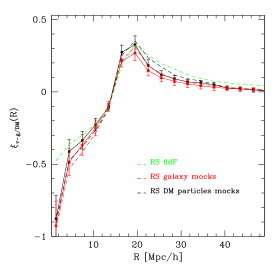
1D matter-void cross-correlation function
We measured the void-tracer cross-correlation functions using the Landy-Szalay estimator:
| (11) |
where is the number of data void-galaxy pairs, the random void-galaxy pairs and the number of galaxy/void data-random pairs, in a bin at separation . The total number of galaxies, voids, galaxy-randoms and voids-randoms are , , and , respectively. In all cases we generated random catalogues having 10 times the number of galaxies than our data samples.
The 1D mock mean void-matter correlation function, , is displayed in Fig.1 as the black data points. We also show the void-halo correlation function (red points), using voids identified in real-space mocks before applying RSD. In addition we compare the same measurements after RSD is applied (dashed lines), including the 6dFGS measurement. For clarity we do not show the errors in the redshift-space measurements, which are similar to the real-space case. We see that RSD accentuates the features of the void profile: it makes the inner density profile steeper and the ridge higher.
 |
 |
 |
 |
Model fits to the mock 2D correlation functions
We computed the 2D void-halo correlation function for Mocks A, and the halo-halo correlation functions for both Mocks A & B, using the LS estimator of Eq.11. Indeed, it is interesting to also measure the galaxy-galaxy correlation in mocks A in order to: (i) test if the inferred linear bias is the same as the one inferred from the galaxy-void measurement. (ii) Confirm that the inferred value of the growth rate is the same as the one inferred from the galaxy-void clustering. In fact, there should be a limit of the void size where non-linear effects should impact the value of the growth rate inside large voids. Hence we checked that this effect does not occur for our selected voids by testing the consistency of the growth rate within the same mocks A. When measuring the correlation function for Mocks B, which include the varying survey selection function, we used minimum variance weights FeldmanKP ; Beutler6dF
| (12) |
where (following Beutler6dF ) Mpc3 and is the galaxy number density at the location of the object. In Eq.11, the ratio of random objects to data objects then becomes
| (13) |
We computed the 2D correlation functions of 20 mocks in bins of width Mpc in the range Mpc, and used these measurements to construct the standard deviation in each bin, .
For our first analysis we fitted the model to the mock mean 2D correlation function, with an error in each bin given by . This allows us to perform precise systematics tests of Eq.4,5, using a mock dataset with a statistical error far smaller than the real 6dFGS dataset.
At small scales the galaxy-galaxy correlation function is dominated by the FoG effect, which can not be described by the linear theory and pairwise velocity dispersion models of Eq.4. Therefore, small bins are often excluded when computing the (Eq.14). For these reasons we apply a cut Mpc when fitting the galaxy-galaxy correlation function, while we keep all the separation bins for the void-galaxy correlation function. We consider below the sensitivity of our results to these choices.
We performed our fit using a Metropolis-Hastings Markov Chain Monte Carlo (MCMC) analysis for the parameters , analyzing our Monte Carlo chains using the module GetDist developed by A. Lewis Lewis . We used priors , and km s-1, although our results are not sensitive to these choices. We computed the likelihood of each model assuming
| (14) |
We cannot numerically determine the large covariance matrix between different bins sufficiently accurately to allow it to be inverted when determining the statistic, so in Eq.14 we assumed no correlation between bins. Our MCMC fit will therefore not produce robust parameter errors, and we instead used the dispersion of the best-fitting parameter values between individual mocks, , as a more accurate estimate of the resulting errors. This scatter, which is typically double the parameter error obtained by the MCMC, naturally includes the effect of data correlations. When fitting to the mock mean, we report a scaled parameter error .
We report the best-fitting parameter values and errors of our fits to the mock mean galaxy-galaxy and void-galaxy correlation functions, and minimum values, in Tab.1. We find that both the Gaussian and the Lorentzian models lead to similar constraints on the growth rate, and that the best-fitting growth rates are consistent with the fiducial cosmology of the mocks (), validating our models. The fits to Mocks A show that the fiducial growth rate is recovered around both voids and galaxies for a consistent tracer population, and that our choice of void size produces no unwanted systematic effect due to non-linearity or inhomogeneity. The best-fitting values are high for both statistics, although we note that these values neglect the off-diagonal elements of the covariance matrix, and that the mock mean provides a far more precise diagnostic of systematics than the real survey data.
The galaxy-galaxy RSD provides weaker constraints on than the void-galaxy correlation function, due to our exclusion of small scales from the fit in this case. The error in is sensitive to this cut, as we will see in Fig.4. Tab.1 also lists best-fitting values for the galaxy bias factor. We note that the galaxy bias factor for Mocks B is significantly higher than for Mocks A, because of the selection of more massive halos required to match the 6dFGS sample at higher redshifts, and the upweighting of those halos by the FKP weights. The comparison of the results of the void-galaxy and galaxy-galaxy correlation function fits for Mocks A allows us to verify that the measured tracer bias is consistent in the two cases, implying that there is not a environmental dependence of this parameter.
| Mocks | ||||||||
|---|---|---|---|---|---|---|---|---|
| A | ||||||||
| A | ||||||||
| A | ||||||||
| A | ||||||||
| B | 1.01 | |||||||
| B | 1.00 |
| Mocks | ||||
|---|---|---|---|---|
| A | ||||
| A | ||||
| A | ||||
| A | ||||
| B | ||||
| B |
In Tab.2 we report summary statistics of the fits of our model to the individual mock catalogues, listing the mean values of the best-fitting parameters (, , ) and their dispersion across the mock catalogues (, , ). The mean values are consistent with the best fit to the mock mean, indicating that our approach is unbiased.
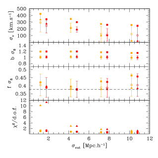
We checked the dependence of the best-fitting parameter values on the range of scales included in our analysis. In the upper panel of Fig.4, we show the variation of the best-fitting values with the cutting scale , for the fits to the galaxy-galaxy correlation function of Mocks B. The triangles (red for model and orange for model ) show the result from fitting to the mock mean, while the unfilled circles correspond to the mean parameter fit to the individual mocks. The minimum reduced is shown in the bottom panel. Deviations are seen when including the first bin, which we expect to be most strongly affected, although our results do not show a strong dependence on and we adopt a baseline Mpc for our analyses.
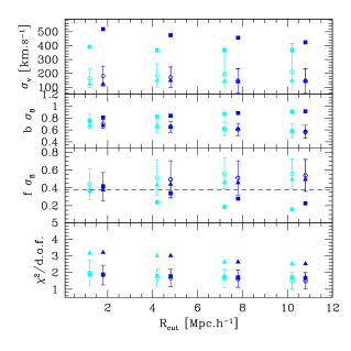
A similar analysis of the void-galaxy correlation function of Mocks A is shown in the lower panel of Fig.4 where, given the absence of non-linear pairwise velocities, we now consider a cut as a function of the total separation, . This is motivated by the possibility that linear theory may break down at the centre of the voids where Caietal2016 . We plot the best-fitting parameters as a function of as well as the reduced for model (blue lines) and model (cyan lines). The fits to the mock mean are shown by the triangles, while the unfilled circles correspond to the mean parameter fit to the individual mocks. In this case, we find a low sensitivity of the results to the value of . The best-fitting parameters are consistent with our fiducial cosmology when we use all scales in Eq.14.
IV Application to 6dFGS
 |
 |
 |
 |
Galaxy and void samples
The 6dF Galaxy Survey was undertaken with the multi-fibre instrument on the UK Schmidt Telescope between 2001 and 2006. The median redshift of the survey is and it covers nearly the entire southern sky. A full description of the survey can be find in Jones2004 ; Jones2006 including comparisons between 6dFGS, 2dFGRS and SDSS. In this analysis we utilized the same -band selected 6dFGS sub-sample, consisting of galaxies, as constructed for the analysis of the baryon acoustic peak by BeutlerBAO . We also used random catalogues following the same angular and redshift selection as the data sample, generated by BeutlerBAO .
We constructed different 6dFGS sub-samples for analyzing the galaxy-galaxy and void-galaxy correlation functions. For the measurement of the void-galaxy correlation function, we first constructed a volume-limited catalogue corresponding to an approximately constant number density. This step is crucial in order to apply our measurement of the 1D real-space void-matter correlation function in Eq.6, and to avoid any evolution in the void properties with redshift. We built the volume-limited catalogue by determining the absolute magnitude of each galaxy using
| (15) |
where is the apparent -band magnitude, is the luminosity distance in Mpc and is the -correction 0210394v1 ; Mannucci2001 . For this analysis we set the maximum redshift of the sample to , in order to obtain a sample with a sufficiently high number density. The faint magnitude limit of the survey is , and we selected all galaxies brighter than in the redshift range , where is computed from Eq.15 with . We identified voids in the catalogue using the algorithm described in Sec.III, leading to the identification of voids.
Measurement of the correlation function
We transformed the angular co-ordinates and redshifts of the galaxies to co-moving Cartesian coordinates assuming the same fiducial cosmology as our mock catalogue , although we note that the Alcock-Paczynski effect is negligible at low redshift. The separation of two galaxies along the line of sight and across the line of sight is measured in the same manner as Mocks B using
| (16) |
where is the separation of the galaxies in redshift space and is the mean distance to the galaxy pair.
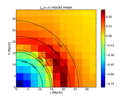
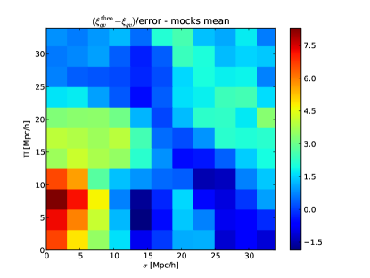
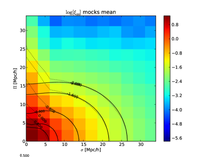
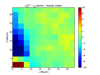
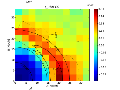
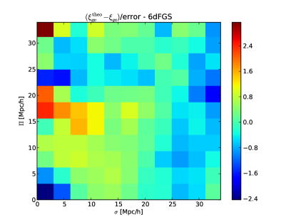
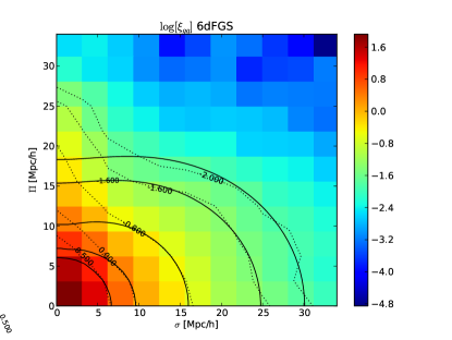
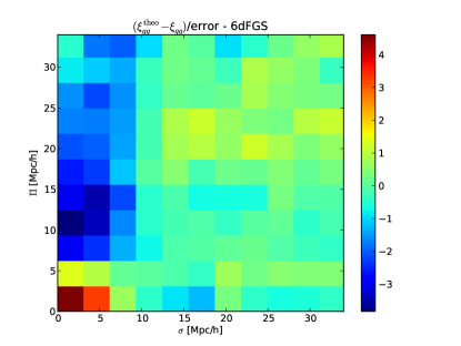
Fig.3 displays the measured 2D galaxy-galaxy correlation function (lower left) and void-galaxy correlation function (lower right) for the 6dFGS dataset. For the galaxy-galaxy correlation function, we can see the elongation at small scales along the line of sight (FoG), due to the random motion of galaxies within halos. On larger scales, we observe the Kaiser effect due to coherent bulk flows. For the void-galaxy correlation function, we can detect an apparent asymmetry within the void ( Mpc): the ‘emptiness’ is larger along the line of sight due to the cosmic expansion, and the ridge of the void ( Mpc) tends to be erased due to the velocity dispersion. The Kaiser effect can also be observed: the signal is enhanced across the line of sight, especially on the ridge.
We obtained the error in the 6dFGS void-galaxy and galaxy-galaxy correlation functions using the dispersion in the measurements from Mocks A and B, respectively. We scaled the standard deviation of the void-galaxy mock measurements to allow for the slightly different volumes of Mock A and the real dataset:
| (17) |
where Mpc3 and the scaling factor is . The parameter errors are also scaled by this correction factor. No volume-scaling is needed for the galaxy-galaxy correlation functions, since Mocks B sample the exact survey selection function.
Growth rate measurement in different environments
We fitted our RSD model to the 6dFGS data using the MCMC pipeline described in Section III. As previously discussed, we obtain robust parameter errors using the dispersion of the fits to the mock catalogues.
We report the best-fitting parameter values and their errors in Tab.3. Our measurement of the growth rate for the average of models L and G is for the galaxy-galaxy RSD and for the void-galaxy RSD. We observe larger uncertainties in the growth rate measured using the void-galaxy correlation function, although the two measurements are consistent within the statistical errors. The minimum values, also listed in Tab.3, are lower than those found for the more accurate mock mean dataset, but we note that they are still impacted by the assumption of a diagonal covariance matrix. The right-hand panels of Figure 3 show the residuals between the data and best-fitting models. Our measurement is in very good agreement with the previous 6dFGS galaxy-galaxy RSD analysis Beutler6dF , which obtained .
The difference in the best-fitting bias parameters for and is due to the different galaxy samples used: for the galaxy-galaxy analysis we adopt a flux-limited sample across a wider redshift range, and up-weight more luminous, highly-biased galaxies. The best-fitting bias values are comparable with those found in the corresponding mock catalogue analyses in each case, although some differences remain.
These results are obtained with a cut Mpc for the galaxy-galaxy correlation function, and using all bins for the void-galaxy correlation function. This is motivated by the mock-catalogue analysis and the lack of sensitivity of our best-fitting parameters to these choices, which is illustrated by Fig.4. For Mpc, the goodness-of-fit and best-fitting parameters do not significantly change for the galaxy-galaxy correlation function (left panel), independently of the model (see the red/orange solid lines). The best-fitting of the void-galaxy correlation function (right panel) remains unchanged at all scales, independently of the model (see the blue/light blue solid lines).
Overall, the growth rate measurements are consistent between the void-galaxy and galaxy-galaxy RSD. One might think about combining these measurements to improve the uncertainties. However we do not expect a significant improvement since the growth uncertainties from the void-galaxy RSD are double those of the galaxy-galaxy RSD, and the measurements are correlated. Hence, the novelty of our result relies on the comparison of the growth between different environments.
V Conclusion
In this work we provide the first direct comparison of the cosmic growth rate measured in two different environments of the same galaxy survey, by fitting to Redshift Space Distortion in the galaxy-galaxy and void-galaxy correlation functions of the 6-degree Field Galaxy Survey. As a low-redshift survey, our 6dFGS measurements are particularly relevant for probing the late-time domination of dark energy, and are insensitive to the Alcock-Pacynski effect. We find voids using a new void-finder which identifies under-densities matching supplied density profile criteria IA_voidfinder . We also note that our measurement of the growth using RSD around voids is the first performed at low redshift and in the southern hemisphere.
We determine similar growth rate measurements around galaxies () and Mpc underdensities (), finding no evidence of an environmental dependence of gravitational physics. We validate our models, and estimate the errors in our measurements, using mock galaxy catalogues. Extracting the complementary cosmological information present in different environments (AchitouvBlake2015, ; Kitaura2015, ) will be a powerful test of physics for both current galaxy redshift surveys and future projects such as Euclid EUCLIDsurvey .
Our analysis could be extended in several ways: direct measurements of peculiar velocities using standard-candle indicators could further constrain their radial profile around voids; combining our results with analyses of other data sets such as SDSS SDSSsurvey and GAMA Gamasurvey can probe these effects as a function of redshift; and a comparison of our measurements with the predictions of non-standard cosmological models, in particular modified gravity and interacting dark energy models, would place new constraints on those frameworks.
Acknowledgments
We are very grateful to Yann Rasera for facilitating the access to the DEUS N-body simulations.
The 6dF Galaxy Survey was made possible by contributions from many individuals towards the instrument, the survey and its science. We particularly thank Matthew Colless, Heath Jones, Will Saunders, Fred Watson, Quentin Parker, Mike Read, Lachlan Campbell, Chris Springob, Christina Magoulas, John Lucey, Jeremy Mould, and Tom Jarrett, as well as the dedicated staff of the Australian Astronomical Observatory and other members of the 6dFGS team over the years.
Part of this research was conducted by the Australian Research Council Centre of Excellence for All-sky Astrophysics (CAASTRO), through project number CE110001020. We also acknowledge support from the DIM ACAV of the Region Ile-de-France.
References
- (1) Peebles, P. J. E., Principles of Physical Cosmology by P.J.E. Peebles. Princeton University Press, 1993. ISBN: 978-0-691-01933-8
- (2) Gleyzes, Jerome; Langlois, David; Mancarella, Michele; Vernizzi, Filippo, Journal of Cosmology and Astroparticle Physics, Issue 02, article id. 056 (2016).
- (3) Dutta, Sourish; Maor, Irit, Physical Review D, vol. 75, Issue 6, id. 063507 (2007)
- (4) Hu, Wayne; Sawicki, Ignacy, Physical Review D, vol. 76, Issue 6, id. 064004
- (5) Khoury, Justin; Weltman, Amanda, Physical Review D, vol. 69, Issue 4, id. 044026
- (6) Cai, Yan-Chuan; Taylor, Andy; Peacock, John A.; Padilla, Nelson, eprint arXiv:1603.05184
- (7) Hamaus, Nico; Pisani, Alice; Sutter, Paul M.; Lavaux, Guilhem; Escoffier, Stéphanie; Wandelt, Benjamin D.; Weller, Jochen, eprint arXiv:1602.01784
- (8) Sachs, R. K.; Wolfe, A. M., Astrophysical Journal, vol. 147, p.73 (1967)
- (9) Granett, Benjamin R.; Neyrinck, Mark C.; Szapudi, Istvan, The Astrophysical Journal Letters, Volume 683, Issue 2, article id. L99, pp. (2008)
- (10) Charles Alcock & Bohdan Paczynski, Nature 281, 358 - 359 (04 October 1979)
- (11) Lavaux, Guilhem; Wandelt, Benjamin D., The Astrophysical Journal, Volume 754, Issue 2, article id. 109, 15 pp. (2012)
- (12) Achitouv, Ixandra; Neyrinck, Mark; Paranjape, Aseem, Monthly Notices of the Royal Astronomical Society, Volume 451, Issue 4, p.3964-3974 (2015)
- (13) Achitouv, Ixandra; Baldi, Marco; Puchwein, Ewald; Weller, Jochen, Phys. Rev. D 93, 103522 (2016), arXiv:1511.01494
- (14) Clampitt J., Cai Y.-C., Li B., 2013, MNRAS, 431, 749
- (15) Zivick, Paul; Sutter, P. M.; Wandelt, Benjamin D.; Li, Baojiu; Lam, Tsz Yan, Monthly Notices of the Royal Astronomical Society, Volume 451, Issue 4, p.4215-4222
- (16) Jones D. H. et al., MNRAS 355 (2004) 747
- (17) Jones D. H., Peterson B. A., Colless M. and Saunders W., MNRAS 369 (2006)
- (18) Springob, C et al. Monthly Notices of the Royal Astronomical Society, Volume 445, Issue 3, p.2677-2697 (2014).
- (19) Beutler, Florian; Blake, Chris; Colless, Matthew; Jones, D. Heath; Staveley-Smith, Lister; Poole, Gregory B.; Campbell, Lachlan; Parker, Quentin; Saunders, Will; Watson, Fred, Monthly Notices of the Royal Astronomical Society, Volume 423, Issue 4, pp. 3430-3444
- (20) Peacock, John A. et al, Nature, Volume 410, Issue 6825, pp. 169-173 (2001)
- (21) Hawkins, Ed et al, Monthly Notices of the Royal Astronomical Society, Volume 346, Issue 1, pp. 78-96 (2003)
- (22) Cole S. et al., MNRAS 362 (2005) 505
- (23) Tegmark M., Phys. Rev. Lett. 79, 3806 (1997)
- (24) Blake, Chris et al. Monthly Notices of the Royal Astronomical Society, Volume 425, Issue 1, pp. 405-414 (2012)
- (25) Reid, B et al., Monthly Notices of the Royal Astronomical Society, Volume 426, Issue 4, pp. 2719-2737 (2012)
- (26) Beth A. Reid, Hee-Jong Seo, Alexie Leauthaud, Jeremy L. Tinker, Martin White, Mon.Not.Roy.Astron.Soc. 444 (2014) no.1, 476-502
- (27) Beutler, F. et al, Monthly Notices of the Royal Astronomical Society, Volume 443, Issue 2, p.1065-1089 (2014)
- (28) de la Torre, S., et al., A&A, 557, 54 (2013)
- (29) Planck Collaboration, eprint arXiv:1502.01589
- (30) Hawken, A. J. et al., ArXiv:1611.07046
- (31) Kaiser, Nick, Monthly Notices of the Royal Astronomical Society (ISSN 0035-8711), vol. 227, July 1, 1987, p. 1-21
- (32) Hamilton, A. J. S.; Kumar, P.; Lu, Edward; Matthews, Alex, Astrophysical Journal, Part 2 - Letters (ISSN 0004-637X), vol. 374, June 10, 1991, p. L1-L4
- (33) Lewis, Antony; Bridle, Sarah, Astrophysics Source Code Library, record ascl:1106.025
- (34) Komatsu, E. et al. The Astrophysical Journal Supplement, Volume 180, Issue 2, pp. 330-376 (2009)
- (35) Hamaus, Nico; Sutter, P. M.; Lavaux, Guilhem; Wandelt, Benjamin D., Journal of Cosmology and Astroparticle Physics, Issue 11, article id. 036, (2015).
- (36) Michael Kopp, Cora Uhlemann, & Ixandra Achitouv, Physical Review D, Volume 94, Issue 12, id.123522, arXiv:1606.02301
- (37) Hamana, Takashi; Kayo, Issha; Yoshida, Naoki; Suto, Yasushi; Jing, Y. P., Monthly Notice of the Royal Astronomical Society, Volume 343, Issue 4, pp. 1312-1318 (2003)
- (38) Desjacques V., Jeong D., Schmidt F., arXiv:1611.09787 (2016)
- (39) www.euclid-ec.org/
- (40) Courtin, J.; Rasera, Y.; Alimi, J.-M.; Corasaniti, P.-S.; Boucher, V.; Füzfa, A., Monthly Notices of the Royal Astronomical Society, Volume 410, Issue 3, pp. 1911-1931
- (41) Alimi, J.-M.; Füzfa, A.; Boucher, V.; Rasera, Y.; Courtin, J.; Corasaniti, P.-S., Monthly Notices of the Royal Astronomical Society, Volume 401, Issue 2, pp. 775-790.
- (42) Rasera Y. et al., 2014, Monthly Notices of the Royal Astronomical Society, Volume 440, Issue 2, p.1420-1434
- (43) Achitouv, I.; Wagner, C.; Weller, J.; Rasera, Y., Journal of Cosmology and Astroparticle Physics, Issue 10, article id. 077, pp. (2014),
- (44) Teyssier, R.,Astronomy and Astrophysics, v.385, p.337-364 (2002)
- (45) Baldauf, Tobias; Seljak, Uroš; Smith, Robert E.; Hamaus, Nico; Desjacques, Vincent, Physical Review D, vol. 88, Issue 8, id. 083507 (2013)
- (46) Koda J., Blake C., Beutler F., Kazin E., Marin F., MNRAS, 459, 2119 (2016)
- (47) Beutler F., Blake C., Koda J., Marin F., Seo H.-J., Cuesta, A., Schneider D., MNRAS, 455, 3230 (2016)
- (48) Beutler F., et al., MNRAS, 429, 3604 (2013)
- (49) Beutler, Florian; Blake, Chris; Colless, Matthew; Jones, D. Heath; Staveley-Smith, Lister; Campbell, Lachlan; Parker, Quentin; Saunders, Will; Watson, Fred, Monthly Notices of the Royal Astronomical Society, Volume 416, Issue 4, pp. 3017-3032 (2011).
- (50) Carter P. et al., in prep. (2017)
- (51) I. Achitouv, 1609.01284, Phys. Rev. D 94, 103524 (2016), arXiv:1609.01284
- (52) Hamaus, Nico; Wandelt, Benjamin D.; Sutter, P. M.; Lavaux, Guilhem; Warren, Michael S., Physical Review Letters, Volume 112, Issue 4, id.041304 (2014)
- (53) Feldman H. A., Kaiser N. and Peacock J. A., Astrophys. J.426 (1994)
- (54) http://getdist.readthedocs.io/en/latest/
- (55) Hogg, David W.; Baldry, Ivan K.; Blanton, Michael R.; Eisenstein, Daniel J, eprint arXiv:astro-ph/0210394
- (56) Mannucci, F.; Basile, F.; Poggianti, B. M.; Cimatti, A.; Daddi, E.; Pozzetti, L.; Vanzi, L., Monthly Notices of the Royal Astronomical Society, Volume 326, Issue 2, pp. 745-758
- (57) I. Achitouv & C. Blake, Physical Review D, Volume 92, Issue 8, id.083523, arXiv:1507.03584
- (58) Kitaura, F.-S. et al. ArXiv e-prints:1511.4405
- (59) www.sdss.org/
- (60) www.gama-survey.org/