Efficient quadratic penalization through the partial minimization technique

Abstract

Common computational problems, such as parameter estimation in dynamic models and PDE constrained optimization, require data fitting over a set of auxiliary parameters subject to physical constraints over an underlying state. Naive quadratically penalized formulations, commonly used in practice, suffer from inherent ill-conditioning. We show that surprisingly the partial minimization technique regularizes the problem, making it well-conditioned. This viewpoint sheds new light on variable projection techniques, as well as the penalty method for PDE constrained optimization, and motivates robust extensions. In addition, we outline an inexact analysis, showing that the partial minimization subproblem can be solved very loosely in each iteration. We illustrate the theory and algorithms on boundary control, optimal transport, and parameter estimation for robust dynamic inference.

I Introduction

In this work, we consider a structured class of optimization problems having the form

$$\min_{y,u}~{}f(y)+g(u)\qquad\mbox{subject to}\qquad A(u)y=q.$$ (1)

Here, $f\colon\mathbb{R}^{n}\to\mathbb{R}$ is convex and smooth, $q\in\mathbb{R}^{n}$ is a fixed vector, and $A(\cdot)$ is a smoothly varying invertible matrix. For now, we make no assumptions on $g\colon\mathbb{R}^{d}\to\mathbb{R}$, though in practice, it is typically either a smooth or a ‘simple’ nonsmooth function. Optimization problems of this form often appear in PDE constrained optimization [23, 21, 6], Kalman filtering [15, 2, 4], boundary control problems [11, 19], and optimal transport [13, 1]. Typically, $u$ encodes auxiliary variables while $y$ encodes the state of the system; the constraint $A(u)y=q$ corresponds to a discretized PDE describing the physics.

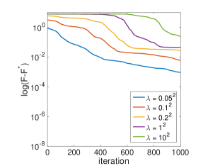
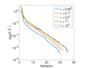
Figure 1: Top panel shows $\log(F_{k}-F^{*})$ of L-BFGS with partial minimization applied to (2) for the boundary control problem in Section III. Each partial minimization solves a least squares problem in $y$. Bottom panel shows $\log(F_{k}-F^{*})$ of L-BFGS without partial minimization applied to (2), for the same values of $\lambda$. Both methods are initialized at random $u$, and $y$ that minimizes $F(\cdot,u)$). Performance of L-BFGS without partial minimization degrades as $\lambda$ increases, while performance of L-BFGS with partial minimization is insensitive to $\lambda$.

Since the discretization $A(u)y=q$ is already inexact, it is appealing to relax it in the formulation. A seemingly naive relaxation approach is based on the quadratic penalty:

$$\min_{y,u}~{}F(y,u):=f(y)+g(u)+\lambda\cdot\|A(u)y-q\|^{2}.$$ (2)

Here $\lambda>0$ is a relaxation parameter for the equality constraints in (1), corresponding to relaxed physics. The classical quadratic penalty method in nonlinear programming proceeds by applying an iterative optimization algorithm to the unconstrained problem (2) until some termination criterion is satisfied, then increasing $\lambda$, and repeating the procedure with the previous iterate used as a warm start. For a detailed discussion, see e.g. [17, Section 17.1]. The authors of [22] observe that this strategy helps to avoid extraneous local minima, in contrast to the original formulation (1). From this consideration alone, the formulation (2) appears to be useful.

Conventional wisdom teaches us that the quadratic penalty technique is rarely appropriate. The difficulty is that one must allow $\lambda$ to tend to infinity in order to force near-feasibility in the original problem (1); the residual error $\|A(u)y-q\|$ at an optimal pair $(u,y)$ for the problem $\eqref{eqn:uncon_form}$ is at best on the order of $\mathcal{O}(1/\lambda)$. Consequently, the maximal eigenvalue of the Hessian of the penalty term scales linearly with $\lambda$ and the problems (2) become computationally difficult. Indeed, the maximal eigenvalue of the Hessian determines the behavior of numerical methods (gradient descent, quasi-Newton) far away from the solution – a regime in which most huge scale problems are solved. Figure 1 is a simple numerical illustration of this inherent difficulty on a boundary control problem; see Section III for more details on the problem formulation. The bottom panel in the figure tracks progress of the objective function in (2) when an L-BFGS method is applied jointly in the variables $(u,y)$. After 1000 iterations of L-BFGS, the objective value significantly increases with increasing $\lambda$, while the actual minimal value of the objective function converges to that of (1), and so hardly changes. In other words, performance of the method scales poorly with $\lambda$, illustrating the ill-conditioning.

In this paper, we show that by using a simple partial minimization step, this complexity blow-up can be avoided entirely. The resulting algorithm is perfectly suited for many large-scale problems, where satisfying the constraint $A(u)y=q$ to high accuracy is not required (or even possible). The strategy is straightforward: we rewrite (2) as

$$\min_{u}~{}\widetilde{\varphi}(u)+g(u),$$ (3)

where the function $\widetilde{\varphi}(u)$ is defined implicitly by

$$\widetilde{\varphi}(u)=\min_{y}\,\left\{f(y)+\lambda\cdot\|A(u)y-q\|^{2}\right\}.$$ (4)

We will call $\widetilde{\varphi}(\cdot)$ the reduced function. Though this approach of minimizing out the variable $y$, sometimes called variable projection, is widely used (e.g. [10, 7, 22]), little theoretical justification for its superiority is known. In this work, we show that not only does partial minimization perform well numerically for the problem class (2), but is also theoretically grounded. We prove that surprisingly the Lipschitz constant of $\nabla\widetilde{\varphi}$ is bounded by a constant independent of $\lambda$. Therefore, iterative methods can be applied directly to the formulation (3). The performance of the new method is illustrated using a toy example (top panel of Figure 1). We use L-BFGS to attack the outer problem; solving it within 35 iterations. The inner solver for the toy example simply solves the least squares problem in $y$.

The inner problem (4) can be solved efficiently since its condition number is nearly independent of $\lambda$. When $f$ is a convex quadratic and $A(u)$ is sparse, one can apply sparse direct solvers or iterative methods such as LSQR [18]. More generally, when $f$ is an arbitrary smooth convex function, one can apply first-order methods, which converge globally linearly with the rate governed by the condition number of the strongly convex objective in (4). Quasi-newton methods or variants of Newton’s method are also available; even if $g(u)$ is nonsmooth, BFGS methods can still be applied.

The outline of the paper is as follows. In Section II, we present complexity guarantees of the partial minimization technique. In Section III, we numerically illustrate the overall approach on boundary control and optimal transport problems, and on tuning an oscillator from very noisy measurements.

II Theory

In this section, we show that the proposed framework is insensitive to the parameter $\lambda$. Throughout we assume that $f$ and $A(\cdot)$ are $C^{2}$-smooth, $f$ is convex, and $A(u)$ is invertible for every $u\in\mathbb{R}^{n}$.

To shorten the formulas, in this section, we will use the symbol $A_{u}$ instead of $A(u)$ throughout. Setting the stage, define the function

$$\varphi(u,y)=f(y)+\frac{\lambda}{2}\|A_{u}y-q\|^{2}.$$

A quick computation shows

$$\nabla_{y}\varphi(u,y) =\nabla f(y)+\lambda A_{u}^{T}(A_{u}y-q),$$ (5)

$$\nabla_{u}\varphi(u,y) =\lambda G(u,y)^{T}(A_{u}y-q),$$

where $G(u,y)$ is the Jacobian with respect to $u$ of the map $u\mapsto A_{u}y$. Clearly the Lipschitz constant ${\rm Lip}(\nabla\varphi)$ scales with $\lambda$. This can be detrimental to numerical methods. For example, basic gradient descent will find a point $(u_{k},y_{k})$ satisfying $\|\nabla\varphi(u_{k},y_{k})\|^{2}<\epsilon$ after at most $\mathcal{O}\left(\frac{{\rm Lip}(\nabla\varphi)(\varphi(u_{0},x_{0})-\varphi^{*})}{\epsilon}\right)$ iterations [16, Section 1.2.3].

As discussed in the introduction, minimizing $\varphi$ amounts to the minimization problem $\min_{u}\widetilde{\varphi}(u)$ for the reduced function $\widetilde{\varphi}$ defined in (4). Note since $f$ is convex and $A_{u}$ is invertible, the function $\varphi(u,\cdot)$ admits a unique minimizer, which we denote by $y_{u}$. Appealing to the classical implicit function theorem (e.g. [20, Theorem 10.58]) we deduce that $\widetilde{\varphi}$ is differentiable with

$$\nabla\widetilde{\varphi}(u)=\nabla_{u}\varphi(\cdot,y_{u})\Big{|}_{u}=\lambda G(u,y_{u})^{T}(A_{u}y_{u}-q).$$

We aim to upper bound the Lipschitz constant of $\nabla\widetilde{\varphi}$ by a quantity independent of $\lambda$. We start by estimating the residual $\|A_{u}y_{u}-q\|$.

Throughout the paper, we use the following simple identity. Given an invertible map $F\colon\mathbb{R}^{n}\to\mathbb{R}^{n}$ and invertible matrix $C$, for any points $x\in\mathbb{R}^{n}$ and nonzero $\lambda\in\mathbb{R}$, we have

1. $F^{-1}(\lambda x)=(\lambda^{-1}F)^{-1}(x),$ and

2. $C\circ F^{-1}\circ C^{T}=\left(C^{-T}\circ F\circ C^{-1}\right)^{-1}$.

We often apply this observation to the invertible map $F(x)=\nabla f(x)+Bx$, where $B$ is a positive definite matrix.

Lemma 1 (Residual bound).

For any point $u$, the inequality holds:

$$\|A_{u}y_{u}-q\|\leq\frac{\|\nabla(f\circ A^{-1}_{u})(q)\|}{\lambda}.$$

Proof.

Note that the minimizers $y_{u}$ of $\varphi(u,\cdot)$ are characterized by first order optimality conditions

$$0=\nabla f(y)+\lambda\cdot A_{u}^{T}(A_{u}y-q).$$ (6)

Applying the implicit function theorem, we deduce that $y_{u}$ depends $C^{2}$-smoothly on $u$ with $\nabla_{u}y_{u}$ given by

$$-\left(\nabla^{2}f(y_{u})+\lambda A_{u}^{T}A_{u}\right)^{-1}\nabla_{u}\left(\lambda A(\cdot)^{T}\left(A(\cdot)y_{u}-q\right)\right)(u).$$

On the other hand, from the equality (6) we have

$$y_{u} =(\nabla f+\lambda A_{u}^{T}A_{u})^{-1}(\lambda A_{u}^{T}q)=\left(\frac{\nabla f}{\lambda}+A_{u}^{T}A_{u}\right)^{-1}A_{u}^{T}q.$$

Therefore, we deduce

$$A_{u}y_{u}-q =A_{u}\left(\frac{1}{\lambda}\nabla f+A_{u}^{T}A_{u}\right)^{-1}A_{u}^{T}q-q$$

$$=\left(\left(\frac{1}{\lambda}A^{-T}_{u}\circ\nabla f\circ A^{-1}_{u}+I\right)^{-1}-I\right)q.$$

Define now the operator

$$F:=\frac{1}{\lambda}A^{-T}_{u}\circ\nabla f\circ A^{-1}_{u}+I$$

and the point $z:=F(q)$. Note that

$$F(x)-x=\frac{1}{\lambda}\nabla(f\circ A^{-1}_{u})(x).$$

Letting $L$ be a Lipschitz constant of $F^{-1}$, we obtain

$$\|A_{u}y_{u}-q\| =\|F^{-1}(q)-F^{-1}(z)\|\leq L\|q-z\|$$

$$=L\|q-F(q)\|=\frac{L}{\lambda}\|A^{-T}_{u}\nabla f(A^{-1}_{u}q)\|.$$

Now the inverse function theorem yields for any point $y$ the inequality

$$\|\nabla F^{-1}(y)\| =\|\nabla F(F^{-1}(y))^{-1}\|$$

$$=\left\|\left(\frac{1}{\lambda}\nabla^{2}(f\circ A_{u}^{-1})(F^{-1}(y))+I\right)^{-1}\right\|\leq 1,$$

where the last inequality follows from the fact that by convexity of $f\circ A_{u}^{-1}$ all eigenvalues of $\nabla^{2}(f\circ A_{u}^{-1})$ are nonnegative. Thus we may set $L=1$, completing the proof. ∎

For ease of reference, we record the following direct corollary.

Corollary 1.

For any point $u$, we have

$$\|y_{u}-A^{-1}_{u}q\|\leq\|A^{-1}_{u}\|\|A_{u}y_{u}-q\|\leq\frac{\|A^{-1}_{u}\|\|\nabla(f\circ A^{-1}_{u})(q)\|}{\lambda}.$$

Next we will compute the Hessian of $\varphi(u,y)$, and use it to show that the norm of the Hessian of $\widetilde{\varphi}$ is bounded by a constant independent of $\lambda$. Defining

$$R(u,y,v)=\nabla_{u}\left[G(u,y)^{T}v\right]~{}\textrm{ and }~{}K(u,v)=\nabla_{u}\left[A_{u}^{T}v\right],$$

we can partition the Hessian as follows:

$$\nabla^{2}\varphi=\begin{bmatrix}\varphi_{uu}&\varphi_{uy}\\ \varphi_{yu}&\varphi_{yy}\end{bmatrix}$$

where

$$\varphi_{uu}(u,y) =\lambda\left(G(u,y)^{T}G(u,y)+R(u,y,A_{u}y-q)\right),$$

$$\varphi_{yy}(u,y) =\nabla^{2}f(y)+\lambda A_{u}^{T}A_{u},$$

$$\varphi_{yu}(u,y) =\lambda\left(K(u,A_{u}y-q)+A_{u}^{T}G(u,y)\right).$$

See [22, Section 4] for more details. Moreover, it is known that the Hessian of the reduced function $\widetilde{\varphi}$ admits the expression [22, Equation 22]

$$\nabla^{2}\widetilde{\varphi}(u)=\varphi_{uu}(u,y_{u})-\varphi_{uy}(u,y_{u})\varphi_{yy}(u,y_{u})^{-1}\varphi_{yu}(u,y_{u}),$$ (7)

which is simply the Schur complement of $\varphi_{yy}(u,y_{u})$ in $\nabla^{2}\varphi(u,y_{u})$. We define the operator norms

$$\left\|\nabla_{u}G(u,y)^{T}\right\| :=\sup_{\|v\|\leq 1}\left\|\nabla_{u}\left[G(u,y)^{T}v\right]\right\|,$$

$$\left\|\nabla_{u}A_{u}^{T}\right\| :=\sup_{\|v\|\leq 1}\left\|\nabla_{u}\left[A_{u}^{T}v\right]\right\|.$$

Using this notation, we can prove the following key bounds.

Corollary 2.

For any points $u$ and $y$, the inequalities hold:

$$\|\varphi_{yy}(u,y)^{-1}\| \leq\frac{\|A_{u}^{-1}\|^{2}}{\lambda},$$

$$\|R(u,y_{u},A_{u}y_{u}-q)\| \leq\frac{\|\nabla(f\circ A^{-1}_{u})(q)\|\left\|\nabla_{u}G(u,y_{u})\right\|}{\lambda},$$

$$\|K(u,A_{u}y_{u}-q)\| \leq\frac{\|\nabla(f\circ A^{-1}_{u})(q)\|\left\|\nabla_{u}A_{u}^{T}\right\|}{\lambda}.$$

Proof.

The first bound follows by the inequality

$$\|\varphi_{yy}(u,y)^{-1}\| =\frac{1}{\lambda}\left\|A_{u}^{-1}\left(\frac{1}{\lambda}A_{u}^{-T}\nabla^{2}f(y)A_{u}^{-1}+I\right)^{-1}A_{u}^{-T}\right\|$$

$$\leq\frac{\|A_{u}^{-1}\|^{2}}{\lambda},$$

and the remaining bounds are immediate from Lemma 1. ∎

Next, we need the following elementary linear algebraic fact.

Lemma 2.

For any positive semidefinite matrix $B$ and a real $\lambda>0$, we have $\|I-\left(I+\frac{1}{\lambda}B\right)^{-1}\|_{2}\leq\frac{\|B\|}{\lambda}$.

Proof.

Define the matrix $F=I-\left(I+\frac{1}{\lambda}B\right)^{-1}$ and consider an arbitrary point $z$. Observing the inequality $\|\left(I+\frac{1}{\lambda}B\right)^{-1}\|\leq 1$ and defining the point $p:=(I+\frac{1}{\lambda}B)z$, we obtain

$$\|Fz\| =\left\|z-\left(I+\frac{1}{\lambda}B\right)^{-1}z\right\|$$

$$=\left\|\left(I+\frac{1}{\lambda}B\right)^{-1}p-\left(I+\frac{1}{\lambda}B\right)^{-1}z\right\|$$

$$\leq\left\|\left(I+\frac{1}{\lambda}B\right)^{-1}\right\|\|p-z\|$$

$$\leq\left\|\frac{1}{\lambda}Bz\right\|\leq\frac{\|B\|}{\lambda}\|z\|.$$

Since this holds for all $z$, the result follows. ∎

Putting all the pieces together, we can now prove the main theorem of this section.

Theorem 1 (Norm of the reduced Hessian).

The operator norm of $\nabla^{2}\widetilde{\varphi}(u)$ is bounded by a quantity $C(A(\cdot),f,q,u)$ independent of $\lambda$.

Proof.

To simplify the proof, define $G:=G(u,y_{u})$, $R:=R(u,y_{u},A_{u}y-q)$, $K:=K(u,A_{u}y_{u}-q)$, and $\Delta=\varphi_{yy}(u,y_{u})$. When $\lambda\leq 1$, the operator norm of $\nabla^{2}\widetilde{\phi}$ has a trivial bound directly from equation (7). For large $\lambda$, after rearranging (7), we can write $\nabla^{2}\widetilde{\varphi}$ as follows:

$$\lambda R-\lambda^{2}\left(K^{T}\Delta^{-1}K+K^{T}\Delta^{-1}A_{u}^{T}G+G^{T}A_{u}\Delta^{-1}K\right)$$ (8)

$$+\lambda G^{T}G-\lambda^{2}G^{T}A_{u}\Delta^{-1}A_{u}^{T}G.$$

Corollary 2 implies that the operator norm of the first row of (8) is bounded above by the quantity

$$L_{u}\|\nabla_{u}G\| +\frac{1}{\lambda}L_{u}^{2}\|\nabla_{u}A_{u}^{T}\|^{2}\|A_{u}^{-1}\|^{2}$$ (9)

$$+2L_{u}\|\nabla_{u}A_{u}^{T}\|\|A_{u}^{-1}\|^{2}\|A_{u}^{T}G\|,$$

where we set $L_{u}:=\|\nabla(f\circ A_{u}^{-1})(q)\|$. Notice that the expression in (9) is independent of $\lambda$. We rewrite the second row of (8) using the explicit expression for $\Delta$:

$$\lambda G^{T}G -\lambda^{2}G^{T}A_{u}\Delta^{-1}A_{u}^{T}G$$

$$=\lambda\left(G^{T}G-G^{T}\left(\frac{1}{\lambda}A_{u}^{-T}\nabla^{2}f(y_{u})A_{u}^{-1}+I\right)^{-1}G\right)$$

$$=\lambda\left(G^{T}\left(I-\left(\frac{1}{\lambda}A_{u}^{-T}\nabla^{2}f(y_{u})A_{u}^{-1}+I\right)^{-1}\right)G\right).$$

Applying Lemma 2 with $B=A_{u}^{-T}\nabla^{2}f(y_{u})A_{u}^{-1}$, we have

$$\left\|\lambda G^{T}G-\lambda^{2}G^{T}A_{u}\Delta^{-1}A_{u}^{T}G\right\|\leq\|G\|^{2}\|A_{u}^{-T}\nabla^{2}f(y_{u})A_{u}^{-1}\|.$$

Setting

$$C(A(\cdot),f,q,u) :=L_{u}\|\nabla_{u}G\|+2L_{u}\|\nabla_{u}A_{u}^{T}\|\|A_{u}^{-1}\|^{2}\|A_{u}^{T}G\|$$

$$+\|G\|^{2}\|A_{u}^{-1}\|^{2}\|\nabla^{2}f(y_{u})\|$$

$$+\frac{1}{\lambda}L_{u}^{2}\|\nabla_{u}A_{u}^{T}\|^{2}\|A_{u}^{-1}\|^{2}.$$

For $\lambda>1$, the last term is always trivially bounded by $L_{u}^{2}\|\nabla_{u}A_{u}^{T}\|^{2}\|A_{u}^{-1}\|^{2}$ and the result follows.

∎

II-A Inexact analysis of the projection subproblem

In practice, one can rarely evaluate $\widetilde{\varphi}(u)$ exactly. It is therefore important to understand how inexact solutions of the inner problems (4) impact iteration complexity of the outer problem. The results presented in the previous section form the foundation for such an analysis. For simplicity, we assume that $g$ is smooth, though the results can be generalized, as we comment on shortly.

In this section, we compute the overall complexity of the partial minimization technique when the outer nonconvex minimization problem (3) is solved by an inexact gradient descent algorithm. When $g$ is nonsmooth, a completely analogous analysis applies to the prox-gradient method. We only focus here on gradient descent, as opposed to more sophisticated methods, since the analysis is straightforward. We expect quasi-Newton methods and limited memory variants to exhibit exactly the same behavior (e.g. Figure 1). We do not perform a similar analysis here for inexact quasi-Newton methods, as the global efficiency estimates even for exact quasi-Newton methods for nonconvex problems are poorly understood.

Define the function $H(u):=g(u)+\widetilde{\varphi}(u)$. Let $\beta>0$ be the Lipschitz constant of the gradient $\nabla H=\nabla g+\nabla\widetilde{\varphi}$. Fix a constant $c>0$, and suppose that in each iteration $k$, we compute a vector $v_{k}$ with $\|v_{k}-\nabla H(u_{k})\|\leq\frac{c}{k}$. Consider then the inexact gradient descent method $u_{k+1}=u_{k}-\frac{1}{\beta}v_{k}$. Then we deduce

$$H(u_{k+1})-H(u_{k}) \leq-\langle\nabla H(u_{k}),\beta^{-1}v_{k}\rangle+\frac{\beta}{2}\|\beta^{-1}v_{k}\|^{2}$$ (10)

$$=\frac{1}{2\beta}\left(\|v_{k}-\nabla H(u_{k})\|^{2}-\|\nabla H(u_{k})\|^{2}\right).$$

Hence we obtain the convergence guarantee:

$$\min_{i=1,\ldots,k} \|\nabla H(u_{i})\|^{2}\leq\frac{1}{k}\sum_{i=1}^{k}\|\nabla H(u_{i})\|^{2}$$

$$\leq\frac{2\beta\left(H(u_{1})-H^{*}\right)}{k}+\frac{1}{k}\sum_{i=1}^{k}\|v_{k}-\nabla H(u_{k})\|^{2}$$

$$\leq\frac{2\beta\left(H(u_{1})-H^{*}\right)}{k}+\frac{c^{2}\pi^{2}}{6k}\leq\frac{\beta^{2}\left\|u_{1}-u^{*}\right\|^{2}+c^{2}\pi^{2}/6}{k}.$$

where (10) is used to go from line 1 to line 2. Now, if we compute $\nabla g$ exactly, the question is how many inner iterations are needed to guarantee $\|v_{k}-\nabla H(u_{k})\|\leq\frac{c}{k}$. For fixed $u=u_{k}$, the inner objective is

$$\varphi(u_{k},y)=f(y)+\frac{\lambda}{2}\|A(u_{k})y-q\|^{2}.$$

The condition number (ratio of Lipschitz constant of the gradient over the strong convexity constant) of $\varphi(u_{k},y)$ in $y$ is

$$\kappa_{k}:=\frac{1}{\lambda}\mathrm{Lip}(f)\|A(u_{k})^{-1}\|^{2}+\|A(u_{k})\|^{2}\|A(u_{k})^{-1}\|^{2}.$$

Notice that $\kappa_{k}$ converges to the squared condition number of $A(u_{k})$ as $\lambda\uparrow\infty$. Gradient descent on the function $\varphi(u_{k},\cdot)$ guarantees $\|y_{i}-y^{*}\|^{2}\leq\epsilon$ after $\kappa_{k}\log\left(\frac{\|y_{0}-y^{*}\|^{2}}{\epsilon}\right)$ iterations. Then we have

$$\|\nabla_{u}\varphi(u_{k},y_{i})-\nabla_{u}\varphi(u_{k},y^{*})\|\leq\lambda\|\nabla_{u}G(u,y^{*})\|\|y_{i}-y^{*}\|.$$

Since we want the left hand side to be bounded by $\frac{c}{k}$, we simply need to ensure

$$\|y_{i}-y^{*}\|^{2}\leq\frac{c^{2}}{k^{2}\lambda^{2}\|\nabla_{u}G(u_{k},y^{*})\|^{2}}.$$

Therefore the total number of inner iterations is no larger than

$$\kappa_{k}\log\left(\frac{\|y_{0}-y^{*}\|^{2}\|\nabla_{u}G(u_{k},y^{*})\|^{2}}{c^{2}}k^{2}\lambda^{2}\right),$$

which grows very slowly with $k$ and with $\lambda$. In particular, the number of iterations to solve the inner problem scales as $\log(k\lambda)$ to achieve a global $\frac{1}{k}$ rate in $\|\nabla H\|^{2}$. If instead we use a fast-gradient method [16, Section 2.2] for minimizing $\varphi(u_{k},\cdot)$, we can replace $\kappa_{k}$ with the much better quantity $\sqrt{\kappa}_{k}$ throughout.

III Numerical Illustrations

In this section, we present two representative examples of PDE constrained optimization (boundary control and optimal transport) and a problem of robust dynamic inference. In each case, we show that practical experience supports theoretical results from the previous section. In particular, in each numerical experiment, we study the convergence behavior of the proposed method as $\lambda$ increases.

III-A Boundary control

In boundary control, the goal is to steer a system towards a desired state by controlling its boundary conditions. Perhaps the simplest example of such a problem is the following. Given a source $q(x)$, defined on a domain $\Omega$, we seek boundary conditions $u$ such that the solution to the Poisson problem

$$\Delta y =q\quad\textrm{ for }x\in\Omega$$

$$y|_{\partial\Omega} =u$$

is close to a desired state $y_{d}$. Discretizing the PDE yields the system

$$Ay+Bu=q$$

where $A$ is a discretization of the Laplace operator on the interior of the domain and $B$ couples the interior gridpoints to the boundary. The corresponding PDE-constrained optimization problem is given by

$$\min_{u,y}~{}\textstyle{\frac{1}{2}}\|y-y_{d}\|_{2}^{2}\qquad\textrm{subject to}\qquad Ay+Bu=q,$$

whereas the penalty formulation reads

$$\min_{u,y}~{}\textstyle{\frac{1}{2}}\|y-y_{d}\|_{2}^{2}+\textstyle{\frac{\lambda}{2}}\|Ay+Bu-q\|_{2}^{2}.$$

Since both terms are quadratic in $y$, we can quickly solve for $y$ explicitly.

III-A1 Numerical experiments

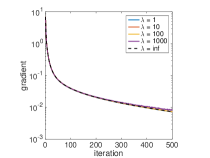
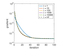
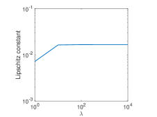
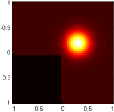
In this example, we consider an L-shaped domain with a source $q$ shaped like a Gaussian bell, as depicted in figure 2. Our goal is to get a constant distribution $y_{d}=1$ in the entire domain. The solution for $u=1$ is shown in figure 3 (a). To solve the optimization problem we use a steepest-descent method with a fixed step-size, determined from the Lipschitz constant of the gradient. The result of the constrained formulation is shown in figure 3 (b). We see that by adapting the boundary conditions we get a more even distribution. The convergence behavior for various values of $\lambda$ is shown in figure 4 (a). We see that as $\lambda\uparrow\infty$, the behaviour tends towards that of the constrained formulation, as expected. The Lipschitz constant of the gradient (evaluated at the initial point $u$), as a function of $\lambda$ is shown in figure 4 (b); the curve levels off as the theory predicts.

Figure 2: L-shaped domain with the source function $q$.

(a)

(b)

Figure 3: Boundary values, $u$, and solution in the interior for the initial and optimized boundary values are depicted in (a) and (b) respectively.

(a)	(b)

Figure 4: The convergence plots for various values of $\lambda$ are depicted in (a), while (b) shows the dependence of the (numerically computed) Lipschitz constant on $\lambda$.

III-B Optimal transport

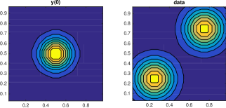
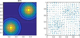
Figure 5: The initial (left) and desired (right) mass density are shown.

Figure 6: The mass density obtained after optimization (left) and the corresponding time-averaged flow field (right) are shown.

(a)	(b)

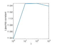
Figure 7: Convergence plots for various values of $\lambda$ are shown in (a), while (b) shows the (numerically computed) Lipschitz constant as a function of $\lambda$.

The second class of PDE-constrained problems we consider comes from optimal transport, where the goal is to determine a mapping, or flow, that optimally transforms one mass density function into another. Say we have two density functions $y_{0}(x)$ and $y_{T}(x)$, with $x\in\Omega$, we can formulate the problem as finding a flowfield, $u(t,x)=\left(\begin{matrix}u_{1}(t,x)\\ u_{2}(t,x)\end{matrix}\right)$, such that $y_{T}(x)=y(T,x)$ and $y_{0}(x)=y(0,x)$, where $y(t,x)$ solves

$$y_{t}+\nabla\cdot(yu)=0.$$

Discretizing using an implicit Lax-Friedrichs scheme [12], the PDE reads

$$A(u)y=q,$$

where $q$ contains the initial condition and we have

$$\small A(u)=\left(\begin{matrix}I+\Delta tB(u^{1})&&&\\ -M&I+\Delta tB(u^{2})&&\\ &-M&&\\ &&&\\ &&-M&I+\Delta tB(u^{N})\\ \end{matrix}\right),$$

with $M$ a four-point averaging matrix and $B$ containing the discretization of the derivative terms. Adding regularization to promote smoothness of $u$ and $y$ in time [12], we obtain the problem

$$\min_{u,y}~{}\textstyle{\frac{1}{2}}\|Py-y_{T}\|_{2}^{2}+\textstyle{\frac{\alpha^{2}}{2}}y^{T}L\mathsf{diag}(u)u$$ (11)

$$\textrm{subject to}\qquad A(u)y=q.$$

Here, $P$ restricts the solution $y$ to $t=T$, $\alpha$ is a regularization parameter and $L$ is a block matrix with $I$ on the main and upper diagonal. The penalized formulation is

$$\min_{u,y}~{}\textstyle{\frac{1}{2}}\|Py-y_{T}\|_{2}^{2}+\textstyle{\frac{\alpha^{2}}{2}}y^{T}L\mathsf{diag}(u)u+\frac{1}{2}\lambda\|A(u)y-q\|^{2}.$$ (12)

Again the partial minimization in $y$ amount to minimizing a quadratic function.

III-B1 Numerical experiments

For the numerical example we consider the domain $\Omega=[0,1]^{2}$, discretized with $\Delta x=1/16$ and $T=1/32$ with a stepsize of $\Delta t=1/8$. The initial and desired state are depicted in figure 5. The resulting state obtained at time $T$ and the corresponding time-averaged flowfield are depicted in figure 6. The initial flow $u_{0}$ was generated by i.i.d. samples from a standard Gaussian random variable. To minimize (12), we used a steepest-descent method with constant step size, using the largest eigenvalue of the Gauss-Newton Hessian at the initial $u$ as an estimate of the Lipschitz constant. The convergence behavior for various values of $\lambda$ as well as the corresponding estimates of the Lipschitz constant at the final solution are shown in figure 7.

Figure 8: Left: Densities, Gaussian (black dash), Huber (red solid), and Student’s t (blue dot). Right: Negative Log Likelihoods.

III-C Robust dynamic inference with the penalty method

In many settings, data is naturally very noisy, and a lot of effort must be spent in pre-processing and cleaning before applying standard inversion techniques.

To narrow the scope, consider dynamic inference, where we wish to infer both hidden states and unknown parameters driven by an underlying ODE. Recent efforts have focused on developing inference formulations that are robust to outliers in the data [3, 9, 4], using convex penalties such as $\ell_{1}$, Huber [14] and non-convex penalties such as the Student’s t log likelihood in place of the least squares penalty. The goal is to develop formulations and estimators that achieve adequate performance when faced with outliers; these may arise either as gross measurement errors, or real-world events that are not modeled by the dynamics.

Figure 8 shows the probability density functions and penalties corresponding to Gaussian, Huber, and Student’s t densities. Quadratic tail growth corresponds to extreme decay of the Gaussian density for large inputs, and linear growth of the influence of any measurement on the fit. In contrast, Huber and Student’s t have linear and sublinear tail growth, respectively, which ensures every observation has bounded influence.

We focus on the Huber function [14], since it is both $C^{1}$-smooth and convex. In particular, the function $f(y)$ in (1) and (4) is chosen to be a composition of the Huber with an observation model. Note that Huber is not $C^{2}$, so this case is not immediately captured by the theory we propose. However, Huber can be closely approximated by a $C^{2}$ function [8], and then the theory fully applies. For our numerical examples, we apply the algorithm developed in this paper directly to the Huber formulation.

We illustrate robust modeling using a simple representative example. Consider a 2-dimensional oscillator, governed by the following equations:

$$\begin{bmatrix}y_{1}\\ y_{2}\end{bmatrix}^{\prime}=\begin{bmatrix}-2u_{1}u_{2}&-u_{1}^{2}\\ 1&0\end{bmatrix}\begin{bmatrix}y_{1}\\ y_{2}\end{bmatrix}+\begin{bmatrix}\sin(\omega t)\\ 0\end{bmatrix}$$ (13)

where we can interpret $u_{1}$ as the frequency, and $u_{2}$ is the damping. Discretizing in time, we have

$$\begin{bmatrix}y_{1}\\ y_{2}\end{bmatrix}^{k+1}=\begin{bmatrix}1-2\Delta tu_{1}u_{2}&-\Delta tu_{1}^{2}\\ \Delta t&1\end{bmatrix}\begin{bmatrix}y_{1}\\ y_{2}\end{bmatrix}^{k}+\Delta t\begin{bmatrix}\sin(\omega t_{k})\\ 0\end{bmatrix}.$$

We now consider direct observations of the second component,

$$z_{k}=\begin{bmatrix}0&1\end{bmatrix}\begin{bmatrix}y_{1}\\ y_{2}\end{bmatrix}^{k}+w_{k},\quad w_{k}\sim N(0,R_{k}).$$

We can formulate the joint inference problem on states and measurements as follows:

$$\min_{u,y}~{}\phi(u,y):=\frac{1}{2}\rho\left(R^{-1/2}(Hy-z)\right)\;\;\mbox{s.t.}\;\;Gy=v,$$ (14)

with $v_{k}=\sin(\omega t_{k})$, $v_{1}$ the initial condition for $y$, and $\rho$ is either the least squares or Huber penalty, and we use the following definitions:

$$\begin{aligned} R&=\mathrm{diag}(\{R_{k}\})\\ H&=\mathrm{diag}(\{H_{k}\})\end{aligned}\quad\begin{aligned} y&=\mathrm{vec}(\{y_{k}\})\\ z&=\mathrm{vec}(\{z_{1},\dots,z_{N}\})\\ G&=\begin{bmatrix}\mathrm{I}&0&&\\ -G_{2}&\mathrm{I}&\ddots&\\ &\ddots&\ddots&0\\ &&-G_{N}&\mathrm{I}\end{bmatrix}\end{aligned}$$

Note in particular that there are only two unknown parameters, i.e. $u\in\mathbb{R}^{2}$, while the state $y$ lies in $\mathbb{R}^{2N}$, with $N$ the number of modeled time points.

The reduced optimization problem for $u$ is given by

$$\min_{u}f(u):=\frac{1}{2}\rho(R^{-1/2}(HG(u)^{-1}v-z).$$

To compute the derivative of the ODE-constrained problem, we can use the adjoint state method. Defining the Lagrangian

$$\mathcal{L}(y,x,u)=\frac{1}{2}\rho\left(R^{-1/2}(Hy-z)\right)+\langle x,Gy-v\rangle,$$

we write down the optimality conditions $\nabla\mathcal{L}=0$ and obtain

$$\left\{\begin{aligned} \overline{y}&=G^{-1}v\\ \overline{x}&=-G^{-T}(H^{T}R^{-1/2}\nabla\rho(R^{-1/2}HG^{-1}v-z))\\ \nabla_{u}f&=\left\langle\overline{x},\frac{\partial(G(u)\overline{y})}{\partial u}\right\rangle\end{aligned}\right\}.$$

The inexact (penalized) problem is given by

$$\min_{u,y}~{}\varphi(u,y)=\frac{1}{2}\rho\left(R^{-1/2}(Hy-z)\right)+\frac{\lambda}{2}\|Gy-v\|^{2}.$$ (15)

We then immediately find

$$\overline{y} =\arg\min_{y}\frac{1}{2}\rho\left(R^{-1/2}(Hy-z)\right)+\frac{\lambda}{2}\|Gy-v\|^{2}$$

$$\nabla\widetilde{\phi}(u) =\lambda\frac{\partial(G(u)\overline{y})}{\partial u}(G\overline{y}-v).$$

When $\rho$ is the least squares penalty, $\overline{y}$ is available in closed form. However, when $\rho$ is the Huber, $\overline{y}$ requires an iterative algorithm. Rather than solving for $\overline{y}$ using a first-order method, we use IPsolve, an interior point method well suited for Huber [5]. Even though each iteration requires inversions of systems of size $\mathcal{O}(N)$, these systems are very sparse, and the complexity of each iteration to compute $\overline{y}$ is $\mathcal{O}(N)$ for any piecewise linear quadratic function [5]. Once again, we see that the computational cost does not scale with $\lambda$.

III-C1 Numerical Experiments

We simulate a data contamination scenario by solving the ODE (13) for the particular parameter value $u=(2,0.1)$. The second component of the resulting state $y$ is observed, and the observations are contaminated. In particular, in addition to Gaussian noise with standard deviation $\sigma=0.1$, for 10% of the measurements uniformly distributed errors in $[0,2]$ are added. The state $y\in\mathbb{R}^{2(4000)}$ is finely sampled over 40 periods.

For the least squares and the Huber penalty with $\kappa=0.1$, we solved both the ODE constrained problem (14) and the penalized version (15) for $\lambda\in\{10^{3},10^{5},10^{7},10^{9}\}$. The results are presented in Table I. The Huber formulation behaves analogously to the formulation using least squares; in particular the outer (projected) function in $u$ is no more difficult to minimize. And, as expected, the robust Huber penalty finds the correct values for the parameters.

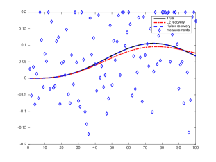
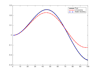
A state estimate generated from $u$-estimates corresponding to large $\lambda$ is shown in Figure 9. The huberized approach is able to ignore the outliers, and recover both better estimates of the underlying dynamics parameters $u$, and the true observed and hidden components of the state $y$.

TABLE I: Results for Kalman experiment. Penalty method for both least squares and huber achieves the same results for moderate values of $\lambda$ as does the projected formulation. While Huber results converge to nearly the true parameters $u$, least squares results converge to an incorrect parameter estimate.

$\lambda$	$\rho$	Iter	Opt	$u$
$10^{3}$	$\ell_{2}$	9	$3.1\times 10^{-7}$	$(.45,.98)$
$10^{5}$	$\ell_{2}$	18	$3.2\times 10^{-7}$	$(.15,4.3)$
$10^{7}$	$\ell_{2}$	26	$5\times 10^{-5}$	$(.07,11.1)$
$10^{9}$	$\ell_{2}$	31	$4\times 10^{-6}$	$(.07,11.8)$
$\infty$	$\ell_{2}$	29	$3.3\times 10^{-7}$	$(.07,11.8)$
$10^{3}$	h	9	$2.4\times 10^{-7}$	$(1.92.14)$
$10^{5}$	h	12	$5\times 10^{-6}$	$(1.98,.11)$
$10^{7}$	h	10	$5\times 10^{-6}$	$(1.99,.11)$
$10^{9}$	h	13	$1\times 10^{-5}$	$(1.99,.11)$
$\infty$	h	17	$2\times 10^{-6}$	$(1.99,.11)$

Figure 9: Top panel: first 100 samples of state $y_{2}$ (solid black), least squares recovery (red dash-dot) and huber recovery (blue dash). Noisy measurements $z$ appear as blue diamonds on the plot, with outliers shown at the top of the panel. Bottom panel: first 100 samples of state $y_{1}$ (solid black), least squares recovery (red dash-dot) and Huber recovery (blue dash).

IV Conclusions

In this paper, we showed that, contrary to conventional wisdom, the quadratic penalty technique can be used effectively for control and PDE constrained optimization problems, if done correctly. In particular, when combined with the partial minimization technique, we showed that the penalized projected scheme

$$\min_{u}~{}g(u)+\min_{y}\left\{f(y)+\frac{\lambda}{2}\|A(u)y-b\|^{2}\right\}$$

has the following advantages:

1. The Lipschitz constant of the gradient of the outer function in $u$ is bounded as $\lambda\uparrow\infty$, and hence we can effectively analyze the global convergence of first-order methods.

2. Convergence behavior of the data-regularized convex inner problem is controlled by parametric matrix $A(\cdot)$, a fundamental quantity that does not depend on $\lambda$.

3. The inner problem can be solved inexactly, and in this case, the number of inner iterations (of a first-order algorithm) needs to grow only logarithmically with $\lambda$ and the outer iterations counter, to preserve the natural rate of gradient descent.

As an immediate application, we extended the penalty method in [22] to convex robust formulations, using the Huber penalty composed with a linear model as the function $f(y)$. Numerical results illustrated the overall approach, including convergence behavior of the penalized projected scheme, as well as modeling advantages of robust penalized formulations.

Acknowledgment. Research of A. Aravkin was partially supported by the Washington Research Foundation Data Science Professorship. Research of D. Drusvyatskiy was partially supported by the AFOSR YIP award FA9550-15-1-0237. The research of T. van Leeuwen was in part financially supported by the Netherlands Organisation of Scientific Research (NWO) as part of research programme 613.009.032.

References

• [1] L. Ambrosio and N. Gigli. A User’s Guide to Optimal Transport. In Modelling and Optimisation of Flows on Networks, pages 1–155. Springer, 2013.
• [2] B. D. Anderson and J. B. Moore. Optimal filtering. 1979, 1979.
• [3] A. Aravkin, B. Bell, J. Burke, and G. Pillonetto. An 1subscript1\ell_{1}-Laplace robust Kalman smoother. IEEE Transactions on Automatic Control, 2011.
• [4] A. Aravkin, J. Burke, and G. Pillonetto. Robust and trend-following Student’s t Kalman smoothers. SIAM Journal on Control and Optimization, 52(5):2891–2916, 2014.
• [5] A. Aravkin, J. V. Burke, and G. Pillonetto. Sparse/robust estimation and Kalman smoothing with nonsmooth log-concave densities: Modeling, computation, and theory. Journal of Machine Learning Research, 14:2689–2728, 2013.
• [6] A. Aravkin, M. Friedlander, F. Herrmann, and T. van Leeuwen. Robust inversion, dimensionality reduction, and randomized sampling. Mathematical Programming, 134(1):101–125, 2012.
• [7] A. Y. Aravkin and T. van Leeuwen. Estimating nuisance parameters in inverse problems. Inverse Problems, 28(11):115016, 2012.
• [8] K. P. Bube and R. T. Langan. Hybrid 1/212\ell 1/\ell 2 minimization with applications to tomography. Geophysics, 62(4):1183–1195, 1997.
• [9] S. Farahmand, G. B. Giannakis, and D. Angelosante. Doubly Robust Smoothing of Dynamical Processes via Outlier Sparsity Constraints. IEEE Transactions on Signal Processing, 59:4529–4543, 2011.
• [10] G. Golub and V. Pereyra. Separable nonlinear least squares: the variable projection method and its applications. Inverse Problems, 19(2):R1–R26, Apr. 2003.
• [11] M. Gugat. Control problems with the wave equation. SIAM Journal on Control and Optimization, 48(5):3026–3051, 2009.
• [12] E. Haber and L. Hanson. Model Problems in PDE-Constrained Optimization. Technical report, 2007.
• [13] S. Haker, L. Zhu, A. Tannenbaum, and S. Angenent. Optimal Mass Transport for Registration and Warping. International Journal of Computer Vision, 60(3):225–240, dec 2004.
• [14] P. J. Huber. Robust Statistics. John Wiley and Sons, 2004.
• [15] R. E. Kalman. A New Approach to Linear Filtering and Prediction Problems. Transactions of the AMSE - Journal of Basic Engineering, 82(D):35–45, 1960.
• [16] Y. Nesterov. Introductory lectures on convex optimization, volume 87 of Applied Optimization. Kluwer Academic Publishers, Boston, MA, 2004. A basic course.
• [17] J. Nocedal and S. Wright. Numerical optimization. Springer Series in Operations Research and Financial Engineering. Springer, New York, second edition, 2006.
• [18] C. C. Paige and M. A. Saunders. LSQR: An algorithm for sparse linear equations and sparse least squares. ACM Transactions on Mathematical Software (TOMS), 8(1):43–71, 1982.
• [19] P. Philip. Optimal Control and Partial Differential Equations. Technical report, LMU Berlin, 2009.
• [20] R. Rockafellar and R. Wets. Variational Analysis, volume 317. Springer, 1998.
• [21] A. Tarantola. Inverse Problem Theory. SIAM, 2005.
• [22] T. van Leeuwen and F. J. Herrmann. A penalty method for pde-constrained optimization in inverse problems. Inverse Problems, 32(1):015007, 2015.
• [23] J. Virieux and S. Operto. An overview of full-waveform inversion in exploration geophysics. Geophysics, 74(6):WCC1–WCC26, 2009.