Significantly improving stellar mass and radius estimates: A new reference function for the $\Delta\nu$ scaling relation

Abstract

The scaling relations between global asteroseismic observables and stellar properties are widely used to estimate masses and radii of stars exhibiting solar-like oscillations. Since the mass and radius of the Sun are known independently, the Sun is commonly used as a reference to scale to. However, the validity of the scaling relations depends on the homology between the star under study and the reference star. Solar-like oscillators span a wide range of masses and metallicities, as well as evolutionary phases. Most of these stars are therefore not homologous to the Sun. This leads to errors of up to 10% (5%) in mass (radius) when using the asteroseismic scaling relations with the Sun as the reference. In this paper we derive a reference function to replace the solar-reference value used in the large-frequency-separation scaling relation. Our function is the first that depends on both effective temperature and metallicity, and is applicable from the end of the main sequence to just above the bump on the red giant branch. This reference function improves the estimates of masses and radii determined through scaling relations by a factor of 2, i.e. allows masses and radii to be recovered with an accuracy of 5% and 2%, respectively.

1 Introduction

Mass and radius are the most fundamental among stellar parameters. Knowledge of these parameters not only enables one to characterize a star, but it is also a prerequisite for characterizing planets orbiting a star. Asteroseismic scaling relations are a fast and straightforward method that can be used to estimate masses and radii of stars that exhibit solar-like oscillations. These are low-amplitude oscillations that are excited stochastically by convection in the outer zones of cool stars.

One scaling relation links the so-called large frequency separation, i.e., the frequency difference between modes of the same degree and consecutive radial orders ($\Delta\nu$) to the square root of the stellar mean density (Ulrich, 1986).

$${\Delta\nu}\propto\sqrt{\frac{M}{R^{3}}},$$ (1)

where $R$ and $M$ are the stellar radius and mass. The constant of proportionality is determined using $\Delta\nu$ for the Sun, $\Delta\nu_{\odot}=135.1\pm 0.1\mu$Hz (Huber et al., 2011).

The second scaling relation links the frequency at which the maximum of the oscillation power occurs, $\nu_{\rm max}$, with stellar properties. Based on the argument by Brown et al. (1991) that $\nu_{\rm max}$ should scale with the acoustic cutoff frequency $\nu_{\rm ac}$, Kjeldsen & Bedding (1995) formulated the $\nu_{\rm max}$ scaling relation.

$$\nu_{\rm{max}}\propto\frac{M}{R^{2}\sqrt{T_{\rm{eff}}}}.$$ (2)

Again, the constant of proportionality is determined using the solar value of $\nu_{\rm max}$ as reference: $\nu_{\rm{max},\odot}=3050$ (Kjeldsen & Bedding, 1995), and $T_{\rm{eff},\odot}=5772$ K (Mamajek et al., 2015).

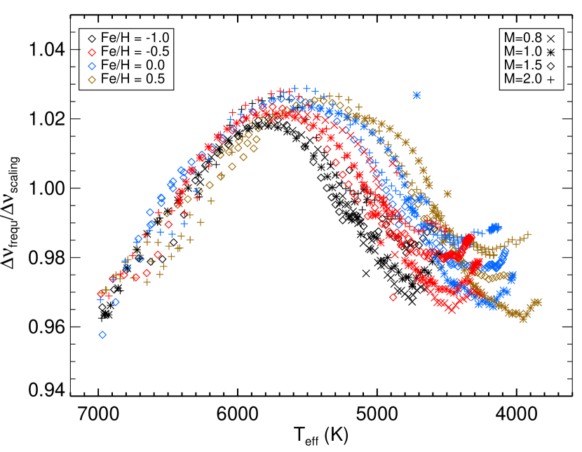
The accuracy of the stellar radii obtained from scaling relations has been tested through comparisons with radii obtained from independent measurements such as interferometry. These estimates are in good agreement within uncertainties, which can be about 10% for interferometric radii of red giants due to uncertainties in the parallaxes (Huber et al., 2012). However, the differences in structure between the Sun and the stars investigated result in inherent systematic deviations of the values computed with the scaling relations with respect to the true values. The underlying physical reason of the $\Delta\nu$ relation is understood. Hence, we can compute the deviation of $\Delta\nu$ from the scaling relation with respect to the $\Delta\nu$ value obtained from individual frequencies (see Fig. 1). The influence of $\nu_{\rm max}$ on the $\Delta\nu$ scaling relation can currently not be studied through comparisons with models because $\nu_{\rm max}$ can currently not be calculated theoretically.

Using the $\Delta\nu$ scaling relation with a fixed reference value results in masses and radii with an intrinsic error of about 10 and 5 percent, respectively.

1.1 Mismatches and earlier corrections

In their study of a planet-hosting red-giant star Huber et al. (2013) noticed that results from grid-based modeling using the scaling relations indicated in Eqs 1 and 2 and the solar reference differ by 5% from those based on the modeling of individual frequencies. Mismatches for non-solar metallicities are also known: in their sample of metal-poor stars (-2.3 dex < [M/H] < -1.0 dex) Epstein et al. (2014) found masses derived from scaling relations to be systematically higher than expected from other astrophysical priors.

Efforts have been made by several groups to improve the accuracy of the scaling relations. Belkacem et al. (2013) and Mosser et al. (2013) argued that observations are often only possible far from the asymptotic regime, i.e., at too low radial orders to justify the asymptotic approximation. Therefore they suggested to use the second order effects in the large frequency separation to derive asymptotic spacings from the observations. It was then shown by Hekker et al. (2013) that the postulated discrepancies from the asymptotic behaviour have most likely been overestimated. Miglio et al. (2012) suggested a correction factor of 2.7 percent for the radius of stars in the red clump. This correction factor was derived based on the fact that two models with the same mass and radius show a significant difference in $\Delta\nu$ depending on their evolutionary state. This difference in $\Delta\nu$ between red-clump stars and red giant branch stars is due to differences in the sound-speed profile. A different approach was taken by White et al. (2011) who proposed a quadratic correction function $f(T_{\rm{eff}})$ that was calibrated with $\Delta\nu$ values derived from the pulsation frequencies of stellar models, in particular with models constructed with the ASTEC code (Christensen-Dalsgaard, 2008). Their correction is applicable from the main-sequence to temperatures down to 4700K which includes sub giants and red giants up to near the RGB bump depending on mass and metallicity. As can be seen from Fig. 1, the deviation from the scaling relation cannot be represented as a quadratic function for temperatures below this limit, which correspond to temperatures of many of the observed red giants. Additionally, the correction was only calibrated for stars with near-solar metallicities, and no [Fe/H] dependence is included in their formulation. Given the astrophysical importance of cool red-giant stars and the fact that many stars have metallicities outside the range of the models on which the previous correction was based (the metallicities used were Z=0.011, Z=0.017 and Z=0.028, corresponding to [Fe/H] values of -0.19, 0.0, and 0.21), our goal is to determine a reference function that works for red giants, and that can be applied to stars in a wider range of metallicities. Recently another approach has been suggested by Sharma et al. (2016) which relies on interpolation in a grid of models. This method however requires the use of grids of models, while we present here a method that can be straightforwardly applied.

Figure 1: Ratio of $\Delta\nu$ derived from individual frequencies to $\Delta\nu$ determined using the $\Delta\nu$ scaling relation (Eq. 1) with a solar reference value. Different metallicities are shown in different colors, and different masses with different symbols (see legends). The horizontal dashed line indicates a ratio of 1.

Figure 2: Hertzsprung-Russell diagram of the YREC models used in this study. Different metallicities are shown in different colors (see legend), while masses are indicated in different line styles (solid: M=2 M_⊙, dotted: M=1.5 M_⊙, dashed: M=1 M_⊙, dash-dotted M=0.8 M_⊙). The models actually used in this study (see Section 3.1) are indicated with thick lines.

2 Models

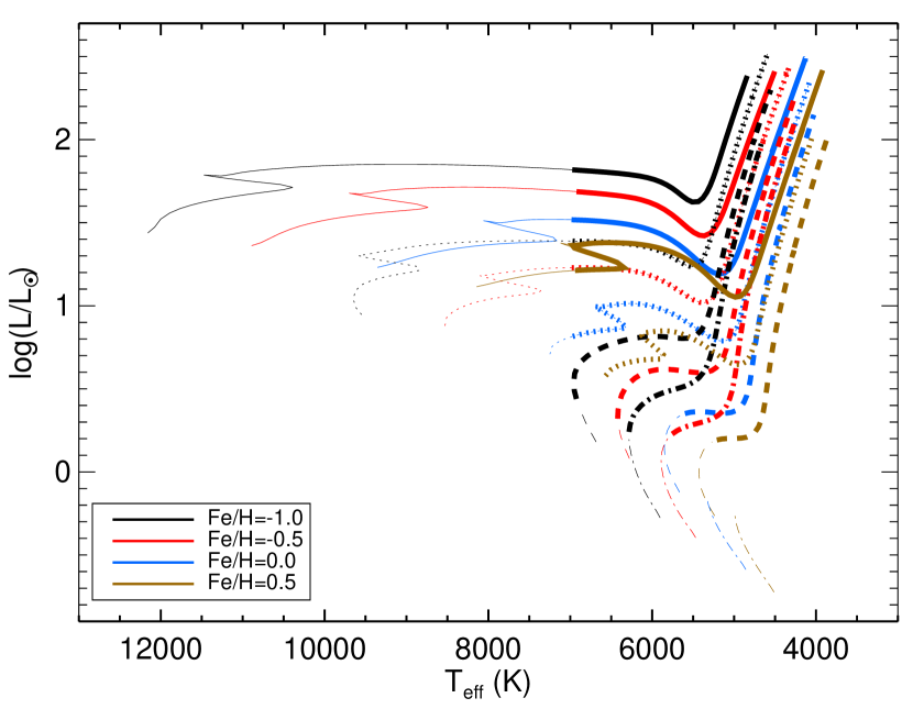
We used models computed with the YREC stellar evolution code (Demarque et al., 2008). Models were computed using OPAL opacities (Iglesias & Rogers, 1996) supplemented with low temperature (log T < 4.1) opacities of Ferguson et al. (2005) and the OPAL equation of state (Rogers & Nayfonov, 2002). All nuclear reaction rates are obtained from Adelberger et al. (1998), except for that of the ${}^{14}N(p,\gamma)^{15}O$ reaction, for which we use the rate of Formicola et al. (2004). We computed models with masses of 0.8, 1.0, 1.5, and 2.0 M_⊙, and metallicities of $-1.0$, $-0.5$, $0.0$, and $0.5$ dex. Although this is a coarser grid than used by Sharma et al. (2016) we deem this sufficient based on the monotonic behavior of the models with metallicity. Evolution was followed from the main sequence to slightly beyond the bump on the red-giant branch. We included models with $\nu_{\rm max}$ > 6 $\mu$ Hz. See Fig. 2 for a Hertzsprung-Russell diagram showing the model tracks. All models described here were constructed with the Eddington $T-\tau$ relation in their atmosphere. To study the effect of atmospheric structure, we use two sequences of solar metallicity and masses of $M$=1.0; 1.2 M_⊙ models constructed with the Krishna Swamy $T-\tau$ relation (Krishna Swamy, 1966), where the $M$=1.0 M_⊙ sequence also has a slightly different mixing length parameter.

2.1 Calculating $\Delta\nu$

We derive $\Delta\nu$ from the computed oscillation radial-mode frequencies of the models. Since frequencies of any order can be computed, including those orders that are not observed, we use only a subset of the modes. We selected modes around the value of $\nu_{\rm max}$. The value of $\nu_{\rm max}$ was computed for each model from the known mass, temperature and radius using Eq. 2 with $\nu_{\rm max,\odot}=3050~{}\mu$Hz (Kjeldsen & Bedding, 1995); $\Delta\nu$ was then determined by a weighted linear fit to the frequencies versus the radial order. This is similar to the method of White et al. (2011). However, we used a different width of the weighting function. The weights were set using a Gaussian centered at $\nu_{\rm max}$ with a height of 1 and a full-width at half maximum set to $5\Delta\nu$. The width is defined empirically and taken such that it is applicable over a wide parameter space to include enough frequencies to determine $\Delta\nu$ and to resemble the number of radial modes typically observed. For red giants this width is consistent with the observed FWHM of $(0.66\pm 0.01)\nu_{\rm max}^{0.88\pm 0.01}$ (Mosser et al., 2012). Our definition of the width of the weighting function leads to a wider gaussian on the red giant branch compared to the definition FWHM=$0.25\cdot\nu_{max}$ which was used by White et al. (2011). The $\Delta\nu$ value used to determine the width of the Gaussian function is computed using Eq. 1 with $\Delta\nu_{\odot}=135~{}\mu$Hz. It was shown by Hekker et al. (2013) that the $\Delta\nu$ values of Kepler red giants derived from the radial modes do not differ significantly from the values obtained from the power spectrum of the power spectrum (see their Fig. 1). It is therefore safe to assume that our method provides a good estimate of $\Delta\nu$ even when mixed modes are present in the power spectrum.

As a Gaussian weighting function assigns non-zero weights even at frequencies far away from its centre, it could include signal from above the acoustic cutoff frequency $\nu_{\rm ac}$  if oscillations are computed in that regime. To mitigate this, the dimensionless value of the normalized weighting function at $\nu_{\rm ac}$ was subtracted from the weighting function so that it was shifted downwards to become zero at $\nu_{\rm ac}$. Shifts were small ($10^{-9}$ to $10^{-5}$) on the main sequence and larger (up to 0.5) on the red-giant branch. Negative values of the shifted weighting function were set to zero.

We note that we do not have a calibrated solar model in our set. Our most solar like model has a $\Delta\nu$ value of 136.1 $\mu$Hz. The offset between the observed solar value and this value is most likely due to surface effects that cannot be incorporated directly in the current analysis.

3 A metallicity dependent reference function

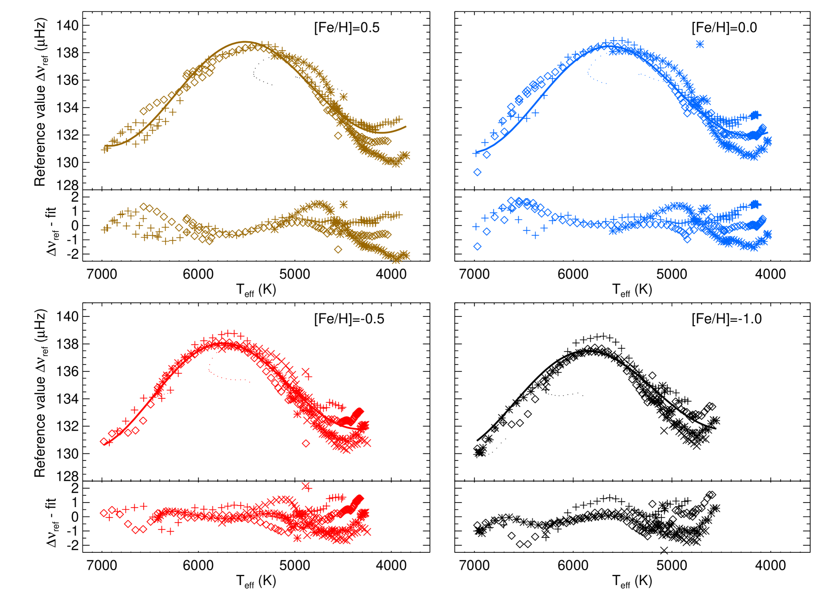
From $\Delta\nu$ computed as described above, and the known mass and radius of the model it is possible to compute the value that $\Delta\nu_{\odot}$ should have for each model to reproduce the correct mean density. We call this $\Delta\nu_{\rm ref}$. These values, for our set of YREC models, are plotted in Fig. 3 as a function of $T_{\rm eff}$. The reference values as a function of $T_{\rm eff}$ take the shape of one half of a sinusoid with a decreasing amplitude. Hence, we fitted a damped sinusoid using a Levenberg-Marquardt least-squares minimization. We then iteratively changed the coefficients of the damped sinusoid to depend on [Fe/H]. This results in the following fit:

$$\Delta\nu_{\rm{ref}}=\rm{A}\cdot e^{\lambda\rm{T_{eff}}/10^{4}K}\cdot(\cos(\omega\cdot\rm{T_{eff}}/10^{4}K+\phi))+B$$ (3)

Parameters $A$, $\lambda$, $\omega$, $\phi$, and $B$ of equation 3 are listed in Table 1. This function (Eq. 3) should be used instead of $\Delta\nu_{\odot}$ to take $T_{\rm eff}$ and [Fe/H] effects into account in the scaling relations. The residuals between the reference values for each model and Eq. 3 are shown in the lower sub-panel of each of the four panels in Fig. 3. These residuals still show a dependence on mass, which will be addressed in a forthcoming paper.

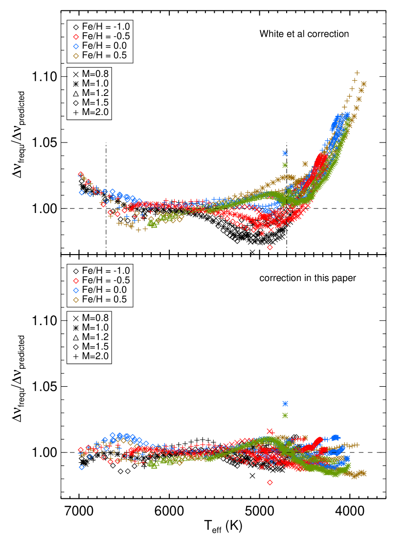
The robustness of this fit was examined using a Monte-Carlo approach in which we perturbed the model input values 10 000 times assuming typical uncertainties of 80 K in temperature, 1% in $\Delta\nu$ and 0.1 dex in [Fe/H] (Davies et al., 2016). A new fit was computed for each realisation. The maximum deviation between fits, calculated by dividing the fits, is typically 0.44% with a standard deviation of 0.16%, i.e. nearly an order of magnitude smaller than the effect we aim to correct (see Fig. 1). Finally, $\Delta\nu_{\rm ref}$ computed for the models with the Krishna Swamy $T-\tau$ relation are in line with the values for the other models (see Fig. 4).

Figure 3: Each panel shows the reference values with the reference function (solid line) for one metallicity in the top part with residuals in the bottom part. The small dots indicate the models that have not been included in the current analysis (see text for more details). The residual value of the outlier in [Fe/H] = 0.0 at $T_{\rm eff}\approx 4700$ K is off the scale and not shown.

3.1 Parameter range of the validity of the reference function

The models that are incorporated in this study are shown with thick lines in Fig. 2. Low-mass (M=0.8 and M=1.0) models on the beginning of the main-sequence do not follow the general trend of the other models. These models create loops in $\Delta\nu_{\rm ref}$–$T_{\rm eff}$ relation (shown as small dots in Fig. 3) and we excluded them from our current analysis. Models with $T_{\rm{eff}}>7000$ K were also excluded as such high-temperature stars will not have an outer convection zone deep enough to excite oscillations. These two cuts left the end of the main sequence in the sample, while removing the early main sequence phases. We note that most oscillating MS stars are observed in the later phases due to biases in the photometric observations of solar-like oscillations towards hotter and more evolved stars on the MS (Chaplin et al., 2011). Our models go down to $\nu_{\rm max}$ = 6 $\mu$Hz which occurs at $T_{\rm eff}$ between 3800 K and 4500 K, depending on [Fe/H] and mass.

We note that there are a few models that have reference values that deviate from the general trend (see Fig. 1 and 3). We currently do not know the reason for these deviations. One possibility is that this is related to the luminosity bump.

Table 1: Parameters of the correction function.

A	0.64[Fe/H] + 1.78 $\mu Hz$
$\lambda$	$-$0.55[Fe/H] + 1.23
$\omega$	22.21 rad/K
$\phi$	0.48[Fe/H] + 0.12
B	0.66[Fe/H] + 134.92 $\mu Hz$

3.2 Comparison of reference functions

To justify the inclusion of a metallicity dependence in the reference function we show that this a significant improvement in the derived stellar mean densities (and thus masses and radii) using scaling relations. To do this, we compare the performance of our $T_{\rm eff}$ and [Fe/H]-dependent reference function with the quadratic function proposed by White et al. (2011) that only depends on $T_{\rm eff}$. We visualize the differences in the top panel of Fig. 4. The previously available correction works well in its defined range and for solar metallicity. However, for other metallicities systematic biases occur around 5000K. We mitigate these biases in this work, and at the same time we extend the range in which the reference works by about 1000K. This is about half of the previously available range. Additionally, we quantify the performance of the corrections by using a cross-validation technique: we fit our function and the quadratic temperature function of White et al. (2011) 10 times, each time 10% of the models were randomly excluded from the procedure. We then predict the mean density of the excluded models and compare the predicted values with the real values using the coefficient of determination which is a goodness-of-fit measure defined as

$$R^{2}\equiv 1-\frac{\sum_{i}(y_{i}-f_{i})^{2}}{\sum_{i}(y_{i}-\bar{y})^{2}},$$ (4)

where $y_{i}$ indicate the individual ‘observed’ data points, $\bar{y}$ indicates the mean of the observed data and $f_{i}$ indicates the predicted value (Weihs et al., 2013). This test is the standard method for model selection and evaluation in statistics. It evaluates how well our model is able to predict unseen values as opposed to describing values that have been fitted for. A value of $R^{2}=1$ means a perfect fit, while a $R^{2}=0$ indicates that the fit does not reduce the variance. For the reference function derived in this work we find a value of $R^{2}=0.88$. This value is the same both for the whole parameter space investigated in this work, as well as for the temperature range for which the quadratic function of White et al. (2011) was developed, i.e. 6700K $\geq\rm{T}_{\rm{eff}}\geq$4700K. The $R^{2}$ value for the quadratic function recalibrated to our [Fe/H]=0 YREC models is 0.54 when applied to all metallicities.

We note that the correction proposed by White et al. (2011) and the one recalibrated to YREC models showed differences smaller than 0.5%, indicating that differences in stellar evolution codes (at least between YREC and ASTEC in the relevant $T_{\rm eff}$ range) introduce a deviation of the same order as the uncertainties in the measurements (see Section 3), which are significantly smaller than the corrections to the $\Delta\nu$ scaling relation suggested by White et al. (2011) and in this work.

4 Conclusions

Figure 4: Same as Fig. 1 but now using the scaling relation (Eq. 1) with corrections. The top panel uses the correction by White et al. (2011). Vertical lines indicate the temperature range for which this correction function is valid. The bottom panel shows the result using the method proposed in this work where a reference function (Eq. 3) is used instead of the solar reference value. The ratio for the models with the Krishna Swamy (KS) $T-\tau$ relation are indicated in green.

We have developed a new reference function for use with the asteroseismic scaling relation linking $\Delta\nu$ to the stellar mean density (Eq. 1). This reference function includes dependencies on $T_{\rm eff}$ and [Fe/H] and increases the accuracy of masses and radii determined using the scaling relations by a factor of 2. It can immediately be used to estimate more accurate masses and radii for the ten thousands of stars for which solar-like oscillations have been observed by CoRot (Baglin et al., 2006), Kepler (Borucki et al., 2008) and K2 (Haas et al., 2014) and that are currently being studied. Additionally, this can be applied to the many oscillators expected to be observed by missions such as TESS (Ricker et al., 2015) and Plato (Rauer et al., 2014). While this functional form cannot fully capture the complex behavior of the $\Delta\nu$ deviations it has the advantage that it can be applied in a straightforward manner – even without using grid-based modeling – to extract masses and radii. Furthermore, it can also be used with existing grids that do not have oscillations computed.

This is the first reference function that takes metallicity (-1.0 dex $\leq$ Fe/H $\leq$ 0.5 dex) into account. This function is applicable to stars in different evolutionary states including (end of) main-sequence stars, subgiants and cool red giant stars down to $\nu_{\rm max}$ = 6 $\mu$Hz, with the exception of low-mass main-sequence stars and red-clump stars. Uncertainties in the data and differences in stellar evolution codes and model atmospheres impact the reference function at a level that is an order of magnitude smaller than the proposed improvement to the $\Delta\nu$ scaling relation. Hence, we consider the reference function proposed in this work to be widely applicable, i.e. to both models and observed data. A mass dependence still remains, especially on the red giant branch. This will be addressed in a forthcoming paper.

References

- Adelberger et al. (1998) Adelberger E. G., et al., 1998, Reviews of Modern Physics, 70, 1265
- Baglin et al. (2006) Baglin A., Auvergne M., Barge P., Deleuil M., Catala C., Michel E., Weiss W., COROT Team 2006, in Fridlund M., Baglin A., Lochard J., Conroy L., eds, ESA Special Publication Vol. 1306, The CoRoT Mission Pre-Launch Status - Stellar Seismology and Planet Finding. p. 33
- Belkacem et al. (2013) Belkacem K., Samadi R., Mosser B., Goupil M.-J., Ludwig H.-G., 2013, in Shibahashi H., Lynas-Gray A. E., eds, Astronomical Society of the Pacific Conference Series Vol. 479, Progress in Physics of the Sun and Stars: A New Era in Helio- and Asteroseismology. p. 61 (arXiv:1307.3132)
- Borucki et al. (2008) Borucki W., et al., 2008, in Sun Y.-S., Ferraz-Mello S., Zhou J.-L., eds, IAU Symposium Vol. 249, Exoplanets: Detection, Formation and Dynamics. pp 17–24, doi:10.1017/S174392130801630X
- Brown et al. (1991) Brown T. M., Gilliland R. L., Noyes R. W., Ramsey L. W., 1991, ApJ, 368, 599
- Chaplin et al. (2011) Chaplin W. J., et al., 2011, Science, 332, 213
- Christensen-Dalsgaard (2008) Christensen-Dalsgaard J., 2008, Ap&SS, 316, 13
- Davies et al. (2016) Davies G. R., et al., 2016, MNRAS, 456, 2183
- Demarque et al. (2008) Demarque P., Guenther D. B., Li L. H., Mazumdar A., Straka C. W., 2008, Ap&SS, 316, 31
- Epstein et al. (2014) Epstein C. R., et al., 2014, ApJ, 785, L28
- Ferguson et al. (2005) Ferguson J. W., Alexander D. R., Allard F., Barman T., Bodnarik J. G., Hauschildt P. H., Heffner-Wong A., Tamanai A., 2005, ApJ, 623, 585
- Formicola et al. (2004) Formicola A., et al., 2004, Physics Letters B, 591, 61
- Haas et al. (2014) Haas M. R., et al., 2014, in American Astronomical Society Meeting Abstracts #223. p. 228.01
- Hekker et al. (2013) Hekker S., Elsworth Y., Basu S., Mazumdar A., Silva Aguirre V., Chaplin W. J., 2013, MNRAS, 434, 1668
- Huber et al. (2011) Huber D., et al., 2011, ApJ, 743, 143
- Huber et al. (2012) Huber D., et al., 2012, ApJ, 760, 32
- Huber et al. (2013) Huber D., et al., 2013, Science, 342, 331
- Iglesias & Rogers (1996) Iglesias C. A., Rogers F. J., 1996, ApJ, 464, 943
- Kjeldsen & Bedding (1995) Kjeldsen H., Bedding T. R., 1995, A&A, 293, 87
- Krishna Swamy (1966) Krishna Swamy K. S., 1966, ApJ, 145, 174
- Mamajek et al. (2015) Mamajek E. E., et al., 2015, preprint, (arXiv:1510.07674)
- Miglio et al. (2012) Miglio A., et al., 2012, MNRAS, 419, 2077
- Mosser et al. (2012) Mosser B., et al., 2012, A&A, 537, A30
- Mosser et al. (2013) Mosser B., et al., 2013, A&A, 550, A126
- Rauer et al. (2014) Rauer H., et al., 2014, Experimental Astronomy, 38, 249
- Ricker et al. (2015) Ricker G. R., et al., 2015, Journal of Astronomical Telescopes, Instruments, and Systems, 1, 014003
- Rogers & Nayfonov (2002) Rogers F. J., Nayfonov A., 2002, ApJ, 576, 1064
- Sharma et al. (2016) Sharma S., Stello D., Bland-Hawthorn J., Huber D., Bedding T. R., 2016, preprint, (arXiv:1603.05661)
- Ulrich (1986) Ulrich R. K., 1986, ApJ, 306, L37
- Weihs et al. (2013) Weihs C., Mersmann O., Ligges U., 2013, Foundations of Statistical Algorithms
- White et al. (2011) White T. R., Bedding T. R., Stello D., Christensen-Dalsgaard J., Huber D., Kjeldsen H., 2011, ApJ, 743, 161