A splitting method for deep water with bathymetry

Afaf Bouharguane Univ. Bordeaux, IMB, INRIA MEMPHIS, UMR 5251, F-33400 Talence, France. afaf.bouharguane@math.u-bordeaux1.fr  and  Benjamin Melinand Univ. Bordeaux, IMB, UMR 5251, F-33400 Talence, France. benjamin.melinand@math.u-bordeaux1.fr
Abstract.

In this paper we derive and prove the wellposedness of a deep water model that generalizes the Saut-Xu system for nonflat bottoms. Then, we present a new numerical method based on a splitting approach for studying this system. The advantage of this method is that it does not require any low pass filter to avoid spurious oscillations. We prove a local error estimate and we show that our scheme represents a good approximation of order one in time. Then, we perform some numerical experiments which confirm our theoretical result and we study three physical phenomena : the evolution of water waves over a rough bottom; the evolution of a KdV soliton when the shallowness parameter increases; the homogenization effect of rapidly varying topographies on water waves.

1. Introduction

1.1. Presentation of the problem

Understanding the influence of the topography on water waves is an important issue in oceanography. Many physical phenomena are linked to the variation of the topography : shoaling, rip currents, diffraction, Bragg reflection. Since the direct study on the Euler equations is quite involved, several authors derived and justified asymptotic models according to different small parameters. A usual way to derive asymptotic models is to start from the Zakharov/Craig-Sulem-Sulem formulation [38, 16, 17], which is a good formulation for irrotational water waves, and to expand the Dirichlet-Neumann operator. Then, in the shallow water regime for example, several models were obtained like the Saint-Venant equations or the Green-Naghdi or Boussinesq equations, see [2, 24], [22] for instance. The present paper addresses the influence of the bathymetry in deep water, in the sense explained below.

In this paper, a𝑎a denotes the typical amplitude of the water waves, L𝐿L the typical length, H𝐻H the typical height and abottsubscript𝑎𝑏𝑜𝑡𝑡a_{bott} the typical amplitude of the bathymetry. Then, we introduce three parameters : ε=aH𝜀𝑎𝐻\varepsilon=\frac{a}{H} the nonlinearity parameter, μ=H2L2𝜇superscript𝐻2superscript𝐿2\mu=\frac{H^{2}}{L^{2}} the shallowness parameter and β=abottH𝛽subscript𝑎𝑏𝑜𝑡𝑡𝐻\beta=\frac{a_{bott}}{H} the bathymetric parameter. We recall that assuming μ𝜇\mu small leads to shallow water models. In deep water, which is typically the case when μ𝜇\mu is of order 111, it is quite common to assume that the steepness parameter εμ=aL𝜀𝜇𝑎𝐿\varepsilon\sqrt{\mu}=\frac{a}{L} is small. The first asymptotic model with a small steepness assumption was derived by Matsuno in 2D for a flat and non-flat bottom and weakly transverse 3D water waves [27, 28]. Then, Choi extended this result in 3D for flat bottom [12]. Finally, Bonneton and Lannes gave a 3D version in the case of a non-flat bottom [8]. It is important to notice that these models are only formally derived. It is proven in [2] that smooth enough solutions to theses models are close to the solutions of the water waves equations but, to the best of our knowledge, the wellposedness of the Mastuno equations, even in the case of a flat bottom, is still an open problem. This system could be illposed (see Ambrose, Bona and Nicholls [3]). To avoid this difficulty, Saut and Xu ([34]) developed an equivalent system to the Matsuno system which is consistent with the water waves problem and with the same accuracy. Then, they proved that this new system is wellposed. However, this model is for a flat bottom. In this paper, we derive (see Section 2), use, and prove the wellposedness of a generalization of the Saut-Xu system with a non-flat bottom which is the following system

(1.1) {tζμv+εμ(12vxζ+12μ(vxμζ)+μ(ζxμv)+ζxv)=βμx(Bμv)tv+xζ+3εμ2vxvεμ2xζμxζεμ2vμ2xv=0,\left\{\begin{aligned} &\partial_{t}\zeta-\mathcal{H}_{\mu}v+\varepsilon\sqrt{\mu}\left(\frac{1}{2}v\partial_{x}\zeta+\frac{1}{2}\mathcal{H}_{\mu}\left(v\partial_{x}\mathcal{H}_{\mu}\zeta\right)+\mathcal{H}_{\mu}\left(\zeta\partial_{x}\mathcal{H}_{\mu}v\right)+\zeta\partial_{x}v\right)=\beta\sqrt{\mu}\partial_{x}\left(B_{\mu}v\right)\\ &\partial_{t}v+\partial_{x}\zeta+\frac{3\varepsilon\sqrt{\mu}}{2}v\partial_{x}v-\frac{\varepsilon\sqrt{\mu}}{2}\partial_{x}\zeta\mathcal{H}_{\mu}\partial_{x}\zeta-\frac{\varepsilon\sqrt{\mu}}{2}v\mathcal{H}_{\mu}^{2}\partial_{x}v=0,\end{aligned}\right.

where (see Subsection 1.2 for the notations)

μ=tanh(μD)Dx and Bμ=sech(μD)(bsech(μD)).\mathcal{H}_{\mu}=-\frac{\tanh(\sqrt{\mu}D)}{D}\partial_{x}\text{ and }B_{\mu}=\text{sech}(\sqrt{\mu}D)\left(b\;\text{sech}(\sqrt{\mu}D)\;\cdot\;\right).

Many authors developed numerical approaches to study the impact of the bottom on water waves, see for instance [29], [25], [36], [18], [10], [30], [20], [6], [7]). However to the best of our knowledge, when one works with deep water, there is no convergence result in the literature. After the original work of Craig and Sulem ([16]) and the paper of Craig et al. ([14]), Guyenne and Nicholls ([19]) developed a numerical method based on a pseudospectral method and a fourth-order Runge-Kutta scheme for the time integration. The linear terms are solved exactly whereas the nonlinear terms are viewed as source terms. Their approach has been developed for the whole water waves equations but we could easily adapt it to our system. However with their scheme, we observe spurious oscillations in the wave profile that lead to instabilities. These errors seem to appear when the nonlinear part is evaluated via the Fourier transform. This is the aliasing phenomenon. Guyenne and Nicholls also observe these oscillations and, to fix it, they apply at every time step a low-pass filter. The scheme that we propose in this paper avoids this low-pass filter.

We present a new numerical method based on a splitting approach for studying nonlinear water waves in the presence of a bottom. We remark that the Saut-Xu system contains a dispersive part and a nonlinear transport part. Thus, the splitting method becomes an interesting alternative to solve the system since this approach is commonly used to split different physical terms, see for instance [32]. We also motivate our decomposition by the fact that, due to the pseudodifferential operator, some terms in the dispersive part may be computed efficiently using the fast Fourier transform. The transport part is computed by a Lax-Wendroff method. Various versions of the splitting method have been developed for instance for the nonlinear Schrodinger, the viscous Burgers equation, Korteweg-de-Vries equations [9, 21, 26, 33, 37]. Thanks to this splitting, we only use a pseudospectral method for the nonlocal terms (contrary to [16, 19]), which limits the aliasing phenomenon and allows us to avoid a low-pass filter.

We denote by ΦtsuperscriptΦ𝑡\Phi^{t} the nonlinear flow associated to the Saut-Xu system (1.1), Φ𝒜tsubscriptsuperscriptΦ𝑡𝒜\Phi^{t}_{\mathcal{A}} and Φ𝒟tsubscriptsuperscriptΦ𝑡𝒟\Phi^{t}_{\mathcal{D}}, respectively, the evolution operator associated with the transport part (see equation (3.1)) and with the dispersive part (see (3.2)). We consider the Lie formula defined by

(1.2) 𝒴t=Φ𝒜tΦ𝒟t.superscript𝒴𝑡subscriptsuperscriptΦ𝑡𝒜subscriptsuperscriptΦ𝑡𝒟\mathcal{Y}^{t}=\Phi^{t}_{\mathcal{A}}\Phi^{t}_{\mathcal{D}}.\\

The Saut-Xu system (1.1) is a quasilinear system. This implies derivatives losses in the proof of the convergence. In Theorem 4.6, we show that the numerical solution converges to the solution of the Saut-Xu system (1.1) in the HN+12×HNsuperscript𝐻𝑁12superscript𝐻𝑁H^{N+\frac{1}{2}}\times H^{N}-norm for initial data in HN+127×HN7()superscript𝐻𝑁127superscript𝐻𝑁7H^{N+\frac{1}{2}-7}\times H^{N-7}(\mathbb{R}), where N7.𝑁7N\geq 7.

Notice that it is not hard to generalize the present work to the Lie formula Φ𝒟tΦ𝒜tsubscriptsuperscriptΦ𝑡𝒟subscriptsuperscriptΦ𝑡𝒜\Phi^{t}_{\mathcal{D}}\Phi^{t}_{\mathcal{A}}. We also make the choice to prove a convergence result for a Lie splitting but our proof can be adapted to a Strang splitting or a more complex one. Finally, notice that our scheme can be used for other equations.

The paper is organised as follows. In the next section, we extend the Saut-Xu system by adding a topography term and we prove a local wellposedness result. We also show that the flow map ΦtsuperscriptΦ𝑡\Phi^{t} is uniformly Lipschitzean. In section 3, we split the problem and we give some estimates on Φ𝒜tsubscriptsuperscriptΦ𝑡𝒜\Phi^{t}_{\mathcal{A}} and Φ𝒟tsubscriptsuperscriptΦ𝑡𝒟\Phi^{t}_{\mathcal{D}}. In Section 4, we prove a local error estimate and we show that the Lie method represents a good approximation of order one in time (Theorem 4.6). Finally, in Section 5, we perform some numerical experiments which confirm our theoretical result and we illustrate three physical phenomena : the evolution of water waves over a rough bottom; the evolution of a KdV soliton when the shallowness parameter increases and the homogenization effect of rapidly varying topographies on water waves.

1.2. Notations and assumptions

  • x𝑥x denotes the horizontal variable and z𝑧z the vertical variable. In this paper, we only study the 2D case (x𝑥x\in\mathbb{R}).

  • We assume that

    (1.3) 0ε,β1μmax>μmin>0μmaxμμmin.formulae-sequence0𝜀𝛽1subscript𝜇subscript𝜇0subscript𝜇𝜇subscript𝜇0\leq\varepsilon,\beta\leq 1\text{, }\exists\mu_{\max}>\mu_{\min}>0\text{, }\mu_{\max}\geq\mu\geq\mu_{\min}.
  • We denote δ=max(ε,β)𝛿𝜀𝛽\delta=\max(\varepsilon,\beta).

  • We denote Λ=(1x2)1/2Λsuperscript1superscriptsubscript𝑥212\Lambda=(1-\partial_{x}^{2})^{1/2} and Hs()={uL2(),uH2=ΛsuL2<}superscript𝐻𝑠formulae-sequence𝑢superscript𝐿2subscriptnorm𝑢superscript𝐻2subscriptnormsuperscriptΛ𝑠𝑢superscript𝐿2H^{s}(\mathbb{R})=\left\{u\in L^{2}(\mathbb{R}),||u||_{H^{2}}=||\Lambda^{s}u||_{L^{2}}<\infty\right\} the usual Sobolev space for s0𝑠0s\geq 0.

  • Let f𝒞0()𝑓superscript𝒞0f\in\mathcal{C}^{0}\left(\mathbb{R}\right) and m𝑚m\in\mathbb{N} such that f1+|x|mL()𝑓1superscript𝑥𝑚superscript𝐿\frac{f}{1+|x|^{m}}\in L^{\infty}\left(\mathbb{R}\right). We define the Fourier multiplier f(D):Hm()L2():𝑓𝐷superscript𝐻𝑚superscript𝐿2f(D):H^{m}\left(\mathbb{R}\right)\shortrightarrow L^{2}\left(\mathbb{R}\right) as

    uHm()f(D)u^(ξ)=f(ξ)u^(ξ).for-all𝑢superscript𝐻𝑚^𝑓𝐷𝑢𝜉𝑓𝜉^𝑢𝜉\forall u\in H^{m}\left(\mathbb{R}\right)\text{, }\widehat{f(D)u}(\xi)=f(\xi)\widehat{u}(\xi).
  • D𝐷D denotes the Fourier multiplier corresponding to xisubscript𝑥𝑖\frac{\partial_{x}}{i}.

  • We denote by C(c1,c2,)𝐶subscript𝑐1subscript𝑐2C(c_{1},c_{2},...) a generic positive constant, strictly positive, which depends on parameters c1,c2,subscript𝑐1subscript𝑐2c_{1},c_{2},\cdots.

2. The Saut-Xu system

In this part, we extend the Saut-Xu system ([34]) for a non-flat bottom. Then, we give a wellposedness result that generalizes the one of Saut and Xu.

The Matsuno system, which is a full dispersion model for deep waters, is an asymptotic model of the water waves equations with an accuracy of order 𝒪(δ2)𝒪superscript𝛿2\mathcal{O}\left(\delta^{2}\right). Bonneton and Lannes [8] formulated it in the following way in the presence of a non flat topography

(2.1) {tζ1μνμv+εν(μ(ζxμv)+x(ζv))=βνx(Bμv)tv+xζ+ενvxvεμxζμxζ=0,casessubscript𝑡𝜁1𝜇𝜈subscript𝜇𝑣𝜀𝜈subscript𝜇𝜁subscript𝑥subscript𝜇𝑣subscript𝑥𝜁𝑣𝛽𝜈subscript𝑥subscript𝐵𝜇𝑣subscript𝑡𝑣subscript𝑥𝜁𝜀𝜈𝑣subscript𝑥𝑣𝜀𝜇subscript𝑥𝜁subscript𝜇subscript𝑥𝜁0\left\{\begin{array}[]{l}\partial_{t}\zeta-\frac{1}{\sqrt{\mu}\nu}\mathcal{H}_{\mu}v+\frac{\varepsilon}{\nu}\left(\mathcal{H}_{\mu}\left(\zeta\partial_{x}\mathcal{H}_{\mu}v\right)+\partial_{x}\left(\zeta v\right)\right)=\frac{\beta}{\nu}\partial_{x}\left(B_{\mu}v\right)\\ \partial_{t}v+\partial_{x}\zeta+\frac{\varepsilon}{\nu}v\partial_{x}v-\varepsilon\sqrt{\mu}\partial_{x}\zeta\mathcal{H}_{\mu}\partial_{x}\zeta=0,\end{array}\right.

where ζ=ζ(t,x)𝜁𝜁𝑡𝑥\zeta=\zeta(t,x) is the free surface, v=v(t,x)𝑣𝑣𝑡𝑥v=v(t,x) is the horizontal velocity at the surface, ν=tanh(μ)μ𝜈𝜇𝜇\nu=\frac{\tanh(\sqrt{\mu})}{\sqrt{\mu}}, μsubscript𝜇\mathcal{H}_{\mu} and Bμsubscript𝐵𝜇B_{\mu} are Fourier multipliers,

μ=tanh(μD)Dx and Bμ=sech(μD)(bsech(μD)),\mathcal{H}_{\mu}=-\frac{\tanh(\sqrt{\mu}D)}{D}\partial_{x}\text{ and }B_{\mu}=\text{sech}(\sqrt{\mu}D)\left(b\;\text{sech}(\sqrt{\mu}D)\;\cdot\;\right),

and 1+βb1𝛽𝑏-1+\beta b is the topography. (We erased the fluid part)

In [2], Alvarez-Samaniego and Lannes show that this model is consistent with the Zakharov/Craig-Sulem-Sulem formulation when β=0𝛽0\beta=0 and it is not painful to generalize their result to the case when β0𝛽0\beta\neq 0. In [34], Saut and Xu obtained a new model with the same accuracy with the Matsuno system thanks to a nonlinear change of variables. Notice that this change of variables is inspiblack by [5]. The advantage of this model is that they proved a local wellposedness on large time for this new model. We follow their approach. We define new variables

(2.2) v~=v+εμ2vμxζ and ζ~=ζεμ4v2.~𝑣𝑣𝜀𝜇2𝑣subscript𝜇subscript𝑥𝜁 and ~𝜁𝜁𝜀𝜇4superscript𝑣2\widetilde{v}=v+\frac{\varepsilon\sqrt{\mu}}{2}v\mathcal{H}_{\mu}\partial_{x}\zeta\text{ and }\widetilde{\zeta}=\zeta-\frac{\varepsilon\sqrt{\mu}}{4}v^{2}.

Then, up to terms of order 𝒪(δ2)𝒪superscript𝛿2\mathcal{O}\left(\delta^{2}\right), ζ~~𝜁\widetilde{\zeta} and v~~𝑣\widetilde{v} satisfy (we omit the tildes for the sake of simplicity)

(2.3) {tζ+(ενεμ2)vxζ1μνμv+εν(12μ(vxμζ)+μ(ζxμv)+ζxv)=βνx(Bμv)tv+(εν+εμ2)vxv+xζεμ2xζμxζε2νvμ2xv=0.\left\{\begin{aligned} &\partial_{t}\zeta+\left(\frac{\varepsilon}{\nu}-\frac{\varepsilon\sqrt{\mu}}{2}\right)v\partial_{x}\zeta-\frac{1}{\sqrt{\mu}\nu}\mathcal{H}_{\mu}v+\frac{\varepsilon}{\nu}\left(\frac{1}{2}\mathcal{H}_{\mu}\left(v\partial_{x}\mathcal{H}_{\mu}\zeta\right)+\mathcal{H}_{\mu}\left(\zeta\partial_{x}\mathcal{H}_{\mu}v\right)+\zeta\partial_{x}v\right)=\frac{\beta}{\nu}\partial_{x}\left(B_{\mu}v\right)\\ &\partial_{t}v+\left(\frac{\varepsilon}{\nu}+\frac{\varepsilon\sqrt{\mu}}{2}\right)v\partial_{x}v+\partial_{x}\zeta-\frac{\varepsilon\sqrt{\mu}}{2}\partial_{x}\zeta\mathcal{H}_{\mu}\partial_{x}\zeta-\frac{\varepsilon}{2\nu}v\mathcal{H}_{\mu}^{2}\partial_{x}v=0.\end{aligned}\right.

Since our motivation is the study of water waves in deep water (μ𝜇\mu close to 111), we assume that ν=1μ𝜈1𝜇\nu=\frac{1}{\mu}. Hence we study the following system which is a variable bottom analog of the system of Saut and Xu

{tζμv+εμ(12vxζ+12μ(vxμζ)+μ(ζxμv)+ζxv)=βμx(Bμv)tv+xζ+3εμ2vxvεμ2xζμxζεμ2vμ2xv=0,\left\{\begin{aligned} &\partial_{t}\zeta-\mathcal{H}_{\mu}v+\varepsilon\sqrt{\mu}\left(\frac{1}{2}v\partial_{x}\zeta+\frac{1}{2}\mathcal{H}_{\mu}\left(v\partial_{x}\mathcal{H}_{\mu}\zeta\right)+\mathcal{H}_{\mu}\left(\zeta\partial_{x}\mathcal{H}_{\mu}v\right)+\zeta\partial_{x}v\right)=\beta\sqrt{\mu}\partial_{x}\left(B_{\mu}v\right)\\ &\partial_{t}v+\partial_{x}\zeta+\frac{3\varepsilon\sqrt{\mu}}{2}v\partial_{x}v-\frac{\varepsilon\sqrt{\mu}}{2}\partial_{x}\zeta\mathcal{H}_{\mu}\partial_{x}\zeta-\frac{\varepsilon\sqrt{\mu}}{2}v\mathcal{H}_{\mu}^{2}\partial_{x}v=0,\end{aligned}\right.

In the following, we denote U=(ζ,v)tUsuperscript𝜁𝑣𝑡\textbf{U}=\left(\zeta,v\right)^{t} and we define the energy of the system for N𝑁N\in\mathbb{N} by

(2.4) N(U)=1μ|ΛNζ|22+||D|12ΛNζ|22+|v|HN2,superscript𝑁U1𝜇superscriptsubscriptsuperscriptΛ𝑁𝜁22superscriptsubscriptsuperscript𝐷12superscriptΛ𝑁𝜁22superscriptsubscript𝑣superscript𝐻𝑁2\mathcal{E}^{N}\!\!\left(\textbf{U}\right)=\frac{1}{\sqrt{\mu}}\left\lvert\Lambda^{N}\zeta\right\rvert_{2}^{2}+\left\lvert|D|^{\frac{1}{2}}\Lambda^{N}\zeta\right\rvert_{2}^{2}+\left\lvert v\right\rvert_{H^{N}}^{2},

where Λ=1+|D|2Λ1superscript𝐷2\Lambda=\sqrt{1+|D|^{2}} and D=i𝐷𝑖D=-i\nabla. We also denote by EμNsubscriptsuperscript𝐸𝑁𝜇E^{N}_{\mu} the energy space related to this norm.

Remark 2.1.

Notice that if μ𝜇\mu satisfies condition (1.3), the energy Nsuperscript𝑁\mathcal{E}^{N} is equivalent to the HN+12×HNsuperscript𝐻𝑁12superscript𝐻𝑁H^{N+\frac{1}{2}}\times H^{N}-norm.

The main result of this section is the following local wellposedness result.

Theorem 2.2.

Let N2𝑁2N\geq 2, U0HN+12()×HN()subscriptU0superscript𝐻𝑁12superscript𝐻𝑁\textbf{U}_{0}\in H^{N+\frac{1}{2}}\left(\mathbb{R}\right)\times H^{N}\left(\mathbb{R}\right) and bL()𝑏superscript𝐿b\in L^{\infty}\left(\mathbb{R}\right). We assume that ε,β,μ𝜀𝛽𝜇\varepsilon,\beta,\mu satisfy Condition (1.3) and

|U0|HN+12×HN+|b|LM.subscriptsubscriptU0superscript𝐻𝑁12superscript𝐻𝑁subscript𝑏superscript𝐿𝑀\left\lvert\textbf{U}_{0}\right\rvert_{H^{N+\frac{1}{2}}\times H^{N}}+\left\lvert b\right\rvert_{L^{\infty}}\leq M.

Then, there exists a time T0=T0(M,1μmin,μmax)subscript𝑇0subscript𝑇0𝑀1subscript𝜇subscript𝜇T_{0}=T_{0}\left(M,\frac{1}{\mu_{\min}},\mu_{\max}\right) independent of ε𝜀\varepsilon, μ𝜇\mu and β𝛽\beta and a unique solution U𝒞([0,T0δ],EμN)U𝒞0subscript𝑇0𝛿subscriptsuperscript𝐸𝑁𝜇\textbf{U}\in\mathcal{C}\left(\left[0,\frac{T_{0}}{\delta}\right],E^{N}_{\mu}\right) of the system (1.1) with initial data U0subscriptU0\textbf{U}_{0}. Furthermore, we have the following energy estimate, for all t[0,T0δ]𝑡0subscript𝑇0𝛿t\in\left[0,\frac{T_{0}}{\delta}\right],

N(U(t,))eδC0tN(U0),superscript𝑁U𝑡superscript𝑒𝛿subscript𝐶0𝑡superscript𝑁subscriptU0\mathcal{E}^{N}\!\!\left(\textbf{U}(t,\cdot)\right)\leq e^{\delta C_{0}t}\mathcal{E}^{N}\!\!\left(\textbf{U}_{0}\right),

where C0=C(M,1μmin,μmax)subscript𝐶0𝐶𝑀1subscript𝜇subscript𝜇C_{0}=C\left(M,\frac{1}{\mu_{\min}},\mu_{\max}\right).

Proof.

We refer to Paragraph IV in [34] for a complete proof and we focus only on the bottom contribution. For 0αN0𝛼𝑁0\leq\alpha\leq N, we denote U(α)=(xαζ,xαv)superscriptU𝛼superscriptsubscript𝑥𝛼𝜁superscriptsubscript𝑥𝛼𝑣\textbf{U}^{(\alpha)}=\left(\partial_{x}^{\alpha}\zeta,\partial_{x}^{\alpha}v\right). Then, applying xαsuperscriptsubscript𝑥𝛼\partial_{x}^{\alpha} to System (1.1), we get

tU(α)+U(α)+εμ2𝟙{α0}[U]U(α)=βμ(xxα(Bμv),0)t+εμ𝒢α,subscript𝑡superscriptU𝛼superscriptU𝛼𝜀𝜇2subscript1𝛼0delimited-[]UsuperscriptU𝛼𝛽𝜇superscriptsubscript𝑥superscriptsubscript𝑥𝛼subscript𝐵𝜇𝑣0𝑡𝜀𝜇superscript𝒢𝛼\partial_{t}\textbf{U}^{(\alpha)}+\mathcal{L}\textbf{U}^{(\alpha)}+\frac{\varepsilon\sqrt{\mu}}{2}\mathds{1}_{\left\{\alpha\neq 0\right\}}\mathcal{B}[\textbf{U}]\textbf{U}^{(\alpha)}=\beta\sqrt{\mu}\left(\partial_{x}\partial_{x}^{\alpha}\left(B_{\mu}v\right),0\right)^{t}+\varepsilon\sqrt{\mu}\mathcal{G}^{\alpha},

where

=(01μνμx0),matrix01𝜇𝜈subscript𝜇subscript𝑥0\displaystyle\mathcal{L}=\begin{pmatrix}0&-\frac{1}{\sqrt{\mu}\nu}\mathcal{H}_{\mu}\\ \partial_{x}&0\end{pmatrix},
[U]=(μ(vμx)+vxμ(μxζ)xζμ2xζμxμxζx3vxvμ2x),\displaystyle\mathcal{B}[\textbf{U}]=\begin{pmatrix}\mathcal{H}_{\mu}\left(v\mathcal{H}_{\mu}\partial_{x}\;\cdot\;\right)+v\partial_{x}&\mathcal{H}_{\mu}\left(\;\cdot\;\mathcal{H}_{\mu}\partial_{x}\zeta\right)-\partial_{x}\zeta\mathcal{H}_{\mu}^{2}\\ -\partial_{x}\zeta\mathcal{H}_{\mu}\partial_{x}-\mathcal{H}_{\mu}\partial_{x}\zeta\partial_{x}&3v\partial_{x}-v\mathcal{H}_{\mu}^{2}\partial_{x}\end{pmatrix},

and 𝒢α=(𝒢1α,𝒢2α)tsuperscript𝒢𝛼superscriptsubscriptsuperscript𝒢𝛼1subscriptsuperscript𝒢𝛼2𝑡\mathcal{G}^{\alpha}=(\mathcal{G}^{\alpha}_{1},\mathcal{G}^{\alpha}_{2})^{t} with

𝒢1α=xαg(ζ,v)121γα1Cαγ(μ(xγvμx1+αγζ)+xγvx1+αγζ)12xζ(μ2+1)xαvsubscriptsuperscript𝒢𝛼1superscriptsubscript𝑥𝛼𝑔𝜁𝑣121𝛾𝛼1subscriptsuperscript𝐶𝛾𝛼subscript𝜇superscriptsubscript𝑥𝛾𝑣subscript𝜇superscriptsubscript𝑥1𝛼𝛾𝜁superscriptsubscript𝑥𝛾𝑣superscriptsubscript𝑥1𝛼𝛾𝜁12subscript𝑥𝜁superscriptsubscript𝜇21superscriptsubscript𝑥𝛼𝑣\displaystyle\mathcal{G}^{\alpha}_{1}=\partial_{x}^{\alpha}g(\zeta,v)-\frac{1}{2}\underset{1\leq\gamma\leq\alpha-1}{\sum}C^{\gamma}_{\alpha}\left(\mathcal{H}_{\mu}(\partial_{x}^{\gamma}v\mathcal{H}_{\mu}\partial_{x}^{1+\alpha-\gamma}\zeta)+\partial_{x}^{\gamma}v\partial_{x}^{1+\alpha-\gamma}\zeta\right)-\frac{1}{2}\partial_{x}\zeta(\mathcal{H}_{\mu}^{2}+1)\partial_{x}^{\alpha}v
𝒢2α=121γα1Cαγx1+γζμx1+αγζ+1γαCαγ(32xγvx1+αγv+12xγvμ2x1+αγv)subscriptsuperscript𝒢𝛼2121𝛾𝛼1subscriptsuperscript𝐶𝛾𝛼superscriptsubscript𝑥1𝛾𝜁subscript𝜇superscriptsubscript𝑥1𝛼𝛾𝜁1𝛾𝛼subscriptsuperscript𝐶𝛾𝛼32superscriptsubscript𝑥𝛾𝑣superscriptsubscript𝑥1𝛼𝛾𝑣12superscriptsubscript𝑥𝛾𝑣superscriptsubscript𝜇2superscriptsubscript𝑥1𝛼𝛾𝑣\displaystyle\mathcal{G}^{\alpha}_{2}=\frac{1}{2}\underset{1\leq\gamma\leq\alpha-1}{\sum}C^{\gamma}_{\alpha}\partial_{x}^{1+\gamma}\zeta\mathcal{H}_{\mu}\partial_{x}^{1+\alpha-\gamma}\zeta+\underset{1\leq\gamma\leq\alpha}{\sum}C^{\gamma}_{\alpha}\left(-\frac{3}{2}\partial_{x}^{\gamma}v\partial_{x}^{1+\alpha-\gamma}v+\frac{1}{2}\partial_{x}^{\gamma}v\mathcal{H}_{\mu}^{2}\partial_{x}^{1+\alpha-\gamma}v\right)

where

g(ζ,v)=[μ,ζ]μxvζ(μ2+1)xv.𝑔𝜁𝑣subscript𝜇𝜁subscript𝜇subscript𝑥𝑣𝜁superscriptsubscript𝜇21subscript𝑥𝑣g(\zeta,v)=-[\mathcal{H}_{\mu},\zeta]\mathcal{H}_{\mu}\partial_{x}v-\zeta(\mathcal{H}_{\mu}^{2}+1)\partial_{x}v.

Then we can show, as in Paragraph IV. B in [34] (see the paragraph called Estimate on 𝒢αsuperscript𝒢𝛼\mathcal{G}^{\alpha}) that

(2.5) |𝒢α|2+||D|12𝒢α|2C(1μmin)N(U).subscriptsuperscript𝒢𝛼2subscriptsuperscript𝐷12superscript𝒢𝛼2𝐶1subscript𝜇superscript𝑁U\left\lvert\mathcal{G}^{\alpha}\right\rvert_{2}+\left\lvert\left\lvert D\right\rvert^{\frac{1}{2}}\mathcal{G}^{\alpha}\right\rvert_{2}\leq C\left(\frac{1}{\mu_{\min}}\right)\mathcal{E}^{N}\!\left(\textbf{U}\right).

Like Saut and Xu we define a symmetrizer for +[U]delimited-[]U\mathcal{L}+\mathcal{B}[\textbf{U}]

(2.6) 𝒮=(Dtanh(μD)001).𝒮matrix𝐷𝜇𝐷001\mathcal{S}=\begin{pmatrix}\frac{D}{\tanh(\sqrt{\mu}D)}&0\\ 0&1\end{pmatrix}.

Notice that (𝒮,)\sqrt{\left(\mathcal{S}\;\cdot,\cdot\right)} is a norm equivalent to 0superscript0\sqrt{\mathcal{E}^{0}}. Then, as in Paragraph IV. B in [34] (see the paragraph called Estimate on II), we get

(2.7) ((+εμ2𝟙{α0}[U])U(α),𝒮U(α))εC(1μmin,μmax)2(U)N(U).𝜀𝜇2subscript1𝛼0delimited-[]UsuperscriptU𝛼𝒮superscriptU𝛼𝜀𝐶1subscript𝜇subscript𝜇superscript2Usuperscript𝑁U\left(\left(\mathcal{L}+\frac{\varepsilon\sqrt{\mu}}{2}\mathds{1}_{\left\{\alpha\neq 0\right\}}\mathcal{B}[\textbf{U}]\right)\textbf{U}^{(\alpha)},\mathcal{S}\textbf{U}^{(\alpha)}\right)\leq\varepsilon C\left(\frac{1}{\mu_{\min}},\mu_{\max}\right)\sqrt{\mathcal{E}^{2}\left(\textbf{U}\right)}\mathcal{E}^{N}\!\left(\textbf{U}\right).

Furthermore, for the bottom contribution, we easily get

(2.8) |(Dtanh(μD)xαζ,xxαsech(μD)(bsech(μD)v))|C(1μmin)|b|N(U).𝐷𝜇𝐷superscriptsubscript𝑥𝛼𝜁subscript𝑥superscriptsubscript𝑥𝛼sech𝜇𝐷𝑏sech𝜇𝐷𝑣𝐶1subscript𝜇subscript𝑏superscript𝑁U\left\lvert\left(\frac{D}{\tanh(\sqrt{\mu}D)}\partial_{x}^{\alpha}\zeta,\partial_{x}\partial_{x}^{\alpha}\text{sech}\left(\sqrt{\mu}D\right)\left(b\;\text{sech}\left(\sqrt{\mu}D\right)v\right)\right)\right\rvert\leq C\left(\frac{1}{\mu_{\min}}\right)\left\lvert b\right\rvert_{\infty}\mathcal{E}^{N}\!\left({\color[rgb]{0,0,0}\textbf{U}}\right).

Finally, from Equations (2.5), (2.7), (2.8), we obtain,

N(U)N(U0)+δC(1μmin,μmax)0t(N(U)32+N(U))(s)𝑑s,superscript𝑁Usuperscript𝑁subscriptU0𝛿𝐶1subscript𝜇subscript𝜇superscriptsubscript0𝑡superscript𝑁superscriptU32superscript𝑁U𝑠differential-d𝑠\mathcal{E}^{N}\!\left(\textbf{U}\right)\leq\mathcal{E}^{N}\!\left(\textbf{U}_{0}\right)+\delta C\left(\frac{1}{\mu_{\min}},\mu_{\max}\right)\int_{0}^{t}\left(\mathcal{E}^{N}\!\left({\color[rgb]{0,0,0}\textbf{U}}\right)^{\frac{3}{2}}+\mathcal{E}^{N}\!\left({\color[rgb]{0,0,0}\textbf{U}}\right)\right)(s)ds,

and there exists a time T>0𝑇0T>0, such that, for all t[0,Tδ]𝑡0𝑇𝛿t\in\left[0,\frac{T}{\delta}\right],

N(U(t,))C(1μmin,μmax,N(U0)).superscript𝑁U𝑡𝐶1subscript𝜇subscript𝜇superscript𝑁subscriptU0\mathcal{E}^{N}\!\left(\textbf{U}(t,\cdot)\right)\leq C\left(\frac{1}{\mu_{\min}},\mu_{\max},\mathcal{E}^{N}\!\!\left(\textbf{U}_{0}\right)\right).

The energy estimate follows from the Gronwall Lemma.

In order to use a Lady Windermere’s fan argument (a well-known telescopic identity used to relate global and the local error), to prove the convergence of the numerical scheme, we need a Lipschitz property for the flow of the Saut-Xu system (1.1). We first give a control of the differential of the flow with respect to the initial datum.

Proposition 2.3.

Let N2𝑁2N\geq 2, V0HN+12()×HN()subscriptV0superscript𝐻𝑁12superscript𝐻𝑁\textbf{V}_{0}\in H^{N+\frac{1}{2}}\left(\mathbb{R}\right)\times H^{N}\left(\mathbb{R}\right) , U0HN+1+12()×HN+1()subscriptU0superscript𝐻𝑁112superscript𝐻𝑁1\textbf{U}_{0}\in H^{N+1+\frac{1}{2}}\left(\mathbb{R}\right)\times H^{N+1}\left(\mathbb{R}\right) , and bL()𝑏superscript𝐿b\in L^{\infty}\left(\mathbb{R}\right). We assume that ε,β,μ𝜀𝛽𝜇\varepsilon,\beta,\mu satisfy Condition (1.3) and

|V0|HN+12×HN+|U0|HN+1+12×HN+1+|b|LM.subscriptsubscriptV0superscript𝐻𝑁12superscript𝐻𝑁subscriptsubscriptU0superscript𝐻𝑁112superscript𝐻𝑁1subscript𝑏superscript𝐿𝑀\left\lvert\textbf{V}_{0}\right\rvert_{H^{N+\frac{1}{2}}\times H^{N}}+\left\lvert\textbf{U}_{0}\right\rvert_{H^{N+1+\frac{1}{2}}\times H^{N+1}}+\left\lvert b\right\rvert_{L^{\infty}}\leq M.

Then, there exists a time T=T(M,1μmin,μmax)𝑇𝑇𝑀1subscript𝜇subscript𝜇T=T\left(M,\frac{1}{\mu_{\min}},\mu_{\max}\right) independent of the parameters ε𝜀\varepsilon, μ𝜇\mu and β𝛽\beta such that (Φt)(U0)(V0)superscriptsuperscriptΦ𝑡subscriptU0subscriptV0\left(\Phi^{t}\right)^{\prime}\left(\textbf{U}_{0}\right)\cdot\left(\textbf{V}_{0}\right) exists on [0,Tδ]0𝑇𝛿\left[0,\frac{T}{\delta}\right]. Furthermore, we have, for all 0tTδ0𝑡𝑇𝛿0\leq t\leq\frac{T}{\delta},

|(Φt)(U0)(V0)|HN+12×HNC(1μmin,μmax,M)|V0|HN+12×HN.subscriptsuperscriptsuperscriptΦ𝑡subscriptU0subscriptV0superscript𝐻𝑁12superscript𝐻𝑁𝐶1subscript𝜇subscript𝜇𝑀subscriptsubscriptV0superscript𝐻𝑁12superscript𝐻𝑁\left\lvert\left(\Phi^{t}\right)^{\prime}\left(\textbf{U}_{0}\right)\cdot\left(\textbf{V}_{0}\right)\right\rvert_{H^{N+\frac{1}{2}}\times H^{N}}\leq C\left(\frac{1}{\mu_{\min}},\mu_{\max},M\right)\left\lvert\textbf{V}_{0}\right\rvert_{H^{N+\frac{1}{2}}\times H^{N}}.
Proof.

We denote by U(t)=(ζ(t),v(t))U𝑡𝜁𝑡𝑣𝑡\textbf{U}(t)=\left(\zeta(t),v(t)\right) the solution of the Saut-Xu system (1.1) with initial data U0subscriptU0\textbf{U}_{0}. We denote also (η(t),w(t))=(Φt)(U0)(V0)𝜂𝑡𝑤𝑡superscriptsuperscriptΦ𝑡subscriptU0subscriptV0\left(\eta(t),w(t)\right)=\left(\Phi^{t}\right)^{\prime}\left(\textbf{U}_{0}\right)\cdot\left(\textbf{V}_{0}\right). Then, (η,w)𝜂𝑤\left(\eta,w\right) satisfy the following system

(2.9) t(ηw)+(ηw)+εμ𝒩[(ζ,v)]x(ηw)+εμ𝒩[(η,w)]x(ζv)=βμ(x(Bμw),0)t,subscript𝑡matrix𝜂𝑤matrix𝜂𝑤𝜀𝜇𝒩delimited-[]𝜁𝑣subscript𝑥matrix𝜂𝑤𝜀𝜇𝒩delimited-[]𝜂𝑤subscript𝑥matrix𝜁𝑣𝛽𝜇superscriptsubscript𝑥subscript𝐵𝜇𝑤0𝑡\partial_{t}\begin{pmatrix}\eta\\ w\end{pmatrix}+\mathcal{L}\begin{pmatrix}\eta\\ w\end{pmatrix}+\varepsilon\sqrt{\mu}\mathcal{N}[(\zeta,v)]\partial_{x}\begin{pmatrix}\eta\\ w\end{pmatrix}+\varepsilon\sqrt{\mu}\mathcal{N}[(\eta,w)]\partial_{x}\begin{pmatrix}\zeta\\ v\end{pmatrix}=\beta\sqrt{\mu}\left(\partial_{x}\left(B_{\mu}w\right),0\right)^{t},

where

=(01μνμx0) and 𝒩[(ζ,v)]=(12μ(vμ)+12vμ(ζμ)+ζ12xζμ32v12vμ2).\mathcal{L}=\begin{pmatrix}0&-\frac{1}{\sqrt{\mu}\nu}\mathcal{H}_{\mu}\\ \partial_{x}&0\end{pmatrix}\quad\text{ and }\quad\mathcal{N}[(\zeta,v)]=\begin{pmatrix}\frac{1}{2}\mathcal{H}_{\mu}\left(v\mathcal{H}_{\mu}\cdot\right)+\frac{1}{2}v&\mathcal{H}_{\mu}\left(\zeta\mathcal{H}_{\mu}\cdot\right)+\zeta\\ -\frac{1}{2}\partial_{x}\zeta\mathcal{H}_{\mu}&\frac{3}{2}v-\frac{1}{2}v\mathcal{H}_{\mu}^{2}\end{pmatrix}.

For 0αN0𝛼𝑁0\leq\alpha\leq N, we denote V(α)=(xαη,xαw)superscriptV𝛼superscriptsubscript𝑥𝛼𝜂superscriptsubscript𝑥𝛼𝑤\textbf{V}^{(\alpha)}=\left(\partial_{x}^{\alpha}\eta,\partial_{x}^{\alpha}w\right). Then, applying xαsuperscriptsubscript𝑥𝛼\partial_{x}^{\alpha} to System (2.9), we get

tV(α)+V(α)+εμ2𝟙{α0}([U]V(α)+[V]xαU)=μβ(xxα(Bμw)0)+εμ𝒥α,subscript𝑡superscriptV𝛼superscriptV𝛼𝜀𝜇2subscript1𝛼0delimited-[]UsuperscriptV𝛼delimited-[]Vsuperscriptsubscript𝑥𝛼U𝜇𝛽matrixsubscript𝑥superscriptsubscript𝑥𝛼subscript𝐵𝜇𝑤0𝜀𝜇superscript𝒥𝛼\partial_{t}\textbf{V}^{(\alpha)}+\mathcal{L}\textbf{V}^{(\alpha)}+\frac{\varepsilon\sqrt{\mu}}{2}\mathds{1}_{\left\{\alpha\neq 0\right\}}\left(\mathcal{B}[\textbf{U}]\textbf{V}^{(\alpha)}+\mathcal{B}[\textbf{V}]\partial_{x}^{\alpha}\textbf{U}\right)=\sqrt{\mu}\beta\begin{pmatrix}\partial_{x}\partial_{x}^{\alpha}\left(B_{\mu}w\right)\\ 0\end{pmatrix}+\varepsilon\sqrt{\mu}\color[rgb]{0,0,0}\mathcal{J}^{\alpha}\color[rgb]{0,0,0},

where

[U]=(μ(vμx)+vxμ(μxζ)xζμ2xζμxμxζx3vxvμ2x),\displaystyle\mathcal{B}[\textbf{U}]=\begin{pmatrix}\mathcal{H}_{\mu}\left(v\mathcal{H}_{\mu}\partial_{x}\;\cdot\;\right)+v\partial_{x}&\mathcal{H}_{\mu}\left(\;\cdot\;\mathcal{H}_{\mu}\partial_{x}\zeta\right)-\partial_{x}\zeta\mathcal{H}_{\mu}^{2}\\ -\partial_{x}\zeta\mathcal{H}_{\mu}\partial_{x}-\mathcal{H}_{\mu}\partial_{x}\zeta\partial_{x}&3v\partial_{x}-v\mathcal{H}_{\mu}^{2}\partial_{x}\end{pmatrix},
𝒥α=xα(𝒩[(ζ,v)]x(ηw)+𝒩[(η,w)]x(ζv))+12([U]V(α)+[V]xαU).superscript𝒥𝛼superscriptsubscript𝑥𝛼𝒩delimited-[]𝜁𝑣subscript𝑥matrix𝜂𝑤𝒩delimited-[]𝜂𝑤subscript𝑥matrix𝜁𝑣12delimited-[]UsuperscriptV𝛼delimited-[]Vsuperscriptsubscript𝑥𝛼U\displaystyle\color[rgb]{0,0,0}\mathcal{J}^{\alpha}=-\partial_{x}^{\alpha}\left(\mathcal{N}[(\zeta,v)]\partial_{x}\begin{pmatrix}\eta\\ w\end{pmatrix}+\mathcal{N}[(\eta,w)]\partial_{x}\begin{pmatrix}\zeta\\ v\end{pmatrix}\right)+\frac{1}{2}\left(\mathcal{B}[\textbf{U}]\textbf{V}^{(\alpha)}+\mathcal{B}[\textbf{V}]\partial_{x}^{\alpha}\textbf{U}\right).\color[rgb]{0,0,0}

Then, we can show, as in Paragraph IV. B in [34], that

(2.10) |𝒥α|2+||D|12𝒥α|2εμC(1μmin)N(V).subscriptsuperscript𝒥𝛼2subscriptsuperscript𝐷12superscript𝒥𝛼2𝜀𝜇𝐶1subscript𝜇superscript𝑁V\left\lvert\color[rgb]{0,0,0}\mathcal{J}^{\alpha}\color[rgb]{0,0,0}\right\rvert_{2}+\left\lvert\left\lvert D\right\rvert^{\frac{1}{2}}\color[rgb]{0,0,0}\mathcal{J}^{\alpha}\color[rgb]{0,0,0}\right\rvert_{2}\leq\varepsilon\sqrt{\mu}C\left(\frac{1}{\mu_{\min}}\right)\mathcal{E}^{N}\!\left({\color[rgb]{0,0,0}\textbf{V}}\right).

We recall that we can symmetrize \mathcal{L} thanks to

𝒮=(Dtanh(μD)001).𝒮matrix𝐷𝜇𝐷001\mathcal{S}=\begin{pmatrix}\frac{D}{\tanh(\sqrt{\mu}D)}&0\\ 0&1\end{pmatrix}.

We define the energy associated to this symmetrizer

Fα(V)=|Dtanh(μD)xαη|22+|xαw|22, and FN(V)=0αNFα(V).formulae-sequencesuperscript𝐹𝛼Vsubscriptsuperscript𝐷𝜇𝐷superscriptsubscript𝑥𝛼𝜂22subscriptsuperscriptsuperscriptsubscript𝑥𝛼𝑤22 and superscript𝐹𝑁V0𝛼𝑁superscript𝐹𝛼VF^{\alpha}\left(\textbf{V}\right)=\left\lvert\sqrt{\frac{D}{\tanh(\sqrt{\mu}D)}}\partial_{x}^{\alpha}\eta\right\rvert^{2}_{2}+\left\lvert\partial_{x}^{\alpha}w\right\rvert^{2}_{2},\quad\text{ and }\quad F^{N}\left(\textbf{V}\right)=\underset{0\leq\alpha\leq N}{\sum}F^{\alpha}\left(\textbf{V}\right).

We have, for α0𝛼0\alpha\neq 0,

ddtFα(V)𝑑𝑑𝑡superscript𝐹𝛼V\displaystyle\frac{d}{dt}F^{\alpha}\left(\textbf{V}\right) =εμ(𝒥α,𝒮V(α))εμ2(([U]V(α),𝒮V(α))+([V]xαU,𝒮V(α)))absent𝜀𝜇superscript𝒥𝛼𝒮superscriptV𝛼𝜀𝜇2delimited-[]UsuperscriptV𝛼𝒮superscriptV𝛼delimited-[]Vsuperscriptsubscript𝑥𝛼U𝒮superscriptV𝛼\displaystyle=\varepsilon\sqrt{\mu}\left(\color[rgb]{0,0,0}\mathcal{J}^{\alpha}\color[rgb]{0,0,0},\mathcal{S}\textbf{V}^{(\alpha)}\right)-\frac{\varepsilon\sqrt{\mu}}{2}\left(\left(\mathcal{B}[\textbf{U}]\textbf{V}^{(\alpha)},\mathcal{S}\textbf{V}^{(\alpha)}\right)+\left(\mathcal{B}[\textbf{V}]\partial_{x}^{\alpha}\textbf{U},\mathcal{S}\textbf{V}^{(\alpha)}\right)\right)
+βμ(xxα(Bμv),𝒮V(α))𝛽𝜇subscript𝑥superscriptsubscript𝑥𝛼subscript𝐵𝜇𝑣𝒮superscriptV𝛼\displaystyle\hskip 213.39566pt+\beta\sqrt{\mu}\left(\partial_{x}\partial_{x}^{\alpha}\left(B_{\mu}v\right),\mathcal{S}\textbf{V}^{(\alpha)}\right)
=I+II+III+IIII.absent𝐼𝐼𝐼𝐼𝐼𝐼𝐼𝐼𝐼𝐼\displaystyle=I+II+III+IIII.

We can estimate I thanks to estimate (2.10) and II as in Paragraph IV. B in [34]. For IIII, we can proceed as in the previous theorem. For III, we get, thanks to Proposition A.1,

|III|εμ|(ζ,v)|HN+1+12×HN+1|(η,w)|HN+12×HN𝐼𝐼𝐼𝜀𝜇subscript𝜁𝑣superscript𝐻𝑁112superscript𝐻𝑁1subscript𝜂𝑤superscript𝐻𝑁12superscript𝐻𝑁\left\lvert III\right\rvert\leq\varepsilon\sqrt{\mu}\left\lvert\left(\zeta,v\right)\right\rvert_{H^{N+1+\frac{1}{2}}\times H^{N+1}}\left\lvert\left(\eta,w\right)\right\rvert_{H^{N+\frac{1}{2}}\times H^{N}}

Then, we obtain

ddtFN(V)δμC(M)(FN(V)+FN(V)),𝑑𝑑𝑡superscript𝐹𝑁V𝛿𝜇𝐶𝑀superscript𝐹𝑁Vsuperscript𝐹𝑁V\frac{d}{dt}F^{N}\left(\textbf{V}\right)\leq\delta\sqrt{\mu}C(M)\left(F^{N}\left(\textbf{V}\right)+\sqrt{F^{N}\left(\textbf{V}\right)}\right),

and the result follows.

Proposition 2.4.

Let N2𝑁2N\geq 2, U0,V0HN+1+12×HN+1()subscriptU0subscriptV0superscript𝐻𝑁112superscript𝐻𝑁1\textbf{U}_{0},\textbf{V}_{0}\in H^{N+1+\frac{1}{2}}\times H^{N+1}\left(\mathbb{R}\right) and bL()𝑏superscript𝐿b\in L^{\infty}\left(\mathbb{R}\right). We assume that ε,β,μ𝜀𝛽𝜇\varepsilon,\beta,\mu satisfy Condition (1.3) and

|V0|HN+1+12×HN+1+|U0|HN+1+12×HN+1+|b|LM.subscriptsubscriptV0superscript𝐻𝑁112superscript𝐻𝑁1subscriptsubscriptU0superscript𝐻𝑁112superscript𝐻𝑁1subscript𝑏superscript𝐿𝑀\left\lvert\textbf{V}_{0}\right\rvert_{H^{N+1+\frac{1}{2}}\times H^{N+1}}+\left\lvert\textbf{U}_{0}\right\rvert_{H^{N+1+\frac{1}{2}}\times H^{N+1}}+\left\lvert b\right\rvert_{L^{\infty}}\leq M.

Then, there exists a time T𝑇T independent of ε𝜀\varepsilon, μ𝜇\mu and β𝛽\beta and two unique solutions U,VUV\textbf{U},\textbf{V} of the system (1.1) on [0,Tδ]0𝑇𝛿\left[0,\frac{T}{\delta}\right] with initial data U0subscriptU0\textbf{U}_{0} and V0subscriptV0\textbf{V}_{0}. Furthermore, we have the following Lipschitz estimate, for all 0tTδ0𝑡𝑇𝛿0\leq t\leq\frac{T}{\delta},

(2.11) |U(t,)V(t,)|HN+12×HNK|U0V0|HN+12×HN,subscriptU𝑡V𝑡superscript𝐻𝑁12superscript𝐻𝑁𝐾subscriptsubscriptU0subscriptV0superscript𝐻𝑁12superscript𝐻𝑁\left\lvert\textbf{U}(t,\cdot)-\textbf{V}(t,\cdot)\right\rvert_{H^{N+\frac{1}{2}}\times H^{N}}\leq K\left\lvert\textbf{U}_{0}-\textbf{V}_{0}\right\rvert_{H^{N+\frac{1}{2}}\times H^{N}},

where K=C(1μmin,μmax,M)𝐾𝐶1subscript𝜇subscript𝜇𝑀K=C\left(\frac{1}{\mu_{\min}},\mu_{\max},M\right).

Proof.

The existence of U,VUV\textbf{U},\textbf{V} and T𝑇T follow from the previous theorem. Furthermore, we have

U(t)V(t)=s=01(Φt)(V0+s(U0V0))(U0V0).U𝑡V𝑡superscriptsubscript𝑠01superscriptsuperscriptΦ𝑡subscriptV0𝑠subscriptU0subscriptV0subscriptU0subscriptV0\textbf{U}(t)-\textbf{V}(t)=\int_{s=0}^{1}\left(\Phi^{t}\right)^{\prime}\left(\textbf{V}_{0}+s\left(\textbf{U}_{0}-\textbf{V}_{0}\right)\right)\cdot\left(\textbf{U}_{0}-\textbf{V}_{0}\right).

The result follows from Proposition 2.3. ∎

3. A splitting scheme

In this section, we split the Saut-Xu system (1.1) and we give some estimates for the sub-problems. We consider, separately, the transport part

(3.1) {tζ+εμ2((μ2+1)v)xζ=0tv+3εμ2vxv=0,casessubscript𝑡𝜁𝜀𝜇2superscriptsubscript𝜇21𝑣subscript𝑥𝜁0subscript𝑡𝑣3𝜀𝜇2𝑣subscript𝑥𝑣0\left\{\begin{array}[]{l}\partial_{t}\zeta+\frac{\varepsilon\sqrt{\mu}}{2}\left(\left(\mathcal{H}_{\mu}^{2}+1\right)v\right)\partial_{x}\zeta=0\\ \partial_{t}v+\frac{3\varepsilon\sqrt{\mu}}{2}v\partial_{x}v=0,\end{array}\right.

and the dispersive part

(3.2) {tζμv+εμ(12μ(vxμζ)+μ(ζxμv)+ζxv12xζμ2v)=βμx(Bμv)tv+xζεμ2xζμxζεμ2vμ2xv=0.casessubscript𝑡𝜁subscript𝜇𝑣𝜀𝜇12subscript𝜇𝑣subscript𝑥subscript𝜇𝜁subscript𝜇𝜁subscript𝑥subscript𝜇𝑣𝜁subscript𝑥𝑣12subscript𝑥𝜁superscriptsubscript𝜇2𝑣𝛽𝜇subscript𝑥subscript𝐵𝜇𝑣subscript𝑡𝑣subscript𝑥𝜁𝜀𝜇2subscript𝑥𝜁subscript𝜇subscript𝑥𝜁𝜀𝜇2𝑣superscriptsubscript𝜇2subscript𝑥𝑣0\left\{\begin{array}[]{l}\partial_{t}\zeta-\mathcal{H}_{\mu}v+\varepsilon\sqrt{\mu}\left(\frac{1}{2}\mathcal{H}_{\mu}\left(v\partial_{x}\mathcal{H}_{\mu}\zeta\right)+\mathcal{H}_{\mu}\left(\zeta\partial_{x}\mathcal{H}_{\mu}v\right)+\zeta\partial_{x}v-\frac{1}{2}\partial_{x}\zeta\mathcal{H}_{\mu}^{2}v\right)=\beta\sqrt{\mu}\partial_{x}\left(B_{\mu}v\right)\\ \partial_{t}v+\partial_{x}\zeta-\frac{\varepsilon\sqrt{\mu}}{2}\partial_{x}\zeta\mathcal{H}_{\mu}\partial_{x}\zeta-\frac{\varepsilon\sqrt{\mu}}{2}v\mathcal{H}_{\mu}^{2}\partial_{x}v=0.\\ \end{array}\right.

We denote by Φ𝒜tsuperscriptsubscriptΦ𝒜𝑡\Phi_{\mathcal{A}}^{t} the flow of System (3.1) and by Φ𝒟tsuperscriptsubscriptΦ𝒟𝑡\Phi_{\mathcal{D}}^{t} the flow of System (3.2).

Remark 3.1.

Notice that we keep the term ζxv𝜁subscript𝑥𝑣\zeta\partial_{x}v in the first equation and we decompose vxζ𝑣subscript𝑥𝜁v\partial_{x}\zeta as vxζ=xζ(μ2+1)vxζμ2v𝑣subscript𝑥𝜁subscript𝑥𝜁superscriptsubscript𝜇21𝑣subscript𝑥𝜁superscriptsubscript𝜇2𝑣v\partial_{x}\zeta=\partial_{x}\zeta\left(\mathcal{H}_{\mu}^{2}+1\right)v-\partial_{x}\zeta\mathcal{H}_{\mu}^{2}v . This will be useful for the local wellposedness of the dispersive part.

In the following, we prove the local existence on large time for Systems (3.1) and (3.2).

3.1. The transport equation

The system (3.1) is a transport equation. Then, it is easy to get the following result.

Proposition 3.2.

Let s10subscript𝑠10s_{1}\geq 0, s2>32subscript𝑠232s_{2}>\frac{3}{2} and M>0𝑀0M>0. We assume that ε,μ𝜀𝜇\varepsilon,\mu satisfies Condition (1.3). Then, there exists a time T1=T1(M,μmax)>0subscript𝑇1subscript𝑇1𝑀subscript𝜇0T_{1}=T_{1}\left(M,\mu_{\max}\right)>0, such that if

|ζ0|Hs1+|v0|Hs2M,subscriptsubscript𝜁0superscript𝐻subscript𝑠1subscriptsubscript𝑣0superscript𝐻subscript𝑠2𝑀\left\lvert\zeta_{0}\right\rvert_{H^{s_{1}}}+\left\lvert v_{0}\right\rvert_{H^{s_{2}}}\leq M,

we have a unique solution (ζ,v)𝒞([0,T1ε],Hs1()×Hs2())𝜁𝑣𝒞0subscript𝑇1𝜀superscript𝐻subscript𝑠1superscript𝐻subscript𝑠2\left(\zeta,v\right)\in\mathcal{C}\left(\left[0,\frac{T_{1}}{\varepsilon}\right],H^{s_{1}}(\mathbb{R})\times H^{s_{2}}(\mathbb{R})\right), to System (3.1) with initial data (ζ0,v0)subscript𝜁0subscript𝑣0\left(\zeta_{0},v_{0}\right). Furthermore, we have, for all tT1ε𝑡subscript𝑇1𝜀t\leq\frac{T_{1}}{\varepsilon},

(3.3) |ζ(t,)|Hs1+|v(t,)|Hs2C(M,μmax).subscript𝜁𝑡superscript𝐻subscript𝑠1subscript𝑣𝑡superscript𝐻subscript𝑠2𝐶𝑀subscript𝜇\left\lvert\zeta(t,\cdot)\right\rvert_{H^{s_{1}}}+\left\lvert v(t,\cdot)\right\rvert_{H^{s_{2}}}\leq C(M,\mu_{\max}).

Finally, if s24subscript𝑠24s_{2}\geq 4 and M1=max0tT1ε|v(t,)|Hs22subscript𝑀10𝑡subscript𝑇1𝜀subscript𝑣𝑡superscript𝐻subscript𝑠22M_{1}=\underset{0\leq t\leq\frac{T_{1}}{\varepsilon}}{\max}\left\lvert v(t,\cdot)\right\rvert_{H^{s_{2}-2}}, then for all tT1ε𝑡subscript𝑇1𝜀t\leq\frac{T_{1}}{\varepsilon}, we have

(3.4) |ζ(t,)|Hs1+|v(t,)|Hs2eεC1t|U0|Hs1×Hs2,subscript𝜁𝑡superscript𝐻subscript𝑠1subscript𝑣𝑡superscript𝐻subscript𝑠2superscript𝑒𝜀subscript𝐶1𝑡subscriptsubscriptU0superscript𝐻subscript𝑠1superscript𝐻subscript𝑠2\left\lvert\zeta(t,\cdot)\right\rvert_{H^{s_{1}}}+\left\lvert v(t,\cdot)\right\rvert_{H^{s_{2}}}\leq e^{\varepsilon C_{1}t}|\textbf{U}_{0}|_{H^{s_{1}}\times H^{s_{2}}},

where C1>0subscript𝐶10C_{1}>0 depends on M1subscript𝑀1M_{1} and μmaxsubscript𝜇\mu_{\max}.

Proof.

The proof follows from the fact that the quasilinear system (3.1) is symmetric. Thanks to the Coifman-Meyer estimate (see Proposition A.3), we get

ddt(|ζ(t,)|Hs12+|v(t,)|Hs22)Cεμ(|ζ(t,)|Hs12+|v(t,)|Hs22)32.𝑑𝑑𝑡superscriptsubscript𝜁𝑡superscript𝐻subscript𝑠12superscriptsubscript𝑣𝑡superscript𝐻subscript𝑠22𝐶𝜀𝜇superscriptsuperscriptsubscript𝜁𝑡superscript𝐻subscript𝑠12superscriptsubscript𝑣𝑡superscript𝐻subscript𝑠2232\frac{d}{dt}\left(\left\lvert\zeta(t,\cdot)\right\rvert_{H^{s_{1}}}^{2}+\left\lvert v(t,\cdot)\right\rvert_{H^{s_{2}}}^{2}\right)\leq C\varepsilon\sqrt{\mu}\left(\left\lvert\zeta(t,\cdot)\right\rvert_{H^{s_{1}}}^{2}+\left\lvert v(t,\cdot)\right\rvert_{H^{s_{2}}}^{2}\right)^{\frac{3}{2}}.

Then, we see that the energy is bounded uniformly with respect to ε𝜀\varepsilon and μ𝜇\mu and we get Estimate (3.3). For the second estimate, using the same trick that in Lemma 3.1 in [21], we notice that, if s14subscript𝑠14s_{1}\geq 4,

ddt(|ζ(t,)|Hs12+|v(t,)|Hs22)εμ|v(t,)|Hs22(|ζ(t,)|Hs12+|v(t,)|Hs22).𝑑𝑑𝑡superscriptsubscript𝜁𝑡superscript𝐻subscript𝑠12superscriptsubscript𝑣𝑡superscript𝐻subscript𝑠22𝜀𝜇subscript𝑣𝑡superscript𝐻subscript𝑠22superscriptsubscript𝜁𝑡superscript𝐻subscript𝑠12superscriptsubscript𝑣𝑡superscript𝐻subscript𝑠22\frac{d}{dt}\left(\left\lvert\zeta(t,\cdot)\right\rvert_{H^{s_{1}}}^{2}+\left\lvert v(t,\cdot)\right\rvert_{H^{s_{2}}}^{2}\right)\leq\varepsilon\sqrt{\mu}\left\lvert v(t,\cdot)\right\rvert_{H^{s_{2}-2}}\left(\left\lvert\zeta(t,\cdot)\right\rvert_{H^{s_{1}}}^{2}+\left\lvert v(t,\cdot)\right\rvert_{H^{s_{2}}}^{2}\right).

By applying the Gronwall lemma, we get the result. ∎

3.2. The dispersive equation

The system (3.2) contains all the dispersive terms of the Saut-Xu system. We have the following estimate for the flow.

Proposition 3.3.

Let N2𝑁2N\geq 2, and bL()𝑏superscript𝐿b\in L^{\infty}(\mathbb{R}). We assume that ε,β,μ𝜀𝛽𝜇\varepsilon,\beta,\mu satisfy Condition (1.3). Then, there exists a time T2=T2(M,1μmin,μmax)subscript𝑇2subscript𝑇2𝑀1subscript𝜇subscript𝜇T_{2}=T_{2}\left(M,\frac{1}{\mu_{\min}},\mu_{\max}\right) such that if

|ζ0|HN+12+|v0|HN+|b|LM,subscriptsubscript𝜁0superscript𝐻𝑁12subscriptsubscript𝑣0superscript𝐻𝑁subscript𝑏superscript𝐿𝑀\left\lvert\zeta_{0}\right\rvert_{H^{N+\frac{1}{2}}}+\left\lvert v_{0}\right\rvert_{H^{N}}+\left\lvert b\right\rvert_{L^{\infty}}\leq M,

we have a unique solution (ζ,v)𝒞([0,T2δ],HN+12()×HN())𝜁𝑣𝒞0subscript𝑇2𝛿superscript𝐻𝑁12superscript𝐻𝑁\left(\zeta,v\right)\in\mathcal{C}\left(\left[0,\frac{T_{2}}{\delta}\right],H^{N+\frac{1}{2}}(\mathbb{R})\times H^{N}(\mathbb{R})\right) to the system (3.2) with initial data (ζ0,v0)subscript𝜁0subscript𝑣0\left(\zeta_{0},v_{0}\right). Furthermore, we have, for all tT2δ𝑡subscript𝑇2𝛿t\leq\frac{T_{2}}{\delta},

(3.5) |ζ(t,)|HN+12+|v(t,)|HNC(M,μmax,1μmin).subscript𝜁𝑡superscript𝐻𝑁12subscript𝑣𝑡superscript𝐻𝑁𝐶𝑀subscript𝜇1subscript𝜇\left\lvert\zeta(t,\cdot)\right\rvert_{H^{N+\frac{1}{2}}}+\left\lvert v(t,\cdot)\right\rvert_{H^{N}}\leq C\left(M,\mu_{\max},\frac{1}{\mu_{\min}}\right).

Finally, if N7𝑁7N\geq 7, and

M1=max0tT2δ(|ζ(t,)|HN+122+|v(t,)|HN2),subscript𝑀10𝑡subscript𝑇2𝛿subscript𝜁𝑡superscript𝐻𝑁122subscript𝑣𝑡superscript𝐻𝑁2M_{1}=\underset{0\leq t\leq\frac{T_{2}}{\delta}}{\max}\left(\left\lvert\zeta(t,\cdot)\right\rvert_{H^{N+\frac{1}{2}-2}}+\left\lvert v(t,\cdot)\right\rvert_{H^{N-2}}\right),

then for all tT2δ𝑡subscript𝑇2𝛿t\leq\frac{T_{2}}{\delta}, we have

(3.6) |ζ(t,)|HN+12+|v(t,)|HNeδC2t|U0|HN+1/2×HN,subscript𝜁𝑡superscript𝐻𝑁12subscript𝑣𝑡superscript𝐻𝑁superscript𝑒𝛿subscript𝐶2𝑡subscriptsubscriptU0superscript𝐻𝑁12superscript𝐻𝑁\left\lvert\zeta(t,\cdot)\right\rvert_{H^{N+\frac{1}{2}}}+\left\lvert v(t,\cdot)\right\rvert_{H^{N}}\leq e^{\delta C_{2}t}|\textbf{U}_{0}|_{H^{N+1/2}\times H^{N}},

where C2subscript𝐶2C_{2} is a positive constant which depends on μmax,1μmin,M1subscript𝜇1subscript𝜇subscript𝑀1\mu_{\max},\frac{1}{\mu_{\min}},M_{1}.

Proof.

The proof is an adaptation of the proof of Theorem 2.2 and part IV in [34]. We notice that, in the proof of Saut and Xu, the transport part can be treated separately and does not influence the control of the other terms. Hence, we can use the same symmetrizer 𝒮𝒮\mathcal{S} that in Theorem 2.2 (see (2.6)) and we get

ddtN(ζ,v)C(1μmin)(ενN(ζ,v)32+βνN(ζ,v)).𝑑𝑑𝑡superscript𝑁𝜁𝑣𝐶1subscript𝜇𝜀𝜈superscript𝑁superscript𝜁𝑣32𝛽𝜈superscript𝑁𝜁𝑣\frac{d}{dt}\mathcal{E}^{N}\!\left(\zeta,v\right)\leq C\left(\frac{1}{\mu_{\min}}\right)\left(\frac{\varepsilon}{\nu}\mathcal{E}^{N}\!\left(\zeta,v\right)^{\frac{3}{2}}+\frac{\beta}{\nu}\mathcal{E}^{N}\!\left(\zeta,v\right)\right).

Then, by Remark 2.1, we get Estimate (3.5). Furthermore, we notice that we use the same trick as in Lemma 3.1 in [21]. By keeping the same notations as in Theorem 2.2, we get from Equations (2.7) and (2.8) that

ddtN(U)δC(1μmin,μmax)(|𝒢~N|H1/2×L2+2(U)+|b|)N(U)𝑑𝑑𝑡superscript𝑁U𝛿𝐶1subscript𝜇subscript𝜇subscriptsuperscript~𝒢𝑁superscript𝐻12superscript𝐿2superscript2Usubscript𝑏superscript𝑁U\frac{d}{dt}\mathcal{E}^{N}\!\left(\textbf{U}\right)\leq\delta C\left(\frac{1}{\mu_{\min}},\mu_{\max}\right)\left(\left\lvert\tilde{\mathcal{G}}^{N}\right\rvert_{H^{1/2}\times L^{2}}+\sqrt{\mathcal{E}^{2}\left(\textbf{U}\right)}+\left\lvert b\right\rvert_{\infty}\right)\mathcal{E}^{N}\!\left(\textbf{U}\right)

where 𝒢~N=(𝒢~1N,𝒢~2N)tsuperscript~𝒢𝑁superscriptsubscriptsuperscript~𝒢𝑁1subscriptsuperscript~𝒢𝑁2𝑡\tilde{\mathcal{G}}^{N}=(\tilde{\mathcal{G}}^{N}_{1},\tilde{\mathcal{G}}^{N}_{2})^{t} with

𝒢~1N=xN([μ,ζ]μxv+ζ(μ2+1)xv)121γN1CNγμ(xγvμx1+Nγζ)12xζ(μ2+1)xNvsubscriptsuperscript~𝒢𝑁1superscriptsubscript𝑥𝑁subscript𝜇𝜁subscript𝜇subscript𝑥𝑣𝜁superscriptsubscript𝜇21subscript𝑥𝑣121𝛾𝑁1subscriptsuperscript𝐶𝛾𝑁subscript𝜇superscriptsubscript𝑥𝛾𝑣subscript𝜇superscriptsubscript𝑥1𝑁𝛾𝜁12subscript𝑥𝜁superscriptsubscript𝜇21superscriptsubscript𝑥𝑁𝑣\displaystyle\tilde{\mathcal{G}}^{N}_{1}=-\partial_{x}^{N}\left([\mathcal{H}_{\mu},\zeta]\mathcal{H}_{\mu}\partial_{x}v+\zeta(\mathcal{H}_{\mu}^{2}+1)\partial_{x}v\right)-\frac{1}{2}\underset{1\leq\gamma\leq N-1}{\sum}C^{\gamma}_{N}\mathcal{H}_{\mu}(\partial_{x}^{\gamma}v\mathcal{H}_{\mu}\partial_{x}^{1+N-\gamma}\zeta)-\frac{1}{2}\partial_{x}\zeta(\mathcal{H}_{\mu}^{2}+1)\partial_{x}^{N}v
𝒢~2N=121γN1CNγx1+γζμx1+Nγζ+121γNCNγxγvμ2x1+Nγv.subscriptsuperscript~𝒢𝑁2121𝛾𝑁1subscriptsuperscript𝐶𝛾𝑁superscriptsubscript𝑥1𝛾𝜁subscript𝜇superscriptsubscript𝑥1𝑁𝛾𝜁121𝛾𝑁subscriptsuperscript𝐶𝛾𝑁superscriptsubscript𝑥𝛾𝑣superscriptsubscript𝜇2superscriptsubscript𝑥1𝑁𝛾𝑣\displaystyle\tilde{\mathcal{G}}^{N}_{2}=\frac{1}{2}\underset{1\leq\gamma\leq N-1}{\sum}C^{\gamma}_{N}\partial_{x}^{1+\gamma}\zeta\mathcal{H}_{\mu}\partial_{x}^{1+N-\gamma}\zeta+\frac{1}{2}\underset{1\leq\gamma\leq N}{\sum}C^{\gamma}_{N}\partial_{x}^{\gamma}v\mathcal{H}_{\mu}^{2}\partial_{x}^{1+N-\gamma}v.

To explain how we can adapt the trick used in Lemma 3.1 in [21], we focus our attention to one term. For 1γN11𝛾𝑁11\leq\gamma\leq N-1, we have to control |x1+γζμx1+Nγζ|L2subscriptsuperscriptsubscript𝑥1𝛾𝜁subscript𝜇superscriptsubscript𝑥1𝑁𝛾𝜁superscript𝐿2\left\lvert\partial_{x}^{1+\gamma}\zeta\mathcal{H}_{\mu}\partial_{x}^{1+N-\gamma}\zeta\right\rvert_{L^{2}}. If γN2𝛾𝑁2\gamma\leq\lfloor\frac{N}{2}\rfloor, we get from Propositions A.4 and A.1 that

|x1+γζμx1+Nγζ|L2|x1+γζ|H1|μx1+Nγζ|L2C(μmax)|ζ|H2+N2|ζ|HN,subscriptsuperscriptsubscript𝑥1𝛾𝜁subscript𝜇superscriptsubscript𝑥1𝑁𝛾𝜁superscript𝐿2subscriptsuperscriptsubscript𝑥1𝛾𝜁superscript𝐻1subscriptsubscript𝜇superscriptsubscript𝑥1𝑁𝛾𝜁superscript𝐿2𝐶subscript𝜇subscript𝜁superscript𝐻2𝑁2subscript𝜁superscript𝐻𝑁\left\lvert\partial_{x}^{1+\gamma}\zeta\mathcal{H}_{\mu}\partial_{x}^{1+N-\gamma}\zeta\right\rvert_{L^{2}}\leq\left\lvert\partial_{x}^{1+\gamma}\zeta\right\rvert_{H^{1}}\left\lvert\mathcal{H}_{\mu}\partial_{x}^{1+N-\gamma}\zeta\right\rvert_{L^{2}}\leq C\left(\mu_{\max}\right)\left\lvert\zeta\right\rvert_{H^{2+\lfloor\frac{N}{2}\rfloor}}\left\lvert\zeta\right\rvert_{H^{N}},

whereas if γ>N2𝛾𝑁2\gamma>\lfloor\frac{N}{2}\rfloor, we have

|x1+γζμx1+Nγζ|L2|x1+γζ|L2|μx1+Nγζ|H1C(μmax)|ζ|HN|ζ|H2+N2.subscriptsuperscriptsubscript𝑥1𝛾𝜁subscript𝜇superscriptsubscript𝑥1𝑁𝛾𝜁superscript𝐿2subscriptsuperscriptsubscript𝑥1𝛾𝜁superscript𝐿2subscriptsubscript𝜇superscriptsubscript𝑥1𝑁𝛾𝜁superscript𝐻1𝐶subscript𝜇subscript𝜁superscript𝐻𝑁subscript𝜁superscript𝐻2𝑁2\left\lvert\partial_{x}^{1+\gamma}\zeta\mathcal{H}_{\mu}\partial_{x}^{1+N-\gamma}\zeta\right\rvert_{L^{2}}\leq\left\lvert\partial_{x}^{1+\gamma}\zeta\right\rvert_{L^{2}}\left\lvert\mathcal{H}_{\mu}\partial_{x}^{1+N-\gamma}\zeta\right\rvert_{H^{1}}\leq C\left(\mu_{\max}\right)\left\lvert\zeta\right\rvert_{H^{N}}\left\lvert\zeta\right\rvert_{H^{2+\lfloor\frac{N}{2}\rfloor}}.

We can mimic this method to control the other terms of 𝒢~Nsuperscript~𝒢𝑁\tilde{\mathcal{G}}^{N} and, thanks to Propositions A.1, A.2 and A.4, we obtain if N7𝑁7N\geq 7 that

ddtN(ζ,v)δC(1μmin,μmax)(|ζ(t,)|HN+122+|v(t,)|HN2+|b|L)N(ζ,v).𝑑𝑑𝑡superscript𝑁𝜁𝑣𝛿𝐶1subscript𝜇subscript𝜇subscript𝜁𝑡superscript𝐻𝑁122subscript𝑣𝑡superscript𝐻𝑁2subscript𝑏superscript𝐿superscript𝑁𝜁𝑣\frac{d}{dt}\mathcal{E}^{N}\!\left(\zeta,v\right)\leq\delta C\left(\frac{1}{\mu_{\min}},\mu_{\max}\right)\left(\left\lvert\zeta(t,\cdot)\right\rvert_{H^{N+\frac{1}{2}-2}}+\left\lvert v(t,\cdot)\right\rvert_{H^{N-2}}+\left\lvert b\right\rvert_{L^{\infty}}\right)\mathcal{E}^{N}\!\left(\zeta,v\right).

Then, Estimate (3.6) follows. ∎

Remark 3.4.

Under the assumption of Proposition 3.3 and if N7𝑁7N\geq 7, we get from relations (3.4) and (3.6) that, there exists a time T3>0subscript𝑇30T_{3}>0, such that for all t[0,T3δ]𝑡0subscript𝑇3𝛿t\in\left[0,\frac{T_{3}}{\delta}\right],

|𝒴tU0|HN+1/2×HNeC3δt|U0|HN+1/2×HN,subscriptsuperscript𝒴𝑡subscriptU0superscript𝐻𝑁12superscript𝐻𝑁superscript𝑒subscript𝐶3𝛿𝑡subscriptsubscriptU0superscript𝐻𝑁12superscript𝐻𝑁|\mathcal{Y}^{t}\textbf{U}_{0}|_{H^{N+1/2}\times H^{N}}\leq e^{C_{3}\delta t}|\textbf{U}_{0}|_{H^{N+1/2}\times H^{N}},

where C3=C(|U0|HN+1/22×HN2,μmax,1μmin)subscript𝐶3𝐶subscriptsubscriptU0superscript𝐻𝑁122superscript𝐻𝑁2subscript𝜇1subscript𝜇C_{3}=C\left(\left\lvert\textbf{U}_{0}\right\rvert_{H^{N+1/2-2}\times H^{N-2}},\mu_{\max},\frac{1}{\mu_{\min}}\right) and T3=C(|U0|HN+1/2×HN,μmax,1μmin)subscript𝑇3𝐶subscriptsubscriptU0superscript𝐻𝑁12superscript𝐻𝑁subscript𝜇1subscript𝜇T_{3}=C\left(\left\lvert\textbf{U}_{0}\right\rvert_{H^{N+1/2}\times H^{N}},\mu_{\max},\frac{1}{\mu_{\min}}\right).

4. Error estimates

The goal of this part is to prove the main result of this paper (Theorem 4.6). Our analysis is based on energy estimates.

4.1. The local error estimate

The local error is the following quantity

(4.1) e(t,U0)=ΦtU0𝒴tU0.𝑒𝑡subscriptU0superscriptΦ𝑡subscriptU0superscript𝒴𝑡subscriptU0e\left(t,\textbf{U}_{0}\right)=\Phi^{t}\textbf{U}_{0}-\mathcal{Y}^{t}\textbf{U}_{0}.

Our approach is similar to the one developed in [11]. We use the fact that ΦtU0superscriptΦ𝑡subscriptU0\Phi^{t}\textbf{U}_{0} satisfies a symmetrizable system. Therefore, e𝑒e satisfies this system up to a remainder and then, we can control e𝑒e thanks to energy estimates. In the following we give different technical lemmas in order to control the local error. We recall that the transport operator is the operator 𝒜𝒜\mathcal{A}

𝒜(ζ,v)=εμ2(((μ2+1)v)xζ3vxv).𝒜𝜁𝑣𝜀𝜇2matrixsuperscriptsubscript𝜇21𝑣subscript𝑥𝜁3𝑣subscript𝑥𝑣\mathcal{A}\left(\zeta,v\right)=-\frac{\varepsilon\sqrt{\mu}}{2}\begin{pmatrix}\left(\left(\mathcal{H}_{\mu}^{2}+1\right)\!v\right)\partial_{x}\zeta\\ 3v\partial_{x}v\end{pmatrix}.

The following proposition gives an estimate of the differential of the transport operator.

Lemma 4.1.

Let s1,s20subscript𝑠1subscript𝑠20s_{1},s_{2}\geq 0 and ε,μ𝜀𝜇\varepsilon,\mu satisfying Condition (1.3). Then,

|𝒜(ζ,v).(η,w)|Hs1×Hs2εC(μmax)|(ζ,v)|Hs1+1×Hs2+1|(η,w)|Hs1+1×Hs2+1.\left\lvert\mathcal{A}^{\prime}(\zeta,v).(\eta,w)\right\rvert_{H^{s_{1}}\times H^{s_{2}}}\leq\varepsilon C(\mu_{\max})\left\lvert(\zeta,v)\right\rvert_{H^{s_{1}+1}\times H^{s_{2}+1}}\left\lvert(\eta,w)\right\rvert_{H^{s_{1}+1}\times H^{s_{2}+1}}.
Proof.

We have

𝒜(ζ,v).(η,w)=εμ2(((μ2+1)v)xη+((μ2+1)w)xζ3wxv+3vxw),formulae-sequencesuperscript𝒜𝜁𝑣𝜂𝑤𝜀𝜇2matrixsuperscriptsubscript𝜇21𝑣subscript𝑥𝜂superscriptsubscript𝜇21𝑤subscript𝑥𝜁3𝑤subscript𝑥𝑣3𝑣subscript𝑥𝑤\mathcal{A}^{\prime}(\zeta,v).(\eta,w)=-\frac{\varepsilon\sqrt{\mu}}{2}\begin{pmatrix}\left(\left(\mathcal{H}_{\mu}^{2}+1\right)\!v\right)\partial_{x}\eta+\left(\left(\mathcal{H}_{\mu}^{2}+1\right)\!w\right)\partial_{x}\zeta\\ 3w\partial_{x}v+3v\partial_{x}w\end{pmatrix},

and the estimate follows from Propositions A.1 and A.4.

We can do the same for the dispersive part (using also Proposition A.1). We recall that the dispersive operator is the operator 𝒟𝒟\mathcal{D}

𝒟(ζ,v)=(μv+εμ(12μ(vxμζ)+μ(ζxμv)+ζxv12xζμ2v)βμx(Bμv)xζ+εμ2xζμxζ+εμ2vμ2xv)𝒟𝜁𝑣matrixsubscript𝜇𝑣𝜀𝜇12subscript𝜇𝑣subscript𝑥subscript𝜇𝜁subscript𝜇𝜁subscript𝑥subscript𝜇𝑣𝜁subscript𝑥𝑣12subscript𝑥𝜁superscriptsubscript𝜇2𝑣𝛽𝜇subscript𝑥subscript𝐵𝜇𝑣subscript𝑥𝜁𝜀𝜇2subscript𝑥𝜁subscript𝜇subscript𝑥𝜁𝜀𝜇2𝑣superscriptsubscript𝜇2subscript𝑥𝑣\mathcal{D}(\zeta,v)=\begin{pmatrix}\mathcal{H}_{\mu}v+\varepsilon\sqrt{\mu}\left(\frac{1}{2}\mathcal{H}_{\mu}\left(v\partial_{x}\mathcal{H}_{\mu}\zeta\right)+\mathcal{H}_{\mu}\left(\zeta\partial_{x}\mathcal{H}_{\mu}v\right)+\zeta\partial_{x}v-\frac{1}{2}\partial_{x}\zeta\mathcal{H}_{\mu}^{2}v\right)-\beta\sqrt{\mu}\partial_{x}\left(B_{\mu}v\right)\\ -\partial_{x}\zeta+\frac{\varepsilon\sqrt{\mu}}{2}\partial_{x}\zeta\mathcal{H}_{\mu}\partial_{x}\zeta+\frac{\varepsilon\sqrt{\mu}}{2}v\mathcal{H}_{\mu}^{2}\partial_{x}v\end{pmatrix}
Lemma 4.2.

Let s>0𝑠0s>0, ε,β,μ𝜀𝛽𝜇\varepsilon,\beta,\mu satisfying Condition (1.3) and bL()𝑏superscript𝐿b\in L^{\infty}(\mathbb{R}). Then,

|𝒟(ζ,v).(η,w)|Hs×HsC(μmax)(1+β|b|L+ε|(ζ,v)|Hs+1×Hs+1)|(η,w)|Hs+1×Hs+1.\left\lvert\mathcal{D}^{\prime}(\zeta,v).(\eta,w)\right\rvert_{H^{s}\times H^{s}}\leq C(\mu_{\max})\left(1+\beta\left\lvert b\right\rvert_{L^{\infty}}+\varepsilon\left\lvert(\zeta,v)\right\rvert_{H^{s+1}\times H^{s+1}}\right)\left\lvert(\eta,w)\right\rvert_{H^{s+1}\times H^{s+1}}.

Furthermore, we have to control the derivative of the flow Φ𝒜tsuperscriptsubscriptΦ𝒜𝑡\Phi_{\mathcal{A}}^{t} with respect to the initial data. We denote it by (Φ𝒜t)superscriptsuperscriptsubscriptΦ𝒜𝑡\left(\Phi_{\mathcal{A}}^{t}\right)^{\prime}.

Lemma 4.3.

Let s1,s20subscript𝑠1subscript𝑠20s_{1},s_{2}\geq 0, M>0𝑀0M>0, ε,β,μ𝜀𝛽𝜇\varepsilon,\beta,\mu satisfying Condition (1.3) and bL()𝑏superscript𝐿b\in L^{\infty}(\mathbb{R}). Let (ζ0,v0)Hs1+1×Hs2+1(d)subscript𝜁0subscript𝑣0superscript𝐻subscript𝑠11superscript𝐻subscript𝑠21superscript𝑑\left(\zeta_{0},v_{0}\right)\in H^{s_{1}+1}\times H^{s_{2}+1}(\mathbb{R}^{d}) such that,

|(ζ0,v0)|Hs1+1×Hs2+1M.subscriptsubscript𝜁0subscript𝑣0superscript𝐻subscript𝑠11superscript𝐻subscript𝑠21𝑀\left\lvert\left(\zeta_{0},v_{0}\right)\right\rvert_{H^{s_{1}+1}\times H^{s_{2}+1}}\leq M.

Then, there exists a time T=T(M,μmax)𝑇𝑇𝑀subscript𝜇T=T(M,\mu_{\max}), such that (Φ𝒜t)(ζ0,v0)(η0,w0)superscriptsuperscriptsubscriptΦ𝒜𝑡subscript𝜁0subscript𝑣0subscript𝜂0subscript𝑤0\left(\Phi_{\mathcal{A}}^{t}\right)^{\prime}\left(\zeta_{0},v_{0}\right)\cdot\left(\eta_{0},w_{0}\right) exists for all t[0,Tδ]𝑡0𝑇𝛿t\in\left[0,\frac{T}{\delta}\right] and if we denote

(ηw)=(Φ𝒜t)(ζ0,v0)(η0,w0),matrix𝜂𝑤superscriptsuperscriptsubscriptΦ𝒜𝑡subscript𝜁0subscript𝑣0subscript𝜂0subscript𝑤0\begin{pmatrix}\eta\\ w\end{pmatrix}=\left(\Phi_{\mathcal{A}}^{t}\right)^{\prime}\left(\zeta_{0},v_{0}\right)\cdot\left(\eta_{0},w_{0}\right),

for all 0tTδ0𝑡𝑇𝛿0\leq t\leq\frac{T}{\delta},

|(η,w)(t,)|Hs1×Hs2|(η0,w0)|Hs1×Hs2C(μmax,M).subscript𝜂𝑤𝑡superscript𝐻subscript𝑠1superscript𝐻subscript𝑠2subscriptsubscript𝜂0subscript𝑤0superscript𝐻subscript𝑠1superscript𝐻subscript𝑠2𝐶subscript𝜇𝑀\left\lvert\left(\eta,w\right)(t,\cdot)\right\rvert_{H^{s_{1}}\times H^{s_{2}}}\leq\left\lvert\left(\eta_{0},w_{0}\right)\right\rvert_{H^{s_{1}}\times H^{s_{2}}}C\left(\mu_{\max},M\right).
Proof.

The quantity (η,w)𝜂𝑤\left(\eta,w\right) satisfies the following linear system

{tη+εμ2(μ2+1)vxη+εμ2(μ2+1)wxζ=0,tw+3εμ2vxw+3εμ2wxv=0,casessubscript𝑡𝜂𝜀𝜇2superscriptsubscript𝜇21𝑣subscript𝑥𝜂𝜀𝜇2superscriptsubscript𝜇21𝑤subscript𝑥𝜁0subscript𝑡𝑤3𝜀𝜇2𝑣subscript𝑥𝑤3𝜀𝜇2𝑤subscript𝑥𝑣0\left\{\begin{array}[]{l}\partial_{t}\eta+\frac{\varepsilon\sqrt{\mu}}{2}\left(\mathcal{H}_{\mu}^{2}+1\right)v\partial_{x}\eta+\frac{\varepsilon\sqrt{\mu}}{2}\left(\mathcal{H}_{\mu}^{2}+1\right)w\partial_{x}\zeta=0,\\ \partial_{t}w+\frac{3\varepsilon\sqrt{\mu}}{2}v\partial_{x}w+\frac{3\varepsilon\sqrt{\mu}}{2}w\partial_{x}v=0,\end{array}\right.

where (ζ,v)=Φ𝒜t(ζ0,v0)𝜁𝑣superscriptsubscriptΦ𝒜𝑡subscript𝜁0subscript𝑣0\left(\zeta,v\right)=\Phi_{\mathcal{A}}^{t}\left(\zeta_{0},v_{0}\right). The result follows from energy estimates, the Gronwall lemma and Proposition 3.2. ∎

In the following, we use the fact Φ𝒜tΦ𝒟tsubscriptsuperscriptΦ𝑡𝒜subscriptsuperscriptΦ𝑡𝒟\Phi^{t}_{\mathcal{A}}\circ\Phi^{t}_{\mathcal{D}} satisfies the Saut-Xu system (1.1) up to a remainder. The following lemma is the key point for the control of this remainder.

Lemma 4.4.

Let N2𝑁2N\geq 2, M>0𝑀0M>0, ε,β,μ𝜀𝛽𝜇\varepsilon,\beta,\mu satisfying Condition (1.3) and bL()𝑏superscript𝐿b\in L^{\infty}(\mathbb{R}). Let U=(ζ,v)HN+12×HN(d)U𝜁𝑣superscript𝐻𝑁12superscript𝐻𝑁superscript𝑑\textbf{U}=\left(\zeta,v\right)\in H^{N+\frac{1}{2}}\times H^{N}(\mathbb{R}^{d}) such that,

|b|L+|U|HN+12×HN()M.subscript𝑏superscript𝐿subscriptUsuperscript𝐻𝑁12superscript𝐻𝑁𝑀\left\lvert b\right\rvert_{L^{\infty}}+\left\lvert\textbf{U}\right\rvert_{H^{N+\frac{1}{2}}\times H^{N}(\mathbb{R})}\leq M.

Then, there exists a time T=T(M,μmax,1μmin)>0𝑇𝑇𝑀subscript𝜇1subscript𝜇0T=T\left(M,\mu_{\max},\frac{1}{\mu_{\min}}\right)>0, such that Φ𝒜t(U)subscriptsuperscriptΦ𝑡𝒜U\Phi^{t}_{\mathcal{A}}\left(\textbf{U}\right) exists for all 0tTδ0𝑡𝑇𝛿0\leq t\leq\frac{T}{\delta}, and furthermore,

|(Φ𝒜t)(U)𝒟(U)𝒟(Φ𝒜t(U))|HN2×HN2εC(M,μmax,1μmin)t.subscriptsuperscriptsubscriptsuperscriptΦ𝑡𝒜U𝒟U𝒟superscriptsubscriptΦ𝒜𝑡Usuperscript𝐻𝑁2superscript𝐻𝑁2𝜀𝐶𝑀subscript𝜇1subscript𝜇𝑡\left\lvert\left(\Phi^{t}_{\mathcal{A}}\right)^{\prime}\left(\textbf{U}\right)\cdot\mathcal{D}\left(\textbf{U}\right)-\mathcal{D}\left(\Phi_{\mathcal{A}}^{t}\left(\textbf{U}\right)\right)\right\rvert_{H^{N-2}\times H^{N-2}}\leq\varepsilon C\left(M,\mu_{\max},\frac{1}{\mu_{\min}}\right)t.
Proof.

The existence of T𝑇T follows from Proposition 3.2. Then, we notice that

(Φ𝒜t)(U)𝒟(U)𝒟(Φ𝒜t(U))=0t𝒜(Φ𝒜s(U))((Φ𝒜s)(U)𝒟(U))𝒟(Φ𝒜s(U))𝒜(Φ𝒜s(U)).superscriptsubscriptsuperscriptΦ𝑡𝒜U𝒟U𝒟superscriptsubscriptΦ𝒜𝑡Usuperscriptsubscript0𝑡superscript𝒜superscriptsubscriptΦ𝒜𝑠UsuperscriptsubscriptsuperscriptΦ𝑠𝒜U𝒟Usuperscript𝒟superscriptsubscriptΦ𝒜𝑠U𝒜subscriptsuperscriptΦ𝑠𝒜U\left(\Phi^{t}_{\mathcal{A}}\right)^{\prime}\left(\textbf{U}\right)\cdot\mathcal{D}\left(\textbf{U}\right)-\mathcal{D}\left(\Phi_{\mathcal{A}}^{t}\left(\textbf{U}\right)\right)=\int_{0}^{t}\mathcal{A}^{\prime}\left(\Phi_{\mathcal{A}}^{s}\left(\textbf{U}\right)\right)\cdot\left(\left(\Phi^{s}_{\mathcal{A}}\right)^{\prime}\left(\textbf{U}\right)\cdot\mathcal{D}\left(\textbf{U}\right)\right)-\mathcal{D}^{\prime}\left(\Phi_{\mathcal{A}}^{s}\left(\textbf{U}\right)\right)\cdot\mathcal{A}\left(\Phi^{s}_{\mathcal{A}}\left(\textbf{U}\right)\right).

Using Lemmas 4.1, 4.2 and Proposition 3.2, we get,

|(Φ𝒜t)(U)𝒟(U)𝒟(Φ𝒜t(U))|HN2×HN2C(μmax,M)0tsubscriptsuperscriptsubscriptsuperscriptΦ𝑡𝒜U𝒟U𝒟superscriptsubscriptΦ𝒜𝑡Usuperscript𝐻𝑁2superscript𝐻𝑁2𝐶subscript𝜇𝑀superscriptsubscript0𝑡\displaystyle\left\lvert\left(\Phi^{t}_{\mathcal{A}}\right)^{\prime}\left(\textbf{U}\right)\cdot\mathcal{D}\left(\textbf{U}\right)-\mathcal{D}\left(\Phi_{\mathcal{A}}^{t}\left(\textbf{U}\right)\right)\right\rvert_{H^{N-2}\times H^{N-2}}\leq C\left(\mu_{\max},M\right)\int_{0}^{t} ε|(Φ𝒜s)(U)𝒟(U)|HN1×HN1𝜀subscriptsuperscriptsubscriptsuperscriptΦ𝑠𝒜U𝒟Usuperscript𝐻𝑁1superscript𝐻𝑁1\displaystyle\varepsilon\left\lvert\left(\Phi^{s}_{\mathcal{A}}\right)^{\prime}\left(\textbf{U}\right)\cdot\mathcal{D}\left(\textbf{U}\right)\right\rvert_{H^{N-1}\times H^{N-1}}
+|𝒜(Φ𝒜s(U))|HN1×HN1.subscript𝒜subscriptsuperscriptΦ𝑠𝒜Usuperscript𝐻𝑁1superscript𝐻𝑁1\displaystyle+\left\lvert\mathcal{A}\left(\Phi^{s}_{\mathcal{A}}\left(\textbf{U}\right)\right)\right\rvert_{H^{N-1}\times H^{N-1}}.

Then, using Lemma 4.3, the product estimate A.4 and the expression of 𝒜𝒜\mathcal{A}, we obtain

|(Φ𝒜t)(U)𝒟(U)𝒟(Φ𝒜t(U))|HN2×HN2εC(μmax,M)0t|𝒟(U)|HN1×HN1+|Φ𝒜s(U)|HN×HN2.subscriptsuperscriptsubscriptsuperscriptΦ𝑡𝒜U𝒟U𝒟superscriptsubscriptΦ𝒜𝑡Usuperscript𝐻𝑁2superscript𝐻𝑁2𝜀𝐶subscript𝜇𝑀superscriptsubscript0𝑡subscript𝒟Usuperscript𝐻𝑁1superscript𝐻𝑁1subscriptsuperscriptsubscriptsuperscriptΦ𝑠𝒜U2superscript𝐻𝑁superscript𝐻𝑁\left\lvert\left(\Phi^{t}_{\mathcal{A}}\right)^{\prime}\left(\textbf{U}\right)\cdot\mathcal{D}\left(\textbf{U}\right)-\mathcal{D}\left(\Phi_{\mathcal{A}}^{t}\left(\textbf{U}\right)\right)\right\rvert_{H^{N-2}\times H^{N-2}}\leq\varepsilon C\left(\mu_{\max},M\right)\int_{0}^{t}\left\lvert\mathcal{D}\left(\textbf{U}\right)\right\rvert_{H^{N-1}\times H^{N-1}}+\left\lvert\Phi^{s}_{\mathcal{A}}\left(\textbf{U}\right)\right\rvert^{2}_{H^{N}\times H^{N}}.

Finally, the result follows from the expression of 𝒟𝒟\mathcal{D}, the product estimate A.4 and Proposition A.1. ∎

We can now give the main result of this part, the local error estimate.

Proposition 4.5.

Let N4𝑁4N\geq 4, M>0𝑀0M>0, ε,β,μ𝜀𝛽𝜇\varepsilon,\beta,\mu satisfying Condition (1.3) and bL()𝑏superscript𝐿b\in L^{\infty}(\mathbb{R}). Let U0=(ζ0,v0)subscriptU0subscript𝜁0subscript𝑣0\textbf{U}_{0}=\left(\zeta_{0},v_{0}\right) such that,

|b|L+|U0|HN+12×HNM.subscript𝑏superscript𝐿subscriptsubscriptU0superscript𝐻𝑁12superscript𝐻𝑁𝑀\left\lvert b\right\rvert_{L^{\infty}}+\left\lvert\textbf{U}_{0}\right\rvert_{H^{N+\frac{1}{2}}\times H^{N}}\leq M.

Then, there exists a time T4=T4(M,1μmin,μmax)>0subscript𝑇4subscript𝑇4𝑀1subscript𝜇subscript𝜇0T_{4}=T_{4}\left(M,\frac{1}{\mu_{\min}},\mu_{\max}\right)>0, such that the local error e(t,U)𝑒𝑡Ue\left(t,\textbf{U}\right) defined in (4.1) exists for all 0tT4δ0𝑡subscript𝑇4𝛿0\leq t\leq\frac{T_{4}}{\delta}, and furthermore,

|e(t,U0)|HN4+12×HN4δC4t2,subscript𝑒𝑡subscriptU0superscript𝐻𝑁412superscript𝐻𝑁4𝛿subscript𝐶4superscript𝑡2\left\lvert e\left(t,\textbf{U}_{0}\right)\right\rvert_{H^{N-4+\frac{1}{2}}\times H^{N-4}}\leq\delta C_{4}t^{2},

where C4=C(1μmin,μmax,M)subscript𝐶4𝐶1subscript𝜇subscript𝜇𝑀C_{4}=C\left(\frac{1}{\mu_{\min}},\mu_{\max},M\right).

Proof.

From Propositions 3.2 and 3.3, we obtain the existence of T𝑇T. We denote

U(t)=(ζ(t)v(t))=Φt(U0) and V(t)=(η(t)w(t))=Φ𝒜t(Φ𝒟t(U0)).U𝑡matrix𝜁𝑡𝑣𝑡superscriptΦ𝑡subscriptU0 and V𝑡matrix𝜂𝑡𝑤𝑡subscriptsuperscriptΦ𝑡𝒜subscriptsuperscriptΦ𝑡𝒟subscriptU0\textbf{U}(t)=\begin{pmatrix}\zeta(t)\\ v(t)\end{pmatrix}=\Phi^{t}\left(\textbf{U}_{0}\right)\text{ and }\textbf{V}(t)=\begin{pmatrix}\eta(t)\\ w(t)\end{pmatrix}=\Phi^{t}_{\mathcal{A}}\left(\Phi^{t}_{\mathcal{D}}\left(\textbf{U}_{0}\right)\right).

Then, from Theorem 2.2 and Propositions 3.2 and 3.3 we also have, for all 0tTδ0𝑡𝑇𝛿0\leq t\leq\frac{T}{\delta},

(4.2) |U(t,)|HN+12×HN+|V(t,)|HN+12×HNC(1μmin,μmax,M).subscriptU𝑡superscript𝐻𝑁12superscript𝐻𝑁subscriptV𝑡superscript𝐻𝑁12superscript𝐻𝑁𝐶1subscript𝜇subscript𝜇𝑀\left\lvert\textbf{U}(t,\cdot)\right\rvert_{H^{N+\frac{1}{2}}\times H^{N}}+\left\lvert\textbf{V}(t,\cdot)\right\rvert_{H^{N+\frac{1}{2}}\times H^{N}}\leq C\left(\frac{1}{\mu_{\min}},\mu_{\max},M\right).

We know that (ζ,v)𝜁𝑣\left(\zeta,v\right) satisfy the Saut-Xu system (1.1). Furthermore, (η,w)𝜂𝑤\left(\eta,w\right) also satisfy the Saut-Xu system (1.1) up to a remainder

t(ηw)=𝒜(η,w)+𝒟(η,w)+(t),subscript𝑡matrix𝜂𝑤𝒜𝜂𝑤𝒟𝜂𝑤𝑡\partial_{t}\begin{pmatrix}\eta\\ w\end{pmatrix}=\mathcal{A}\left(\eta,w\right)+\mathcal{D}\left(\eta,w\right)+\mathcal{R}(t),

where (t)=(Φ𝒜t)(Φ𝒟t(U0))𝒟(Φ𝒟t(U0))𝒟(Φ𝒜t(Φ𝒟t(U0)))𝑡superscriptsubscriptsuperscriptΦ𝑡𝒜subscriptsuperscriptΦ𝑡𝒟subscriptU0𝒟subscriptsuperscriptΦ𝑡𝒟subscriptU0𝒟superscriptsubscriptΦ𝒜𝑡subscriptsuperscriptΦ𝑡𝒟subscriptU0\mathcal{R}(t)=\left(\Phi^{t}_{\mathcal{A}}\right)^{\prime}\left(\Phi^{t}_{\mathcal{D}}\left(\textbf{U}_{0}\right)\right)\cdot\mathcal{D}\left(\Phi^{t}_{\mathcal{D}}\left(\textbf{U}_{0}\right)\right)-\mathcal{D}\left(\Phi_{\mathcal{A}}^{t}\left(\Phi^{t}_{\mathcal{D}}\left(\textbf{U}_{0}\right)\right)\right). Therefore, the local error e𝑒e satisfies the following system

(4.3) te=(0Hμx0)e+(0βμBμ00)e+𝒯μ((ζ,v),(η,w))(t),subscript𝑡𝑒matrix0subscript𝐻𝜇subscript𝑥0𝑒matrix0𝛽𝜇subscript𝐵𝜇00𝑒subscript𝒯𝜇𝜁𝑣𝜂𝑤𝑡\partial_{t}e=\begin{pmatrix}0&H_{\mu}\\ -\partial_{x}&0\end{pmatrix}e+\begin{pmatrix}0&\beta\sqrt{\mu}B_{\mu}\\ 0&0\end{pmatrix}e+\mathcal{T}_{\mu}\left(\left(\zeta,v\right),\left(\eta,w\right)\right)-\mathcal{R}(t),

where the operator 𝒯μ(U,V)subscript𝒯𝜇UV\mathcal{T}_{\mu}\left(\textbf{U},\textbf{V}\right) is quadratic and satisfies the following estimate, for 0sN10𝑠𝑁10\leq s\leq N-1,

(4.4) |𝒯μ((ζ,v),(η,w))|Hs×HsεC(1μmin,μmax,M)|e|Hs+1×Hs+1.subscriptsubscript𝒯𝜇𝜁𝑣𝜂𝑤superscript𝐻𝑠superscript𝐻𝑠𝜀𝐶1subscript𝜇subscript𝜇𝑀subscript𝑒superscript𝐻𝑠1superscript𝐻𝑠1\left\lvert\mathcal{T}_{\mu}\left(\left(\zeta,v\right),\left(\eta,w\right)\right)\right\rvert_{H^{s}\times H^{s}}\leq\varepsilon C\left(\frac{1}{\mu_{\min}},\mu_{\max},M\right)\left\lvert e\right\rvert_{H^{s+1}\times H^{s+1}}.

Then, since e|t=0=0e_{|t=0}=0,

e(t,)=0tte(s,)ds,𝑒𝑡superscriptsubscript0𝑡subscript𝑡𝑒𝑠𝑑𝑠e(t,\cdot)=\int_{0}^{t}\partial_{t}e(s,\cdot)ds,

and since e𝑒e satisfies (4.3), we obtain, thanks to Estimates (4.2), (4.4) and Lemma 4.4,

(4.5) |e(t,)|HN2×HN2C(1μmin,μmax,M)t.subscript𝑒𝑡superscript𝐻𝑁2superscript𝐻𝑁2𝐶1subscript𝜇subscript𝜇𝑀𝑡\left\lvert e\left(t,\cdot\right)\right\rvert_{H^{N-2}\times H^{N-2}}\leq C\left(\frac{1}{\mu_{\min}},\mu_{\max},M\right)t.

Furthermore, we recall that the Saut-Xu system (1.1) is symmetrizable thanks to the symmetrizer (see Theorem 2.2)

𝒮=(Dtanh(μD)001).𝒮matrix𝐷𝜇𝐷001\mathcal{S}=\begin{pmatrix}\frac{D}{\tanh(\sqrt{\mu}D)}&0\\ 0&1\end{pmatrix}.

Therefore, applying 𝒮𝒮\mathcal{S} to the system (4.3), and using the fact that (𝒮,)\sqrt{\left(\mathcal{S}\cdot,\cdot\right)} is a norm equivalent to the H12×L2superscript𝐻12superscript𝐿2H^{\frac{1}{2}}\times L^{2}-norm, we obtain, thanks to estimates (4.2), (4.4) and (4.5) and Lemma 4.4,

ddt(e)C(1μmin,μmax,M)(β(e)+εt(e)),𝑑𝑑𝑡𝑒𝐶1subscript𝜇subscript𝜇𝑀𝛽𝑒𝜀𝑡𝑒\frac{d}{dt}\mathcal{F}(e)\leq C\left(\frac{1}{\mu_{\min}},\mu_{\max},M\right)\left(\beta\mathcal{F}(e)+\varepsilon t\sqrt{\mathcal{F}(e)}\right),

where (e)=|α|N4(Sxαe,xαe)𝑒𝛼𝑁4𝑆superscriptsubscript𝑥𝛼𝑒superscriptsubscript𝑥𝛼𝑒\mathcal{F}(e)=\underset{|\alpha|\leq N-4}{\sum}\left(S\partial_{x}^{\alpha}e,\partial_{x}^{\alpha}e\right). Then, we get

(e)(t)δC(1μmin,μmax,M)0t(e)(s)+s(e)(s)ds.𝑒𝑡𝛿𝐶1subscript𝜇subscript𝜇𝑀superscriptsubscript0𝑡𝑒𝑠𝑠𝑒𝑠𝑑𝑠\mathcal{F}(e)(t)\leq\delta C\left(\frac{1}{\mu_{\min}},\mu_{\max},M\right)\int_{0}^{t}\mathcal{F}(e)(s)+s\sqrt{\mathcal{F}(e)(s)}ds.

Denoting (t)=max[0,t](e)(t)𝑡0𝑡𝑒𝑡\mathcal{M}(t)=\underset{[0,t]}{\max}\sqrt{\mathcal{F}(e)(t)}, we have

(t)δC(1μmin,μmax,M)0t(s)+sds,𝑡𝛿𝐶1subscript𝜇subscript𝜇𝑀superscriptsubscript0𝑡𝑠𝑠𝑑𝑠\mathcal{M}(t)\leq\delta C\left(\frac{1}{\mu_{\min}},\mu_{\max},M\right)\int_{0}^{t}\mathcal{M}(s)+sds,

and the result follows from the Grönwall’s lemma. ∎

4.2. Global error estimate

In this part, we prove our main result. We denote by

Uk=(𝒴Δt)kU0subscriptU𝑘superscriptsuperscript𝒴Δ𝑡𝑘subscriptU0\textbf{U}_{k}=\left(\mathcal{Y}^{\Delta t}\right)^{k}\textbf{U}_{0}

the approximate solution and by U(tk):=ΦkΔtU0assignUsubscript𝑡𝑘superscriptΦ𝑘Δ𝑡subscriptU0\textbf{U}(t_{k}):=\Phi^{k\Delta t}\textbf{U}_{0} the exact solution at the time tk=kΔtsubscript𝑡𝑘𝑘Δ𝑡t_{k}=k\Delta t.

Theorem 4.6.

Let N7𝑁7N\geq 7, M>0𝑀0M>0, ε,β,μ𝜀𝛽𝜇\varepsilon,\beta,\mu satisfying Condition (1.3) and bL()𝑏superscript𝐿b\in L^{\infty}(\mathbb{R}). Let U0=(ζ0,v0)subscriptU0subscript𝜁0subscript𝑣0\textbf{U}_{0}=\left(\zeta_{0},v_{0}\right) such that,

|b|L+|U0|HN+12×HNM.subscript𝑏superscript𝐿subscriptsubscriptU0superscript𝐻𝑁12superscript𝐻𝑁𝑀\left\lvert b\right\rvert_{L^{\infty}}+\left\lvert\textbf{U}_{0}\right\rvert_{H^{N+\frac{1}{2}}\times H^{N}}\leq M.

Let U0(t,)subscriptU0𝑡\textbf{U}_{0}(t,\cdot) the solution of the Saut-Xu equations (1.1) with initial data U0subscriptU0\textbf{U}_{0} defined on [0,Tδ]0𝑇𝛿\left[0,\frac{T}{\delta}\right]. Then, there exist constants γ,ν,Δt0,C0>0𝛾𝜈Δsubscript𝑡0subscript𝐶00\gamma,\nu,\Delta t_{0},C_{0}>0 such that for all Δt]0,Δt0]\Delta t\in]0,\Delta t_{0}] and for all n𝑛n\in\mathbb{N} such that 0nΔtTδ0𝑛Δ𝑡𝑇𝛿0\leq n\Delta t\leq\frac{T}{\delta},

|Un|HN+12×HNν and |ΦnΔt(U0)(𝒴Δt)n(U0)|HN4+12×HN4γΔt.subscriptsubscriptU𝑛superscript𝐻𝑁12superscript𝐻𝑁𝜈 and subscriptsuperscriptΦ𝑛Δ𝑡subscriptU0superscriptsuperscript𝒴Δ𝑡𝑛subscriptU0superscript𝐻𝑁412superscript𝐻𝑁4𝛾Δ𝑡|\textbf{U}_{n}|_{H^{N+\frac{1}{2}}\times H^{N}}\leq\nu\text{ and }\left\lvert\Phi^{n\Delta t}\left(\textbf{U}_{0}\right)-\left(\mathcal{Y}^{\Delta t}\right)^{n}\left(\textbf{U}_{0}\right)\right\rvert_{H^{N-4+\frac{1}{2}}\times H^{N-4}}\leq\gamma\Delta t.
Proof.

The proof is based on a Lady’s Windermere’s fan argument and is similar to the one in [9] (see also [21]). In order to simplify the notations, we forget the dependence on 1μmin1subscript𝜇\frac{1}{\mu_{\min}} and μmaxsubscript𝜇\mu_{\max} in all the constants. We denote by XNsuperscript𝑋𝑁X^{N} the following space

XN=HN+12×HN.superscript𝑋𝑁superscript𝐻𝑁12superscript𝐻𝑁X^{N}=H^{N+\frac{1}{2}}\times H^{N}.

Thanks to Theorem 2.2, there exists ρ𝜌\rho such that, for all tk=kΔt[0,Tδ]superscript𝑡𝑘𝑘Δ𝑡0𝑇𝛿{\color[rgb]{0,0,0}t^{k}=k\Delta t}\in\left[0,\frac{T}{\delta}\right],

|U(tk)|XN=|ΦtkU0|XNρ.subscriptUsubscript𝑡𝑘superscript𝑋𝑁subscriptsuperscriptΦsubscript𝑡𝑘subscriptU0superscript𝑋𝑁𝜌\left\lvert\textbf{U}(t_{k})\right\rvert_{X^{N}}=\left\lvert\Phi^{t_{k}}\textbf{U}_{0}\right\rvert_{X^{N}}\leq\rho.

We prove by induction that there exists Δt0,γ,νΔsubscript𝑡0𝛾𝜈\Delta t_{0},\gamma,\nu such that if 0<ΔtΔt0,0Δ𝑡Δsubscript𝑡00<\Delta t\leq\Delta t_{0}, for all n𝑛n\in\mathbb{N} with nΔtTδ𝑛Δ𝑡𝑇𝛿n\Delta t\leq\frac{T}{\delta},

(i) |UnU(tn)|XN4γΔt,𝑖 subscriptsubscriptU𝑛Usubscript𝑡𝑛superscript𝑋𝑁4𝛾Δ𝑡\displaystyle(i)\text{ }|\textbf{U}_{n}-\textbf{U}(t_{n})|_{X^{N-4}}\leq\gamma\Delta t,
(ii) |Un|XNeC3(M1)δnΔt|U0|XNM0,𝑖𝑖 subscriptsubscriptU𝑛superscript𝑋𝑁superscript𝑒subscript𝐶3subscript𝑀1𝛿𝑛Δ𝑡subscriptsubscriptU0superscript𝑋𝑁subscript𝑀0\displaystyle(ii)\text{ }|\textbf{U}_{n}|_{X^{N}}\leq e^{C_{3}(M_{1})\delta n\Delta t}\left\lvert\textbf{U}_{0}\right\rvert_{X^{N}}\leq M_{0},
(iii) |Un|XN2M1,𝑖𝑖𝑖 subscriptsubscriptU𝑛superscript𝑋𝑁2subscript𝑀1\displaystyle(iii)\text{ }|\textbf{U}_{n}|_{X^{N-2}}\leq M_{1},
(iv) |Un|XN42ρ,𝑖𝑣 subscriptsubscriptU𝑛superscript𝑋𝑁42𝜌\displaystyle(iv)\text{ }|\textbf{U}_{n}|_{X^{N-4}}\leq 2\rho,

with

M1=eC3(2ρ)TM,M0=eC3(M1)TM,γ=Tmax(K,1)C4(eC0(M0)TM0),formulae-sequencesubscript𝑀1superscript𝑒subscript𝐶32𝜌𝑇𝑀formulae-sequencesubscript𝑀0superscript𝑒subscript𝐶3subscript𝑀1𝑇𝑀𝛾𝑇𝐾1subscript𝐶4superscript𝑒subscript𝐶0subscript𝑀0𝑇subscript𝑀0\displaystyle M_{1}=e^{C_{3}(2\rho)T}M,M_{0}=e^{C_{3}(M_{1})T}M,\gamma=T\max(K,1)C_{4}\left(e^{C_{0}(M_{0})T}M_{0}\right),
Δt0=min(T,T0(M0),T3(M0),T4(M0),ργ),K=K(M0eTC0(M0))formulae-sequenceΔsubscript𝑡0𝑇subscript𝑇0subscript𝑀0subscript𝑇3subscript𝑀0subscript𝑇4subscript𝑀0𝜌𝛾𝐾𝐾subscript𝑀0superscript𝑒𝑇subscript𝐶0subscript𝑀0\displaystyle\Delta t_{0}=\min\left(T,T_{0}(M_{0}),T_{3}(M_{0}),T_{4}(M_{0}),\frac{\rho}{\gamma}\right),K=K\left(M_{0}e^{TC_{0}(M_{0})}\right)

where C0subscript𝐶0C_{0}, T0subscript𝑇0T_{0}, C3subscript𝐶3C_{3}, T3subscript𝑇3T_{3}, C4subscript𝐶4C_{4}, T4subscript𝑇4T_{4}, K𝐾K are constants from Theorem 2.2, Remark 3.4, Proposition 4.5 and Inequality (2.11). The above properties are satisfied for n=0𝑛0n=0. Let n1𝑛1n\geq 1, and suppose that the induction assumptions are true for 0kn10𝑘𝑛10\leq k\leq n-1. First, we have the following telescopic series (see [21] or [9])

(4.6) UnU(tn)=0kn1Φ(nk1)Δt𝒴ΔtUkΦ(nk1)ΔtΦΔtUk.subscriptU𝑛Usubscript𝑡𝑛0𝑘𝑛1superscriptΦ𝑛𝑘1Δ𝑡superscript𝒴Δ𝑡subscriptU𝑘superscriptΦ𝑛𝑘1Δ𝑡superscriptΦΔ𝑡subscriptU𝑘\textbf{U}_{n}-\textbf{U}(t_{n})=\underset{0\leq k\leq n-1}{\sum}\Phi^{(n-k-1)\Delta t}\mathcal{Y}^{\Delta t}\textbf{U}_{k}-\Phi^{(n-k-1)\Delta t}\Phi^{\Delta t}\textbf{U}_{k}.

For kn2𝑘𝑛2k\leq n-2, since 𝒴ΔtUk=Uk+1superscript𝒴Δ𝑡subscriptU𝑘subscriptU𝑘1\mathcal{Y}^{\Delta t}\textbf{U}_{k}=\textbf{U}_{k+1}, using the induction assumption (ii), we have

|𝒴ΔtUk|XN3M0,subscriptsuperscript𝒴Δ𝑡subscriptU𝑘superscript𝑋𝑁3subscript𝑀0|\mathcal{Y}^{\Delta t}\textbf{U}_{k}|_{X^{N-3}}\leq M_{0},

and from Theorem 2.2, we get

|ΦΔtUk|XN3eC0(M0)TM0.subscriptsuperscriptΦΔ𝑡subscriptU𝑘superscript𝑋𝑁3superscript𝑒subscript𝐶0subscript𝑀0𝑇subscript𝑀0|\Phi^{\Delta t}\textbf{U}_{k}|_{X^{N-3}}\leq e^{C_{0}(M_{0})T}M_{0}.

Therefore, from Proposition 2.4 and up to replacing K=K(M0eTC0(M0))𝐾𝐾subscript𝑀0superscript𝑒𝑇subscript𝐶0subscript𝑀0K=K\left(M_{0}e^{TC_{0}(M_{0})}\right) with max(K,1)𝐾1\max(K,1), we obtain, for kn1𝑘𝑛1k\leq n-1 and nΔtTδ𝑛Δ𝑡𝑇𝛿n\Delta t\leq\frac{T}{\delta},

|Φ(nk1)Δt𝒴ΔtUkΦ(nk1)ΔtΦΔtUk|XN4K|𝒴ΔtUkΦΔtU(tk)|XN4.subscriptsuperscriptΦ𝑛𝑘1Δ𝑡superscript𝒴Δ𝑡subscriptU𝑘superscriptΦ𝑛𝑘1Δ𝑡superscriptΦΔ𝑡subscriptU𝑘superscript𝑋𝑁4𝐾subscriptsuperscript𝒴Δ𝑡subscriptU𝑘superscriptΦΔ𝑡Usubscript𝑡𝑘superscript𝑋𝑁4\left\lvert\Phi^{(n-k-1)\Delta t}\mathcal{Y}^{\Delta t}\textbf{U}_{k}-\Phi^{(n-k-1)\Delta t}\Phi^{\Delta t}\textbf{U}_{k}\right\rvert_{X^{N-4}}\leq K\left\lvert\mathcal{Y}^{\Delta t}\textbf{U}_{k}-\Phi^{\Delta t}\textbf{U}(t_{k})\right\rvert_{X^{N-4}}.

Then, using Proposition 4.5 and Inequality (ii), we infer

|Φ(nk1)Δt𝒴ΔtUkΦ(nk1)ΔtΦΔtUk|XN4δC4(eC0(M0)TM0)K(Δt)2.subscriptsuperscriptΦ𝑛𝑘1Δ𝑡superscript𝒴Δ𝑡subscriptU𝑘superscriptΦ𝑛𝑘1Δ𝑡superscriptΦΔ𝑡subscriptU𝑘superscript𝑋𝑁4𝛿subscript𝐶4superscript𝑒subscript𝐶0subscript𝑀0𝑇subscript𝑀0𝐾superscriptΔ𝑡2\left\lvert\Phi^{(n-k-1)\Delta t}\mathcal{Y}^{\Delta t}\textbf{U}_{k}-\Phi^{(n-k-1)\Delta t}\Phi^{\Delta t}\textbf{U}_{k}\right\rvert_{X^{N-4}}\leq\delta C_{4}\left(e^{C_{0}(M_{0})T}M_{0}\right)K(\Delta t)^{2}.

Therefore, using the telescopic series (4.6), we get

|UnU(tn)|XN4nC4(eC0(M0)TM0)Kδ(Δt)2C4(eC0(M0)TM0)KTΔt.subscriptsubscriptU𝑛Usubscript𝑡𝑛superscript𝑋𝑁4𝑛subscript𝐶4superscript𝑒subscript𝐶0subscript𝑀0𝑇subscript𝑀0𝐾𝛿superscriptΔ𝑡2subscript𝐶4superscript𝑒subscript𝐶0subscript𝑀0𝑇subscript𝑀0𝐾𝑇Δ𝑡|\textbf{U}_{n}-\textbf{U}(t_{n})|_{X^{N-4}}\leq nC_{4}\left(e^{C_{0}(M_{0})T}M_{0}\right)K\delta(\Delta t)^{2}\leq C_{4}\left(e^{C_{0}(M_{0})T}M_{0}\right)KT\Delta t.

For Estimate (ii), using Remark 3.4 and the induction assumptions (iii) and (ii), we have,

|Un|XN=|𝒴Δt(Un1)|XNeδC3(M1)Δt|Un1|XNeC3(M1)δnΔt|U0|XNM0.subscriptsubscriptU𝑛superscript𝑋𝑁subscriptsuperscript𝒴Δ𝑡subscriptU𝑛1superscript𝑋𝑁superscript𝑒𝛿subscript𝐶3subscript𝑀1Δ𝑡subscriptsubscriptU𝑛1superscript𝑋𝑁superscript𝑒subscript𝐶3subscript𝑀1𝛿𝑛Δ𝑡subscriptsubscriptU0superscript𝑋𝑁subscript𝑀0\left\lvert\textbf{U}_{n}\right\rvert_{X^{N}}=\left\lvert\mathcal{Y}^{\Delta t}\left(\textbf{U}_{n-1}\right)\right\rvert_{X^{N}}\leq e^{\delta C_{3}(M_{1})\Delta t}\left\lvert\textbf{U}_{n-1}\right\rvert_{X^{N}}\leq e^{C_{3}(M_{1})\delta n\Delta t}\left\lvert\textbf{U}_{0}\right\rvert_{X^{N}}\leq M_{0}.

We get Estimate (iii) in the same way, using the induction assumptions (iv) and (iii). Finally, for Estimate (iv), using (i), we have

|Un|XN4|UnU(tn)|XN4+|U(tn)|XN4γΔt+ρ2ρ.subscriptsubscriptU𝑛superscript𝑋𝑁4subscriptsubscriptU𝑛Usubscript𝑡𝑛superscript𝑋𝑁4subscriptUsubscript𝑡𝑛superscript𝑋𝑁4𝛾Δ𝑡𝜌2𝜌\left\lvert\textbf{U}_{n}\right\rvert_{X^{N-4}}\leq\left\lvert\textbf{U}_{n}-\textbf{U}(t_{n})\right\rvert_{X^{N-4}}+\left\lvert\textbf{U}(t_{n})\right\rvert_{X^{N-4}}\leq\gamma\Delta t+\rho\leq 2\rho.

5. Numerical experiments

The aim of this section is to numerically verify the Lie method convergence rate in 𝒪(Δt)𝒪Δ𝑡\mathcal{O}(\Delta t) for the Saut-Xu system (1.1) and to illustrate some physical phenomena.

In other works and particularly on the whole water waves problem (see for example [16], [19], [31] and references therein), several authors use a discrete Fourier transform even for the transport part. They observe spurious oscillations in the wave profile that lead to instabilities. These errors seem to appear when they evaluate the nonlinear part via Fourier transform because additional terms appear in the approximation, this is the aliasing phenomenon. To fix this problem, they apply at every time step a low-pass filter. The main interest of our scheme is that we do not need one because we use a finite difference method to approximate the nonlinear part.

For the dispersive equation (3.2), we use the forward Euler discretization in time and for the spatial discretization we consider the Fast Fourier Transform (FFT) implemented in Matlab. In this scheme, the interval [0,1]01[0,1] is discretized by N𝑁N equidistant points, with spacing Δx=1/NΔ𝑥1𝑁\Delta x=1/N. The spatial grid points are then given by xj=j/Nsubscript𝑥𝑗𝑗𝑁x_{j}=j/N, j=0,,N𝑗0𝑁j=0,...,N. Therefore, if uj(t)subscript𝑢𝑗𝑡u_{j}(t) denotes the approximate solution to u(t,xj)𝑢𝑡subscript𝑥𝑗u(t,x_{j}), the discrete Fourier transform of the sequence {uj}j=0N1superscriptsubscriptsubscript𝑢𝑗𝑗0𝑁1\left\{u_{j}\right\}_{j=0}^{N-1} is defined by

u^(k)=kd(uj)=j=0N1uje2iπjk/N,^𝑢𝑘subscriptsuperscript𝑑𝑘subscript𝑢𝑗superscriptsubscript𝑗0𝑁1subscript𝑢𝑗superscript𝑒2𝑖𝜋𝑗𝑘𝑁\hat{u}(k)=\mathcal{F}^{d}_{k}(u_{j})=\sum_{j=0}^{N-1}u_{j}e^{-2i\pi jk/N},

for k=0,,N1𝑘0𝑁1k=0,\cdots,N-1, and the inverse discrete Fourier transform is given by

uj=jd(u^k)=1Nk=0N1u^ke2iπkxj,subscript𝑢𝑗superscriptsubscript𝑗𝑑subscript^𝑢𝑘1𝑁superscriptsubscript𝑘0𝑁1subscript^𝑢𝑘superscript𝑒2𝑖𝜋𝑘subscript𝑥𝑗u_{j}=\mathcal{F}_{j}^{-d}(\hat{u}_{k})=\frac{1}{N}\sum_{k=0}^{N-1}\hat{u}_{k}e^{2i\pi kx_{j}},

for j=0,,N1𝑗0𝑁1j=0,\cdots,N-1. Here dsuperscript𝑑\mathcal{F}^{d} denotes the discrete Fourier transform and dsuperscript𝑑\mathcal{F}^{-d} its inverse.

Then, in what follows the numerical scheme to solve (3.2) is given by

(5.1) (ζjn+1vjn+1)=(ζjnvjn)Δt(Fjn+SjnGjn)matrixsubscriptsuperscript𝜁𝑛1𝑗superscriptsubscript𝑣𝑗𝑛1matrixsubscriptsuperscript𝜁𝑛𝑗superscriptsubscript𝑣𝑗𝑛Δ𝑡matrixsuperscriptsubscript𝐹𝑗𝑛superscriptsubscript𝑆𝑗𝑛superscriptsubscript𝐺𝑗𝑛\begin{pmatrix}\zeta^{n+1}_{j}\\ v_{j}^{n+1}\end{pmatrix}=\begin{pmatrix}\zeta^{n}_{j}\\ v_{j}^{n}\end{pmatrix}-\Delta t\begin{pmatrix}F_{j}^{n}+S_{j}^{n}\\ G_{j}^{n}\end{pmatrix}

where Sjn=βμjd(ikkd(Bμvjn))superscriptsubscript𝑆𝑗𝑛𝛽𝜇subscriptsuperscript𝑑𝑗𝑖𝑘subscriptsuperscript𝑑𝑘subscript𝐵𝜇subscriptsuperscript𝑣𝑛𝑗S_{j}^{n}=\beta\sqrt{\mu}\mathcal{F}^{-d}_{j}(ik\mathcal{F}^{d}_{k}(B_{\mu}v^{n}_{j})) and Fjn=I1+I2superscriptsubscript𝐹𝑗𝑛subscript𝐼1subscript𝐼2F_{j}^{n}=I_{1}+I_{2} with

I1=jd(itanh(μk)(1\displaystyle I_{1}=\mathcal{F}^{-d}_{j}\Big{(}i\,\tanh(\sqrt{\mu}k)\Big{(}-1 +εμ2kd(vjnjd(ktanh(μk)ζ^kn))𝜀𝜇2subscriptsuperscript𝑑𝑘subscriptsuperscript𝑣𝑛𝑗subscriptsuperscript𝑑𝑗𝑘𝜇𝑘subscriptsuperscript^𝜁𝑛𝑘\displaystyle+\frac{\varepsilon\sqrt{\mu}}{2}\mathcal{F}^{d}_{k}(v^{n}_{j}\mathcal{F}^{-d}_{j}(k\tanh(\sqrt{\mu k})\hat{\zeta}^{n}_{k}))
+εμkd(ζjnjd(ktanh(μk)v^kn))))\displaystyle+\varepsilon\sqrt{\mu}\mathcal{F}^{d}_{k}(\zeta^{n}_{j}\mathcal{F}^{-d}_{j}(k\tanh(\sqrt{\mu k})\hat{v}^{n}_{k}))\Big{)}\Big{)}
I2=ζjnjd(ikv^kn)+12d(ikζ^kn)jd(tanh(μk)2v^kn).I_{2}=\zeta_{j}^{n}\mathcal{F}^{-d}_{j}\left(ik\hat{v}^{n}_{k}\right)+\frac{1}{2}\mathcal{F}^{-d}\left(ik\hat{\zeta}^{n}_{k}\right)\mathcal{F}_{j}^{-d}\left(\tanh(\sqrt{\mu}k)^{2}\hat{v}^{n}_{k}\right).

To approximate the equation (3.1), we use the following finite difference scheme

(5.2) (ζjn+1vjn+1)=(ζjnvjn)Δtεμ2(G1n3G2n)matrixsubscriptsuperscript𝜁𝑛1𝑗superscriptsubscript𝑣𝑗𝑛1matrixsubscriptsuperscript𝜁𝑛𝑗superscriptsubscript𝑣𝑗𝑛Δ𝑡𝜀𝜇2matrixsubscriptsuperscript𝐺𝑛13subscriptsuperscript𝐺𝑛2\begin{pmatrix}\zeta^{n+1}_{j}\\ v_{j}^{n+1}\end{pmatrix}=\begin{pmatrix}\zeta^{n}_{j}\\ v_{j}^{n}\end{pmatrix}-\Delta t\frac{\varepsilon\sqrt{\mu}}{2}\begin{pmatrix}G^{n}_{1}\\ 3G^{n}_{2}\end{pmatrix}

where

G1=wjnζj+1nζj1n2ΔxΔt2Δx2(wjn)2(ζj1n2ζjn+ζj+1n)subscript𝐺1superscriptsubscript𝑤𝑗𝑛subscriptsuperscript𝜁𝑛𝑗1subscriptsuperscript𝜁𝑛𝑗12Δ𝑥Δ𝑡2Δsuperscript𝑥2superscriptsubscriptsuperscript𝑤𝑛𝑗2subscriptsuperscript𝜁𝑛𝑗12subscriptsuperscript𝜁𝑛𝑗subscriptsuperscript𝜁𝑛𝑗1G_{1}=w_{j}^{n}\frac{\zeta^{n}_{j+1}-\zeta^{n}_{j-1}}{2\Delta x}-\frac{\Delta t}{2\Delta x^{2}}(w^{n}_{j})^{2}\left(\zeta^{n}_{j-1}-2\zeta^{n}_{j}+\zeta^{n}_{j+1}\right)

with wjn=jd(tanh(μk)2v^kn)+vjnw_{j}^{n}=-\mathcal{F}^{-d}_{j}\left(\tanh(\sqrt{\mu}k)^{2}\hat{v}^{n}_{k}\right)+v_{j}^{n} and

G2n=(vj+1n)2(vj1n)22ΔxΔt2Δx2(vj+1/2n((vj+1n)2(vjn)2)vj1/2n((vjn)2(vj1n)2))superscriptsubscript𝐺2𝑛superscriptsubscriptsuperscript𝑣𝑛𝑗12superscriptsubscriptsuperscript𝑣𝑛𝑗122Δ𝑥Δ𝑡2Δsuperscript𝑥2subscriptsuperscript𝑣𝑛𝑗12superscriptsubscriptsuperscript𝑣𝑛𝑗12superscriptsubscriptsuperscript𝑣𝑛𝑗2subscriptsuperscript𝑣𝑛𝑗12superscriptsubscriptsuperscript𝑣𝑛𝑗2superscriptsubscriptsuperscript𝑣𝑛𝑗12G_{2}^{n}=\frac{(v^{n}_{j+1})^{2}-(v^{n}_{j-1})^{2}}{2\Delta x}-\frac{\Delta t}{2\Delta x^{2}}\left(v^{n}_{j+1/2}\left((v^{n}_{j+1})^{2}-(v^{n}_{j})^{2}\right)-v^{n}_{j-1/2}\left((v^{n}_{j})^{2}-(v^{n}_{j-1})^{2}\right)\right)

with vj±1/2n=vjn+vj±1n2.subscriptsuperscript𝑣𝑛plus-or-minus𝑗12subscriptsuperscript𝑣𝑛𝑗subscriptsuperscript𝑣𝑛plus-or-minus𝑗12v^{n}_{j\pm 1/2}=\frac{v^{n}_{j}+v^{n}_{j\pm 1}}{2}.

We remarked that for our numerical simulations, it is not necessary to decompose the term vxζ𝑣subscript𝑥𝜁v\partial_{x}\zeta (see Remark 3.1) to get the numerical convergence. Indeed, it seems that since the time step is chosen very small, we obtain a solution of the dispersive equation for each iteration. In this case, we do not need to evaluate the term xζμ2vsubscript𝑥𝜁superscriptsubscript𝜇2𝑣\partial_{x}\zeta\mathcal{H}_{\mu}^{2}v.

To ensure the validity of our numerical simulations, we have to be careful of the numerical instability, that why the time and the space steps are chosen in a way that the following CFL condition is satisfied:

(5.3) |v|ΔtΔx<1.𝑣Δ𝑡Δ𝑥1|v|\frac{\Delta t}{\Delta x}<1.

5.1. Example 1: Convergence curve

In this example, we consider the following initial data:

ζ0(x)=sech(32x),v0=ζ0.formulae-sequencesubscript𝜁0𝑥sech32𝑥subscript𝑣0subscript𝜁0\zeta_{0}(x)=\operatorname{sech}\left(\frac{\sqrt{3}}{2}x\right),\quad v_{0}=\zeta_{0}.

with two different bathymetries: a bump ( b(x)=cos(x)𝑏𝑥𝑥b(x)=\cos(x) ) and a ripple bottom

b(x)={0.5118(x8)2 if 5x110 otherwise .𝑏𝑥cases0.5118superscript𝑥82 if 5𝑥110 otherwise \hskip 14.22636ptb(x)=\left\{\begin{array}[]{l}0.5-\frac{1}{18}(x-8)^{2}\mbox{ if }5\leq x\leq 11\\ 0\mbox{ otherwise }.\end{array}\right.

Note that in order to avoid numerical reflections due to the boundaries and justify of the use of the Fast Fourier Transform, we decide to take rapidly decreasing initial data. Figures 1 and 2 display the evolution for different times of the free surface ζ𝜁\zeta for these two test cases. We decided to take ε=0.1,μ=1,β=12formulae-sequence𝜀0.1formulae-sequence𝜇1𝛽12\varepsilon=0.1,\mu=1,\beta=\frac{1}{2}, N=28,Δx=2L/N,T=10formulae-sequence𝑁superscript28formulae-sequenceΔ𝑥2𝐿𝑁𝑇10N=2^{8},\Delta x=2L/N,T=10 where N is the mesh modes number, L=30𝐿30L=30 the length of the domain and T𝑇T the final time. Note that the time step ΔtΔ𝑡\Delta t is chosen iteratively in a way that the CFL condition (5.3) is satisfied.
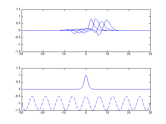
Refer to caption
Figure 1. Upper: Evolution of the free surface for different times t=2.5,5,7.5 and 10. Lower: bottom topography and initial condition.
Refer to caption
Figure 2. Upper: Evolution of the free surface for different times t=2.5,5,7,5 and 10 . Lower: bottom topography and initial condition.

Figures 3 displays the convergence curve for this example. We plot the logarithm of the error (in norm H1×L2superscript𝐻1superscript𝐿2H^{1}\times L^{2}) in function of the logarithm of the time step Δt.Δ𝑡\Delta t. The convergence numerical order is then given by the slope of this curve. For reference, a small line (the dashed line) of slope one is added in this figure. We see that the numerical rate of convergence is greater than 1.

Refer to caption
Figure 3. Convergence curve (for the H1×L2superscript𝐻1superscript𝐿2H^{1}\times L^{2}-norm) for the Lie method for two bottoms : bump (black line) and ripple bottom (blue line) for T=10.𝑇10T=10.

5.2. Example 2: Non smooth topographies

In this example we study the evolution of water waves over a rough bottom. This problem is still a mathematical issue. Many models derived from the Euler equations suppose that the bathymetry is smooth. Even worse, a non smooth bathymetry introduces singular terms in these models. This issue is particularly easy to see for shallow waters models. To handle this, Hamilton ([20]) and Nachbin ([30]) used a coformal mapping to derive long waves models. Notice also the work of Cathala ([10]) who derived alternatives Saint-Venant equations and Boussinesq systems with non smooth topographies which do not involve any singular terms. We notice that the Saut-Xu equations (1.1) can handle a non smooth topography (see Theorem (2.2)) and our numerical scheme too (see Theorem (4.6)).

In the following, we give an example with a non smooth bathymetry. We consider the following initial conditions and bathymetry

ζ0(x)=v0(x)=ex2 and b(x)=β4(1+tanh(100(x2)))(1tanh(100(x8))).subscript𝜁0𝑥subscript𝑣0𝑥superscript𝑒superscript𝑥2 and 𝑏𝑥𝛽41100𝑥21100𝑥8\zeta_{0}(x)=v_{0}(x)=e^{-x^{2}}\text{ and }b(x)=\frac{\beta}{4}(1+\tanh(100(x-2)))(1-\tanh(100(x-8))).

We decided to take μ=1𝜇1\mu=1, β=0.5𝛽0.5\beta=0.5, ε=0.1𝜀0.1\varepsilon=0.1, N=28,Δx=2L/Nformulae-sequence𝑁superscript28Δ𝑥2𝐿𝑁N=2^{8},\Delta x=2L/N where N is the mesh modes number, L=20𝐿20L=20 the length of the domain. The time step ΔtΔ𝑡\Delta t is chosen iteratively in a way that the CFL condition (5.3) is satisfied. Figure 4 displays the evolution of the surface ζ𝜁\zeta for different times over the bottom.
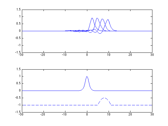
Refer to caption
Figure 4. Evolution of the free surface (blue lines) for different times t=0,3,6,9 and 12 over a rough bottom (black line).

5.3. Example 3: Boussinesq regime

In Section 3, we crucially use the fact that μ𝜇\mu is bounded from below. In this example, we test our scheme for small values of μ𝜇\mu (also called the shallow water regime). We show that our scheme is still valid even if we do not have a proof of the convergence of our scheme in this regime. In the shallow water regime, there is a huge literature for asymptotic models (see for instance [24]). Among all these asymptotic models, we have the KdV equation. It is a model obtained under the Boussinesq regime, i.e. when ε=μ𝜀𝜇\varepsilon=\mu, β=0𝛽0\beta=0 and μ𝜇\mu small. In the following, we formally derive a KdV equation from the Saut-Xu equations and we give numerical simulations in this setting.

We recall that, without the assumption ν=1μ𝜈1𝜇\nu=\frac{1}{\mu}, the Saut-Xu equations are given by the system (2.3). Notice also that

(5.4) μ=μx13μ32x3+𝒪(μ2).subscript𝜇𝜇subscript𝑥13superscript𝜇32superscriptsubscript𝑥3𝒪superscript𝜇2\mathcal{H}_{\mu}=-\sqrt{\mu}\partial_{x}-\frac{1}{3}\mu^{\frac{3}{2}}\partial_{x}^{3}+\mathcal{O}(\mu^{2}).

Then if we assume that μ=ε𝜇𝜀\mu=\varepsilon, ν=1𝜈1\nu=1 (since ν1similar-to𝜈1\nu\sim 1 if μ𝜇\mu is small) and we drop all the terms of order 𝒪(μ2)𝒪superscript𝜇2\mathcal{O}(\mu^{2}) in System (2.3), we obtain the following equations

(5.5) {tζ+xv+μvxζ12μ32vxζ+13μx3v+μζxv=0,tv+xζ+μvxv+μ3212vxv=0.\left\{\begin{aligned} &\partial_{t}\zeta+\partial_{x}v+\mu v\partial_{x}\zeta-\frac{1}{2}\mu^{\frac{3}{2}}v\partial_{x}\zeta+\frac{1}{3}\mu\partial_{x}^{3}v+\mu\zeta\partial_{x}v=0,\\ &\partial_{t}v+\partial_{x}\zeta+\mu v\partial_{x}v+\mu^{\frac{3}{2}}\frac{1}{2}v\partial_{x}v=0.\end{aligned}\right.

Formally, the solutions of this system are close to the solutions of (2.3) with an accuracy of order 𝒪(μ2)𝒪superscript𝜇2\mathcal{O}(\mu^{2}). Notice that this system is not a standard Boussinesq system (in the sense of [4] or [24]) because of our nonlinear change of variables (2.2). Using the approach developed in [35], [5], [2] (see also Part 7.1.1 in [24]) we can check that, formally, the following KdV equation is an asymptotic model of the system (5.5)

(5.6) tf+32fxf+16x3f=0.subscript𝑡𝑓32𝑓subscript𝑥𝑓16superscriptsubscript𝑥3𝑓0\partial_{t}f+\frac{3}{2}f\partial_{x}f+\frac{1}{6}\partial_{x}^{3}f=0.

This means that if we solve (5.5) with the initial data (f0,f0)subscript𝑓0subscript𝑓0\left(f_{0},f_{0}\right) and (5.6) with the initial datum f0subscript𝑓0f_{0}, the solution (ζ,v)(t,x)𝜁𝑣𝑡𝑥\left(\zeta,v\right)(t,x) of (5.5) is close to (f,f)(μt,xt)𝑓𝑓𝜇𝑡𝑥𝑡\left(f,f\right)(\mu t,x-t). Furthermore, if we take f0(x)=αsech2(34αx)subscript𝑓0𝑥𝛼superscriptsech234𝛼𝑥f_{0}(x)=\alpha\text{sech}^{2}\left(\sqrt{\frac{3}{4}\alpha}x\right), the solution f𝑓f of the KdV equation with this initial datum is the soliton f(t,x)=f0(xct)𝑓𝑡𝑥subscript𝑓0𝑥𝑐𝑡f(t,x)=f_{0}(x-ct) with c=α2𝑐𝛼2c=\frac{\alpha}{2}. Hence, in this case, the solution of (5.5) and (2.3) are close to a soliton.

In the following we check that the solution to (1.1) is indeed close to the KdV solution when μ𝜇\mu is small. We simulate one soliton. We took v0(x)=ζ0(x)=sech2(32x)subscript𝑣0𝑥subscript𝜁0𝑥superscriptsech232𝑥v_{0}(x)=\zeta_{0}(x)=\operatorname{sech}^{2}\left(\frac{\sqrt{3}}{2}x\right) , ε=μ=0.01𝜀𝜇0.01\varepsilon=\mu=0.01, α=1𝛼1\alpha=1 and the final time is T=10𝑇10T=10. We decided to take N=29,Δx=2L/Nformulae-sequence𝑁superscript29Δ𝑥2𝐿𝑁N=2^{9},\Delta x=2L/N where N is the mesh modes number, L=30𝐿30L=30 the length of the domain. The time step ΔtΔ𝑡\Delta t is chosen iteratively in a way that the CFL condition (5.3) is satisfied. Figure 5 represents the evolution of this soliton at different times. Hence, our sheme is still valid when μ𝜇\mu is small.

In deep water (μ𝜇\mu not small), the KdV approximation ceases to be a good approximation. In order to get some insight on the range of validity of the KdV approximation, we compare in Figure 6 the solution of (1.1) to the exact soliton after a time T=10𝑇10T=10 for various values of μ𝜇\mu. We took the same numerical parameters that before. We notice that even for ε=μ=0.1𝜀𝜇0.1\varepsilon=\mu=0.1 and a final time T=1μ𝑇1𝜇T=\frac{1}{\mu}, the KdV approximation remains a good approximation of the Saut-Xu system.
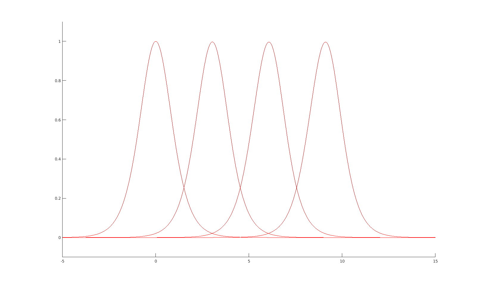
Refer to caption
Figure 5. Evolution of the soliton at different times t=0,3,6,9𝑡0369t=0,3,6,9 (ε=0.01𝜀0.01\varepsilon=0.01).
Refer to caption
Figure 6. Difference after a time T=10𝑇10T=10 between a real soliton and a soliton generated by our scheme with the same initial data and for different values of ε=μ𝜀𝜇\varepsilon=\mu. Abscissa : value of ε𝜀\varepsilon; Ordinate : quotient of the difference after a final time T=10𝑇10T=10 by the maximum of the soliton.

5.4. Example 4: Rapidly varying topographies

In this example we study the evolution of water waves over a rapidly varying periodic bottom. We assume that μ=1𝜇1\mu=1. This problem is linked to the Bragg reflection phenomenon (see for instance [29], [25], [19]). We take

(5.7) ζ0=v0=sech2(32x) and b(x)=cos(αx).subscript𝜁0subscript𝑣0superscriptsech232𝑥 and 𝑏𝑥𝛼𝑥\zeta_{0}=v_{0}=\text{sech}^{2}\left(\frac{\sqrt{3}}{2}x\right)\text{ and }b(x)=\cos(\alpha x).

We decided to take N=29,Δx=2L/Nformulae-sequence𝑁superscript29Δ𝑥2𝐿𝑁N=2^{9},\Delta x=2L/N where N is the mesh modes number, L=30𝐿30L=30 the length of the domain. The time step ΔtΔ𝑡\Delta t is chosen iteratively in a way that the CFL condition (5.3) is satisfied. Figure 7 compares the evolution of water waves when we take α=10𝛼10\alpha=10 (blue line) and when we take b(x)=0𝑏𝑥0b(x)=0 (blue line). Figure 8 displays the difference between the case of a flat bottom and the case of a bottom of the form b(x)=cos(αx)𝑏𝑥𝛼𝑥b(x)=\cos(\alpha x) for different values of α𝛼\alpha. We observe an homogenization effect when α𝛼\alpha is large. It seems that when α𝛼\alpha goes to infinity, a solution of the Saut-Xu equations converges to a solution of the Saut-Xu equations with a flat bottom (corresponding to the mean of b𝑏b). Notice that this result is different from what we could see in the literature ( for instance [13] or [15]), since we take a bottom of the form b(x)=cos(αx)𝑏𝑥𝛼𝑥b(x)=\cos(\alpha x) and not of the form b(x)=1αcos(αx)𝑏𝑥1𝛼𝛼𝑥b(x)=\frac{1}{\alpha}\cos(\alpha x). Our numerical simulations suggest therefore a homogenization effect for large amplitude bottom variations that has not been investigated so far.
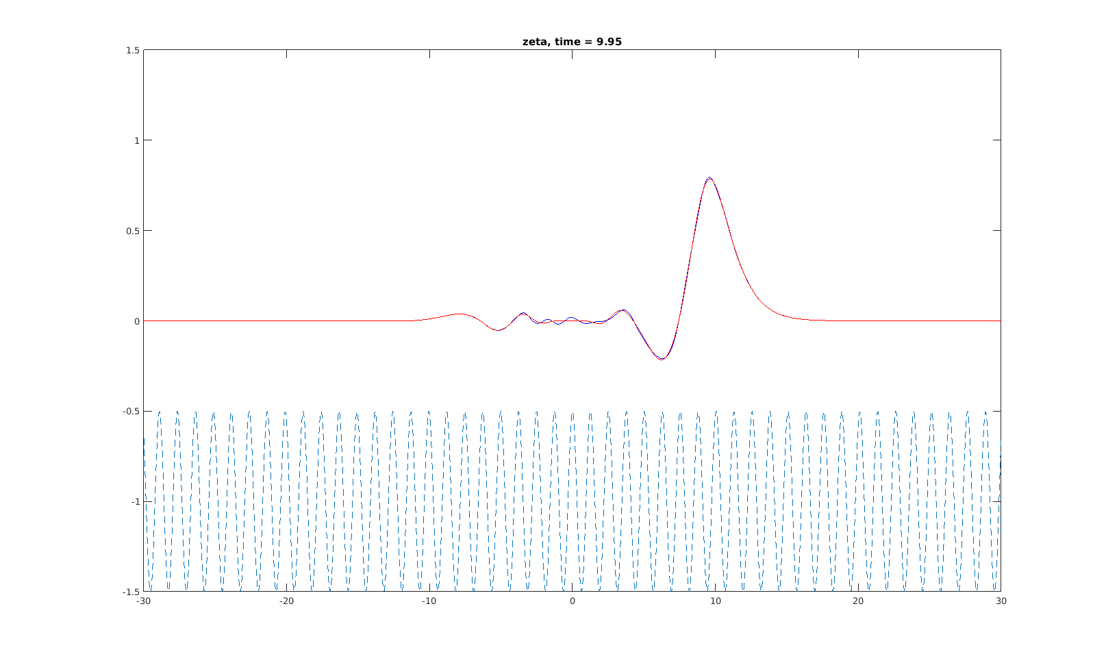
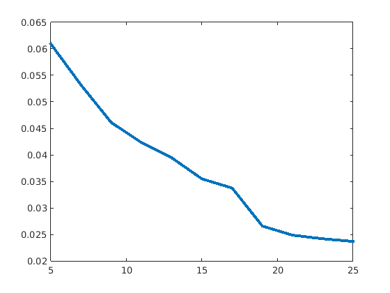
Refer to caption
Figure 7. Comparison between the evolution of a water wave (blue line) over a bottom of the form b(x)=cos(10x)𝑏𝑥10𝑥b(x)=\cos(10x) (dashed line) and the evolution of a water wave over a flat bottom (black line). ε=0.05𝜀0.05\varepsilon=0.05, β=0.5𝛽0.5\beta=0.5.
Refer to caption
Figure 8. Difference between a water wave over a rapidly varying topography b(x)=cos(αx)𝑏𝑥𝛼𝑥b(x)=\cos(\alpha x) and a water wave over a flat bottom. Abscissa : value of α𝛼\alpha; Ordinate : quotient of the difference after a final time T=10𝑇10T=10 by the maximum of ζ0subscript𝜁0\zeta_{0}.

Appendix A

In this part, we give some estimate for the operator μsubscript𝜇\mathcal{H}_{\mu} and some standard product and commutator estimates. For the estimates for μsubscript𝜇\mathcal{H}_{\mu}, we refer to part III in [34]. For the other estimates we refer to [1] and [23]. We recall that μsubscript𝜇\mathcal{H}_{\mu} is defined by

μ=tanh(μD)Dx.subscript𝜇𝜇𝐷𝐷subscript𝑥\mathcal{H}_{\mu}=-\frac{\tanh(\sqrt{\mu}D)}{D}\partial_{x}.

First, we show that μsubscript𝜇\mathcal{H}_{\mu} is a zero-order operator.

Proposition A.1.

Let s0𝑠0s\geq 0 and μ𝜇\mu satisfying Condition (1.3). Then,

|μu|HsC(μmax)|u|Hs.subscriptsubscript𝜇𝑢superscript𝐻𝑠𝐶subscript𝜇subscript𝑢superscript𝐻𝑠\left\lvert\mathcal{H}_{\mu}u\right\rvert_{H^{s}}\leq C\left(\mu_{\max}\right)\left\lvert u\right\rvert_{H^{s}}.

Furthermore, for all sr0𝑠𝑟0s\geq r\geq 0,

|(μ2+1)u|HsCr(1μmin)|u|Hr.subscriptsuperscriptsubscript𝜇21𝑢superscript𝐻𝑠subscript𝐶𝑟1subscript𝜇subscript𝑢superscript𝐻𝑟\left\lvert\left(\mathcal{H}_{\mu}^{2}+1\right)u\right\rvert_{H^{s}}\leq C_{r}\left(\frac{1}{\mu_{\min}}\right)\left\lvert u\right\rvert_{H^{r}}.

Then, we give a commutator estimate for μsubscript𝜇\mathcal{H}_{\mu}.

Proposition A.2.

Let s0𝑠0s\geq 0, t0>12subscript𝑡012t_{0}>\frac{1}{2}, r0𝑟0r\geq 0, and μ𝜇\mu satisfying Condition (1.3). Then,

|[μ,a]u|2C|a|Ht0|f|2,subscriptsubscript𝜇𝑎𝑢2𝐶subscript𝑎superscript𝐻subscript𝑡0subscript𝑓2\left\lvert\left[\mathcal{H}_{\mu},a\right]u\right\rvert_{2}\leq C\left\lvert a\right\rvert_{H^{t_{0}}}\left\lvert f\right\rvert_{2},
||ξ|s[μ,a]u^|2C(1μmin)|a|Hr+s|(1+|ξ|)t0|ξ|ru^|2,subscriptsuperscript𝜉𝑠^subscript𝜇𝑎𝑢2𝐶1subscript𝜇subscript𝑎superscript𝐻𝑟𝑠subscriptsuperscript1𝜉subscript𝑡0superscript𝜉𝑟^𝑢2\left\lvert|\xi|^{s}\widehat{\left[\mathcal{H}_{\mu},a\right]u}\right\rvert_{2}\leq C\left(\frac{1}{\mu_{\min}}\right)\left\lvert a\right\rvert_{H^{r+s}}\left\lvert\frac{\left(1+|\xi|\right)^{t_{0}}}{|\xi|^{r}}\widehat{u}\right\rvert_{2},

and

||ξ|s[μ,a]u^|2C(1μmin)|a|Hr+s+t0|1|ξ|ru^|2.subscriptsuperscript𝜉𝑠^subscript𝜇𝑎𝑢2𝐶1subscript𝜇subscript𝑎superscript𝐻𝑟𝑠subscript𝑡0subscript1superscript𝜉𝑟^𝑢2\left\lvert|\xi|^{s}\widehat{\left[\mathcal{H}_{\mu},a\right]u}\right\rvert_{2}\leq C\left(\frac{1}{\mu_{\min}}\right)\left\lvert a\right\rvert_{H^{r+s+t_{0}}}\left\lvert\frac{1}{|\xi|^{r}}\widehat{u}\right\rvert_{2}.

We recall the well-known Coifman-Meyer estimate. We recall also that ΛΛ\Lambda is the Fourier multiplier Λ=1+D2Λ1superscript𝐷2\Lambda=\sqrt{1+D^{2}}.

Proposition A.3.

Let s>32𝑠32s>\frac{3}{2}, uHs()𝑢superscript𝐻𝑠u\in H^{s}(\mathbb{R}) and vHs1()𝑣superscript𝐻𝑠1v\in H^{s-1}(\mathbb{R}). Then we have the following commutator estimate

|[Λs,u]v|2C|u|Hs|v|Hs1.subscriptsuperscriptΛ𝑠𝑢𝑣2𝐶subscript𝑢superscript𝐻𝑠subscript𝑣superscript𝐻𝑠1\left\lvert\left[\Lambda^{s},u\right]v\right\rvert_{2}\leq C\left\lvert u\right\rvert_{H^{s}}\left\lvert v\right\rvert_{H^{s-1}}.

We recall also the following product estimate.

Proposition A.4.

Let s1,s2,ssubscript𝑠1subscript𝑠2𝑠s_{1},s_{2},s such that s1+s20subscript𝑠1subscript𝑠20s_{1}+s_{2}\geq 0, smin(s1,s2)𝑠subscript𝑠1subscript𝑠2s\leq\min\left(s_{1},s_{2}\right) and s<s1+s212𝑠subscript𝑠1subscript𝑠212s<s_{1}+s_{2}-\frac{1}{2}. Let uHs1()𝑢superscript𝐻subscript𝑠1u\in H^{s_{1}}(\mathbb{R}) and vHs2()𝑣superscript𝐻subscript𝑠2v\in H^{s_{2}}(\mathbb{R}). Then,

|uv|HsC|u|Hs1|v|Hs2.subscript𝑢𝑣superscript𝐻𝑠𝐶subscript𝑢superscript𝐻subscript𝑠1subscript𝑣superscript𝐻subscript𝑠2\left\lvert uv\right\rvert_{H^{s}}\leq C\left\lvert u\right\rvert_{H^{s_{1}}}\left\lvert v\right\rvert_{H^{s_{2}}}.

Acknowledgments

The second author has been partially funded by the ANR project Dyficolti ANR-13-BS01-0003.

References

  • [1] S. Alinhac and P. Gérard. Opérateurs pseudo-différentiels et théorème de Nash-Moser. Savoirs Actuels. [Current Scholarship]. InterEditions, Paris; Éditions du Centre National de la Recherche Scientifique (CNRS), Meudon, 1991.
  • [2] B. Alvarez-Samaniego and D. Lannes. Large time existence for 3D water-waves and asymptotics. Invent. Math., 171(3):485–541, 2008.
  • [3] D. M. Ambrose, J. L. Bona, and D. P. Nicholls. On ill-posedness of truncated series models for water waves. Proc. R. Soc. Lond. Ser. A Math. Phys. Eng. Sci., 470(2166):20130849, 16, 2014.
  • [4] J. L. Bona, M. Chen, and J.-C. Saut. Boussinesq equations and other systems for small-amplitude long waves in nonlinear dispersive media. I. Derivation and linear theory. J. Nonlinear Sci., 12(4):283–318, 2002.
  • [5] J. L. Bona, T. Colin, and D. Lannes. Long wave approximations for water waves. Arch. Ration. Mech. Anal., 178(3):373–410, 2005.
  • [6] P. Bonneton, E. Barthelemy, F. Chazel, R. Cienfuegos, D. Lannes, F. Marche, and M. Tissier. Recent advances in serre-green naghdi modelling for wave transformation, breaking and runup processes. European Journal of Mechanics - B Fluids, 30(6):589 – 597, 2011. Special Issue: Nearshore Hydrodynamics.
  • [7] P. Bonneton, F. Chazel, D. Lannes, F. Marche, and M. Tissier. A splitting approach for the fully nonlinear and weakly dispersive green-naghdi model. Journal of Computational Physics, 230(4):1479 – 1498, 2011.
  • [8] P. Bonneton and D. Lannes. Derivation of asymptotic two-dimensional time-dependent equations for surface water wave propagation. Phys. Fluids, 21, 2009.
  • [9] R. Carles. On Fourier time-splitting methods for nonlinear Schrödinger equations in the semiclassical limit. SIAM J. Numer. Anal., 51(6):3232–3258, 2013.
  • [10] M. Cathala. Asymptotic shallow water models with non smooth topographies. Monatshefte für Mathematik, pages 1–29, 2014.
  • [11] P. Chartier, L. Le treust, and F. Méhats. Uniformly accurate time-splitting methods for the semiclassical schrödinger equation part 2 : numerical analysis of the linear case. arXiv : 1601.04825v1, 2016.
  • [12] W. Choi. Nonlinear evolution equations for two-dimensional surface waves in a fluid of finite depth. J. Fluid Mech., 295:381–394, 1995.
  • [13] L. Chupin. Roughness effect on Neumann boundary condition. Asymptot. Anal., 78(1-2):85–121, 2012.
  • [14] W. Craig, P. Guyenne, D. P. Nicholls, and C. Sulem. Hamiltonian long-wave expansions for water waves over a rough bottom. Proc. R. Soc. Lond. Ser. A Math. Phys. Eng. Sci., 461:839–873, 2005.
  • [15] W. Craig, D. Lannes, and C. Sulem. Water waves over a rough bottom in the shallow water regime. Ann. Inst. H. Poincaré Anal. Non Linéaire, 29(2):233–259, 2012.
  • [16] W. Craig and C. Sulem. Numerical simulation of gravity waves. J. Comput. Phys., 108(1):73–83, 1993.
  • [17] W. Craig, C. Sulem, and P.-L. Sulem. Nonlinear modulation of gravity waves: a rigorous approach. Nonlinearity, 5(2):497–522, 1992.
  • [18] P. Guyenne and D. P. Nicholls. Numerical simulation of solitary waves on plane slopes. Math. Comput. Simul., 69:269–281, 2005.
  • [19] P. Guyenne and D. P. Nicholls. A high-order spectral method for nonlinear water waves over moving bottom topography. SIAM J. Sci. Computer, no. 1:81–101, 2007-08.
  • [20] James Hamilton. Differential equations for long-period gravity waves on fluid of rapidly varying depth. J. Fluid Mech., 83(2):289–310, 1977.
  • [21] H. Holden, C. Lubich, and N. H. Risebro. Operator splitting for partial differential equations with Burgers nonlinearity. Math. Comput., 82(281), 2013.
  • [22] T. Iguchi. A shallow water approximation for water waves. J. Math. Kyoto Univ., 49(1):13–55, 2009.
  • [23] D. Lannes. Sharp estimates for pseudo-differential operators with symbols of limited smoothness and commutators. J. Funct. Anal., 232(2):495–539, 2006.
  • [24] D. Lannes. The water waves problem, volume 188 of Mathematical Surveys and Monographs. American Mathematical Society, Providence, RI, 2013. Mathematical analysis and asymptotics.
  • [25] Y. Liu and D.K.P. Yue. On generalized Bragg scattering of surface waves by bottom ripples. Journal of Fluid Mechanics, 356:297–326, 1998.
  • [26] C. Lubich. On splitting methods for Schrödinger-Poisson and cubic nonlinear Schrödinger equations. Math. Comp., 77(264):2141–2153, 2008.
  • [27] Y. Matsuno. Nonlinear evolutions of surface gravity waves on fluid of finite depth. Phys. Rev. Lett., 69(4):609–611, 1992.
  • [28] Y. Matsuno. Nonlinear evolution of surface gravity waves over an uneven bottom. J. Fluid Mech., 249:121–133, 1993.
  • [29] C. C. Mei. Resonant reflection of surface water waves by periodic sandbars. Journal of Fluid Mechanics, 152:315–335, 3 1985.
  • [30] André Nachbin. A terrain-following Boussinesq system. SIAM J. Appl. Math., 63(3):905–922, 2003.
  • [31] D. P. Nicholls and F. Reitich. Stability of high–order perturbative methods for the computation of Dirichlet–Neumann operators. Journal of Computational Physics, 170(1):276–298, 2001.
  • [32] D. L. Ropp and J. N. Shadid. Stability of operator splitting methods for systems with indefinite operators: advection-diffusion-reaction systems. J. Comput. Phys., 228(9):3508–3516, 2009.
  • [33] A. Sacchetti. Spectral splitting method for nonlinear Schrödinger equations with singular potential. J. Comput. Phys., 227(2):1483–1499, 2007.
  • [34] J. C. Saut and L. Xu. Well-posedness on large time for a modified full dispersion system of surface waves. J. Math. Phys., 53(11):115606, 23, 2012.
  • [35] G. Schneider and C. E. Wayne. Corrigendum: The long-wave limit for the water wave problem I. The case of zero surface tension [mr1780702]. Comm. Pure Appl. Math., 65(5):587–591, 2012.
  • [36] R. A. Smith. An operator expansion formalism for nonlinear surface waves over variable depth. J. Fluid Mech., 363:333–347, 1998.
  • [37] T. R. Taha and M. J. Ablowitz. Analytical and numerical aspects of certain nonlinear evolution equations. II. Numerical, nonlinear Schrödinger equation. J. Comput. Phys., 55(2):203–230, 1984.
  • [38] V.E Zakharov. Stability of periodic waves of finite amplitude on the surface of a deep fluid. J. Applied Mech. Tech. Phys., 9:190–194, 1968.