Position-Indexed Formulations for Kidney Exchange
Abstract
A kidney exchange is an organized barter market where patients in need of a kidney swap willing but incompatible donors. Determining an optimal set of exchanges is theoretically and empirically hard. Traditionally, exchanges took place in cycles, with each participating patient-donor pair both giving and receiving a kidney. The recent introduction of chains, where a donor without a paired patient triggers a sequence of donations without requiring a kidney in return, increased the efficacy of fielded kidney exchanges—while also dramatically raising the empirical computational hardness of clearing the market in practice. While chains can be quite long, unbounded-length chains are not desirable: planned donations can fail before transplant for a variety of reasons, and the failure of a single donation causes the rest of that chain to fail, so parallel shorter chains are better in practice.
In this paper, we address the tractable clearing of kidney exchanges with short cycles and chains that are long but bounded. This corresponds to the practice at most modern fielded kidney exchanges. We introduce three new integer programming formulations, two of which are compact. Furthermore, one of these models has a linear programming relaxation that is exactly as tight as the previous tightest formulation (which was not compact) for instances in which each donor has a paired patient. On real data from the UNOS nationwide exchange in the United States and the NLDKSS nationwide exchange in the United Kingdom, as well as on generated realistic large-scale data, we show that our new models are competitive with all existing solvers—in many cases outperforming all other solvers by orders of magnitude.
Finally, we note that our position-indexed chain-edge formulation can be modified in a straightforward way to take post-match edge failure into account, under the restriction that edges have equal probabilities of failure. Post-match edge failure is a primary source of inefficiency in presently-fielded kidney exchanges. We show how to implement such failure-aware matching in our model, and also extend the state-of-the-art general branch-and-price-based non-compact formulation for the failure-aware problem to run its pricing problem in polynomial time.
doi:
2940716.2940759keywords:
Kidney exchange; matching markets; stochastic matching; integer programming; branch and priceJohn P. Dickerson, David F. Manlove, Benjamin Plaut, Tuomas Sandholm, and James Trimble, 2016. Position-Indexed Formulations for Kidney Exchange.
Work supported by NSF grants IIS-1320620 and IIS-1546752, ARO grant W911NF-16-1-0061, Facebook and Siebel fellowships, and by XSEDE through the Pittsburgh Supercomputing Center (Dickerson / Plaut / Sandholm), and by EPSRC grants EP/K010042/1, EP/K503903/1 and EP/N508792/1 (Manlove / Trimble).
Authors’ addresses: J.P. Dickerson, B. Plaut, and T. Sandholm, Computer Science Department, Carnegie Mellon University; email: {dickerson,sandholm}@cs.cmu.edu, bplaut@stanford.edu; D.F. Manlove and J. Trimble, School of Computing Science, University of Glasgow; email: david.manlove@glasgow.ac.uk, james.trimble@yahoo.co.uk.
1 Introduction
Transplantation is the most effective treatment for kidney failure, yet transplant waiting lists have grown rapidly in many countries. In the United States alone, the kidney transplant waiting list grew from people in to people in [Hart et al. (2016)]. In order to increase the supply of kidneys for transplant, kidney exchange schemes now operate in several countries, including the United States, United Kingdom, Netherlands, and South Korea.
A kidney exchange [Rapaport (1986), Roth et al. (2004)] is a centrally-administered barter exchange market for kidneys. If a patient with end-stage renal disease has a friend or family member who is willing to donate a kidney to him, but unable to do so due to blood- or tissue-type incompatibility, the patient may enter the exchange in the hope of exchanging his donor with the donor of another participating patient. Three-way exchanges are also possible, but most schemes do not carry out four-way or longer exchanges due to the requirement that transplants be carried out simultaneously, and the risk that one of the participants may need to withdraw, in which case the cycle does not go to execution and the pairs go back into the kidney exchange pool.
The scheme administrator carries out periodic “match runs” in which exchanges are selected in order to maximize the number of planned transplants, or a similar goal—perhaps prioritizing pediatric patients, or to those who have been waiting the longest.
A more recent development has been the introduction of non-directed donors (NDDs) to kidney exchange schemes [Montgomery et al. (2006), Roth et al. (2006)]. An NDD enters the scheme with the intention of donating a kidney, but without a paired recipient. Such a donor initiates a chain, in which the paired donor of each patient who receives a kidney donates a kidney to the next patient. In contrast to cyclic exchanges, chains can be carried out non-simultaneously, since patients later in the chain are not waiting to be “repaid” for a donation that has already been made. In practice, it is desirable to impose a cap on chain length, since there is an increasing chance that the final exchanges planned for a chain will not proceed as the chain length is increased (due to various reasons such as pre-transplant crossmatch incompatibility, death of a recipient before transplant, the recipient receiving a deceased-donor kidney, and so on).
In many fielded kidney exchanges, an optimal solution is found by using an integer programming (IP) solver to find a set of disjoint cyclic exchanges and chains that maximizes some scoring function. This approach has been tractable so far; \citeNManlove15:Paired report that each instance up to October in the United Kingdom’s National Living Donor Kidney Sharing Schemes (NLDKSS)—one of the largest kidney exchange schemes—could be solved in under a second, with similar results using state-of-the-art solvers at other large exchanges in the US [Anderson et al. (2015), Plaut et al. (2016a)] and the Netherlands [Glorie et al. (2014)]. However, there is an urgent need for faster kidney exchange algorithms, for three reasons:
-
•
Schemes have recently increased chain-length caps, and we expect further increases as more schemes evolve towards using nonsimultaneous extended altruistic donor (NEAD) chains [Rees et al. (2009)], which can extend across dozens of transplants.
-
•
Opportunities exist for cross-border schemes, which will greatly increase the size of the problem to be solved; indeed, collaborations have already occurred between, for example, the USA and Greece, and between Portugal and Spain.
-
•
The run time for kidney exchange algorithms depends on the problem instance, and is difficult to predict. It is desirable to have improved algorithms to insure against the possibility that future instances will be intractable for current solvers.
With that motivation, this paper presents new scalable integer-programming-based approaches to optimally clearing large kidney exchange schemes, including two models which can comfortably handle chain caps greater than .
1.1 Prior research
Substantial prior research helped grow kidney exchange from a thought experiment to its present increasingly-ubiquitous state. We briefly overview the literature from economics, computer science, and operations research.
Theoretical basis for kidney exchange
Roth et al. 2004; 2005; 2007 set the groundwork for large-scale organized kidney exchange. These papers explored what efficient matchings in a steady-state kidney exchange would look like; extensions by Ashlagi et al. (2012), Ashlagi and Roth (2014), and Ding et al. (2015) address shortcomings in those theoretical models that appeared as kidney exchange became reality. Game-theoretic models of kidney exchange, where transplant centers are viewed as agents with a private type consisting of their internal pools, were presented and explored by Ashlagi and Roth (2014), Toulis and Parkes (2015), and Ashlagi et al. (2015). Various forms of dynamism, like uncertainty over the possible future vertices in the pool Ünver (2010); Ashlagi et al. (2013); Akbarpour et al. (2014) or uncertainty over the existence of particular edges Blum et al. (2013); Dickerson et al. (2013); Blum et al. (2015) have been explored from both an economic and algorithmic efficiency point of view.
Practical approaches to the kidney exchange clearing problem
The two fundamental IP models for kidney exchange are the cycle formulation, which includes one binary decision variable for each feasible cycle or chain, and the edge formulation, which includes one decision variable for each compatible pair of agents Abraham et al. (2007); Roth et al. (2007). In the cycle formulation, the number of constraints is sublinear in the input size, but the number of variables is exponential. In the edge formulation, the number of variables is linear but the number of constraints is exponential. Optimally solving these models has been an ongoing challenge for the past decade.
Constantino et al. (2013) introduced the first two compact IP formulations for kidney exchange, where compact means that the counts of variables and constraints are polynomial in the size of the input. Their extended edge formulation was shown empirically to be effective in finding the optimal solution where the cycle-length cap is greater than , particularly on dense graphs. However, each of the compact formulations introduced by Constantino et al. has a weaker linear program (LP) relaxation than the cycle formulation, even in the absence of NDDs.
The EE-MTZ model Mak-Hau (2015), another compact formulation, uses the variables and constraints of the extended edge formulation to model cycles and a variant of the Miller-Tucker-Zemlin model for the traveling salesman problem to model chains. The same paper introduces the exponentially-sized SPLIT-MTZ model, which adds redundant constraints to the edge formulation in order to tighten the LP relaxation.
A number of kidney exchange algorithms use the cycle formulation with branch and price Barnhart et al. (1998) to avoid the need to hold an exponential number of variables in memory Abraham et al. (2007); Dickerson et al. (2013); Glorie et al. (2014); Klimentova et al. (2014); Plaut et al. (2016a). These have been the fastest algorithms to date for the kidney exchange problem.
An alternative approach to avoiding the cost of keeping the entire model in memory has been constraint generation, using variants of the edge formulation Abraham et al. (2007). Anderson et al. (2015) describe an approach based on an algorithm for the prize-collecting traveling salesman problem. This algorithm is particularly effective for solving instances where the cycle-length cap is and there is no cap on the length of chains, but it is outperformed by branch-and-price-based approaches if a finite chain-length cap is used Plaut et al. (2016a).
Alternative objectives for the kidney exchange problem include maximizing the expected number of transplants subject to post-match arc and vertex failures Dickerson et al. (2013); Pedroso (2014); Alvelos et al. (2015). Some fielded exchanges use lexicographic optimisation of a hierarchy of objectives Glorie et al. (2014); Manlove and O’Malley (2015); we note that our models can be augmented to support this class of objective function.
1.2 Our contribution
This paper introduces three integer program formulations for the kidney exchange problem, two of which are compact. Model size (i.e., memory footprint) often constrains today’s kidney exchange solvers; critically, our models are typically much smaller than the state of the art while managing to maintain tight linear program relaxations (LPRs)—which in practice is quite important to proving optimality quickly.
In Section 3, we introduce the position-indexed edge formulation (PIEF), a model for the kidney exchange problem with only cycles that is substantially smaller than, yet has an LPR equivalent to, the model with the tightest LPR for the cycles-only version of the problem Abraham et al. (2007); Roth et al. (2007). Section 3 presents the position-indexed chain-edge formulation (PICEF) which compactly brings chains into the model via a polynomial number of decision variables; the number of cycle decision variables is exponential in just the maximum cycle length (which is typically only or in fielded exchanges). To address that latter exponential reliance on the cycle length, we also present a branch-and-price-based implementation of PICEF. Finally, in Appendix 10 we present the hybrid position-indexed edge formulation (HPIEF), which combines PIEF and PICEF to yield a compact formulation.
Throughout, we prove new results regarding the tightness of the LPRs of our models relative to the current state of the art. The tightness of these relaxations hints that our formulations will be competitive in practice; toward that end, we provide extensive experimental evidence that they are. In particular, we show that at least one of PICEF and HPIEF is faster than the best solver from all those provably-optimal solvers contributed in earlier papers that we evaluated in % of instances considered, with the speed-ups being most evident for larger instance sizes and larger chain caps. In Section 6, we use real and generated data from two nationwide kidney exchange programs—one in the UK, and one in the US—to compare our formulations against other competitive solvers Abraham et al. (2007); Klimentova et al. (2014); Anderson et al. (2015); Plaut et al. (2016a). Our new formulations are on par or faster than all other solvers, outperforming all other solvers by orders of magnitude on many problem instances.
Finally, we demonstrate that our PICEF formulation can be adapted straightforwardly to the so-called failure-aware model where arcs probabilistically fail after algorithmic match but before transplantation, and we show how to adapt a recent (non-compact) branch-and-price-based formulation due to Dickerson et al. (2013) to perform pricing in polynomial time (Section 6).
2 Preliminaries
Given a pool consisting of patient-donor pairs and non-directed donors (NDDs), we model the kidney exchange problem using a directed graph . The set of vertices is partitioned into representing the NDDs and representing the patient-donor pairs.
For each and each , contains the arc if and only if NDD is compatible with patient . For each and each , contains the arc if and only if the paired donor111In this paper, we assume that each patient has a single paired donor. In practice, a patient may have multiple donors; this can be modeled by regarding such a patient ’s vertex in as representing and all of her paired donors; an arc in then represents compatibility between at least one of ’s donors and patient . Our model can also handle patients with no paired donor by drawing a vertex with no out edges. of patient is compatible with patient . Each arc has a weight representing the priority that the scheme administrator gives to that transplant. If the objective is to maximize the number of transplants, each arc has unit weight; most fielded exchanges use weights to encode various prioritization schemes and other value judgments about potential transplants.
Since NDDs do not have paired patients, each vertex representing an NDD has no incoming arcs. Moreover, we assume that no patient is compatible with her own paired donor, and therefore that the digraph has no loops. (The IP models introduced in this paper can trivially be adapted to the case where loops exist by adding a binary variable for each loop and modifying the objective and capacity constraints accordingly.)
We use the term chain to refer to a path in the digraph initiated by an NDD vertex, and cycle to refer to a cycle in the directed graph (which must involve only vertices in , since vertices in have no incoming arcs). The weight of each cycle or chain is defined as the sum of its arc weights.
Given a maximum cycle size and a maximum chain length , the kidney exchange problem is an optimization problem where the objective is to select a vertex-disjoint packing in of cycles of size up to and chains of length up to that has maximum weight. The problem is NP-hard for realistic parameterizations of and Abraham et al. (2007); Biró et al. (2009). In practice, is kept low due to the logistical constraint of scheduling all transplants simultaneously. At both the United Network for Organ Sharing (UNOS) US-wide exchange and the UK’s NLDKSS, . The chain cap is typically longer due to chains being executed non-simultaneously; yet, typically due to potential matches failing before transplantation. This paper addresses the realistic setting of small cycle cap and large—but finite—chain cap .
Figure 1 shows a problem instance with and . If each arc has unit weight and , then the bold arcs show an optimal solution: cycle and chain , with a total weight of .
3 PIEF: Position-Indexed Edge Formulation
3.1 Description of the model
In this section, we present our first of three new IP formulations, the position-indexed edge formulation (PIEF). PIEF is a natural extension of the extended edge formulation (EEF) of Constantino et al. (2013). For this formulation, we assume that the problem instance contains no NDDs; HPIEF (the hybrid PIEF) in Appendix 10 is a compact generalisation of this formulation which can be used for instances with NDDs.
The PIEF, like the EEF, uses copies of the underlying compatibility digraph . For each vertex , let be the subgraph of induced by . The PIEF ensures that at most one cycle is selected in each copy, and that a cycle selected in graph copy must contain vertex .
The first directed graph in Figure 2 is an instance with four patients which we will use as an example in this section. The figure shows graph copies (), , and . The remaining graph copy, , contains no arcs and is not shown.
The main innovation of the PIEF formulation is the use of arc positions to index variables; the position of an arc in a cycle is defined as follows. Let be a cycle represented as a list of arcs in . Further, assume that we use the unique representation of such that leaves the lowest-numbered vertex involved in the cycle. For , we say that has position .
We define , the set of positions at which arc is permitted to be selected in a cycle in graph copy . For such that , let
Thus, an arc may be selected at position in graph copy if and only if it leaves vertex , and any arc selected at position in graph copy must enter .
Now, create a set of binary decision variables as follows. For such that , create variable for each . Variable takes the value if and only if arc is selected at position of a cycle in graph copy . Returning to our example instance and letting , we give as an example of a variable in the model; this represents the arc being used in position 2 of a cycle in graph copy . In full, the set of variables created for this instance is , , , , , , , , (in graph copy ), , , , , (in graph copy ), , , and (in graph copy ).
The following integer program finds the optimal cycle packing.
| (1a) | ||||
| (1b) | ||||
| (1c) | ||||
| (1d) | ||||
The objective (1a) is to maximize the weighted sum of selected arcs. Constraint (1b) is the capacity constraint for vertices: for each vertex , there must be at most one selected arc whose target is . Constraint (1c) is the flow conservation constraint. For each graph copy , each vertex in except the lowest-numbered vertex, and each arc position , the number of selected arcs at position with target is equal to the number of selected arcs at position with source . Constraint (1d) ensures that no fractional solutions are selected. Theorem 8.5 in Section 8.1 establishes the correctness of the PIEF model.
We note that PIEF is not the first IP model for a directed-graph program to use position-indexed variables; Vajda (1961) uses position-indexed variables for subtour elimination in a model for the travelling salesman problem (TSP). Vajda’s model is substantially different from the PIEF; most notably, graph copies are not required for Vajda’s model because any TSP solution contains exactly one cycle.
3.2 Further reducing the size of the basic PIEF model
We now present methods for reducing the size of the PIEF model while maintaining provable optimality. These reductions are performed as a polynomial-time preprocess (prior to solving the NP-hard kidney exchange clearing problem), and thus may result in practical run time improvements.
3.2.1 Basic reduced PIEF
In typical problem instances, there are many tuples such that takes the value zero in any assignment that satisfies constraints (1b)-(1d). For example, suppose that and that Figure 3 is graph copy . Arc cannot be chosen at position of a cycle, since the arc only appears in one cycle and it is at position of that cycle. Hence, if we could eliminate variable from the integer program it would not change the optimal solution. Similarly, all variables for the arc within this graph copy could be eliminated, since this arc does not appear in any cycle of length less than .
Following the approach used by Constantino et al. (2013) for the extended edge formulation, we eliminate variables as follows. For , let be the length of the shortest path in terms of arcs from to in . For , let
For any , no cycle in graph copy of length less than or equal to contains at position , since either there is no sufficiently short path from to or there is no sufficiently short path from to . Note that . We can substitute for in (1a)-(1d), yielding a smaller integer program—PIEF-reduced (PIEFR)—with the same optimal solution.
3.2.2 Elimination of variables at position and : the PIEFR2 formulation
In the PIEFR model with , variables at position are redundant, since if and only if for some . Similarly, variables at position are redundant; if and only if for some . We can eliminate variables at positions 1 and from PIEFR as follows. Define a modified weight function : for all such that and all , let
With this weight function, a selected arc at position of a cycle in contributes to the objective value its own weight plus the weight of the implicitly selected arc . An arc at position of a cycle in contributes its own weight plus the weight of of the implicitly selected arc .
For such that , define the restricted set of permitted arc positions:
For such that , and for each , create a binary variable . The following IP, denoted PIEFR2 (PIEF reduced twice), is solved.
| subject to | (2a) | |||
| (2b) | ||||
| (2c) | ||||
| (2d) | ||||
The constraints of PIEFR2 differ from those of PIEFR (1b-1d) in the following two respects. First, the second term in parentheses in the PIEFR2 capacity constraint for vertex (2b) ensures that any selected arc at position of a cycle in counts towards the capacity for , since it is implicit that the arc is also chosen. The final term on the left-hand side of constraint (2b) serves the same function for selected arcs at position , since an arc at position is implicitly chosen. Second, the flow conservation constraint (2c) is not required for , since arcs at positions and are not modelled explicitly in PIEFR2.
3.2.3 Vertex-ordering heuristic
We can reduce the number of variables in the reduced PIEF model by carefully choosing the order of vertex labels in the digraph . We have found that relabelling the vertices in descending order of total degree is an effective heuristic to this end. To estimate the effect of this ordering heuristic on model size, we generated the PIEFR2 model for each of the ten PrefLib instances Mattei and Walsh (2013) with vertices and no NDDs. The heuristic reduced the variable count by a mean of percent, and reduced the constraint count by a mean of percent.
3.3 PIEF has a tight LPR
We now compare the LPR bound of PIEF to those of other popular IP models. The tightness of an LPR is typically viewed as a proxy for how well an IP model will perform in practice, due to the important role the relaxation plays in modern branch-and-bound-based tree search. In this section, we compare the LPR of PIEF against the IP formulation with the tightest LPR, the cycle formulation. While the number of decision variables in the cycle formulation model is exponential in the cycle cap , PIEF maintains an LPR that is just as tight, but has far fewer variables if .
3.3.1 Cycle formulation
We begin by reviewing the cycle formulation due to Abraham et al. (2007) and Roth et al. (2007), and note that the formulation is equivalent to that due to Anderson et al. (2015) if chains are disallowed. In the cycle formulation, a binary variable is used for each feasible cycle or chain to represent whether it is selected in the solution. For each vertex , there is a constraint to ensure that is in at most selected cycle or chain. Let be the set of cycles in of length at most and let be the set of NDD-initiated chains in of length at most . The model to be solved is as follows.
| (3a) | ||||
| (3b) | ||||
| (3c) | ||||
Constraints (3b) ensure that the selected cycles and chains are vertex disjoint.
3.3.2 LPR of PIEF
We now show that the LPR of PIEF is exactly as tight as that of the cycle formulation. Formally, if and are two IP formulations for the kidney exchange problem, we write that weakly dominates , denoted , if for every problem instance, the LPR objective value under is no greater than the LPR objective value under . Further, we say that strictly dominates , denoted , if and for some problem instance, the LPR objective value under is strictly smaller than the LPR objective value under . Finally, we write if and .
Theorem 3.1.
(without chains).
4 PICEF: Position-Indexed Chain-Edge Formulation
4.1 Description of the model
Our second new IP formulation, PICEF, uses a variant of PIEF for chains, and—like the cycle formulation—uses one binary variable for each cycle. The idea of using variables for arcs in chains and a variable for each cycle was introduced in the PC-TSP-based algorithm of Anderson et al. (2015). The innovation in our IP model is the use of position indices on arc variables, which results in polynomial counts of constraints and arc-variables; this is in contrast to the exponential number of constraints in the PC-TSP-based model.
Unlike PIEF, PICEF does not require copies of . Intuitively, this is because a chain is a simpler structure than a cycle, with no requirement for a final arc back to the initial vertex.
We define , the set of possible positions at which arc may occur in a chain in the digraph . For such that ,
Thus, any arc leaving an NDD can only be in position of a chain, and any arc leaving a patient vertex may be in any position up to the cycle-length cap , except .
For each and each , create variable , which takes value 1 if and only if arc is selected at position of some chain. For each cycle in of length up to , define a binary variable to indicate whether is used in a packing.
For example, consider the instance in Figure 4, in which and . Suppose that and , and suppose further that each arc has unit weight. The IP model includes variables , , and , corresponding to arcs leaving NDDs. For each , the model includes variables , , , , and , corresponding to arcs between donor-patient pairs at position of a chain. Finally, the model includes variables for the cycles and .
The following IP is solved to find a maximum-weight packing of cycles and chains.
| (4a) | ||||
| (4b) | ||||
| (4c) | ||||
| (4d) | ||||
| (4e) | ||||
| (4f) | ||||
Inequality (4b) is the capacity constraint for patients: each patient vertex is involved in at most one chosen cycle or incoming arc of a chain. Inequality (4c) is the capacity constraint for NDDs: each NDD vertex is involved in at most one chosen outgoing arc. The flow inequality (4d) ensures that patient-donor pair vertex has an outgoing arc at position of a selected chain only if has an incoming arc at position ; we use an inequality rather than an equality since the final vertex of a chain will have an incoming arc but no outgoing arc. Theorem 9.7 in Section 9.1 establishes the correctness of the PICEF model.
We now give an example of each of the inequalities (4b–4d) for the instance in Figure 4. For , the capacity constraint (4b) ensures that . For , the NDD capacity constraint (4c) ensures that . For and , the chain flow constraint (4d) ensures that ; that is, the outgoing arc can only be selected at position of a chain if an incoming arc to vertex is selected at position of a chain.
In our example in Figure 4, the optimal objective value is . One satisfying assignment that gives this objective value is , with all other variables equal to zero.
4.2 Practical implementation of the PICEF model
We now discuss methods for the practical implementation of PICEF, first by reducing the number of decision variables via a polynomial-time preprocess, and second by tackling the large number of decision variables for cyclic exchanges via a branch-and-price-based transformation of the model.
4.2.1 Reduced PICEF
We can reduce the PICEF model using a similar approach to the PIEF reduction in Subsection 3.2.1. For , let be length of the shortest path in terms of arcs from some to . Since any outgoing arc from cannot appear at position less than in a chain, we can replace in PICEF with , defined as follows:
4.2.2 A branch and price implementation of PICEF
We now discuss a method for scaling PICEF to graphs with high cycle caps, or large graphs with many cycles; this method maintains the full set of arc decision variables, but only incrementally considers those corresponding to cycles.
Formally, for , the number of cycles of length at most is , making explicit representation and enumeration of all cycles infeasible for large enough instances. With one decision variable per cycle, Abraham et al. (2007) could not even write the full integer program in memory for instances as small as pairs.
Branch and price is a method where only a subset of the decision variables are kept in memory, and columns (in the case of PICEF, only those corresponding to cycle variables) are slowly added until correctness is proven at each node in a branch-and-bound search tree. If necessary, superfluous columns can also be removed from the model, in order to prevent its size from exceeding memory.
The following process occurs at each node in the search tree: first, the LP relaxation of the current model (which may contain only a small number of cycles) is solved. The next step is to generate positive price cycles: cycles that have the potential to improve the objective value if included in the model.
The price of a cycle is given by , where is the dual value of vertex . While there exist any positive price cycles at a node in the search tree, optimality of the reduced LP has not yet been proved at that node. The pricing problem is to bring at least one new positive price cycle into the model, or prove that none exist. Multiple methods exist for solving the pricing problem in kidney exchange Abraham et al. (2007); Glorie et al. (2014); Mak-Hau (2015); Plaut et al. (2016a); in our experimental section, we use the cycle pricer of Glorie et al. (2014) with the bugfix of Plaut et al. (2016a).
Once no more positive price cycles exist, the reduced LP at a specific node is guaranteed to be optimal. However, it may not be integral: in this case, branching occurs, as in standard brand-and-bound tree search. In our experiments, we explore branches in depth-first-order unless optimality is proven at all nodes in the search tree.
4.3 The LPR of PICEF is not as tight
As an analogue to Section 3, we now compare the LPR of PICEF against the cycle formulation LPR. Unlike in the PIEF case, where Theorem 3.1 showed an equivalence between the two models’ relaxations, we show that PICEF’s relaxation can be looser than that of the cycle formulation. Theorem 4.1 gives a simple construction showing this, while Theorem 4.2 presents a family of graphs on which PICEF’s LPR is arbitrarily worse than that of the cycle formulation. The proofs of both of these results are contained in Section 9.2.
Theorem 4.1.
(with chains).
Indeed, Theorem 4.2 shows that the ratio between the optimum objective value for the relaxations of PICEF and the cycle formulation can be made arbitrarily large.
Theorem 4.2.
Let be given. There exists a problem instance for which , where is the objective value of the LPR of PICEF and is the objective value of the LPR of the cycle formulation.
5 Experimental Comparison of State-of-the-Art Kidney Exchange Solvers
In this section, we compare implementations of our new models against existing state of the art kidney exchange solvers. To ensure a fair comparison, we received code from the author of each solver that is not introduced in this paper. We compare run times of the following state-of-the-art solvers:
-
•
BnP-DFS, the original branch-and-price-based cycle formulation solver due to Abraham et al. (2007);
-
•
BnP-Poly, a branch-and-price-based cycle formulation solver with pricing due to Glorie et al. (2014) and Plaut et al. (2016a);222Recently, Plaut et al. (2016b) showed a correctness bug in both implementations of the BnP-Poly-style solvers due to Glorie et al. (2014) and Plaut et al. (2016a); for posterity, we still include these run times. Furthermore, we note that the objective values returned by BnP-Poly always equaled that of the other provably-correct solvers on all of our test instances.
-
•
CG-TSP, a recent IP formulation based on a model for the prize-collecting traveling salesman problem, with constraint generation Anderson et al. (2015);
-
•
PICEF, the model from Section 4 of this paper;
-
•
BnP-PICEF, a branch and price version of the PICEF model, as presented in Section 4.2.2 of this paper;
-
•
HPIEF, the Hybrid PIEF model from Appendix 10 of this paper (which reduces to PIEF for ); and
-
•
BnP-DCD, a branch-and-price algorithm using the Disaggregated Cycle Decomposition model, which is related to both the cycle formulation and the extended edge formulation Klimentova et al. (2014).
A cycle-length cap of and a time limit of seconds was imposed on each run. When a timeout occurred, we counted the run-time as seconds.
We test on two types of data: real and generated. Section 5.1 shows run time results on real match runs, including runs from the UNOS US-wide exchange, which now contains transplant centers, and runs from the NLDKSS UK-wide exchange, which uses transplant centers. Section 5.2 increases the size and varies other traits of the compatibility graphs via a realistic generator seeded by the real UNOS data. We find that PICEF and HPIEF substantially outperform all other models.
5.1 Real match runs from the UK- and US-wide exchanges
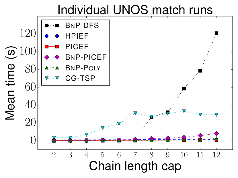
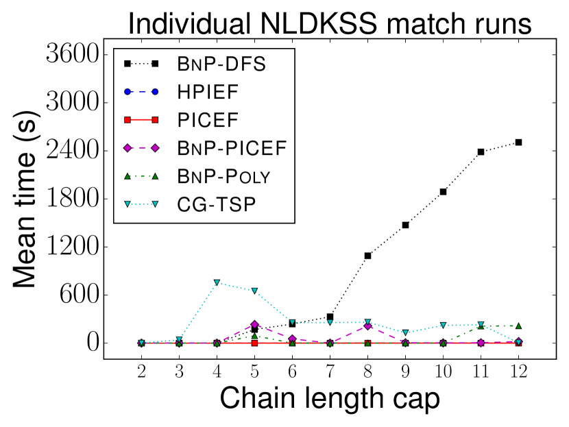
We now present results on real match run data from two fielded nationwide kidney exchanges: The United Network for Organ Sharing (UNOS) US-wide kidney exchange where the decisions are made by algorithms and software from Prof. Sandholm’s group, and the UK kidney exchange (NLDKSS) where the decisions are made by algorithms and software from Dr. Manlove’s group.333Due to privacy constraints on sharing real healthcare data, the UNOS and NLDKSS experimental runs were necessarily performed on different computers—one in the US and one in the UK. All runs within a figure were performed on the same machine, so relative comparisons of solvers within a figure are accurate. The UNOS instances used include all the match runs starting from the beginning of the exchange in October to January . The exchange has grown significantly during that time and chains have been incorporated. The match cadence has increased from once a month to twice a week; that keeps the number of altruists relatively small. On average, these instances have , , and . The NLDKSS instances cover the quarterly match runs during the period January –January . On average, these instances have , , and .
Figure 5 shows mean run times across all match runs for both exchanges; Appendix 12 gives additional statistics like minimum and maximum run times, as well as their standard deviations. Immediately obvious is that the non-compact formulations—BnP-DFS and CG-TSP—tend to scale poorly compared to our newer formulations. Interestingly, BnP-PICEF tends to perform worse than the base PICEF and HPIEF; we hypothesize that this is because branch-and-price-based methods are necessarily more “heavyweight” than standard IP techniques, and the small size of presently-fielded kidney exchange pools may not yet warrant this more advanced technique. Perhaps most critically, both PICEF and HPIEF clear real match runs in both exchanges within seconds.
In the NLDKSS results, the wide fluctuation in mean run time as the chain cap is varied can be explained by the small sample size of available NLDKSS instances, and the fact that the algorithms other than HPIEF and PICEF occasionally timed out at one hour. By contrast, each of the HPIEF and PICEF runs on NLDKSS instances took less than five seconds to complete. We also note that the LP relaxation of PICEF and HPIEF are very tight in practice; the LPR bound equaled the IP optimum for of the runs carried out on NLDKSS data.
We remark that the BnP-DCD model due to Klimentova et al. (2014) was run on all NLDKSS instances where the chain cap was equal to . Larger values of could not be tested since the current implementation of the model in our possession does not accept NDDs in the input. However for the case that the BnP-DCD model was the fastest for all NLDKSS instances.
Finally we note that the solver of Glorie et al. (2014) was executed on the NLDKSS instances with a chain cap of , for . It was found that on average the execution time was times slower than the fastest solver from among all the others executed on these instances as detailed at the beginning of Section 5. PICEF was the fastest solver on % of occasions.
5.2 Scaling experiments on realistic generated UNOS kidney exchange graphs
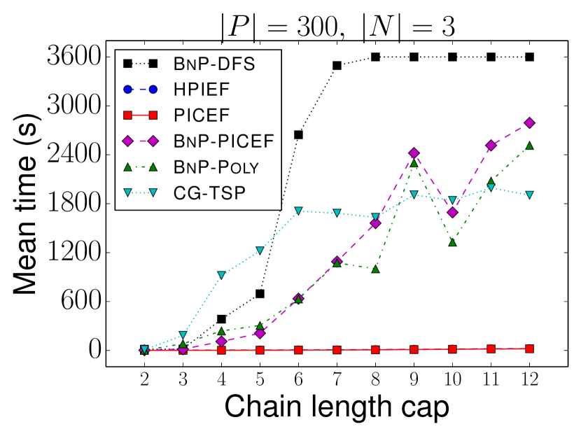
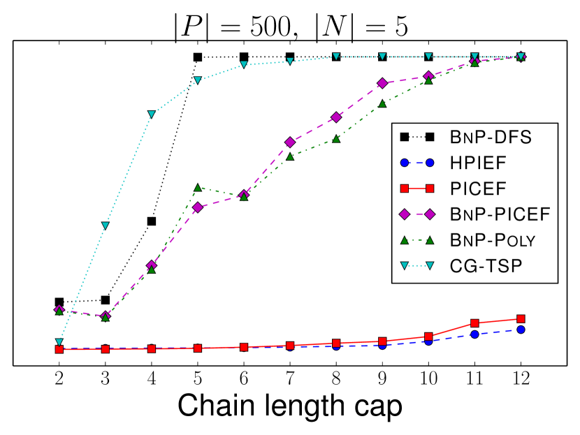
As motivated earlier in the paper, it is expected that kidney exchange pools will grow in size as (a) the idea of kidney exchange becomes more commonplace, and barriers to entry continue to drop, as well as (b) organized large-scale international exchanges manifest. Toward that end, in this section, we test solvers on generated compatibility graphs from a realistic simulator seeded by all historical UNOS data; the generator samples patient-donor pairs and NDDs with replacement, and draws arcs in the compatibility graph in accordance with UNOS’ internal arc creation rules.
Figure 6 gives results for increasing numbers of patient-donor pairs (each column), as well as increasing numbers of non-directed donors as a percentage of the number of patient-donor pairs (each row). As expected, as the number of patient-donor pairs increases, so too do run times for all solvers. Still, in each of the experiments, for each chain cap, both PICEF and HPIEF are on par or (typically) much faster—sometimes by orders of magnitude compared to other solvers. Appendix 12 gives these results in tabular form, including other statistics—minimum and maximum run times, as well as their standard deviations—that were not possible to show in Figure 6.
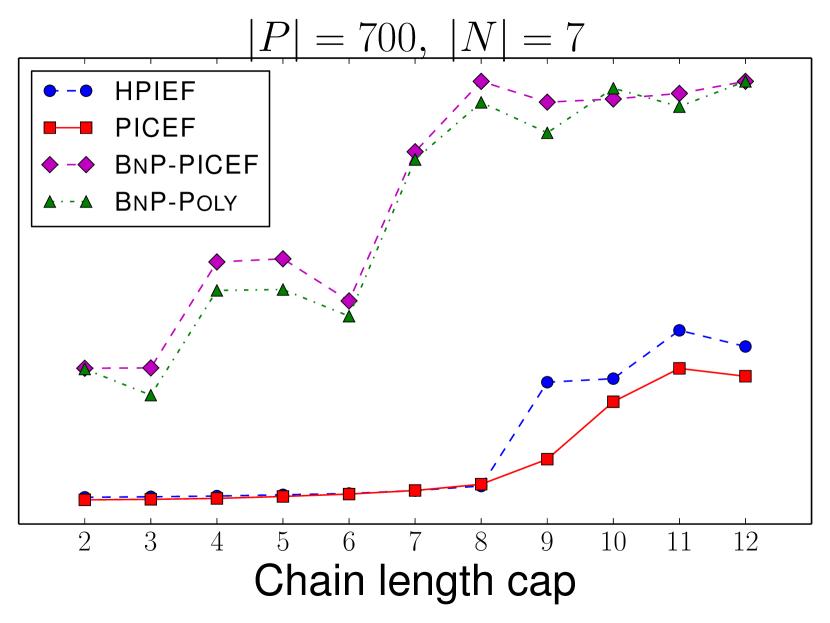
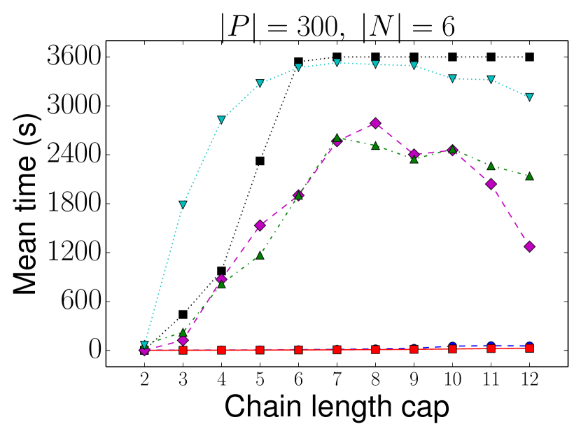
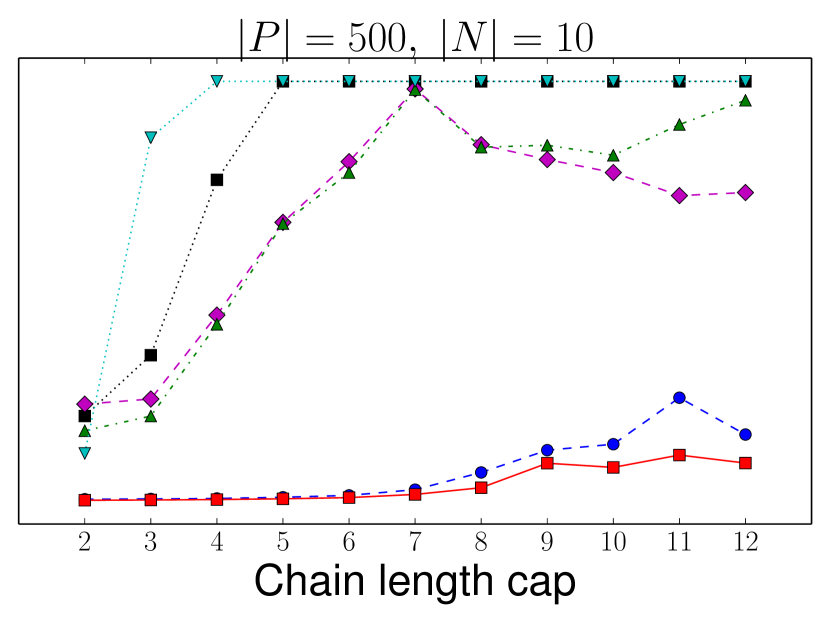
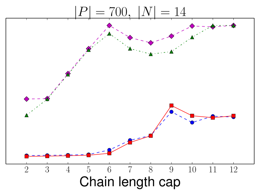
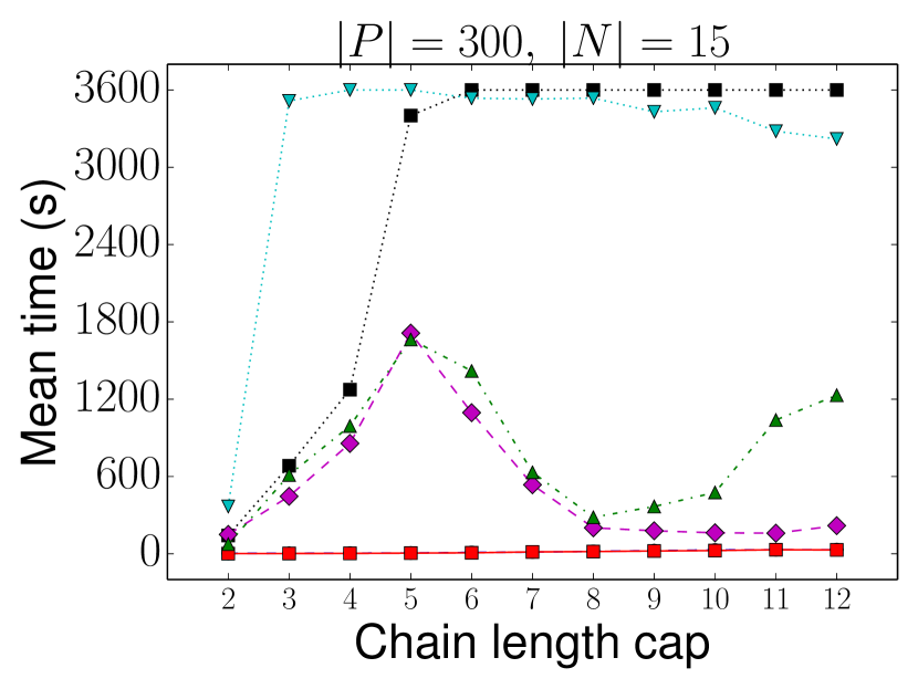
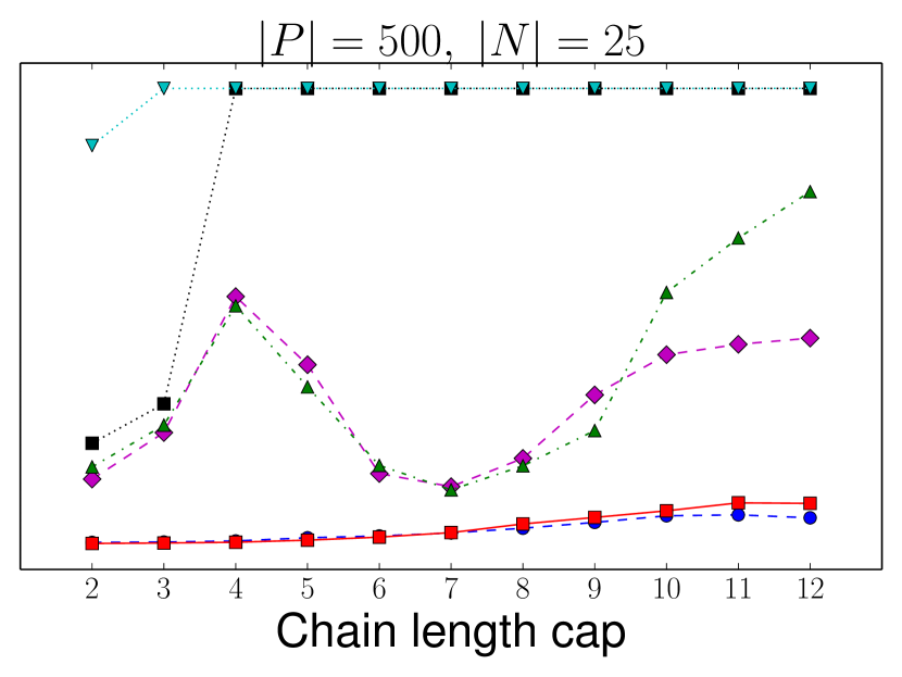
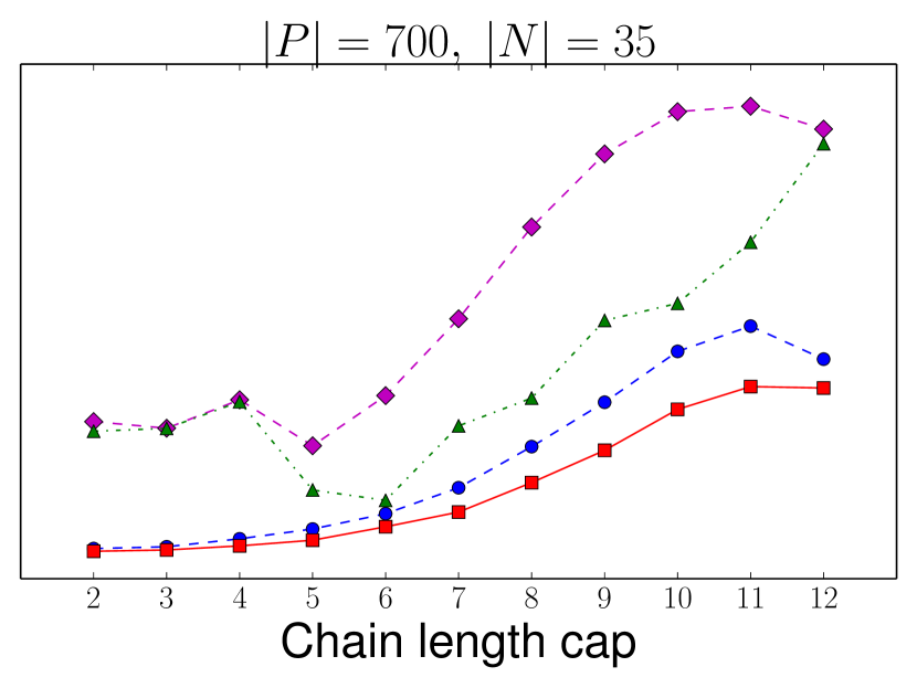
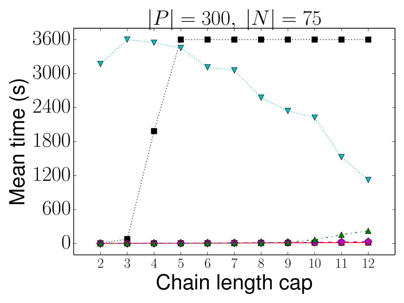
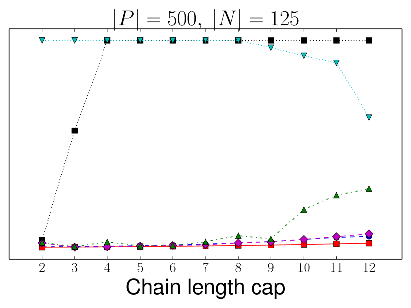
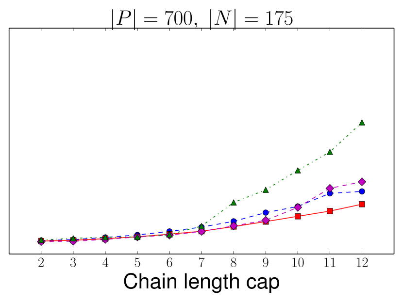
In addition to their increased scalability, we note two additional benefits of the PICEF and HPIEF models proposed in this paper: reduced variance in run time, and relative ease of implementation when compared to other state-of-the-art solution techniques. In both the real and simulated experimental results, we find that the run time of both the PICEF and HPIEF formulations is substantially less variable than the branch-and-price-based and constraint-generation-based IP solvers. While the underlying problem being solved is NP-hard, and thus will always present worst-case instances that take substantially longer than is typical to solve, the increased predictability of the run time of these models relative to other state-of-the-art solutions—including those that are presently fielded—is attractive. Second, we note that significant engineering effort is involved in the creation of custom branch-and-price and constraint-generation-based codes, while both PICEF and HPIEF are implemented with relative ease, relying on only a single call to a black box IP solver.
6 Failure-aware kidney exchange
Real-world exchanges all suffer to varying degrees from “last-minute” failures, where an algorithmic match or set of matches fails to move to transplantation. This can occur for a variety of reasons, including more extensive medical testing performed before a surgery, a patient or donor becoming too sick to participate, or a patient receiving an organ from another exchange or from the deceased donor waiting list.
To address these post-match arc failures, Dickerson et al. (2013) augments the standard model of kidney exchange to include a success probability for each arc in the graph. They show how to solve this model using branch and price, where the pricing problem is solved in time exponential in the chain and cycle cap. Prior compact formulations—and, indeed, prior “edge formulations” like those due to Abraham et al. (2007), Constantino et al. (2013), and Anderson et al. (2015)—are not expressive enough to allow for generalization to this model. Intuitively, while a single arc failure prevents an entire cycle from executing, chains are capable of incremental execution, yielding utility from the NDD to the first arc failure. Thus, the expected utility gained from an arc in a chain is dependent on where in the chain that arc is located, which is not expressed in those models.
6.1 PICEF for failure-aware matching
With only minor modification, PICEF allows for implementation of failure-aware kidney exchange, under the restriction that each arc is assumed to succeed with equal probability . While this assumption of equal probabilities is likely not true in practice, Dickerson et al. (2013) motivate why a fielded implementation of this model would potentially choose to equalize all failure probabilities: namely, so that already-sick patients—who will likely have higher failure rates—are not further marginalized by this model. Thus, given a single success probability , we can adjust the PICEF objective function to return the maximum expected weight matching as follows:
| (5a) | ||||
Objective (5a) is split into two parts: the utility received from arcs in chains, and the utility received from cycles. For the latter, a cycle of size has probability of executing; otherwise, it yields zero utility. For the former, if an arc is used at position in a chain, then it yields a fraction of its original weight—that is, the probability that the underlying chain will execute at least through its first arcs.
6.2 Failure-aware polynomial pricing for cycles
The initial failure-aware branch-and-price work by Dickerson et al. (2013) generalized the pricing strategy of Abraham et al. (2007), and thus suffered from a pricing problem that ran in time exponential in cycle and chain cap. Glorie et al. (2014) and Plaut et al. (2016a) discussed polynomial pricing algorithms for cycles—but not chains Plaut et al. (2016b)—in the deterministic case. Using the algorithm of Plaut et al. (2016a) as a subroutine, we present an algorithm which solves the failure-aware, or discounted, pricing problem for cycles in polynomial time, under the restriction that all arcs have equal success probability .
In the deterministic setting, the price of a cycle is , where is the weight of arc , and is the dual value of vertex in the LP. Glorie et al. (2014) show how the arc weights and dual values can be collapsed into just arc weights, and reduce the deterministic pricing problem to finding negative-weight cycles of length at most in a directed graph. In this section, we use “length” to denote the number of vertices in a cycle, not its weight.
The discounted price of a cycle is . Since the utility of an arc now depends on what cycle it ends up in, we cannot collapse arc weights and dual values without knowing the length of the cycle containing it.
With this motivation, we augment the algorithm to run iterations for each source vertex: one for each possible final cycle length. On each iteration, we know exactly how much arc weights will be worth in the final cycle, so we can reduce the discounted pricing problem to the deterministic pricing problem.
Pseudocode for the failure-aware cycle pricing algorithm is given by GetDiscountedPositivePriceCycles. Let and be the arc weights and dual values respectively in the original graph. The function GetNegativeCycles is the deterministic pricing algorithm due to Plaut et al. (2016a) which returns at least one negative cycle of length at most , or shows that none exist.
The algorithm of Plaut et al. (2016a) has complexity . Considering all possible cycle lengths brings the complexity of our algorithm to .
Theorem 6.1.
If there is a discounted positive price cycle in the graph, Algorithm 1 will return at least one discounted positive price cycle.
7 Conclusions & Future Research
In this paper, we addressed the tractable clearing of kidney exchanges with short cycles and long, but bounded, chains. This is motivated by kidney exchange practice, where chains are often long but bounded in length due to post-match arc failure. We introduced three IP formulations, two of which are compact, and favorably compared their LPRs to a state-of-the-art formulation with a tight relaxation. Then, on real data from the UNOS US nationwide exchange and the NLDKSS United Kingdom nationwide exchange, as well as on generated data, we showed that our new models outperform all other solvers on realistically-parameterized kidney exchange problems–often dramatically. We also explored practical extensions of our models, such as the use of branch and price for additional scalability, and an extension to the failure-aware kidney exchange case that more accurately mimics reality.
Beyond the immediate importance of more scalable static kidney exchange solvers for use in fielded exchanges, solvers like the ones presented in this paper are of practical importance in more advanced—and as yet unfielded—approaches to clearing kidney exchange. In reality, patients and donors arrive to and depart from the exchange dynamically over time Ünver (2010). Approaches to clearing dynamic kidney exchange often rely on solving the static problem many times Awasthi and Sandholm (2009); Dickerson et al. (2012); Anderson (2014); Dickerson and Sandholm (2015); Glorie et al. (2015); thus, faster static solvers result in better dynamic exchange solutions. Use of the techniques in this paper—or adaptations thereof—as subsolvers is of interest.
From a theoretical point of view, extending the comparison of LPRs to a complete ordering of all LPRs amongst models of kidney exchange—especially for different parameterizations of the underlying model, like the inclusion of chains or arc failures—would give insight as to which solver is best suited for an exchange running under a specific set of business constraints.
The authors would like to thank Ross Anderson, Kristiaan Glorie, Xenia Klimentova, Nicolau Santos, and Ana Viana for valuable discussions regarding this work and for making available their kidney exchange software for the purposes of conducting our experimental evaluation.
References
- (1)
- Abraham et al. (2007) David Abraham, Avrim Blum, and Tuomas Sandholm. 2007. Clearing Algorithms for Barter Exchange Markets: Enabling Nationwide Kidney Exchanges. In Proceedings of the ACM Conference on Electronic Commerce (EC). 295–304.
- Akbarpour et al. (2014) Mohammad Akbarpour, Shengwu Li, and Shayan Oveis Gharan. 2014. Dynamic Matching Market Design. In Proceedings of the ACM Conference on Economics and Computation (EC). 355.
- Alvelos et al. (2015) Filipe Alvelos, Xenia Klimentova, Abdur Rais, and Ana Viana. 2015. A compact formulation for maximizing the expected number of transplants in kidney exchange programs. In Journal of Physics: Conference Series, Vol. 616. IOP Publishing.
- Anderson (2014) Ross Anderson. 2014. Stochastic models and data driven simulations for healthcare operations. Ph.D. Dissertation. Massachusetts Institute of Technology.
- Anderson et al. (2015) Ross Anderson, Itai Ashlagi, David Gamarnik, and Alvin E Roth. 2015. Finding long chains in kidney exchange using the traveling salesman problem. Proceedings of the National Academy of Sciences 112, 3 (2015), 663–668.
- Ashlagi et al. (2015) Itai Ashlagi, Felix Fischer, Ian A Kash, and Ariel D Procaccia. 2015. Mix and Match: A strategyproof mechanism for multi-hospital kidney exchange. Games and Economic Behavior 91 (2015), 284–296.
- Ashlagi et al. (2012) Itai Ashlagi, David Gamarnik, Michael Rees, and Alvin E. Roth. 2012. The Need for (long) Chains in Kidney Exchange. NBER Working Paper No. 18202. (July 2012).
- Ashlagi et al. (2013) Itai Ashlagi, Patrick Jaillet, and Vahideh H. Manshadi. 2013. Kidney Exchange in Dynamic Sparse Heterogenous Pools. In Proceedings of the ACM Conference on Electronic Commerce (EC). 25–26.
- Ashlagi and Roth (2014) Itai Ashlagi and Alvin E Roth. 2014. Free riding and participation in large scale, multi-hospital kidney exchange. Theoretical Economics 9, 3 (2014), 817–863.
- Awasthi and Sandholm (2009) Pranjal Awasthi and Tuomas Sandholm. 2009. Online Stochastic Optimization in the Large: Application to Kidney Exchange. In Proceedings of the 21st International Joint Conference on Artificial Intelligence (IJCAI). 405–411.
- Barnhart et al. (1998) Cynthia Barnhart, Ellis Johnson, George Nemhauser, Martin Savelsbergh, and Pamela Vance. 1998. Branch-and-price: column generation for solving huge integer programs. Operations Research 46 (1998), 316–329.
- Biró et al. (2009) Péter Biró, David F Manlove, and Romeo Rizzi. 2009. Maximum weight cycle packing in directed graphs, with application to kidney exchange programs. Discrete Mathematics, Algorithms and Applications 1, 04 (2009), 499–517.
- Blum et al. (2015) Avrim Blum, John P. Dickerson, Nika Haghtalab, Ariel D. Procaccia, Tuomas Sandholm, and Ankit Sharma. 2015. Ignorance is Almost Bliss: Near-Optimal Stochastic Matching with Few Queries. In Proceedings of the ACM Conference on Economics and Computation (EC). 325–342.
- Blum et al. (2013) Avrim Blum, Anupam Gupta, Ariel D. Procaccia, and Ankit Sharma. 2013. Harnessing the Power of Two Crossmatches. In Proceedings of the ACM Conference on Electronic Commerce (EC). 123–140.
- Constantino et al. (2013) Miguel Constantino, Xenia Klimentova, Ana Viana, and Abdur Rais. 2013. New insights on integer-programming models for the kidney exchange problem. European Journal of Operational Research 231, 1 (2013), 57–68.
- Dickerson et al. (2012) John P. Dickerson, Ariel D. Procaccia, and Tuomas Sandholm. 2012. Dynamic Matching via Weighted Myopia with Application to Kidney Exchange. In AAAI Conference on Artificial Intelligence (AAAI). 1340–1346.
- Dickerson et al. (2013) John P. Dickerson, Ariel D. Procaccia, and Tuomas Sandholm. 2013. Failure-Aware Kidney Exchange. In Proceedings of the ACM Conference on Electronic Commerce (EC). 323–340.
- Dickerson and Sandholm (2015) John P. Dickerson and Tuomas Sandholm. 2015. FutureMatch: Combining Human Value Judgments and Machine Learning to Match in Dynamic Environments. In AAAI Conference on Artificial Intelligence (AAAI). 622–628.
- Ding et al. (2015) Yichuan Ding, Dongdong Ge, Simai He, and Christopher Ryan. 2015. A non-asymptotic approach to analyzing kidney exchange graphs. In Proceedings of the ACM Conference on Economics and Computation (EC). 257–258.
- Glorie et al. (2015) Kristiaan Glorie, Margarida Carvalho, Miguel Constantino, Paul Bouman, and Ana Viana. 2015. Robust Models for the Kidney Exchange Problem. (2015). Working paper.
- Glorie et al. (2014) Kristiaan M. Glorie, J. Joris van de Klundert, and Albert P. M. Wagelmans. 2014. Kidney Exchange with Long Chains: An Efficient Pricing Algorithm for Clearing Barter Exchanges with Branch-and-Price. Manufacturing & Service Operations Management (MSOM) 16, 4 (2014), 498–512.
- Hart et al. (2016) A. Hart, J. M. Smith, M. A. Skeans, S. K. Gustafson, D. E. Stewart, W. S. Cherikh, J. L. Wainright, G. Boyle, J. J. Snyder, B. L. Kasiske, and A. K. Israni. 2016. Kidney. American Journal of Transplantation (Special Issue: OPTN/SRTR Annual Data Report 2014) 16, Issue Supplement S2 (2016), 11–46.
- Klimentova et al. (2014) Xenia Klimentova, Filipe Alvelos, and Ana Viana. 2014. A New Branch-and-Price Approach for the Kidney Exchange Problem. In Computational Science and Its Applications (ICCSA-2014). Springer, 237–252.
- Mak-Hau (2015) Vicky Mak-Hau. 2015. On the kidney exchange problem: cardinality constrained cycle and chain problems on directed graphs: a survey of integer programming approaches. Journal of Combinatorial Optimization (2015), 1–25.
- Manlove and O’Malley (2015) David Manlove and Gregg O’Malley. 2015. Paired and Altruistic Kidney Donation in the UK: Algorithms and Experimentation. ACM Journal of Experimental Algorithmics 19, 1 (2015).
- Mattei and Walsh (2013) Nicholas Mattei and Toby Walsh. 2013. Preflib: A library for preferences. In Algorithmic Decision Theory. Lecture Notes in Computer Science, Vol. 8176. Springer, 259–270.
- Montgomery et al. (2006) Robert Montgomery, Sommer Gentry, William H Marks, Daniel S Warren, Janet Hiller, Julie Houp, Andrea A Zachary, J Keith Melancon, Warren R Maley, Hamid Rabb, Christopher Simpkins, and Dorry L Segev. 2006. Domino paired kidney donation: a strategy to make best use of live non-directed donation. The Lancet 368, 9533 (2006), 419–421.
- Pedroso (2014) João Pedro Pedroso. 2014. Maximizing Expectation on Vertex-Disjoint Cycle Packing. In Computational Science and Its Applications (ICCSA-2014). Springer, 32–46.
- Plaut et al. (2016a) Benjamin Plaut, John P. Dickerson, and Tuomas Sandholm. 2016a. Fast Optimal Clearing of Capped-Chain Barter Exchanges. In AAAI Conference on Artificial Intelligence (AAAI). 601–607.
- Plaut et al. (2016b) Benjamin Plaut, John P. Dickerson, and Tuomas Sandholm. 2016b. Hardness of the Pricing Problem for Chains in Barter Exchanges. CoRR abs/1606.00117 (2016).
- Rapaport (1986) F. T. Rapaport. 1986. The case for a living emotionally related international kidney donor exchange registry. Transplantation Proceedings 18 (1986), 5–9.
- Rees et al. (2009) Michael Rees, Jonathan Kopke, Ronald Pelletier, Dorry Segev, Matthew Rutter, Alfredo Fabrega, Jeffrey Rogers, Oleh Pankewycz, Janet Hiller, Alvin Roth, Tuomas Sandholm, Utku Ünver, and Robert Montgomery. 2009. A Nonsimultaneous, Extended, Altruistic-Donor Chain. New England Journal of Medicine 360, 11 (2009), 1096–1101.
- Roth et al. (2004) Alvin Roth, Tayfun Sönmez, and Utku Ünver. 2004. Kidney exchange. Quarterly Journal of Economics 119, 2 (2004), 457–488.
- Roth et al. (2005) Alvin Roth, Tayfun Sönmez, and Utku Ünver. 2005. Pairwise Kidney Exchange. Journal of Economic Theory 125, 2 (2005), 151–188.
- Roth et al. (2007) Alvin Roth, Tayfun Sönmez, and Utku Ünver. 2007. Efficient kidney exchange: Coincidence of wants in a market with compatibility-based preferences. American Economic Review 97 (2007), 828–851.
- Roth et al. (2006) Alvin Roth, Tayfun Sönmez, Utku Ünver, Frank Delmonico, and Susan L. Saidman. 2006. Utilizing list exchange and nondirected donation through ‘chain’ paired kidney donations. American Journal of Transplantation 6 (2006), 2694–2705.
- Toulis and Parkes (2015) Panos Toulis and David C. Parkes. 2015. Design and analysis of multi-hospital kidney exchange mechanisms using random graphs. Games and Economic Behavior 91, 0 (2015), 360–382.
- Ünver (2010) Utku Ünver. 2010. Dynamic kidney exchange. Review of Economic Studies 77, 1 (2010), 372–414.
- Vajda (1961) Steven Vajda. 1961. Mathematical Programming. Addison-Wesley.
8 Additional Proofs for the PIEF model
We now provide additional theoretical results pertaining to the position-indexed edge formulation (PIEF) model, and proofs to theoretical results stated in the main paper.
8.1 Validity of the PIEF model
Lemma 8.1.
Any assignment of values to the that respects the PIEF constraints yields a vertex-disjoint set of cycles of length no greater than .
Proof 8.2.
We show this by demonstrating that in each graph copy, the set of selected edges is either empty, or composes a single cycle of length no greater than .
Let be given such that at least one edge is selected in graph copy , and let be the highest position such that for some . Any selected edge at position in graph copy must point to , as otherwise the flow conservation constraint (1c) would be violated at vertex . Furthermore, there must be no more than one edge selected at position in graph copy , as otherwise the capacity constraint (1c) for vertex would be violated.
The flow conservation constraints (1b) ensure that we can follow a path backwards from the selected edge at position to a selected edge at position 1, and also that at most one edge is selected at each position. Since the edge at position 1 must start at vertex by the construction of , we have shown that graph copy contains a selected cycle beginning and ending at , and that this graph copy does not contain any other selected edges.
Constraint (1b) ensures that the vertex-disjointness condition is satisfied.
Lemma 8.3.
For any vertex-disjoint set of cycles of length no greater than , there is an assignment of values to the respecting the PIEF constraints.
Proof 8.4.
This assignment can be constructed trivially.
Theorem 8.5.
The PIEF model yields an optimal solution to the kidney exchange problem.
8.2 Proofs for the LPR of PIEF
The following lemma is used in the proof of Theorem 3.1, and its proof is included here for completeness.
Lemma 8.6.
Let a sequence of arcs in a directed graph be given, such that is a closed walk—that is, the target vertex of each arc is the source vertex of the following arc, and the sequence starts and ends at the same vertex. (It is permitted for an arc to appear more than once in .) Let be the multiset . Then we can partition into , where each is a set of arcs that form a cycle in .
Proof 8.7.
The following algorithm can be used to construct the set .
-
1.
Let .
-
2.
For each , let be the source vertex of .
-
3.
If the sequence contains no repeated vertices, then must be a cycle; go to step 5.
-
4.
Choose with , such that and all the are distinct for . The arcs form a cycle; remove these from and add the set of removed arcs to . (Observe that remains a closed walk). Re-index the arcs in the new, shorter as . Return to step 2.
-
5.
Add to and terminate.
See 3.1
Proof 8.8.
. Let be an optimal solution to the LPR of the cycle formulation, with objective value . We will construct a solution to the LPR of PIEF whose objective value is also . We translate the into an assignment of values to the in a natural way, as follows. For each , let be the index of the lowest-numbered vertex appearing in . Number the positions of arcs of in order as , beginning with the arc leaving .
For each vertex , each arc , and each position , let be the set of cycles in whose lowest-numbered vertex is and which contain at position . Let
This construction yields a solution which satisfies the PIEF constraints and has objective value .
. Let an optimal solution to the LPR of PIEF be given, with objective value . Our strategy is to begin by assigning zero to each cycle formulation variable , and to make a series of decreases in PIEF variables and corresponding increases in cycle formulation variables, ending when all of the PIEF variables are set to zero. We maintain three invariants after each such step. First, the sum of the PIEF and cycle formulation objective values remains . Second, the constraints of the relaxed PIEF are satisfied. Third, the following vertex capacity constraint—which combines the capacity constraints from the PIEF and the cycle formulation—is satisfied for each vertex.
If any of the PIEF variables takes a non-zero value, then we can select such that and . By the PIEF flow conservation constraints (1c), we can select a closed walk of at most arcs in such that for , and such that . Let be the smallest non-zero value taken by any of the .
By Lemma 8.6, the set of arc positions can be decomposed into a set of sets , such that for each we have that the arcs can be arranged to form a cycle; we denote this as . For each , we subtract from for each , and we add to . This transformation strictly decreases the count of variables that take a non-zero value. By repeatedly carrying out this step, we will reach a point where all of the variables take the value zero, and where the variables respect the cycle formulation constraints and give objective value .
9 Additional Proofs for the PICEF model
We now provide additional theoretical results pertaining to the position-indexed chain-edge formulation (PICEF) model, and proofs to theoretical results stated in the main paper.
9.1 Validity of the PICEF model
Lemma 9.1.
| (6) |
for all , yields a vertex-disjoint set chains of length no greater than .
Proof 9.2.
We say that arc is selected at position if and only if .
Our proof has three parts. We first give a procedure to construct a set of chains of length no greater than , where each chain in consists only of selected edges. We then show that these chains are vertex-disjoint, and that any selected edge appears in some chain in .
By constraint (4c), each has at most one selected outgoing arc. For each that has an outgoing arc , we begin to construct chain by letting —a sequence containing one edge. Vertex has at most one selected outgoing arc at position 2, by constraint (4d). If such an arc exists, we add it to our chain. We continue to add edges , until we reach such that a selected edge from at position does not exist. The chain will therefore be a path of selected edges at positions , where the length of can be no greater than since no variable in the model has position greater than . Add the chain to .
By constraint (4c), no vertex in can appear in two chains in . By constraint (4b), the same is true for vertices in . Hence, the chains in are vertex disjoint.
To complete the proof, we show that any selected edge must be part of one of these chains in . Let a variable taking the value 1 be given. By applying constraint (4d) repeatedly, we can see that there must exist be a path of length from an NDD to , containing only selected edges. Let be the chain starting at . Since no vertex in has two selected outgoing arcs, there must must exist a unique path of length from , and must therefore be the th edge of .
Lemma 9.3.
Any assignment of values to the and that respects the PICEF constraints yields a vertex-disjoint set cycles of length no greater than and chains no greater than .
Proof 9.4.
We call a cycle such that a selected cycle, and an arc such that for some a selected arc.
By (4b), the selected cycles are vertex disjoint. By Lemma 9.1 the selected arcs compose a set of vertex-disjoint chains, each of which has length bounded by (The conditions of the lemma are satisfied since constraint (4b) implies (6)).
It remains to show that no selected cycle shares a vertex with a selected arc. Suppose, to the contrary, that some selected cycle shares vertex with a selected arc . Vertex cannot be the target of , since constraint (4b) would be violated if appears both in selected cycle and as the target of selected arc . Hence for some . By constraint (4d), must be the target of another selected arc, . Therefore, appears in and is the target of , violating constraint (4b).
Lemma 9.5.
For any valid set of vertex-disjoint cycles and chains, there is an assignment of values to the and respecting the PICEF constraints.
Proof 9.6.
This assignment can be constructed trivially.
Theorem 9.7.
The PICEF model yields an optimal solution to the kidney exchange problem.
9.2 Proofs for the LPR of PICEF
See 4.1
Proof 9.8.
. Consider an optimal solution to the LPR of the cycle formulation. We show how to construct an equivalent (optimal) solution to the LPR of PICEF. For , we transfer the value of directly from the cycle formulation solution to the PICEF solution. For each and each , let
This solution has the same objective value as the cycle formulation solution, and satisfies the constraints of the LPR of PICEF.
. Figure 7 shows a graph for which is strictly greater (i.e., worse) than . Let and . In this instance, and .
In the cycle formulation, this instance has no admissible cycles, and the only admissible chains are , , and their prefixes. Since the longest chain has length 3 and any the sum of chain-variables containing vertex 1 may not exceed 1, we can see that the optimal objective value to the LPR of the cycle formulation is 3.
We can achieve an objective value of to the LPR of PICEF, by letting .
See 4.2
Proof 9.9.
We give a family of graphs, parameterised by and , for which is strictly greater than . Given a constant cycle cap of and a chain cap of (which can effectively be infinite, if ), the graphs are constructed as follows. For , create a cycle such that for each ; the cycle is otherwise disjoint from the rest of the graph. Connect a single altruist to ; the altruist is otherwise disjoint from the rest of the graph. Figure 8 visualizes the constructed graph.
The maximum cardinality disjoint packing of cycles of length at most and chains of length at most is the unique chain . Thus, , where is the optimal objective value to the integer program. Indeed, there are no legal cycles of length at most in the graph, and at most one chain can be in any feasible solution due to the shared altruist , so the (unique, by construction) longest chain is optimal.
The LPR of the PICEF representation of this instance will assign weight of to each edge in the graph, for a total objective of .
The LPR of the cycle formulation representation will create variables for each feasible cycle and chain in the graph. There are no feasible cycles in the graph. All chains in the graph share the edge ; thus all chains intersect and all chains contain . Thus, the sole binding constraint in the LPR of the cycle formulation is that the altruist node appears in at most one chain. For chain decision variables , this problem can be rewritten as
This constraint matrix is totally unimodular, and thus the LP optimum is integral (and is the IP optimum, or ).
The ratio of to is thus
which can be made arbitrarily large by increasing .
10 Hybrid Formulation
10.1 Description of the HPIEF model
In this section, we present a compact generalization of the PIEF model to kidney exchange graphs with non-directed donors. This stands in contrast to the the PICEF formulation, which has polynomial counts of constraints and edge variables, but an exponential number of cycle variables. By replacing the cycle variables in PICEF with the variables from PIEF and modifying the constraints accordingly, we can create a compact formulation, the hybrid PIEF (HPIEF). Let the variables and the index set be defined as in PIEF. Let the variables and the index set be defined as in PICEF. The HPIEF integer program is as follows.
10.2 Validity of the HPIEF model
Lemma 10.1.
Any assignment of values to the and that respects the HPIEF constraints yields a vertex-disjoint set cycles of length no greater than and chains no greater than .
Proof 10.2.
(Sketch.) Clearly, if the HPIEF constraints are satisfied then the PIEF constraints (1b-1d) are satisfied also. Therefore, by Theorem 8.1, the edges selected by the form a vertex-disjoint set of cycles of length no greater than .
By Lemma 9.1, the selected arcs compose a set of vertex-disjoint chains, each of which has length bounded by .
It remains to show that the selected cycles and chains are vertex-disjoint. This can be showed straightforwardly, along similar lines to the proof for Theorem 9.3.
Lemma 10.3.
For any valid set of vertex-disjoint cycles and chains, there is an assignment of values to the and respecting the HPIEF constraints.
Proof 10.4.
This assignment can be constructed trivially.
Theorem 10.5.
The HPIEF model yields an optimal solution to the kidney exchange problem.
10.3 LPR comparison of HPIEF and PICEF
Theorem 10.6.
The proof is similar to the proof for Theorem 3.1, and is therefore omitted.
11 Additional Background and Proofs for Failure-Aware the PICEF Model
In this section, we provide a proof of correctness of Algorithm 1—which implements polynomial-time pricing of cycles for branch and price in the augmented failure-aware PICEF model—and discuss by way of counterexample why the basic deterministic polynomial-time cycle pricing algorithms of Glorie et al. (2014) and Plaut et al. (2016a) cannot be directly used for this case.
11.1 Proof of Theorem 6.1
See 6.1
Proof 11.1.
Let be a discounted positive price cycle. Then . Therefore . Then by definition of , we have .
This implies that is a negative cycle in on the iteration of Algorithm 1. By the correctness of GetNegativeCycles, if there is a negative cycle in the graph, GetNegativeCycles will return at least one negative cycle of length at most .
Let be a returned cycle. Since is negative in on the iteration, we have . Therefore .
Since by the correctness of GetNegativeCycles, we have . Because all arc weights in the original graph are nonnegative, . Therefore . Then , so is indeed discounted positive price.
Therefore Algorithm 1 returns at least one discounted positive price cycle.
11.2 Insufficiency of previous algorithms for the failure-aware pricing problem
The pricing problem in the deterministic context, where post-match failures are not considered, is known to be solvable in polynomial time for cycles Glorie et al. (2014); Plaut et al. (2016a) but not chains Plaut et al. (2016b). In Section 6.2, we presented Algorithm 1, a polynomial-time algorithm for the pricing problem for cycles in the failure-aware context, for uniform success probability. In this section, we show how the basic algorithm for the deterministic pricing problem is not sufficient for the failure-aware context.
The algorithm for the deterministic setting initiates a Bellman-Ford style search to find negative cycles. Bellman-Ford is run times: on each iteration a different vertex representing a donor-patient pair is the source. After Bellman-Ford has been run from the source for steps, suppose there is a path from to some vertex with weight , and there is an arc from back to with weight . If , then is a negative cycle Glorie et al. (2014); Plaut et al. (2016a).
For consistency, in this section we discuss finding discounted negative price cycles, which is trivially equivalent to finding discounted positive price cycles by reversing the signs on all arc weights and dual values. Therefore, we are looking for cycles satisfying .
Consider a straightforward modification to the algorithm from the deterministic setting, where each path now separately remembers its accumulated sum of dual values, sum of arc weights, and length. All of these can be easily recorded during the Bellman-Ford update step without altering the algorithm’s complexity.
The issue arises when comparing paths. Figure 9 gives an example of this. Consider running Bellman-Ford with as the source and . The path is preferable to , since we will end with the -cycle which has weight . However, suppose , and we removed the arc . Then is no longer a cycle, and the path will have weight , assuming is large and is not close to . However, the path would lead to a discounted negative cycle with weight . The algorithm from the deterministic setting cannot compare two paths without knowing the final cycle length.
12 Tabulated experimental results
In this section, we restate the experimental results shown in Figures 5 and 6 of Section 5 in the body of the paper, but now including statistics that were not possible to show in that figure.
UNOS match runs.
| Method | ||||||||||||
|---|---|---|---|---|---|---|---|---|---|---|---|---|
| PICEF | Mean | |||||||||||
| Stdev | ||||||||||||
| Min | ||||||||||||
| Max | ||||||||||||
| HPIEF | Mean | |||||||||||
| Stdev | ||||||||||||
| Min | ||||||||||||
| Max | ||||||||||||
| BnP-Poly | Mean | |||||||||||
| Stdev | ||||||||||||
| Min | ||||||||||||
| Max | ||||||||||||
| CG-TSP | Mean | |||||||||||
| Stdev | ||||||||||||
| Min | ||||||||||||
| Max | ||||||||||||
| BnP-DFS | Mean | |||||||||||
| Stdev | ||||||||||||
| Min | ||||||||||||
| Max | ||||||||||||
| BnP-PICEF | Mean | |||||||||||
| Stdev | ||||||||||||
| Min | ||||||||||||
| Max |
NLDKSS match runs.
| Method | ||||||||||||
|---|---|---|---|---|---|---|---|---|---|---|---|---|
| PICEF | Mean | |||||||||||
| Stdev | ||||||||||||
| Min | ||||||||||||
| Max | ||||||||||||
| HPIEF | Mean | |||||||||||
| Stdev | ||||||||||||
| Min | ||||||||||||
| Max | ||||||||||||
| BnP-Poly | Mean | |||||||||||
| Stdev | ||||||||||||
| Min | ||||||||||||
| Max | ||||||||||||
| CG-TSP | Mean | |||||||||||
| Stdev | ||||||||||||
| Min | ||||||||||||
| Max | ||||||||||||
| BnP-DFS | Mean | |||||||||||
| Stdev | ||||||||||||
| Min | ||||||||||||
| Max | ||||||||||||
| BnP-PICEF | Mean | |||||||||||
| Stdev | ||||||||||||
| Min | ||||||||||||
| Max |
| Method | ||||||||||||
|---|---|---|---|---|---|---|---|---|---|---|---|---|
| PICEF | Mean | |||||||||||
| Stdev | ||||||||||||
| Min | ||||||||||||
| Max | ||||||||||||
| HPIEF | Mean | |||||||||||
| Stdev | ||||||||||||
| Min | ||||||||||||
| Max | ||||||||||||
| BnP-Poly | Mean | |||||||||||
| Stdev | ||||||||||||
| Min | ||||||||||||
| Max | ||||||||||||
| BnP-PICEF | Mean | |||||||||||
| Stdev | ||||||||||||
| Min | ||||||||||||
| Max |