\SetBgContents

Bifurcation analysis of a stochastically driven limit cycle

Maximilian Engel Zentrum Mathematik der TU München, Boltzmannstr. 3, D-85748 Garching bei München    Jeroen S.W. Lamb Department of Mathematics, Imperial College London, 180 Queen’s Gate, London SW7 2AZ, United Kingdom    Martin Rasmussen22footnotemark: 2
(February 29, 2024)
Abstract

We establish the existence of a bifurcation from an attractive random equilibrium to shear-induced chaos for a stochastically driven limit cycle, indicated by a change of sign of the first Lyapunov exponent. This addresses an open problem posed by Kevin Lin and Lai-Sang Young in [21, 30], extending results by Qiudong Wang and Lai-Sang Young [28] on periodically kicked limit cycles to the stochastic context.


Key words. Furstenberg–Khasminskii formula, Lyapunov exponent, Random dynamical system, shear-induced chaos, stochastic bifurcation

Mathematics Subject Classification (2010). 37D45, 37G35, 37H10, 37H15.


1 Introduction

We consider the following model of a stochastically driven limit cycle

dy=αydt+σi=1mfi(ϑ)dWti,dϑ=(1+by)dt,d𝑦absent𝛼𝑦d𝑡𝜎superscriptsubscript𝑖1𝑚subscript𝑓𝑖italic-ϑdsuperscriptsubscript𝑊𝑡𝑖ditalic-ϑabsent1𝑏𝑦d𝑡\displaystyle\begin{array}[]{r@{\;\,=\;\,}l}\mathrm{d}y&-\alpha y\,\mathrm{d}t+\sigma\sum_{i=1}^{m}f_{i}(\vartheta)\circ\mathrm{d}W_{t}^{i}\,,\\ \mathrm{d}\vartheta&(1+by)\,\mathrm{d}t\ \,,\end{array} (1.3)

where (y,ϑ)×𝕊1𝑦italic-ϑsuperscript𝕊1(y,\vartheta)\in\mathbb{R}\times\mathbb{S}^{1} are cylindrical amplitude-phase coordinates, m𝑚m\in\mathbb{N}, and Wtisuperscriptsubscript𝑊𝑡𝑖W_{t}^{i} for i{1,,m}𝑖1𝑚i\in\{1,\dots,m\}, denote independent one-dimensional Brownian motions entering the equation as noise of Stratonovich type. In the absence of noise (σ=0𝜎0\sigma=0), the ODE (1.3) has a globally attracting limit cycle at y=0𝑦0y=0 if α>0𝛼0\alpha>0. In the presence of noise (σ0𝜎0\sigma\neq 0), the amplitude is driven by phase-dependent noise. The real parameter b𝑏b induces shear: if b0𝑏0b\neq 0, the phase velocity dϑdtditalic-ϑd𝑡\frac{\mathrm{d}\vartheta}{\mathrm{d}t} depends on the amplitude y𝑦y.

The stable limit cycle turns into a random attractor if σ0𝜎0\sigma\not=0. The main question we address in this paper concerns the nature of this random attractor. The crucial quantity is the sign of the first Lyapunov exponent λ1subscript𝜆1\lambda_{1} with respect to the invariant measure associated to the random attractor. In essence, λ1subscript𝜆1\lambda_{1} is the dominant infinitesimal asymptotic expansion rate of almost all trajectories.

To facilitate the analysis, we choose fi:𝕊1[0,1):subscript𝑓𝑖similar-to-or-equalssuperscript𝕊101f_{i}:\mathbb{S}^{1}\simeq[0,1)\to\mathbb{R} such that

i=1mfi(ϑ)2=1for all ϑ𝕊1.formulae-sequencesuperscriptsubscript𝑖1𝑚superscriptsubscript𝑓𝑖superscriptitalic-ϑ21for all italic-ϑsuperscript𝕊1\sum_{i=1}^{m}f_{i}^{\prime}(\vartheta)^{2}=1\ \quad\text{for all }\,\vartheta\in\mathbb{S}^{1}\,. (1.4)

If m2𝑚2m\geq 2, then the functions are assumed to be smooth. The simplest example is given by

m=2,f1(ϑ)=cos(ϑ),f2(ϑ)=sin(ϑ).formulae-sequence𝑚2formulae-sequencesubscript𝑓1italic-ϑitalic-ϑsubscript𝑓2italic-ϑitalic-ϑm=2,\quad f_{1}(\vartheta)=\cos(\vartheta),\quad f_{2}(\vartheta)=\sin(\vartheta)\,. (1.5)

For m=1𝑚1m=1, condition (1.4) cannot be satisfied for all ϑ𝕊1italic-ϑsuperscript𝕊1\vartheta\in\mathbb{S}^{1}. Hence, we choose f:=f1:𝕊1[0,1):assign𝑓subscript𝑓1similar-to-or-equalssuperscript𝕊101f:=f_{1}:\mathbb{S}^{1}\simeq[0,1)\to\mathbb{R} to be continuous and piecewise linear with constant absolute value of the derivative almost everywhere. The simplest example is given by

f(ϑ)={ϑifϑ12,(1ϑ)ifϑ12.𝑓italic-ϑcasesitalic-ϑifitalic-ϑ121italic-ϑifitalic-ϑ12f(\vartheta)=\begin{cases}\vartheta\ &\text{if}\ \vartheta\leq\frac{1}{2}\,,\\ (1-\vartheta)\ &\text{if}\ \vartheta\geq\frac{1}{2}\,.\end{cases} (1.6)

With such choices of the amplitude-phase coupling we obtain the following bifurcation result.

Theorem 1.1.

Consider the SDE (1.3) with fisubscript𝑓𝑖f_{i}, i=1,,m𝑖1𝑚i=1,\dots,m, satisfying condition (1.4). Then there is c00.2823subscript𝑐00.2823c_{0}\approx 0.2823 such that for all α>0𝛼0\alpha>0 and b0𝑏0b\neq 0 the number σ0(α,b)=α3/2c01/2|b|>0subscript𝜎0𝛼𝑏superscript𝛼32superscriptsubscript𝑐012𝑏0\sigma_{0}(\alpha,b)=\frac{\alpha^{3/2}}{c_{0}^{1/2}\left|b\right|}>0 is the unique value of σ𝜎\sigma where the top Lyapunov exponent λ1(α,b,σ)subscript𝜆1𝛼𝑏𝜎\lambda_{1}(\alpha,b,\sigma) of (1.3) changes its sign. In more detail, we have

λ1(α,b,σ){<0if 0<σ<σ0(α,b),=0ifσ=σ0(α,b),>0ifσ>σ0(α,b).subscript𝜆1𝛼𝑏𝜎casesotherwiseformulae-sequenceabsent0if 0𝜎subscript𝜎0𝛼𝑏otherwiseformulae-sequenceabsent0if𝜎subscript𝜎0𝛼𝑏otherwiseformulae-sequenceabsent0if𝜎subscript𝜎0𝛼𝑏\lambda_{1}(\alpha,b,\sigma)\begin{cases}&<0\quad\text{if}\ 0<\sigma<\sigma_{0}(\alpha,b)\,,\\ &=0\quad\text{if}\ \sigma=\sigma_{0}(\alpha,b)\,,\\ &>0\quad\text{if}\ \sigma>\sigma_{0}(\alpha,b)\,.\end{cases}

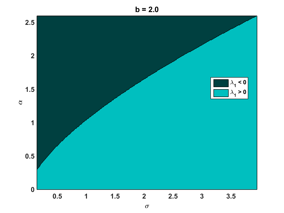
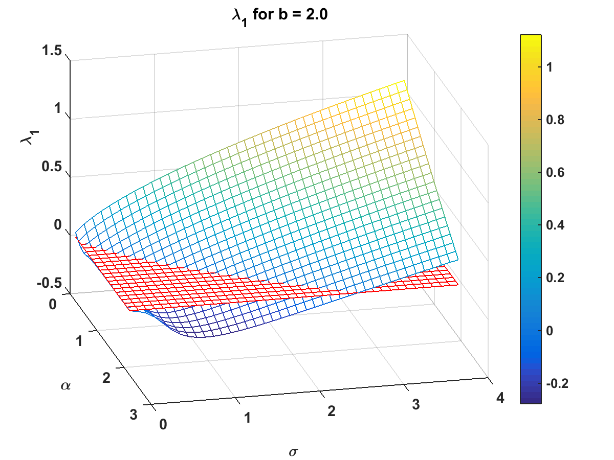
As long as b,σ0𝑏𝜎0b,\sigma\neq 0, the amplitude variable y𝑦y can be rescaled so that the shear parameter becomes equal to 111 and the effective noise-amplitude becomes σb𝜎𝑏\sigma b. Hence, the above result also holds with the roles of σ𝜎\sigma and b𝑏b interchanged. The fact that σ0(α,b)subscript𝜎0𝛼𝑏\sigma_{0}(\alpha,b) is an increasing function of α𝛼\alpha is illustrated in Figure 1. Figure 1(a) depicts λ1subscript𝜆1\lambda_{1} as a function of α𝛼\alpha and σ𝜎\sigma for fixed b=2𝑏2b=2. Figure 1(b) displays the corresponding areas of positive and negative top Lyapunov exponent in the (σ,α)𝜎𝛼(\sigma,\alpha)-parameter space where λ1=0subscript𝜆10\lambda_{1}=0 along the curve {(σ0(α,2),α)}subscript𝜎0𝛼2𝛼\{(\sigma_{0}(\alpha,2),\alpha)\} separating the two areas. If σ=0𝜎0\sigma=0, we clearly have λ1=0subscript𝜆10\lambda_{1}=0 for all α>0𝛼0\alpha>0. The case α=0𝛼0\alpha=0 is obviously not of any interest in our model.
Refer to caption
(a)
Refer to caption
(b)
Figure 1: In Figure 1(a) we depict the top Lyapunov exponent λ1subscript𝜆1\lambda_{1}, computed using (2.12), as a function of α𝛼\alpha and σ𝜎\sigma for fixed b=2𝑏2b=2. The red mesh demarcates the level λ1=0subscript𝜆10\lambda_{1}=0. Figure 1(b) shows the corresponding areas of positive and negative λ1subscript𝜆1\lambda_{1} in the (σ,α)𝜎𝛼(\sigma,\alpha)-parameter space being separated by the curve {(σ0(α,2),α)}subscript𝜎0𝛼2𝛼\{(\sigma_{0}(\alpha,2),\alpha)\}. The picture doesn’t display σ=0𝜎0\sigma=0: in this case, λ1=0subscript𝜆10\lambda_{1}=0 for all α>0𝛼0\alpha>0.

If the top Lyapunov exponent is negative, it turns out that the (weak) random point attractor is an attracting random equilibrium, i.e. its fibers are singletons almost surely. Properties of random attractors with positive top Lyapunov exponents are not yet well understood, apart from the fact that such attractors are not random equilibria. They are sometimes referred to as random strange attractors [19, 29]. Theorem 1.1 confirms numerical results by Lin & Young [21] for a very similar model. The mechanism, whereby a combination of shear and noise causes stretching and folding leading to a positive Lyapunov exponent, was coined with the term shear-induced chaos by Lin & Young. Wang & Young [27, 28] and Ott & Stenlund [24] have demonstrated analytically the validity of this mechanism in the case of periodically kicked limit cycles, including probabilistic characterizations of the dynamics. An analytical proof of shear-induced chaos in the stochastic setting, as presented in this paper, had remained an open problem.

The results of this paper are part of a larger effort to develop a bifurcation theory of random dynamical systems. Earlier attempts to develop such a theory (notably by Ludwig Arnold, Peter Baxendale and coworkers [2, 3, 5, 25] in the 1990s) led to notions of so-called phenomenological (or ”P”) bifurcations and dynamical (or ”D”) bifurcations, but there is growing evidence that these paradigms do not suffice to capture the intricacies of bifurcation in random dynamical systems [1, 8, 17, 31]. In the absence of a consensus on useful characterisations of the dynamics of random systems and bifurcations in this context, much of the current research inevitably focusses on the detailed analysis of relatively elementary examples, to generate insights and guidance towards the further development of a more general theory.

In one-dimensional SDEs, negative Lyapunov exponents and attractive random equilibria prevail [9]. Random strange attractors can only arise in dimension two and higher and up to now, little research has been devoted to such attractors. In contrast, the existence of attractive random equilibria (also referred to as synchronization, with reference to the corresponding dynamics of sets of initial conditions) has been studied well, also in higher dimensions [4, 12, 18, 22, 23].

The main technical challenge addressed in this paper is to establish the existence of positive top Lyapunov exponents. Most rigorous results on Lyapunov exponents (and random dynamical systems) are obtained for one-dimensional SDEs, in which case the analysis of Lyapunov exponents significantly simplifies due to the fact that all derivatives commute. It is difficult in general to obtain lower bounds for the top Lyapunov exponent in higher dimensions due to the subadditivity property of matrices, cf. [30]. Thus, the analytical demonstration of positive Lyapunov exponents for noisy systems has been achieved only in certain special cases, like for equilibria [13], simple time-discrete models as in [20] or under special circumstances that allow for the use of stochastic averaging [6, 7]. In our setting, condition (1.4) is crucial to establish rigorous lower bounds on the top Lyapunov exponent λ1subscript𝜆1\lambda_{1}.

Another prototypical open problem in dimension two is the stochastic Hopf bifurcation, concerning the characterisation of dynamics and bifurcations in parametrized families of SDEs that in the deterministic (noise-free) limit display a Hopf bifurcation. A (deterministic) Hopf bifurcation occurs if, by the variation of a model parameter, an asymptotically stable equilibrium loses stability under the emission of a small attracting limit cycle. Numerical studies [29] suggest that the mechanism of shear-induced chaos is at play also in stochastic Hopf bifurcations, but while analytical proofs of parameter regimes with negative top Lyapunov exponents are within reach [10, 11], until now, there are no rigorous results concerning the existence of parameter regimes with positive top Lyapunov exponents in this context. The results of this paper may well be relevant to shed more light on this problem.

The remainder of the paper is organized as follows. Section 2 provides the analysis of Lyapunov exponents for our model: Subsection 2.1 introduces the model on the cylinder within the framework of random dynamical systems and establishes the necessary theoretical concepts. Subsection 2.2 introduces the Furstenberg–Khasminskii forumula for the top Lyapunov exponent and in Subsection 2.3, we derive a formula for the top Lyapunov exponent λ1subscript𝜆1\lambda_{1}. The main result concerning the change of sign of λ1subscript𝜆1\lambda_{1} is proven in Section 3 and its consequences are discussed. We give illustrations of λ1subscript𝜆1\lambda_{1} in dependence on the parameters and confirm a scaling conjecture by Lin and Young. We conclude with a short summary in Section 4.

2 Analysis of the top Lyapunov exponent

2.1 Lyapunov exponents for random dynamical systems

Consider the stochastic differential equation of Stratonovich type (1.3). We assume that fi:[0,1]:subscript𝑓𝑖01f_{i}:[0,1]\to\mathbb{R}, i=1,,m𝑖1𝑚i=1,\dots,m, are Lipschitz continuous functions with f(0)=f(1)𝑓0𝑓1f(0)=f(1) (smooth if m2𝑚2m\geq 2 and piecewise linear if m=1𝑚1m=1), and the three parameters fulfill α>0𝛼0\alpha>0, σ>0𝜎0\sigma>0 and b𝑏b\in\mathbb{R}. Note that the equation reads the same in Itô form according to the Itô–Stratonovich conversion formula.

Since the drift and diffusion coefficients are Lipschitz continuous and satisfy linear growth conditions, the SDE (1.3) generates a continuous random dynamical system (θ,φ)𝜃𝜑(\theta,\varphi) [2, Definition 1.1.2] consisting of the following:

  1. (i)

    A model of the noise on the probability space Ω:=C0(,)={ωC(,):ω(0)=0}assignΩsubscript𝐶0conditional-set𝜔𝐶𝜔00\Omega:=C_{0}(\mathbb{R},\mathbb{R})=\{\omega\in C(\mathbb{R},\mathbb{R}):\omega(0)=0\} with Borel σ𝜎\sigma-algebra \mathcal{F} and two-sided Wiener measure \mathbb{P}, formalized as the family (θt)tsubscriptsubscript𝜃𝑡𝑡(\theta_{t})_{t\in\mathbb{R}} of \mathbb{P}-preserving shift maps given by (θtω)(s)=ω(s+t)ω(t)subscript𝜃𝑡𝜔𝑠𝜔𝑠𝑡𝜔𝑡(\theta_{t}\omega)(s)=\omega(s+t)-\omega(t).

  2. (ii)

    A model of the system perturbed by noise formalized as a cocycle φ𝜑\varphi over θ𝜃\theta of mappings of ×𝕊1superscript𝕊1\mathbb{R}\times\mathbb{S}^{1}, i.e. φ𝜑\varphi is a (0+)(×𝕊1)tensor-productsuperscriptsubscript0superscript𝕊1\mathcal{B}(\mathbb{R}_{0}^{+})\otimes\mathcal{F}\otimes\mathcal{B}(\mathbb{R}\times\mathbb{S}^{1})-measurable mapping

    φ:0+×Ω×(×𝕊1)×𝕊1,(t,ω,x)φ(t,ω)x,:𝜑formulae-sequencesuperscriptsubscript0Ωsuperscript𝕊1superscript𝕊1maps-to𝑡𝜔𝑥𝜑𝑡𝜔𝑥\varphi:\mathbb{R}_{0}^{+}\times\Omega\times(\mathbb{R}\times\mathbb{S}^{1})\to\mathbb{R}\times\mathbb{S}^{1},\quad(t,\omega,x)\mapsto\varphi(t,\omega)x,

    such that (t,x)φ(t,ω)xmaps-to𝑡𝑥𝜑𝑡𝜔𝑥(t,x)\mapsto\varphi(t,\omega)x is continuous for every ωΩ𝜔Ω\omega\in\Omega and which satisfies

    φ(0,ω)=idandφ(t+s,ω)=φ(t,θsω)φ(s,ω) for all ωΩ and t,s0+.formulae-sequence𝜑0𝜔idandformulae-sequence𝜑𝑡𝑠𝜔𝜑𝑡subscript𝜃𝑠𝜔𝜑𝑠𝜔formulae-sequence for all 𝜔Ω and 𝑡𝑠superscriptsubscript0\varphi(0,\omega)=\operatorname{id}\quad\text{and}\quad\varphi(t+s,\omega)=\varphi(t,\theta_{s}\omega)\circ\varphi(s,\omega)\quad\text{ for all }\omega\in\Omega\text{ and }t,s\in\mathbb{R}_{0}^{+}\,.

The random dynamical system (θ,φ)𝜃𝜑(\theta,\varphi) induced by (1.3) is also a skew product flow Θ=(θ,φ)Θ𝜃𝜑\Theta=(\theta,\varphi), which is a measurable dynamical system on the extended phase space Ω×XΩ𝑋\Omega\times X. The skew product flow ΘΘ\Theta possesses an ergodic invariant Markov measure μ𝜇\mu which is associated to the unique invariant measure (also called stationary measure) for the corresponding Markov semigroup. Their existence follows from the same considerations as in [21].

Fundamental for stochastic bifurcation theory is Oseledets’ Multiplicative Ergodic Theorem, which implies the existence of Lyapunov exponents describing stability properties of a differentiable random dynamical system. The random dynamical system (θ,φ)𝜃𝜑(\theta,\varphi) is called Cksuperscript𝐶𝑘C^{k} if φ(t,ω)Ck𝜑𝑡𝜔superscript𝐶𝑘\varphi(t,\omega)\in C^{k} for all t0+𝑡superscriptsubscript0t\in\mathbb{R}_{0}^{+} and ωΩ𝜔Ω\omega\in\Omega. In the situation of the Stratonovich SDE

dXt=f0(Xt)dt+i=1mfj(Xt)dWtjdsubscript𝑋𝑡subscript𝑓0subscript𝑋𝑡d𝑡superscriptsubscript𝑖1𝑚subscript𝑓𝑗subscript𝑋𝑡dsuperscriptsubscript𝑊𝑡𝑗\mathrm{d}X_{t}=f_{0}(X_{t})\mathrm{d}t+\sum_{i=1}^{m}f_{j}(X_{t})\circ\mathrm{d}W_{t}^{j}

on a smooth manifold X𝑋X, the Jacobian Dφ(t,ω,x)𝐷𝜑𝑡𝜔𝑥D\varphi(t,\omega,x) with respect to the third variable of the cocycle φ(t,ω)x𝜑𝑡𝜔𝑥\varphi(t,\omega)x is a linear cocycle over the skew product flow Θ=(θ,φ)Θ𝜃𝜑\Theta=(\theta,\varphi). The Jacobian Dφ(t,ω,x)𝐷𝜑𝑡𝜔𝑥D\varphi(t,\omega,x) applied to an initial condition v0TxXsubscript𝑣0subscript𝑇𝑥𝑋v_{0}\in T_{x}X solves uniquely the variational equation on TxXdsubscript𝑇𝑥𝑋superscript𝑑T_{x}X\cong\mathbb{R}^{d}, given by

dv=Df0(φ(t,ω)x)vdt+j=1mDfj(φ(t,ω)x)vdWtj,where vTxX.formulae-sequenced𝑣𝐷subscript𝑓0𝜑𝑡𝜔𝑥𝑣d𝑡superscriptsubscript𝑗1𝑚𝐷subscript𝑓𝑗𝜑𝑡𝜔𝑥𝑣dsuperscriptsubscript𝑊𝑡𝑗where 𝑣subscript𝑇𝑥𝑋\mathrm{d}v=Df_{0}(\varphi(t,\omega)x)v\,\mathrm{d}t+\sum_{j=1}^{m}Df_{j}(\varphi(t,\omega)x)v\circ\mathrm{d}W_{t}^{j}\,,\quad\text{where }v\in T_{x}X\,. (2.1)

Suppose the one-sided C1superscript𝐶1C^{1}-random dynamical system (φ,θ)𝜑𝜃(\varphi,\theta) has an ergodic invariant measure ν𝜈\nu and satisfies the integrability condition

sup0t1log+Dφ(t,ω,x)L1(ν).subscriptsupremum0𝑡1superscriptnorm𝐷𝜑𝑡𝜔𝑥superscript𝐿1𝜈\sup_{0\leq t\leq 1}\log^{+}\|D\varphi(t,\omega,x)\|\in L^{1}(\nu).

Then the Multiplicative Ergodic Theorem for differentiable random dynamical systems [2, Theorem 3.4.1, Theorem 4.2.6] guarantees the existence of a ΘΘ\Theta-forward invariant set ΔΩ×XΔΩ𝑋\Delta\subset\Omega\times X with ν(Δ)=1𝜈Δ1\nu(\Delta)=1 and the Lyapunov exponents λ1>>λpsubscript𝜆1subscript𝜆𝑝\lambda_{1}>\dots>\lambda_{p} with respect to ν𝜈\nu. The tangent space TxXdsubscript𝑇𝑥𝑋superscript𝑑T_{x}X\cong\mathbb{R}^{d} admits a filtration

d=V1(ω,x)V2(ω,x)Vp(ω,x)Vp+1(ω,x)={0},superscript𝑑subscript𝑉1𝜔𝑥superset-of-and-not-equalssubscript𝑉2𝜔𝑥superset-of-and-not-equalssuperset-of-and-not-equalssubscript𝑉𝑝𝜔𝑥superset-of-and-not-equalssubscript𝑉𝑝1𝜔𝑥0\mathbb{R}^{d}=V_{1}(\omega,x)\supsetneq V_{2}(\omega,x)\supsetneq\dots\supsetneq V_{p}(\omega,x)\supsetneq V_{p+1}(\omega,x)=\{0\}\,,

such that for all 0vTxXd0𝑣subscript𝑇𝑥𝑋superscript𝑑0\neq v\in T_{x}X\cong\mathbb{R}^{d}, the Lyapunov exponent λ(ω,x,v)𝜆𝜔𝑥𝑣\lambda(\omega,x,v) defined by

λ(ω,x,v)=limt1tlogDφ(t,ω,x)v𝜆𝜔𝑥𝑣subscript𝑡1𝑡norm𝐷𝜑𝑡𝜔𝑥𝑣\lambda(\omega,x,v)=\lim_{t\to\infty}\frac{1}{t}\log\|D\varphi(t,\omega,x)v\|

exists and

λ(ω,x,v)=λivVi(ω,x)Vi+1(ω,x) for all i{1,,p}.formulae-sequence𝜆𝜔𝑥𝑣subscript𝜆𝑖formulae-sequence𝑣subscript𝑉𝑖𝜔𝑥subscript𝑉𝑖1𝜔𝑥 for all 𝑖1𝑝\lambda(\omega,x,v)=\lambda_{i}\quad\Longleftrightarrow\quad v\in V_{i}(\omega,x)\setminus V_{i+1}(\omega,x)\quad\text{ for all }i\in\{1,\dots,p\}\,.

2.2 The Furstenberg–Khasminskii formula

In the following, we calculate the top Lyapunov exponent λ1subscript𝜆1\lambda_{1} for the random dynamical system induced by (1.3). We consider the corresponding variational equation describing the flow on the tangent space Tx(×𝕊1)2subscript𝑇𝑥superscript𝕊1superscript2T_{x}(\mathbb{R}\times\mathbb{S}^{1})\cong\mathbb{R}^{2} along trajectories of (1.3). The variational equation reads as

dv=(α0b0)=:Avdt+σi=1m(0fi(ϑ)00)=:BivdWti.d𝑣subscriptmatrix𝛼0𝑏0:absent𝐴𝑣d𝑡𝜎superscriptsubscript𝑖1𝑚subscriptmatrix0superscriptsubscript𝑓𝑖italic-ϑ00:absentsubscript𝐵𝑖𝑣dsuperscriptsubscript𝑊𝑡𝑖\mathrm{d}v=\underbrace{\begin{pmatrix}-\alpha&0\\ b&0\end{pmatrix}}_{=:A}v\,\mathrm{d}t+\sigma\sum_{i=1}^{m}\underbrace{\begin{pmatrix}0&f_{i}^{\prime}(\vartheta)\\ 0&0\end{pmatrix}}_{=:B_{i}}v\circ\mathrm{d}W_{t}^{i}\,. (2.2)

Note that we omit the (t,ω)𝑡𝜔(t,\omega)-dependence of ϑitalic-ϑ\vartheta and B𝐵B. Because of the linearity of (2.2), we introduce the change of variables r=v𝑟norm𝑣r=\|v\| and s=v/r𝑠𝑣𝑟s=v/r, so that s𝑠s lies on the unit circle. Its dynamics are given by

dsd𝑠\displaystyle\mathrm{d}s =(Ass,Ass)dt+i=1m(Biss,Biss)dWtiabsent𝐴𝑠𝑠𝐴𝑠𝑠d𝑡superscriptsubscript𝑖1𝑚subscript𝐵𝑖𝑠𝑠subscript𝐵𝑖𝑠𝑠dsuperscriptsubscript𝑊𝑡𝑖\displaystyle=(As-\langle s,As\rangle s)\,\mathrm{d}t+\sum_{i=1}^{m}(B_{i}s-\langle s,B_{i}s\rangle s)\,\circ\mathrm{d}W_{t}^{i}
=(αs1s1(αs12+bs1s2)bs1s2(αs12+bs1s2))dt+σi=1m(fi(ϑ)s2s1fi(ϑ)s1s2s2fi(ϑ)s1s2)dWti.absentmatrix𝛼subscript𝑠1subscript𝑠1𝛼superscriptsubscript𝑠12𝑏subscript𝑠1subscript𝑠2𝑏subscript𝑠1subscript𝑠2𝛼superscriptsubscript𝑠12𝑏subscript𝑠1subscript𝑠2d𝑡𝜎superscriptsubscript𝑖1𝑚matrixsuperscriptsubscript𝑓𝑖italic-ϑsubscript𝑠2subscript𝑠1superscriptsubscript𝑓𝑖italic-ϑsubscript𝑠1subscript𝑠2subscript𝑠2superscriptsubscript𝑓𝑖italic-ϑsubscript𝑠1subscript𝑠2dsuperscriptsubscript𝑊𝑡𝑖\displaystyle=\begin{pmatrix}-\alpha s_{1}-s_{1}(-\alpha s_{1}^{2}+bs_{1}s_{2})\\ bs_{1}-s_{2}(-\alpha s_{1}^{2}+bs_{1}s_{2})\end{pmatrix}\mathrm{d}t+\sigma\sum_{i=1}^{m}\begin{pmatrix}f_{i}^{\prime}(\vartheta)s_{2}-s_{1}f_{i}^{\prime}(\vartheta)s_{1}s_{2}\\ -s_{2}f_{i}^{\prime}(\vartheta)s_{1}s_{2}\end{pmatrix}\circ\mathrm{d}W_{t}^{i}\,.

The Furstenberg–Khasminskii formula for the top Lyapunov exponent [13] is given by

λ1=[0,1]𝕊1(hA(s)+i=1mkBi(s))ρ(ds,dϑ,dy),subscript𝜆1subscriptsubscript01subscriptsuperscript𝕊1subscript𝐴𝑠superscriptsubscript𝑖1𝑚subscript𝑘subscript𝐵𝑖𝑠𝜌d𝑠ditalic-ϑd𝑦\lambda_{1}=\int_{\mathbb{R}}\int_{[0,1]}\int_{\mathbb{S}^{1}}(h_{A}(s)+\sum_{i=1}^{m}k_{B_{i}}(s))\,\rho(\mathrm{d}s,\mathrm{d}\vartheta,\mathrm{d}y), (2.3)

where ρ𝜌\rho is the joint invariant measure for the diffusion s𝑠s on the unit circle and the processes ϑitalic-ϑ\vartheta and y𝑦y induced by (1.3); the functions hAsubscript𝐴h_{A} and kBisubscript𝑘subscript𝐵𝑖k_{B_{i}}, i=1,,m𝑖1𝑚i=1,\dots,m, are given by

hA(s)subscript𝐴𝑠\displaystyle h_{A}(s) =s,As=αs12+bs1s2,absent𝑠𝐴𝑠𝛼superscriptsubscript𝑠12𝑏subscript𝑠1subscript𝑠2\displaystyle=\langle s,As\rangle=-\alpha s_{1}^{2}+bs_{1}s_{2}\,,
kBi(s)subscript𝑘subscript𝐵𝑖𝑠\displaystyle k_{B_{i}}(s) =12(Bi+Bi)s,Biss,Bis2=12σ2fi(ϑ)2s22σ2fi(ϑ)2s12s22.absent12subscript𝐵𝑖superscriptsubscript𝐵𝑖𝑠subscript𝐵𝑖𝑠superscript𝑠subscript𝐵𝑖𝑠212superscript𝜎2superscriptsubscript𝑓𝑖superscriptitalic-ϑ2superscriptsubscript𝑠22superscript𝜎2superscriptsubscript𝑓𝑖superscriptitalic-ϑ2superscriptsubscript𝑠12superscriptsubscript𝑠22\displaystyle=\frac{1}{2}\langle\left(B_{i}+B_{i}^{*}\right)s,B_{i}s\rangle-\langle s,B_{i}s\rangle^{2}=\frac{1}{2}\sigma^{2}f_{i}^{\prime}(\vartheta)^{2}s_{2}^{2}-\sigma^{2}f_{i}^{\prime}(\vartheta)^{2}s_{1}^{2}s_{2}^{2}\,.

Similarly to the calculations in [13], we change variables to s=(cosϕ,sinϕ)𝑠italic-ϕitalic-ϕs=(\cos\phi,\sin\phi). Note that the functions hAsubscript𝐴h_{A} and kBisubscript𝑘subscript𝐵𝑖k_{B_{i}} are π𝜋\pi-periodic, which implies that the formula (2.3) for the top Lyapunov exponent reads as

λ1=×[0,1]×[0,π](αcos2ϕ+bcosϕsinϕ+i=1mfi(ϑ)2[12σ2(12cos2ϕ)sin2ϕ])ρ~(dϕ,dϑ,dy),subscript𝜆1subscript010𝜋𝛼superscript2italic-ϕ𝑏italic-ϕitalic-ϕsuperscriptsubscript𝑖1𝑚superscriptsubscript𝑓𝑖superscriptitalic-ϑ2delimited-[]12superscript𝜎212superscript2italic-ϕsuperscript2italic-ϕ~𝜌ditalic-ϕditalic-ϑd𝑦\lambda_{1}=\int_{\mathbb{R}\times[0,1]\times[0,\pi]}\left(-\alpha\cos^{2}\phi+b\cos\phi\sin\phi+\sum_{i=1}^{m}f_{i}^{\prime}(\vartheta)^{2}\left[\frac{1}{2}\sigma^{2}(1-2\cos^{2}\phi)\sin^{2}\phi\right]\right)\tilde{\rho}(\mathrm{d}\phi,\mathrm{d}\vartheta,\mathrm{d}y), (2.4)

where ρ~~𝜌\tilde{\rho} denotes the corresponding image measure of ρ𝜌\rho. The SDE determining the dynamics of ϕ[0,π)italic-ϕ0𝜋\phi\in[0,\pi) reads as

dϕ=1sinϕds1=(αcosϕsinϕ+bcos2ϕ)dti=1mσfi(ϑ)sin2ϕdWti,ditalic-ϕ1italic-ϕdsubscript𝑠1𝛼italic-ϕitalic-ϕ𝑏superscript2italic-ϕd𝑡superscriptsubscript𝑖1𝑚𝜎superscriptsubscript𝑓𝑖italic-ϑsuperscript2italic-ϕdsuperscriptsubscript𝑊𝑡𝑖\mathrm{d}\phi=-\frac{1}{\sin\phi}\mathrm{d}s_{1}=(\alpha\cos\phi\sin\phi+b\cos^{2}\phi)\mathrm{d}t-\sum_{i=1}^{m}\sigma f_{i}^{\prime}(\vartheta)\sin^{2}\phi\circ\mathrm{d}W_{t}^{i}\,, (2.5)

where we denote

ci(ϕ,ϑ)=σfi(ϑ)sin2ϕandd(ϕ)=αcosϕsinϕ+bcos2ϕ.formulae-sequencesubscript𝑐𝑖italic-ϕitalic-ϑ𝜎superscriptsubscript𝑓𝑖italic-ϑsuperscript2italic-ϕand𝑑italic-ϕ𝛼italic-ϕitalic-ϕ𝑏superscript2italic-ϕc_{i}(\phi,\vartheta)=\sigma f_{i}^{\prime}(\vartheta)\sin^{2}\phi\quad\text{and}\quad d(\phi)=\alpha\cos\phi\sin\phi+b\cos^{2}\phi\,. (2.6)

In the Fokker–Planck equation for ϕitalic-ϕ\phi, the dependence on ϑitalic-ϑ\vartheta is restricted to i=1mfi(ϑ)2superscriptsubscript𝑖1𝑚superscriptsubscript𝑓𝑖superscriptitalic-ϑ2\sum_{i=1}^{m}f_{i}^{\prime}(\vartheta)^{2}, and in addition to that, the integrand of (2.4) only depends on ϕitalic-ϕ\phi and not on ϑitalic-ϑ\vartheta and y𝑦y if i=1mfi(ϑ)2superscriptsubscript𝑖1𝑚superscriptsubscript𝑓𝑖superscriptitalic-ϑ2\sum_{i=1}^{m}f_{i}^{\prime}(\vartheta)^{2} is constant. This means that the calculation of λ1subscript𝜆1\lambda_{1} becomes much simpler if i=1mfi(ϑ)2superscriptsubscript𝑖1𝑚superscriptsubscript𝑓𝑖superscriptitalic-ϑ2\sum_{i=1}^{m}f_{i}^{\prime}(\vartheta)^{2} is constant, an observation that we exploit in the following.

2.3 Explicit formula for the top Lyapunov exponent

Firstly, we have to justify the analysis of the top Lyapunov exponent for the case m=1𝑚1m=1 where f:=f1:[0,1]:assign𝑓subscript𝑓101f:=f_{1}:[0,1]\to\mathbb{R} is given by (1.6). Importantly, f(ϑ)2superscript𝑓superscriptitalic-ϑ2f^{\prime}(\vartheta)^{2} is constant in this special case and our results hold in fact for every continuous and piecewise linear f𝑓f with constant absolute value of the derivative almost everywhere.

The map is not differentiable at 1212\frac{1}{2} and 00, and we verify that does not cause any problems. We need the following results to justify the variational equation defining Dφ𝐷𝜑D\varphi:

Lemma 2.1.

Let W:0+×Ω:𝑊subscriptsuperscript0ΩW:\mathbb{R}^{+}_{0}\times\Omega\to\mathbb{R} denote the canonical real-valued Wiener process, and let X:0+×Ω[0,1]:𝑋subscriptsuperscript0Ω01X:\mathbb{R}^{+}_{0}\times\Omega\to[0,1] be a stochastic process adapted to the natural filtration of the Wiener process. Furthermore, suppose there exists a measurable set A[0,1]𝐴01A\subset[0,1] such that

({ωΩ:0t𝟙{XuA}du=0})=1for all t>0,formulae-sequenceconditional-set𝜔Ωsuperscriptsubscript0𝑡subscript1subscript𝑋𝑢𝐴differential-d𝑢01for all 𝑡0\mathbb{P}\big{(}\big{\{}\omega\in\Omega:\textstyle\int_{0}^{t}\mathds{1}_{\{X_{u}\in A\}}\ \mathrm{d}u=0\big{\}}\big{)}=1\quad\text{for all }t>0\,, (2.7)

i.e. A𝐴A is visited only on a measure zero set with full probability. Consider a measurable function g:[0,1][0,1]:𝑔0101g:[0,1]\to[0,1] such that g=0𝑔0g=0 on [0,1]A01𝐴[0,1]\setminus A. Then

0tg(Xu)dWu=0almost surely for all t>0.formulae-sequencesuperscriptsubscript0𝑡𝑔subscript𝑋𝑢differential-dsubscript𝑊𝑢0almost surely for all 𝑡0\int_{0}^{t}g(X_{u})\,\mathrm{d}W_{u}=0\quad\text{almost surely for all }t>0\,.
Proof.

The statement follows directly from Itô’s isometry

𝔼[(0tg(Xu)dWu)2]=𝔼[0tg(Xu)2du]=𝔼[0t(g(Xu)2𝟙{XuA}+g(Xu)2𝟙{Xu[0,1]A})du]=0,𝔼delimited-[]superscriptsuperscriptsubscript0𝑡𝑔subscript𝑋𝑢differential-dsubscript𝑊𝑢2𝔼delimited-[]superscriptsubscript0𝑡𝑔superscriptsubscript𝑋𝑢2differential-d𝑢𝔼delimited-[]superscriptsubscript0𝑡𝑔superscriptsubscript𝑋𝑢2subscript1subscript𝑋𝑢𝐴𝑔superscriptsubscript𝑋𝑢2subscript1subscript𝑋𝑢01𝐴differential-d𝑢0\mathbb{E}\left[\left(\int_{0}^{t}g(X_{u})\mathrm{d}W_{u}\right)^{2}\right]=\mathbb{E}\left[\int_{0}^{t}g(X_{u})^{2}\mathrm{d}u\right]=\mathbb{E}\left[\int_{0}^{t}\Big{(}g(X_{u})^{2}\mathds{1}_{\{X_{u}\in A\}}+g(X_{u})^{2}\mathds{1}_{\{X_{u}\in[0,1]\setminus A\}}\Big{)}\,\mathrm{d}u\right]=0\,,

where the last equality follows immediately from (2.7) and g=0𝑔0g=0 on [0,1]A01𝐴[0,1]\setminus A. We conclude

(0tg(Xu)dWu)2=0almost surelysuperscriptsuperscriptsubscript0𝑡𝑔subscript𝑋𝑢differential-dsubscript𝑊𝑢20almost surely\left(\int_{0}^{t}g(X_{u})\,\mathrm{d}W_{u}\right)^{2}=0\quad\text{almost surely}

due to nonnegativity, and the claim follows. ∎

Proposition 2.2.

Let fsuperscript𝑓f^{\prime} denote the weak derivative of f𝑓f as given by (1.6). Then the choice of representative of fsuperscript𝑓f^{\prime} by determining f(12)superscript𝑓12f^{\prime}(\frac{1}{2}) and f(0)superscript𝑓0f^{\prime}(0) does not affect the solution to the variational equation (2.2).

Proof.

First, we show that

({ωΩ:0t𝟙{ϑu=1/2}du=0})=1for all t>0formulae-sequenceconditional-set𝜔Ωsuperscriptsubscript0𝑡subscript1subscriptitalic-ϑ𝑢12differential-d𝑢01for all 𝑡0\mathbb{P}\big{(}\big{\{}\omega\in\Omega:\textstyle\int_{0}^{t}\mathds{1}_{\{\vartheta_{u}=1/2\}}\ \mathrm{d}u=0\big{\}}\big{)}=1\quad\text{for all }t>0

by assuming the contrary to obtain a contradiction. As ϑitalic-ϑ\vartheta is a continuously differentiable process, this implies that ϑu=12subscriptitalic-ϑ𝑢12\vartheta_{u}=\frac{1}{2} for u[t,t+ε]𝑢superscript𝑡superscript𝑡𝜀u\in[t^{*},t^{*}+\varepsilon] for some t(0,t)superscript𝑡0𝑡t^{*}\in(0,t) and ε>0𝜀0\varepsilon>0 with positive probability. This leads to y(u)=1bmod1𝑦𝑢modulo1𝑏1y(u)=-\frac{1}{b}\mod 1 for u(t,t+ε)𝑢superscript𝑡superscript𝑡𝜀u\in(t^{*},t^{*}+\varepsilon) with positive probability. However, this implies that the continuous process yusubscript𝑦𝑢y_{u} for u(t,t+ε)𝑢superscript𝑡superscript𝑡𝜀u\in(t^{*},t^{*}+\varepsilon) given by

dy=αydu+σdWud𝑦𝛼𝑦d𝑢𝜎dsubscript𝑊𝑢\mathrm{d}y=-\alpha y\,\mathrm{d}u+\sigma\,\mathrm{d}W_{u}

is constant with positive probability. This contradicts its definition as an Ornstein–Uhlenbeck process. The same reasoning obviously holds for θ=0𝜃0\theta=0.

Let f1=f2=fsuperscriptsubscript𝑓1superscriptsubscript𝑓2superscript𝑓f_{1}^{\prime}=f_{2}^{\prime}=f^{\prime} on (0,1){12}0112(0,1)\setminus\{\frac{1}{2}\} and assign arbitrary values at 1212\frac{1}{2} and 00. Define

dvd𝑣\displaystyle\mathrm{d}v =(α0b0)vdt+(0σf1(ϑ)00)vdWt1,absentmatrix𝛼0𝑏0𝑣d𝑡matrix0𝜎superscriptsubscript𝑓1italic-ϑ00𝑣dsuperscriptsubscript𝑊𝑡1\displaystyle=\begin{pmatrix}-\alpha&0\\ b&0\end{pmatrix}v\,\mathrm{d}t+\begin{pmatrix}0&\sigma f_{1}^{{}^{\prime}}(\vartheta)\\ 0&0\end{pmatrix}v\circ\mathrm{d}W_{t}^{1}\,,
dw𝑑𝑤\displaystyle dw =(α0b0)wdt+(0σf2(ϑ)00)wdWt1.absentmatrix𝛼0𝑏0𝑤d𝑡matrix0𝜎superscriptsubscript𝑓2italic-ϑ00𝑤dsuperscriptsubscript𝑊𝑡1\displaystyle=\begin{pmatrix}-\alpha&0\\ b&0\end{pmatrix}w\,\mathrm{d}t+\begin{pmatrix}0&\sigma f_{2}^{{}^{\prime}}(\vartheta)\\ 0&0\end{pmatrix}w\circ\mathrm{d}W_{t}^{1}\,.

We apply Lemma 2.1 by choosing Xu=ϑusubscript𝑋𝑢subscriptitalic-ϑ𝑢X_{u}=\vartheta_{u} and g(ϑu)=f1(ϑu)f2(ϑu)𝑔subscriptitalic-ϑ𝑢superscriptsubscript𝑓1subscriptitalic-ϑ𝑢superscriptsubscript𝑓2subscriptitalic-ϑ𝑢g(\vartheta_{u})=f_{1}^{\prime}(\vartheta_{u})-f_{2}^{\prime}(\vartheta_{u}) to conclude that

0tf1(ϑu)dWu=0tf2(ϑu)dWualmost surely.superscriptsubscript0𝑡superscriptsubscript𝑓1subscriptitalic-ϑ𝑢differential-dsubscript𝑊𝑢superscriptsubscript0𝑡superscriptsubscript𝑓2subscriptitalic-ϑ𝑢differential-dsubscript𝑊𝑢almost surely\int_{0}^{t}f_{1}^{\prime}(\vartheta_{u})\,\mathrm{d}W_{u}=\int_{0}^{t}f_{2}^{\prime}(\vartheta_{u})\,\mathrm{d}W_{u}\quad\text{almost surely}.

As we do not have an Itô–Stratonovich correction in this case, we can infer that vt=wtsubscript𝑣𝑡subscript𝑤𝑡v_{t}=w_{t} almost surely for all t>0𝑡0t>0. ∎

We view fsuperscript𝑓f^{\prime} in the weak sense, disregarding the points 1212\frac{1}{2} and 00, and we define f(ϑ)=sign(12ϑ)superscript𝑓italic-ϑsign12italic-ϑf^{\prime}(\vartheta)=\text{sign}(\frac{1}{2}-\vartheta), where

sign(x)={1ifx0,1ifx<0.sign𝑥cases1if𝑥01if𝑥0\text{sign}(x)=\begin{cases}1\ &\text{if}\ x\geq 0\,,\\ -1\ &\text{if}\ x<0\,.\end{cases}

By Proposition 2.2, Dφ(t,ω,x)𝐷𝜑𝑡𝜔𝑥D\varphi(t,\omega,x) does not depend on the choice of f(12)superscript𝑓12f^{\prime}(\frac{1}{2}), so the variational equation (2.2) becomes

dv=(α0b0)vdt+(0σsign(12ϑt)00)vdWt1.d𝑣matrix𝛼0𝑏0𝑣d𝑡matrix0𝜎sign12subscriptitalic-ϑ𝑡00𝑣dsuperscriptsubscript𝑊𝑡1\mathrm{d}v=\begin{pmatrix}-\alpha&0\\ b&0\end{pmatrix}v\,\mathrm{d}t+\begin{pmatrix}0&\sigma\ \text{sign}(\frac{1}{2}-\vartheta_{t})\\ 0&0\end{pmatrix}v\circ\mathrm{d}W_{t}^{1}\,. (2.8)

We can now derive the following formula for the first Lyapunov exponent under assumption (1.4), including m=1𝑚1m=1 with f𝑓f given by (1.6)italic-(1.6italic-)\eqref{fdef}:

Proposition 2.3.

The top Lyapunov exponent of system (1.3) with i=1mfi(ϑ)2=1superscriptsubscript𝑖1𝑚superscriptsubscript𝑓𝑖superscriptitalic-ϑ21\sum_{i=1}^{m}f_{i}^{\prime}(\vartheta)^{2}=1 is given by

λ1=0πq(ϕ)p(ϕ)dϕ,subscript𝜆1superscriptsubscript0𝜋𝑞italic-ϕ𝑝italic-ϕdifferential-ditalic-ϕ\lambda_{1}=\int_{0}^{\pi}q(\phi)p(\phi)\,\mathrm{d}\phi\,, (2.9)

where q(ϕ):=αcos2ϕ+bcosϕsinϕ+12σ2(12cos2ϕ)sin2ϕassign𝑞italic-ϕ𝛼superscript2italic-ϕ𝑏italic-ϕitalic-ϕ12superscript𝜎212superscript2italic-ϕsuperscript2italic-ϕq(\phi):=-\alpha\cos^{2}\phi+b\cos\phi\sin\phi+\frac{1}{2}\sigma^{2}(1-2\cos^{2}\phi)\sin^{2}\phi, and p(ϕ)𝑝italic-ϕp(\phi) is the solution of the stationary Fokker–Planck equation p=0superscript𝑝0\mathcal{L}^{*}p=0. superscript\mathcal{L}^{*} is the formal L2superscript𝐿2L^{2}-adjoint of the generator \mathcal{L}, which is given by

g(ϕ)=(d(ϕ)+12c~(ϕ)c~(ϕ))g(ϕ)+12c~2(ϕ)g′′(ϕ),𝑔italic-ϕ𝑑italic-ϕ12~𝑐italic-ϕsuperscript~𝑐italic-ϕsuperscript𝑔italic-ϕ12superscript~𝑐2italic-ϕsuperscript𝑔′′italic-ϕ\mathcal{L}g(\phi)=\left(d(\phi)+\frac{1}{2}\tilde{c}(\phi)\tilde{c}^{\prime}(\phi)\right)g^{\prime}(\phi)+\frac{1}{2}\tilde{c}^{2}(\phi)g^{\prime\prime}(\phi)\,, (2.10)

where d=d(ϕ)𝑑𝑑italic-ϕd=d(\phi) is defined as in (2.6), and c~(ϕ):=σsin2ϕassign~𝑐italic-ϕ𝜎superscript2italic-ϕ\tilde{c}(\phi):=\sigma\,\sin^{2}\phi. Hence, λ1subscript𝜆1\lambda_{1} is identical to the top Lyapunov exponent of the linear system

dv=(α0b0)vdt+(0σ00)vdWt1.d𝑣matrix𝛼0𝑏0𝑣d𝑡matrix0𝜎00𝑣dsuperscriptsubscript𝑊𝑡1\mathrm{d}v=\begin{pmatrix}-\alpha&0\\ b&0\end{pmatrix}v\,\mathrm{d}t+\begin{pmatrix}0&\sigma\\ 0&0\end{pmatrix}v\circ\mathrm{d}W_{t}^{1}\,. (2.11)
Proof.

Consider the SDE for the process ϕ(t)italic-ϕ𝑡\phi(t) in Itô form

dϕ=r(ϕ)dt+i=1mci(ϕ,ϑ)dWti,ditalic-ϕ𝑟italic-ϕd𝑡superscriptsubscript𝑖1𝑚subscript𝑐𝑖italic-ϕitalic-ϑdsuperscriptsubscript𝑊𝑡𝑖\mathrm{d}\phi=r(\phi)\mathrm{d}t+\sum_{i=1}^{m}c_{i}(\phi,\vartheta)\mathrm{d}W_{t}^{i}\,,

where

r(ϕ)=d(ϕ)+12i=1mci(ϕ,ϑ)ci(ϕ,ϑ)=d(ϕ)+12i=1mfi(ϑ)2ci(ϕ)ci(ϕ)=d(ϕ)+12c~(ϕ)c~(ϕ).𝑟italic-ϕ𝑑italic-ϕ12superscriptsubscript𝑖1𝑚subscript𝑐𝑖italic-ϕitalic-ϑsuperscriptsubscript𝑐𝑖italic-ϕitalic-ϑ𝑑italic-ϕ12superscriptsubscript𝑖1𝑚superscriptsubscript𝑓𝑖superscriptitalic-ϑ2subscript𝑐𝑖italic-ϕsuperscriptsubscript𝑐𝑖italic-ϕ𝑑italic-ϕ12~𝑐italic-ϕsuperscript~𝑐italic-ϕr(\phi)=d(\phi)+\frac{1}{2}\sum_{i=1}^{m}c_{i}(\phi,\vartheta)c_{i}^{\prime}(\phi,\vartheta)=d(\phi)+\frac{1}{2}\sum_{i=1}^{m}f_{i}^{\prime}(\vartheta)^{2}c_{i}(\phi)c_{i}^{\prime}(\phi)=d(\phi)+\frac{1}{2}\tilde{c}(\phi)\tilde{c}^{\prime}(\phi)\,.

Furthermore, recall that by assumption (1.4)

i=1mci2(ϕ,ϑ)=c~2(ϕ).superscriptsubscript𝑖1𝑚superscriptsubscript𝑐𝑖2italic-ϕitalic-ϑsuperscript~𝑐2italic-ϕ\sum_{i=1}^{m}c_{i}^{2}(\phi,\vartheta)=\tilde{c}^{2}(\phi)\,.

As the coefficients of the SDE are smooth in ϕitalic-ϕ\phi, we consider the kinetic equation for the probability density function of the process ϕ(t)italic-ϕ𝑡\phi(t) (cf. [26])

p(ψ,t)t=n=1(1)nn!nψn[an(ψ,t)p(ψ,t)],𝑝𝜓𝑡𝑡superscriptsubscript𝑛1superscript1𝑛𝑛superscript𝑛superscript𝜓𝑛delimited-[]subscript𝑎𝑛𝜓𝑡𝑝𝜓𝑡\frac{\partial p(\psi,t)}{\partial t}=\sum_{n=1}^{\infty}\frac{(-1)^{n}}{n!}\frac{\partial^{n}}{\partial\psi^{n}}[a_{n}(\psi,t)p(\psi,t)]\,,

where

an(ψ,t)=limΔt01Δt𝔼[(ϕ(t+Δt)ϕ(t))n|ϕ(t)=ψ]for all nN.formulae-sequencesubscript𝑎𝑛𝜓𝑡subscriptΔ𝑡01Δ𝑡𝔼delimited-[]conditionalsuperscriptitalic-ϕ𝑡Δ𝑡italic-ϕ𝑡𝑛italic-ϕ𝑡𝜓for all 𝑛Na_{n}(\psi,t)=\lim_{\Delta t\to 0}\frac{1}{\Delta t}\mathbb{E}\left[(\phi(t+\Delta t)-\phi(t))^{n}|\phi(t)=\psi\right]\quad\text{for all }\,n\in\operatorname{N}\,.

Pick ΔtΔ𝑡\Delta t small, denote ΔWti=Wi(t+Δ)Wi(t)Δsuperscriptsubscript𝑊𝑡𝑖superscript𝑊𝑖𝑡Δsuperscript𝑊𝑖𝑡\Delta W_{t}^{i}=W^{i}(t+\Delta)-W^{i}(t) and recall that 𝔼[ΔWti]=0𝔼delimited-[]Δsuperscriptsubscript𝑊𝑡𝑖0\mathbb{E}[\Delta W_{t}^{i}]=0 and 𝔼[(ΔWti)2]=Δt𝔼delimited-[]superscriptΔsuperscriptsubscript𝑊𝑡𝑖2Δ𝑡\mathbb{E}[(\Delta W_{t}^{i})^{2}]=\Delta t for all i=1,,m𝑖1𝑚i=1,\dots,m. Observe that

ϕ(t+Δt)ϕ(t)=r(ϕ(t))Δt+i=1mci(ϕ(t),ϑ(t))ΔWti+o(Δt),italic-ϕ𝑡Δ𝑡italic-ϕ𝑡𝑟italic-ϕ𝑡Δ𝑡superscriptsubscript𝑖1𝑚subscript𝑐𝑖italic-ϕ𝑡italic-ϑ𝑡Δsuperscriptsubscript𝑊𝑡𝑖𝑜Δ𝑡\phi(t+\Delta t)-\phi(t)=r(\phi(t))\Delta t+\sum_{i=1}^{m}c_{i}(\phi(t),\vartheta(t))\Delta W_{t}^{i}+o(\Delta t)\,,

and

(ϕ(t+Δt)ϕ(t))2superscriptitalic-ϕ𝑡Δ𝑡italic-ϕ𝑡2\displaystyle\left(\phi(t+\Delta t)-\phi(t)\right)^{2} =r2(ϕ(t))(Δt)2+2i=1mr(ϕ(t))ci(ϕ(t),ϑ(t))ΔWtiΔtabsentsuperscript𝑟2italic-ϕ𝑡superscriptΔ𝑡22superscriptsubscript𝑖1𝑚𝑟italic-ϕ𝑡subscript𝑐𝑖italic-ϕ𝑡italic-ϑ𝑡Δsuperscriptsubscript𝑊𝑡𝑖Δ𝑡\displaystyle=r^{2}(\phi(t))(\Delta t)^{2}+2\sum_{i=1}^{m}r(\phi(t))c_{i}(\phi(t),\vartheta(t))\Delta W_{t}^{i}\Delta t
+i=1mci2(ϕ(t),ϑ(t))(ΔWti)2+i,j=1,ijmci(ϕ(t),ϑ(t))cj(ϕ(t),ϑ(t))(ΔWtj)(ΔWti)+o(Δt).superscriptsubscript𝑖1𝑚superscriptsubscript𝑐𝑖2italic-ϕ𝑡italic-ϑ𝑡superscriptΔsuperscriptsubscript𝑊𝑡𝑖2superscriptsubscriptformulae-sequence𝑖𝑗1𝑖𝑗𝑚subscript𝑐𝑖italic-ϕ𝑡italic-ϑ𝑡subscript𝑐𝑗italic-ϕ𝑡italic-ϑ𝑡Δsuperscriptsubscript𝑊𝑡𝑗Δsuperscriptsubscript𝑊𝑡𝑖𝑜Δ𝑡\displaystyle+\sum_{i=1}^{m}c_{i}^{2}(\phi(t),\vartheta(t))(\Delta W_{t}^{i})^{2}+\sum_{i,j=1,i\neq j}^{m}c_{i}(\phi(t),\vartheta(t))c_{j}(\phi(t),\vartheta(t))(\Delta W_{t}^{j})(\Delta W_{t}^{i})+o(\Delta t)\,.

Since the ΔWtiΔsuperscriptsubscript𝑊𝑡𝑖\Delta W_{t}^{i} and ΔWtjΔsuperscriptsubscript𝑊𝑡𝑗\Delta W_{t}^{j} are independent from each other for ij𝑖𝑗i\neq j and are all independent from ϕ(t)italic-ϕ𝑡\phi(t) and ϑ(t)italic-ϑ𝑡\vartheta(t), we obtain that

a1(ψ,t)=r(ψ)anda2(ψ,t)=c~2(ψ).formulae-sequencesubscript𝑎1𝜓𝑡𝑟𝜓andsubscript𝑎2𝜓𝑡superscript~𝑐2𝜓a_{1}(\psi,t)=r(\psi)\quad\text{and}\quad a_{2}(\psi,t)=\tilde{c}^{2}(\psi)\,.

We can see immediately from above that an(ψ,t)=0subscript𝑎𝑛𝜓𝑡0a_{n}(\psi,t)=0 for n3𝑛3n\geq 3. This proves (2.10), and (2.9) follows from (2.4). It follows from the calculations that formula (2.9) also gives the top Lyapunov exponent for system (2.11). ∎

The following statement is now a direct corollary of [14, Theorem 3].

Theorem 2.4.

Consider the stochastic differential equation (1.3), where the function f𝑓f is of the form (1.6). Then the two Lyapunov exponents are given by

λ1(α,b,σ)subscript𝜆1𝛼𝑏𝜎\displaystyle\lambda_{1}(\alpha,b,\sigma) =α2+|bσ|20vmσ,b,α(v)dv,absent𝛼2𝑏𝜎2superscriptsubscript0𝑣subscript𝑚𝜎𝑏𝛼𝑣differential-d𝑣\displaystyle=-\frac{\alpha}{2}+\frac{\left|b\sigma\right|}{2}\int_{0}^{\infty}v\ m_{\sigma,b,\alpha}(v)\,\mathrm{d}v\,, (2.12)
λ2(α,b,σ)subscript𝜆2𝛼𝑏𝜎\displaystyle\lambda_{2}(\alpha,b,\sigma) =α2|bσ|20vmσ,b,α(v)dv.absent𝛼2𝑏𝜎2superscriptsubscript0𝑣subscript𝑚𝜎𝑏𝛼𝑣differential-d𝑣\displaystyle=-\frac{\alpha}{2}-\frac{\left|b\sigma\right|}{2}\int_{0}^{\infty}v\ m_{\sigma,b,\alpha}(v)\,\mathrm{d}v\,. (2.13)

where

mσ,b,α(v)=1vexp(|bσ|6v3+α22|bσ|v)01uexp(|bσ|6u3+α22|bσ|u)du.subscript𝑚𝜎𝑏𝛼𝑣1𝑣𝑏𝜎6superscript𝑣3superscript𝛼22𝑏𝜎𝑣superscriptsubscript01𝑢𝑏𝜎6superscript𝑢3superscript𝛼22𝑏𝜎𝑢differential-d𝑢m_{\sigma,b,\alpha}(v)=\frac{\frac{1}{\sqrt{v}}\exp\left(-\frac{\left|b\sigma\right|}{6}v^{3}+\frac{\alpha^{2}}{2\left|b\sigma\right|}v\right)}{\int_{0}^{\infty}\frac{1}{\sqrt{u}}\exp\left(-\frac{\left|b\sigma\right|}{6}u^{3}+\frac{\alpha^{2}}{2\left|b\sigma\right|}u\right)\mathrm{d}u}. (2.14)
Proof.

Replacing v=(v1v2)𝑣matrixsubscript𝑣1subscript𝑣2v=\begin{pmatrix}v_{1}\\ v_{2}\end{pmatrix} by v^=(v2v1σ)^𝑣matrixsubscript𝑣2subscript𝑣1𝜎\hat{v}=\begin{pmatrix}v_{2}\\ \frac{v_{1}}{\sigma}\end{pmatrix} leaves the Lyapunov exponents invariant and transforms (2.11) into the equation

dv=(0σb0α)vdt+(0010)vdWt1.d𝑣matrix0𝜎𝑏0𝛼𝑣d𝑡matrix0010𝑣dsuperscriptsubscript𝑊𝑡1\mathrm{d}v=\begin{pmatrix}0&\sigma b\\ 0&-\alpha\end{pmatrix}v\,\mathrm{d}t+\begin{pmatrix}0&0\\ 1&0\end{pmatrix}v\circ\mathrm{d}W_{t}^{1}\,. (2.15)

The matrices in this equation satisfy the assumptions of [14, Theorem 3] which gives formulas (2.12) and (2.13). ∎

3 Bifurcation from negative to positive top Lyapunov exponent

We now use Theorem 2.4 to prove Theorem 1.1, which asserts that there is a bifurcation from negative to positive Lyapunov exponent for the stochastic differential equation (1.3).

Theorem 1.1.

Consider the SDE (1.3) with fisubscript𝑓𝑖f_{i}, i=1,,m𝑖1𝑚i=1,\dots,m, satisfying condition (1.4). Then there is c00.2823subscript𝑐00.2823c_{0}\approx 0.2823 such that for all α>0𝛼0\alpha>0 and b0𝑏0b\neq 0 the number σ0(α,b)=α3/2c01/2|b|>0subscript𝜎0𝛼𝑏superscript𝛼32superscriptsubscript𝑐012𝑏0\sigma_{0}(\alpha,b)=\frac{\alpha^{3/2}}{c_{0}^{1/2}\left|b\right|}>0 is the unique value of σ𝜎\sigma where the top Lyapunov exponent λ1(α,b,σ)subscript𝜆1𝛼𝑏𝜎\lambda_{1}(\alpha,b,\sigma) of (1.3) changes its sign. In more detail, we have

λ1(α,b,σ){<0if 0<σ<σ0(α,b),=0ifσ=σ0(α,b),>0ifσ>σ0(α,b).subscript𝜆1𝛼𝑏𝜎casesotherwiseformulae-sequenceabsent0if 0𝜎subscript𝜎0𝛼𝑏otherwiseformulae-sequenceabsent0if𝜎subscript𝜎0𝛼𝑏otherwiseformulae-sequenceabsent0if𝜎subscript𝜎0𝛼𝑏\lambda_{1}(\alpha,b,\sigma)\begin{cases}&<0\quad\text{if}\ 0<\sigma<\sigma_{0}(\alpha,b)\,,\\ &=0\quad\text{if}\ \sigma=\sigma_{0}(\alpha,b)\,,\\ &>0\quad\text{if}\ \sigma>\sigma_{0}(\alpha,b)\,.\end{cases}
Proof.

We fix α>0𝛼0\alpha>0 and b0𝑏0b\not=0. Introducing the change of variables v=α|bσ|u𝑣𝛼𝑏𝜎𝑢v=\frac{\alpha}{\left|b\sigma\right|}u in (2.14), we obtain

λ1(α,b,σ)=α2(0um~σ,b,α(u)du1),subscript𝜆1𝛼𝑏𝜎𝛼2superscriptsubscript0𝑢subscript~𝑚𝜎𝑏𝛼𝑢differential-d𝑢1\lambda_{1}(\alpha,b,\sigma)=\frac{\alpha}{2}\left(\int_{0}^{\infty}u\ \tilde{m}_{\sigma,b,\alpha}(u)\,\mathrm{d}u-1\right), (3.1)

where

m~σ,b,α(u)=1uexp(α3σ2b2[16u312u])01wexp(α3σ2b2[16w312w])dw.subscript~𝑚𝜎𝑏𝛼𝑢1𝑢superscript𝛼3superscript𝜎2superscript𝑏2delimited-[]16superscript𝑢312𝑢superscriptsubscript01𝑤superscript𝛼3superscript𝜎2superscript𝑏2delimited-[]16superscript𝑤312𝑤differential-d𝑤\tilde{m}_{\sigma,b,\alpha}(u)=\frac{\frac{1}{\sqrt{u}}\exp\left(-\frac{\alpha^{3}}{\sigma^{2}b^{2}}\left[\frac{1}{6}u^{3}-\frac{1}{2}u\right]\right)}{\int_{0}^{\infty}\frac{1}{\sqrt{w}}\exp\left(-\frac{\alpha^{3}}{\sigma^{2}b^{2}}\left[\frac{1}{6}w^{3}-\frac{1}{2}w\right]\right)\,\mathrm{d}w}\,.

Defining c:=α3σ2b2assign𝑐superscript𝛼3superscript𝜎2superscript𝑏2c:=\frac{\alpha^{3}}{\sigma^{2}b^{2}}, we observe that λ1(α,b,σ)subscript𝜆1𝛼𝑏𝜎\lambda_{1}(\alpha,b,\sigma) has the same sign as the function G:(0,):𝐺0G:(0,\infty)\to\mathbb{R} given by

G(c):=0(u1u)exp(c[16u312u])du.assign𝐺𝑐superscriptsubscript0𝑢1𝑢𝑐delimited-[]16superscript𝑢312𝑢differential-d𝑢G(c):=\int_{0}^{\infty}\left(\sqrt{u}-\frac{1}{\sqrt{u}}\right)\exp\left(-c\left[\frac{1}{6}u^{3}-\frac{1}{2}u\right]\right)\mathrm{d}u\,. (3.2)

Using dominated convergence, we may interchange the order of differentiation and integration and consider

G(c)=0h1(u)h2(u)exp(ch2(u))du,h1(u)=(u1u),h2(u)=16u3+12u.formulae-sequencesuperscript𝐺𝑐superscriptsubscript0subscript1𝑢subscript2𝑢𝑐subscript2𝑢differential-d𝑢formulae-sequencesubscript1𝑢𝑢1𝑢subscript2𝑢16superscript𝑢312𝑢G^{\prime}(c)=\int_{0}^{\infty}h_{1}(u)h_{2}(u)\exp\left(c\,h_{2}(u)\right)\mathrm{d}u\,,\ h_{1}(u)=\left(\sqrt{u}-\frac{1}{\sqrt{u}}\right)\,,\ h_{2}(u)=-\frac{1}{6}u^{3}+\frac{1}{2}u\,.

Note that h1h2subscript1subscript2h_{1}h_{2}, and thereby the integrand, has positive sign on the interval (1,3)13(1,\sqrt{3}) and negative sign on (0,1)01(0,1) and (3,)3(\sqrt{3},\infty). Basic claculations show that we have |h1(1δ)|>h1(1+δ) and h2(1δ)>h2(1+δ)subscript11𝛿subscript11𝛿 and subscript21𝛿subscript21𝛿\left|h_{1}(1-\delta)\right|>h_{1}(1+\delta)\text{ and }\ h_{2}(1-\delta)>h_{2}(1+\delta) for all δ(0,31)𝛿031\delta\in(0,\sqrt{3}-1). It follows that

G(c)<233h1(u)h2(u)exp(ch2(u))du<0for all c(0,).formulae-sequencesuperscript𝐺𝑐superscriptsubscript233subscript1𝑢subscript2𝑢𝑐subscript2𝑢differential-d𝑢0for all 𝑐0G^{\prime}(c)<\int_{2-\sqrt{3}}^{\sqrt{3}}h_{1}(u)h_{2}(u)\exp\left(c\,h_{2}(u)\right)\mathrm{d}u<0\quad\text{for all }\,c\in(0,\infty)\,.

Hence, G𝐺G is strictly decreasing. Furthermore, we observe that G(c)𝐺𝑐G(c)\to\infty as c0𝑐0c\searrow 0 (using monotone convergence on [3,)3[\sqrt{3},\infty)) and that G(c)𝐺𝑐G(c)\to-\infty as c𝑐c\to\infty (using similar arguments as for Gsuperscript𝐺G^{\prime} and monotone convergence on (0,23)023(0,2-\sqrt{3})).

Combining these observations, we may conclude that there is a unique c0subscript𝑐0c_{0} such that G(c0)=0𝐺subscript𝑐00G(c_{0})=0, G(c)>0𝐺𝑐0G(c)>0 for all c(0,c0)𝑐0subscript𝑐0c\in(0,c_{0}) and G(c)<0𝐺𝑐0G(c)<0 for all c(c0,)𝑐subscript𝑐0c\in(c_{0},\infty). This proves the claim with σ0(α,b)=α3/2c01/2|b|subscript𝜎0𝛼𝑏superscript𝛼32superscriptsubscript𝑐012𝑏\sigma_{0}(\alpha,b)=\frac{\alpha^{3/2}}{c_{0}^{1/2}\left|b\right|}. Numerical integration gives c00.2823subscript𝑐00.2823c_{0}\approx 0.2823. ∎

Remark 3.1.

As explained in the Introduction, the same result holds if we interchange the roles of σ𝜎\sigma and b𝑏b. This can be seen also directly from the proof above.

Remark 3.2.

The random dynamical system induced by (1.3) has a random set attractor {A~(ω)}ωΩsubscript~𝐴𝜔𝜔Ω\{\tilde{A}(\omega)\}_{\omega\in\Omega} (see [16, Definition 14.3] for a formal definition) for all parameter values, as can be seen similarly to [15]. The disintegrations μωsubscript𝜇𝜔\mu_{\omega} of the ergodic invariant measure μ𝜇\mu are supported on the fibers A~(ω)~𝐴𝜔\tilde{A}(\omega). In fact, the measurable random compact set {A(ω)}ωΩsubscript𝐴𝜔𝜔Ω\{A(\omega)\}_{\omega\in\Omega} with fibers A(ω)=supp(μω)A~(ω)𝐴𝜔suppsubscript𝜇𝜔~𝐴𝜔A(\omega)=\operatorname{supp}(\mu_{\omega})\subset\tilde{A}(\omega) is a minimal (weak) random point attractor of (1.3) by [12][Proposition 2.20 (1)].

The fact that {A(ω)}ωΩsubscript𝐴𝜔𝜔Ω\{A(\omega)\}_{\omega\in\Omega} is a singleton almost surely if λ1<0subscript𝜆10\lambda_{1}<0, follows from a slightly modified reasoning alongside [12, Theorem 2.23] and its proof. In the case of λ1>0subscript𝜆10\lambda_{1}>0, we deduce that μωsubscript𝜇𝜔\mu_{\omega} is atomless almost surely as in the proof of [4, Remark 4.12]. Hence, Theorem 1.1 implies the bifurcation from an attractive random equilibrium to an atomless random point attractor (also called random strange attractor).

The positive top Lyapunov exponent is the only characterization of chaos we can give in this case as an analysis in the sense of [28] seems not feasible for white noise. However, the geometric mechanism of shear-induced chaos can still be understood along the same lines: the white noise drives some points on the limit cycle up and some down. Due to the phase amplitude coupling b𝑏b, the points with larger y𝑦y-coordinates move faster in the ϑitalic-ϑ\vartheta-direction. At the same time, the dissipation force with strength α𝛼\alpha attracts the curve back to the limit cycles. This provides a mechanism for stretching and folding characteristic of chaos. The transition to chaos in the continuous time stochastic forcing is much faster than in the case of periodic kicks due to the effect of large deviations [21]. This is due to the fact that points end up in areas with arbitrarily large values of y𝑦y with positive probability. Hence, not so much shear is needed to generate the described stretching and folding due to phase amplitude coupling. However, for very small shear and noise, the dissipation leads to sinks being formed between these large deviation events, and the attractor ends up to be a singleton.

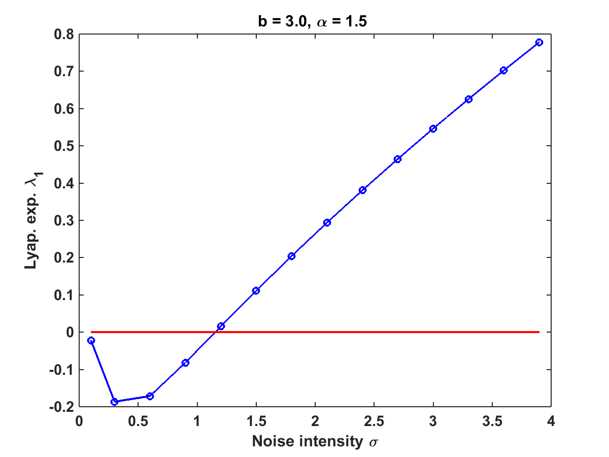
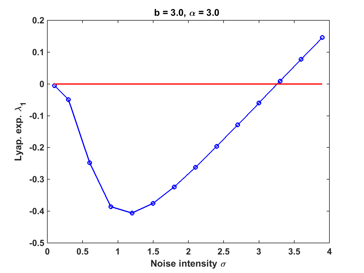
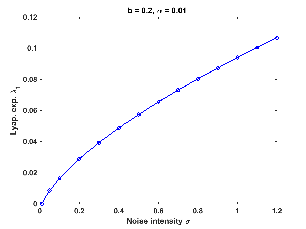
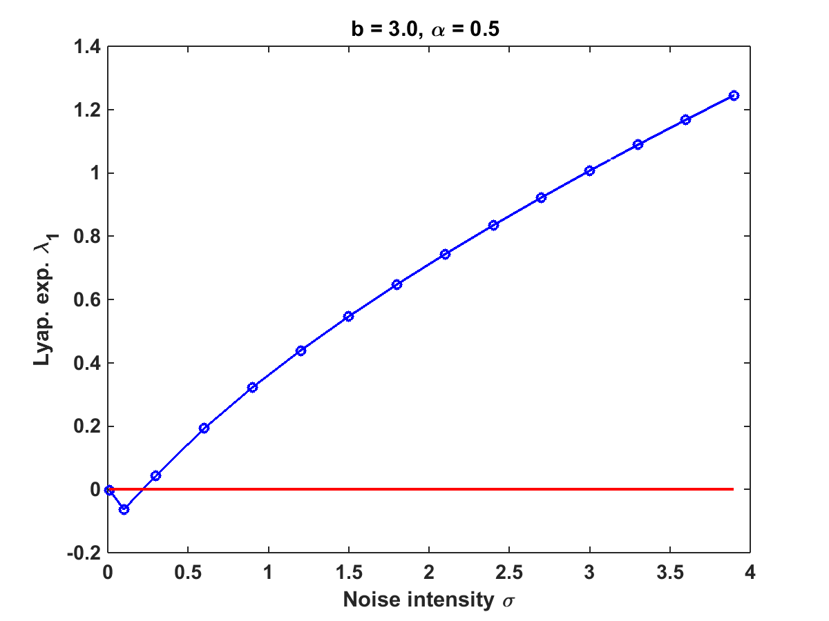
In Figure 2, we show the top Lyapunov exponent as a function of σ𝜎\sigma for fixed b𝑏b and α𝛼\alpha according to formula (2.12). We have used numerical integration up to machine precision to calculate λ1subscript𝜆1\lambda_{1}. The bifurcations of the sign of λ1subscript𝜆1\lambda_{1} at σ0(α,b)subscript𝜎0𝛼𝑏\sigma_{0}(\alpha,b) is clearly seen in Figures 2(a)-2(c). Furthermore, note that λ10subscript𝜆10\lambda_{1}\to 0 from below for σ0𝜎0\sigma\to 0. The figures illustrate that σ0(α,b)subscript𝜎0𝛼𝑏\sigma_{0}(\alpha,b) is an increasing function of α𝛼\alpha and a decreasing function of b𝑏b, or differently phrased: the larger the proportion of shear to dissipation, b/α𝑏𝛼b/\alpha, the smaller the bifurcation point σ0(α,b)subscript𝜎0𝛼𝑏\sigma_{0}(\alpha,b). In Figure 2(d), we choose small values of b𝑏b and α𝛼\alpha, but b/α𝑏𝛼b/\alpha large. We see no negative values of λ1subscript𝜆1\lambda_{1} as we would have to take values of σ𝜎\sigma too small for the numerical integration.

We have chosen the same parameter regimes as in [21], where Lin and Young investigate numerically the Lyapunov exponents of the system given by

dy=αydt+σsin(2πϑ)dWt,dϑ=(1+by)dt,d𝑦absent𝛼𝑦d𝑡𝜎2𝜋italic-ϑdsubscript𝑊𝑡ditalic-ϑabsent1𝑏𝑦d𝑡\displaystyle\begin{array}[]{r@{\;\,=\;\,}l}\mathrm{d}y&-\alpha y\mathrm{d}t+\sigma\sin(2\pi\vartheta)\circ\mathrm{d}W_{t}\,,\\ \mathrm{d}\vartheta&(1+by)\,\mathrm{d}t\,,\end{array} (3.5)

taking ϑ[0,2π]italic-ϑ02𝜋\vartheta\in[0,2\pi]. Their numerical results show exactly the same qualitative behaviour apart from a slightly different scaling due to the factor 2π2𝜋2\pi. Note that our setting contains two approximations of model (3.5). The first option is to take also one Brownian motion, i.e. m=1𝑚1m=1 in (1.3), and f1subscript𝑓1f_{1} continuous and piecewise linear with constant absolute value of the derivative almost everywhere. The accordance of the numerics for (3.5) and our results show that the simpler choice of the diffusion coefficient in our case does not change the qualitative behaviour. This is not a surprise, since we can derive formula (2.12) for λ1subscript𝜆1\lambda_{1} if we choose f𝑓f to be piecewise linear on the intervals [i4,i+14]𝑖4𝑖14[\frac{i}{4},\frac{i+1}{4}] for i=0,1,2,3𝑖0123i=0,1,2,3 with |f|superscript𝑓\left|f^{\prime}\right| constant such that it represents a linear approximation of the sine function.
Refer to caption
(a)
Refer to caption
(b)
Refer to caption
(c)
Refer to caption
(d)
Figure 2: The top Lyapunov exponent λ1subscript𝜆1\lambda_{1} as a function of σ𝜎\sigma for fixed b𝑏b and α𝛼\alpha. The dots indicate the values of λ1subscript𝜆1\lambda_{1} that were calculated according to (2.12) using numerical integration. Figures 2(a)-2(c) illustrate that σ0(α,b)subscript𝜎0𝛼𝑏\sigma_{0}(\alpha,b) increases monotonously in α𝛼\alpha. In Figure 2(d), b𝑏b and α𝛼\alpha are small, but b/α𝑏𝛼b/\alpha is large. We don’t see the transition to λ1<0subscript𝜆10\lambda_{1}<0 since we would have to take values of σ𝜎\sigma too small for the numerical integration.

The second option is given by (1.5) which adds an additional Brownian motion with the cosine function as diffusion coefficient. As we have seen, this slightly extended model does not change the qualitative behaviour and validates analytically Lin and Young’s numerical investigations for model (3.5).

Furthermore, we confirm Lin and Young’s conjecture concerning a scaling property of λ1subscript𝜆1\lambda_{1} with respect to the parameters. For model (3.5) they observed numerically that, under the transformations αkαmaps-to𝛼𝑘𝛼\alpha\mapsto k\alpha, bkbmaps-to𝑏𝑘𝑏b\mapsto kb and σkσmaps-to𝜎𝑘𝜎\sigma\mapsto\sqrt{k}\sigma, λ1subscript𝜆1\lambda_{1} transforms approximately as λ1kλ1maps-tosubscript𝜆1𝑘subscript𝜆1\lambda_{1}\mapsto k\lambda_{1}. This scaling property holds exactly for our model (1.3).

Proposition 3.3.

Consider the stochastic differential equation (1.3), where the function f𝑓f is of the form (1.6). Then the top Lyapunov exponent λ1subscript𝜆1\lambda_{1} as given by (2.12) satisfies

λ1(kα,kb,kσ)=kλ1(α,b,σ)for all k+{0}.formulae-sequencesubscript𝜆1𝑘𝛼𝑘𝑏𝑘𝜎𝑘subscript𝜆1𝛼𝑏𝜎for all 𝑘superscript0\lambda_{1}(k\alpha,kb,\sqrt{k}\sigma)=k\lambda_{1}(\alpha,b,\sigma)\quad\quad\text{for all }\,k\in\mathbb{R}^{+}\setminus\{0\}\,. (3.6)
Proof.

Recall from Proposition 2.3 that λ1subscript𝜆1\lambda_{1} can be calculated as the top Lyapunov exponent of the linear system (2.11). Then the claim follows immediately if we conduct the time change tktmaps-to𝑡𝑘𝑡t\mapsto kt in this equation. ∎

4 Summary and outlook

We have investigated systems with limit cycles on a cylinder perturbed by white noise. We were able to show a transition from negative to positive top Lyapunov exponents for fixed dissipation parameter α𝛼\alpha and big enough noise σ𝜎\sigma and/or shear b𝑏b. This implies a bifurcation of the random attractor from a random equilibrium to random strange attractor.

In the case of positive Lyapunov exponents, it remains an open problem to describe the attractor using concepts from ergodic theory, as entropy and SRB measures [19, 28], in order to have a more rigorous notion of chaos.

The results of this paper may well be relevant to shed more light on the problem of stochastic Hopf bifurcation, where numerical studies indicate a transition from negative to positive Lyapunov exponent as explained in the Introduction.

Acknowledgments

The authors would like to thank the referee for carefully reading our manuscript and for giving such constructive comments which substantially helped improving the quality of the paper, in particular strengthening the main result. We also express exceptional gratitude to Martin Hairer and Nils Berglund for suggesting a very valuable generalization of the original model. In addition, the authors thank Alexis Arnaudon, Darryl Holm, Aleksandar Mijatovic, Nikolas Nüsken, Grigorios Pavliotis and Sebastian Wieczorek for useful discussions. Maximilian Engel was supported by a Roth Scholarship from the Department of Mathematics at Imperial College London and the SFB Transregio 109 ”Discretization in Geometry and Dynamcis” sponsored by the German Research Foundation (DFG). Jeroen S.W. Lamb acknowledges the support by Nizhny Novgorod University through the grant RNF 14-41-00044, and Martin Rasmussen was supported by an EPSRC Career Acceleration Fellowship EP/I004165/1. This research has also been supported by EU Marie-Curie IRSES Brazilian-European Partnership in Dynamical Systems (FP7-PEOPLE-2012-IRSES 318999 BREUDS) and EU Marie-Skłodowska-Curie ITN Critical Transitions in Complex Systems (H2020-MSCA-2014-ITN 643073 CRITICS).

References

  • [1] A. Arnaudon, A.L. De Castro, and D.D. Holm. Noise and dissipation on coadjoint orbits. arXiv1601.02249[math.PR], 2016.
  • [2] L. Arnold. Random Dynamical Systems. Springer, Berlin, 1998.
  • [3] L. Arnold, N. Sri Namachchivaya, and K. R. Schenk-Hoppé. Toward an understanding of stochastic Hopf bifurcation: A case study. International Journal of Bifurcation and Chaos, 6(11):1947–1975, 1996.
  • [4] P.H. Baxendale. Statistical equilibrium and two-point motion for a stochastic flow of diffeomorphisms. In Spatial stochastic processes, volume 19 of Progress in Probability, pages 189–218. Birkhäuser Boston, Boston, MA, 1991.
  • [5] P.H. Baxendale. A stochastic Hopf bifurcation. Probability Theory and Related Fields, 99:581–616, 1994.
  • [6] P.H. Baxendale. Stochastic averaging and asymptotic behavior of the stochastic Duffing-van der Pol equation. Stochastic Processes and their Applications, 113:235–272, 2004.
  • [7] P.H. Baxendale and L. Goukasian. Lyapunov exponents for small perturbations of Hamiltonian systems. Annals of Probability, 30:101–134, 2002.
  • [8] M. Callaway, T.S. Doan, J.S.W. Lamb, and M. Rasmussen. The dichotomy spectrum for random dynamical systems and pitchfork bifurcations with additive noise. Annales de l’Institut Henri Poincaré, Probabilités et Statistiques, 53(4):1548–1574, 2017.
  • [9] H. Crauel and F. Flandoli. Additive noise destroys a pitchfork bifurcation. Journal of Dynamics and Differential Equations, 10(2):259–274, 1996.
  • [10] L. Deville, N. Sri Namachchivaya, and Z. Rapti. Stability of a stochastic two-dimensional non-Hamiltonian system. Journal of Applied Mathematics, 71(4):1458–1475, 2011.
  • [11] T.S. Doan, M. Engel, J.S.W. Lamb, and M. Rasmussen. Hopf bifurcation with additive noise. arXiv:1710.09649v1[math.DS], 2007.
  • [12] F. Flandoli, B. Gess, and M. Scheutzow. Synchronization by noise. Probability Theory and Related Fields, 168(3–4):511–556, 2017.
  • [13] P. Imkeller and C. Lederer. An explicit description of the Lyapunov exponents of the noisy damped harmonic oscillator. Dynamics and Stability of Systems, 14(4):385–405, 1999.
  • [14] P. Imkeller and C. Lederer. Some formulas for Lyapunov exponents and rotation numbers in two dimensions and the stability of the harmonic oscillator and the inverted pendulum. Dynamical Systems, 16(1):29–61, 2001.
  • [15] H. Keller and B Schmalfuss. Attractors for stochastic differential equations with nontrivial noise. Buletinul A.S. a R.M. Matematica, 26(1):43–54, 1998.
  • [16] P.E. Kloeden and M. Rasmussen. Nonautonomous dynamical systems, volume 176 of Mathematical Surveys and Monographs. American Mathematical Society, Providence, RI, 2011.
  • [17] J.S.W. Lamb, M. Rasmussen, and C.S. Rodrigues. Topological bifurcations of minimal invariant sets for set-valued dynamical systems. Proceedings of the American Mathematical Society, 143(9), 2015.
  • [18] Y. Le Jan. Equilibre statistique pour les produits de diffeomorphismes aleatoires independants. Annales de l’Institut Henri Poincaré, Probabilités et Statistiques, 23(1):111–120, 1987.
  • [19] F. Ledrappier and L.-S. Young. Entropy formula for random transformations. Probability Theory and Related Fields, 80:217–240, 1988.
  • [20] Z. Lian and M. Stenlund. Positive Lyapunov exponent by a random perturbation. Dynamical Systems, 27(2):239–252, 2012.
  • [21] K. K. Lin and L.-S. Young. Shear-induced chaos. Nonlinearity, 21:899–922, 2008.
  • [22] J. Newman. Necessary and sufficient conditions for stable synchronisation in random dyncamical systems. arXiv1408.5599v3[math.PR], 2015.
  • [23] J. Newman. Synchronisation of almost all trajectories of a random dynamical system. arXiv1511.08831v2[math.PR], 2015.
  • [24] W. Ott and M. Stenlund. From limit cycles to strange attractors. Communications in Mathematical Physics, 296(1):215–249, 2010.
  • [25] K. R. Schenk-Hoppé. Bifurcation scenarios of the noisy Duffing-van der Pol oscillator. Nonlinear Dynamics, 11:255–274, 1996.
  • [26] T.T. Soong. Random differential equations in science and engineering. Mathematics in Science and Engineering 103. Academic Press, New York and London, 1973.
  • [27] Q. Wang and L.-S. Young. From invariant curves to strange attractors. Communications in Mathematical Physics, 225(2):275–304, 2002.
  • [28] Q. Wang and L.-S. Young. Strange attractors in periodically-kicked limit cycles and Hopf bifurcations. Communications in Mathematical Physics, 240(3):509–529, 2003.
  • [29] S. Wieczorek. Stochastic bifurcation in noise-driven lasers and Hopf oscillators. Physical Review E, 79:1–10, 2009.
  • [30] L.-S. Young. Chaotic phenomena in three settings: large, noisy and out of equilibrium. Nonlinearity, 21:245–252, 2008.
  • [31] H. Zmarrou and A.J. Homburg. Bifurcations of stationary measures of random diffeomorphisms. Ergodic Theory and Dynamical Systems, 27(5):1651–1692, 2007.