$f$-GAN: Training Generative Neural Samplers using Variational Divergence Minimization

Abstract

Generative neural samplers are probabilistic models that implement sampling using feedforward neural networks: they take a random input vector and produce a sample from a probability distribution defined by the network weights. These models are expressive and allow efficient computation of samples and derivatives, but cannot be used for computing likelihoods or for marginalization. The generative-adversarial training method allows to train such models through the use of an auxiliary discriminative neural network. We show that the generative-adversarial approach is a special case of an existing more general variational divergence estimation approach. We show that any $f$-divergence can be used for training generative neural samplers. We discuss the benefits of various choices of divergence functions on training complexity and the quality of the obtained generative models.

1 Introduction

Probabilistic generative models describe a probability distribution over a given domain $\mathcal{X}$, for example a distribution over natural language sentences, natural images, or recorded waveforms.

Given a generative model $Q$ from a class $\mathcal{Q}$ of possible models we are generally interested in performing one or multiple of the following operations:

• Sampling. Produce a sample from $Q$. By inspecting samples or calculating a function on a set of samples we can obtain important insight into the distribution or solve decision problems.

• Estimation. Given a set of iid samples $\{x_{1},x_{2},\dots,x_{n}\}$ from an unknown true distribution $P$, find $Q\in\mathcal{Q}$ that best describes the true distribution.

• Point-wise likelihood evaluation. Given a sample $x$, evaluate the likelihood $Q(x)$.

Generative-adversarial networks (GAN) in the form proposed by [10] are an expressive class of generative models that allow exact sampling and approximate estimation. The model used in GAN is simply a feedforward neural network which receives as input a vector of random numbers, sampled, for example, from a uniform distribution. This random input is passed through each layer in the network and the final layer produces the desired output, for example, an image. Clearly, sampling from a GAN model is efficient because only one forward pass through the network is needed to produce one exact sample.

Such probabilistic feedforward neural network models were first considered in [22] and [3], here we call these models generative neural samplers. GAN is also of this type, as is the decoder model of a variational autoencoder [18].

In the original GAN paper the authors show that it is possible to estimate neural samplers by approximate minimization of the symmetric Jensen-Shannon divergence,

$$D_{\textrm{JS}}(P\|Q)=\tfrac{1}{2}D_{\textrm{KL}}(P\|\tfrac{1}{2}(P+Q))+\tfrac{1}{2}D_{\textrm{KL}}(Q\|\tfrac{1}{2}(P+Q)),$$ (1)

where $D_{KL}$ denotes the Kullback-Leibler divergence. The key technique used in the GAN training is that of introducing a second “discriminator” neural networks which is optimized simultaneously. Because $D_{\textrm{JS}}(P\|Q)$ is a proper divergence measure between distributions this implies that the true distribution $P$ can be approximated well in case there are sufficient training samples and the model class $\mathcal{Q}$ is rich enough to represent $P$.

In this work we show that the principle of GANs is more general and we can extend the variational divergence estimation framework proposed by Nguyen et al. [25] to recover the GAN training objective and generalize it to arbitrary $f$-divergences.

More concretely, we make the following contributions over the state-of-the-art:

• We derive the GAN training objectives for all $f$-divergences and provide as example additional divergence functions, including the Kullback-Leibler and Pearson divergences.

• We simplify the saddle-point optimization procedure of Goodfellow et al. [10] and provide a theoretical justification.

• We provide experimental insight into which divergence function is suitable for estimating generative neural samplers for natural images.

2 Method

We first review the divergence estimation framework of Nguyen et al. [25] which is based on $f$-divergences. We then extend this framework from divergence estimation to model estimation.

2.1 The f-divergence Family

Statistical divergences such as the well-known Kullback-Leibler divergence measure the difference between two given probability distributions. A large class of different divergences are the so called $f$-divergences [5, 21], also known as the Ali-Silvey distances [1]. Given two distributions $P$ and $Q$ that possess, respectively, an absolutely continuous density function $p$ and $q$ with respect to a base measure $\textrm{d}x$ defined on the domain $\mathcal{X}$, we define the $f$-divergence,

$$D_{f}(P\|Q)=\int_{\mathcal{X}}q(x)f\left(\frac{p(x)}{q(x)}\right)\,\textrm{d}x,$$ (2)

where the generator function $f:\mathbb{R}_{+}\to\mathbb{R}$ is a convex, lower-semicontinuous function satisfying $f(1)=0$. Different choices of $f$ recover popular divergences as special cases in (2). We illustrate common choices in Table 5. See supplementary material for more divergences and plots.

2.2 Variational Estimation of $f$-divergences

Nguyen et al. [25] derive a general variational method to estimate $f$-divergences given only samples from $P$ and $Q$. We will extend their method from merely estimating a divergence for a fixed model to estimating model parameters. We call this new method variational divergence minimization (VDM) and show that the generative-adversarial training is a special case of this more general VDM framework.

For completeness, we first provide a self-contained derivation of Nguyen et al’s divergence estimation procedure. Every convex, lower-semicontinuous function $f$ has a convex conjugate function $f^{*}$, also known as Fenchel conjugate [14]. This function is defined as

$$f^{*}(t)=\sup_{u\in\textrm{dom}_{f}}\left\{ut-f(u)\right\}.$$ (3)

The function $f^{*}$ is again convex and lower-semicontinuous and the pair $(f,f^{*})$ is dual to another in the sense that $f^{**}=f$. Therefore, we can also represent $f$ as $f(u)=\sup_{t\in\textrm{dom}_{f^{*}}}\left\{tu-f^{*}(t)\right\}$. Nguyen et al. leverage the above variational representation of $f$ in the definition of the $f$-divergence to obtain a lower bound on the divergence,

$$D_{f}(P\|Q) =\textstyle\bigintsss_{\mathcal{X}}q(x)\sup\limits_{t\in\textrm{dom}_{f^{*}}}\left\{t\frac{p(x)}{q(x)}-f^{*}(t)\right\}\,\textrm{d}x$$

$$\geq\textstyle\sup_{T\in\mathcal{T}}\left(\bigintsss_{\mathcal{X}}p(x)\,T(x)\,\textrm{d}x-\textstyle\bigintsss_{\mathcal{X}}q(x)\,f^{*}(T(x))\,\textrm{d}x\right)$$

$$=\sup_{T\in\mathcal{T}}\left(\mathbb{E}_{x\sim P}\left[T(x)\right]-\mathbb{E}_{x\sim Q}\left[f^{*}(T(x))\right]\right),$$ (4)

where $\mathcal{T}$ is an arbitrary class of functions $T:\mathcal{X}\to\mathbb{R}$. The above derivation yields a lower bound for two reasons: first, because of Jensen’s inequality when swapping the integration and supremum operations. Second, the class of functions $\mathcal{T}$ may contain only a subset of all possible functions.

By taking the variation of the lower bound in (4) w.r.t. $T$, we find that under mild conditions on $f$ [25], the bound is tight for

$$T^{\ast}(x)=f^{\prime}\left(\frac{p(x)}{q(x)}\right),$$ (5)

where $f^{\prime}$ denotes the first order derivative of $f$. This condition can serve as a guiding principle for choosing $f$ and designing the class of functions $\mathcal{T}$. For example, the popular reverse Kullback-Leibler divergence corresponds to $f(u)=-\log(u)$ resulting in $T^{\ast}(x)=-q(x)/p(x)$, see Table 5.

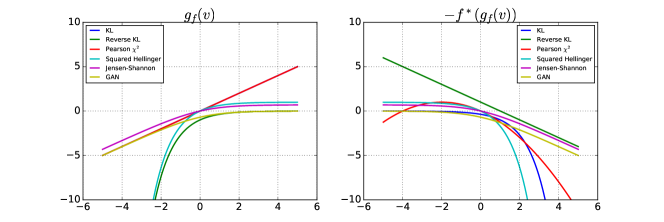
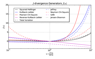
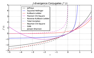
We list common $f$-divergences in Table 5 and provide their Fenchel conjugates $f^{*}$ and the domains $\textrm{dom}_{f^{*}}$ in Table 6. We provide plots of the generator functions and their conjugates in the supplementary materials.

Name	$D_{f}(P\|Q)$	Generator $f(u)$	$T^{\ast}(x)$
Kullback-Leibler	$\int p(x)\log\frac{p(x)}{q(x)}\,\textrm{d}x$	$u\log u$	$1+\log\frac{p(x)}{q(x)}$
Reverse KL	$\int q(x)\log\frac{q(x)}{p(x)}\,\textrm{d}x$	$-\log u$	$-\frac{q(x)}{p(x)}$
Pearson $\chi^{2}$	$\int\frac{(q(x)-p(x))^{2}}{p(x)}\,\textrm{d}x$	$(u-1)^{2}$	$2(\frac{p(x)}{q(x)}-1)$
Squared Hellinger	$\int\left(\sqrt{p(x)}-\sqrt{q(x)}\right)^{2}\,\textrm{d}x$	$\left(\sqrt{u}-1\right)^{2}$	$(\sqrt{\frac{p(x)}{q(x)}}-1)\cdot\sqrt{\frac{q(x)}{p(x)}}$
Jensen-Shannon	$\frac{1}{2}\int p(x)\log\frac{2p(x)}{p(x)+q(x)}+q(x)\log\frac{2q(x)}{p(x)+q(x)}\,\textrm{d}x$	$-(u+1)\log\frac{1+u}{2}+u\log u$	$\log\frac{2p(x)}{p(x)+q(x)}$
GAN	$\int p(x)\log\frac{2p(x)}{p(x)+q(x)}+q(x)\log\frac{2q(x)}{p(x)+q(x)}\,\textrm{d}x-\log(4)$	$u\log u-(u+1)\log(u+1)$	$\log\frac{p(x)}{p(x)+q(x)}$

Table 1: List of $f$-divergences $D_{f}(P\|Q)$ together with generator functions. Part of the list of divergences and their generators is based on [26]. For all divergences we have $f:\textrm{dom}_{f}\to\mathbb{R}\cup\{+\infty\}$, where $f$ is convex and lower-semicontinuous. Also we have $f(1)=0$ which ensures that $D_{f}(P\|P)=0$ for any distribution $P$. As shown by [10] GAN is related to the Jensen-Shannon divergence through $D_{\textrm{GAN}}=2D_{\textrm{JS}}-\log(4)$.

2.3 Variational Divergence Minimization (VDM)

We now use the variational lower bound (4) on the $f$-divergence $D_{f}(P\|Q)$ in order to estimate a generative model $Q$ given a true distribution $P$.

To this end, we follow the generative-adversarial approach [10] and use two neural networks, $Q$ and $T$. $Q$ is our generative model, taking as input a random vector and outputting a sample of interest. We parametrize $Q$ through a vector $\theta$ and write $Q_{\theta}$. $T$ is our variational function, taking as input a sample and returning a scalar. We parametrize $T$ using a vector $\omega$ and write $T_{\omega}$.

We can learn a generative model $Q_{\theta}$ by finding a saddle-point of the following $f$-GAN objective function, where we minimize with respect to $\theta$ and maximize with respect to $\omega$,

$$F(\theta,\omega)=\mathbb{E}_{x\sim P}\left[T_{\omega}(x)\right]-\mathbb{E}_{x\sim Q_{\theta}}\left[f^{*}(T_{\omega}(x))\right].$$ (6)

To optimize (6) on a given finite training data set, we approximate the expectations using minibatch samples. To approximate $\mathbb{E}_{x\sim P}[\cdot]$ we sample $B$ instances without replacement from the training set. To approximate $\mathbb{E}_{x\sim Q_{\theta}}[\cdot]$ we sample $B$ instances from the current generative model $Q_{\theta}$.

2.4 Representation for the Variational Function

To apply the variational objective (6) for different $f$-divergences, we need to respect the domain $\textrm{dom}_{f^{*}}$ of the conjugate functions $f^{*}$. To this end, we assume that variational function $T_{\omega}$ is represented in the form $T_{\omega}(x)=g_{f}(V_{\omega}(x))$ and rewrite the saddle objective (6) as follows:

$$F(\theta,\omega)=\mathbb{E}_{x\sim P}\left[g_{f}(V_{\omega}(x))\right]+\mathbb{E}_{x\sim Q_{\theta}}\left[-f^{*}(g_{f}(V_{\omega}(x)))\right],$$ (7)

where $V_{\omega}:\mathcal{X}\to\mathbb{R}$ without any range constraints on the output, and $g_{f}:\mathbb{R}\to\textrm{dom}_{f^{*}}$ is an output activation function specific to the $f$-divergence used. In Table 6 we propose suitable output activation functions for the various conjugate functions $f^{*}$ and their domains. Although the choice of $g_{f}$ is somewhat arbitrary, we choose all of them to be monotone increasing functions so that a large output $V_{\omega}(x)$ corresponds to the belief of the variational function that the sample $x$ comes from the data distribution $P$ as in the GAN case; see Figure 1. It is also instructive to look at the second term $-f^{\ast}(g_{f}(v))$ in the saddle objective (7). This term is typically (except for the Pearson $\chi^{2}$ divergence) a decreasing function of the output $V_{\omega}(x)$ favoring variational functions that output negative numbers for samples from the generator.

Name	Output activation $g_{f}$	$\textrm{dom}_{f^{*}}$	Conjugate $f^{*}(t)$	$f^{\prime}(1)$
Kullback-Leibler (KL)	$v$	$\mathbb{R}$	$\exp(t-1)$	$1$
Reverse KL	$-\exp(-v)$	$\mathbb{R}_{-}$	$-1-\log(-t)$	$-1$
Pearson $\chi^{2}$	$v$	$\mathbb{R}$	$\frac{1}{4}t^{2}+t$	$0$
Squared Hellinger	$1-\exp(-v)$	$t<1$	$\frac{t}{1-t}$	$0$
Jensen-Shannon	$\log(2)-\log(1+\exp(-v))$	$t<\log(2)$	$-\log(2-\exp(t))$	$0$
GAN	$-\log(1+\exp(-v))$	$\mathbb{R}_{-}$	$-\log(1-\exp(t))$	$-\log(2)$

Table 2: Recommended final layer activation functions and critical variational function level defined by $f^{\prime}(1)$. The critical value $f^{\prime}(1)$ can be interpreted as a classification threshold applied to $T(x)$ to distinguish between true and generated samples.

We can see the GAN objective,

$$F(\theta,\omega)=\mathbb{E}_{x\sim P}\left[\log D_{\omega}(x)\right]+\mathbb{E}_{x\sim Q_{\theta}}\left[\log(1-D_{\omega}(x))\right],$$ (8)

as a special instance of (7) by identifying each terms in the expectations of (7) and (8). In particular, choosing the last nonlinearity in the discriminator as the sigmoid $D_{\omega}(x)=1/(1+e^{-V_{\omega}(x)})$, corresponds to output activation function is $g_{f}(v)=-\log(1+e^{-v})$; see Table 6.

Figure 1: The two terms in the saddle objective (7) are plotted as a function of the variational function $V_{\omega}(x)$.

2.5 Example: Univariate Mixture of Gaussians

	KL	KL-rev	JS	Jeffrey	Pearson
$D_{f}(P\rvert\lvert Q_{{\theta}^{\ast}})$	0.2831	0.2480	0.1280	0.5705	0.6457
$F(\hat{\omega},\hat{\theta})$	0.2801	0.2415	0.1226	0.5151	0.6379
$\mu^{\ast}$	1.0100	1.5782	1.3070	1.3218	0.5737
$\hat{\mu}$	1.0335	1.5624	1.2854	1.2295	0.6157
$\sigma^{\ast}$	1.8308	1.6319	1.7542	1.7034	1.9274
$\hat{\sigma}$	1.8236	1.6403	1.7659	1.8087	1.9031

train $\backslash$ test	KL	KL-rev	JS	Jeffrey	Pearson
KL	0.2808	0.3423	0.1314	0.5447	0.7345
KL-rev	0.3518	0.2414	0.1228	0.5794	1.3974
JS	0.2871	0.2760	0.1210	0.5260	0.92160
Jeffrey	0.2869	0.2975	0.1247	0.5236	0.8849
Pearson	0.2970	0.5466	0.1665	0.7085	0.648

Table 3: Gaussian approximation of a mixture of Gaussians. Left: optimal objectives, and the learned mean and the standard deviation: $\hat{\theta}=(\hat{\mu},\hat{\sigma})$ (learned) and $\theta^{\ast}=(\mu^{\ast},\sigma^{\ast})$ (best fit). Right: objective values to the true distribution for each trained model. For each divergence, the lowest objective function value is achieved by the model that was trained for this divergence.

To demonstrate the properties of the different $f$-divergences and to validate the variational divergence estimation framework we perform an experiment similar to the one of [24].

Setup. We approximate a mixture of Gaussians by learning a Gaussian distribution. We represent our model $Q_{\theta}$ using a linear function which receives a random $z\sim\mathcal{N}(0,1)$ and outputs $G_{\theta}(z)=\mu+\sigma z$, where $\theta=(\mu,\sigma)$ are the two scalar parameters to be learned. For the variational function $T_{\omega}$ we use a neural network with two hidden layers having $64$ units each and tanh activations. We optimise the objective $F(\omega,\theta)$ by using the single-step gradient method presented in Section 3. In each step we sample batches of size $1024$ each for both $p(x)$ and $p(z)$ and we use a step-size of $\eta=0.01$ for updating both $\omega$ and $\theta$. We compare the results to the best fit provided by the exact optimization of $D_{f}(P\|Q_{\theta})$ w.r.t. $\theta$, which is feasible in this case by solving the required integrals in (2) numerically. We use $(\hat{\omega},\hat{\theta})$ (learned) and $\theta^{\ast}$ (best fit) to distinguish the parameters sets used in these two approaches.

Results. The left side of Table 3 shows the optimal divergence and objective values $D_{f}(P\rvert\lvert Q_{{\theta}^{\ast}})$ and $F(\hat{\omega},\hat{\theta})$ as well as the resulting means and standard deviations. Note that the results are in line with the lower bound property, that is, we have $D_{f}(P\rvert\lvert Q_{{\theta}^{\ast}})\geq F(\hat{\omega},\hat{\theta})$. There is a good correspondence between the gap in objectives and the difference between the fitted means and standard deviations. The right side of Table 3 shows the results of the following experiment: (1) we train $T_{\omega}$ and $Q_{\theta}$ using a particular divergence, then (2) we estimate the divergence and re-train $T_{\omega}$ while keeping $Q_{\theta}$ fixed. As expected, $Q_{\theta}$ performs best on the divergence it was trained with. Further details showing detailed plots of the fitted Gaussians and the optimal variational functions are presented in the supplementary materials.

In summary, the above results demonstrate that when the generative model is misspecified and does not contain the true distribution, the divergence function used for estimation has a strong influence on which model is learned.

3 Algorithms for Variational Divergence Minimization (VDM)

We now discuss numerical methods to find saddle points of the objective (6). To this end, we distinguish two methods; first, the alternating method originally proposed by Goodfellow et al. [10], and second, a more direct single-step optimization procedure.

In our variational framework, the alternating gradient method can be described as a double-loop method; the internal loop tightens the lower bound on the divergence, whereas the outer loop improves the generator model. While the motivation for this method is plausible, in practice the choice taking a single step in the inner loop is popular. Goodfellow et al. [10] provide a local convergence guarantee.

3.1 Single-Step Gradient Method

Motivated by the success of the alternating gradient method with a single inner step, we propose a simpler algorithm shown in Algorithm 1. The algorithm differs from the original one in that there is no inner loop and the gradients with respect to $\omega$ and $\theta$ are computed in a single back-propagation.

Algorithm 1 Single-Step Gradient Method

1:function SingleStepGradientIteration($P,\theta^{t},\omega^{t},B,\eta$)

2:     Sample $X_{P}=\{x_{1},\ldots,x_{B}\}$ and $X_{Q}=\{x^{\prime}_{1},\ldots,x^{\prime}_{B}\}$, from $P$ and $Q_{\theta^{t}}$, respectively.

3:     Update: $\omega^{t+1}=\omega^{t}+\eta\,\nabla_{\omega}F(\theta^{t},\omega^{t})$.

4:     Update: $\theta^{t+1}=\theta^{t}-\eta\,\nabla_{\theta}F(\theta^{t},\omega^{t})$.

5:end function

Analysis.

Here we show that Algorithm 1 geometrically converges to a saddle point $(\theta^{\ast},\omega^{\ast})$ if there is a neighborhood around the saddle point in which $F$ is strongly convex in $\theta$ and strongly concave in $\omega$. These conditions are similar to the assumptions made in [10] and can be formalized as follows:

$$\nabla_{\theta}F(\theta^{\ast},\omega^{\ast})=0,\quad\nabla_{\omega}F(\theta^{\ast},\omega^{\ast})=0,\quad\nabla_{\theta}^{2}F(\theta,\omega)\succeq\delta I,\quad\nabla_{\omega}^{2}F(\theta,\omega)\preceq-\delta I.$$ (9)

These assumptions are necessary except for the “strong” part in order to define the type of saddle points that are valid solutions of our variational framework. Note that although there could be many saddle points that arise from the structure of deep networks [6], they do not qualify as the solution of our variational framework under these assumptions.

For convenience, let’s define $\pi^{t}=(\theta^{t},\omega^{t})$. Now the convergence of Algorithm 1 can be stated as follows (the proof is given in the supplementary material):

Theorem 1.

Suppose that there is a saddle point $\pi^{\ast}=(\theta^{\ast},\omega^{\ast})$ with a neighborhood that satisfies conditions (9). Moreover, we define $J(\pi)=\frac{1}{2}\|\nabla F(\pi)\|_{2}^{2}$ and assume that in the above neighborhood, $F$ is sufficiently smooth so that there is a constant $L>0$ such that $\|\nabla J(\pi^{\prime})-\nabla J(\pi)\|_{2}\leq L\|\pi^{\prime}-\pi\|_{2}$ for any $\pi,\pi^{\prime}$ in the neighborhood of $\pi^{\ast}$. Then using the step-size $\eta=\delta/L$ in Algorithm 1, we have

$$J(\pi^{t})\leq\left(1-\frac{\delta^{2}}{2L}\right)^{t}J(\pi^{0})$$

That is, the squared norm of the gradient $\nabla F(\pi)$ decreases geometrically.

3.2 Practical Considerations

Here we discuss principled extensions of the heuristic proposed in [10] and real/fake statistics discussed by Larsen and Sønderby. Furthermore we discuss practical advice that slightly deviate from the principled viewpoint.

Goodfellow et al. [10] noticed that training GAN can be significantly sped up by maximizing $\mathbb{E}_{x\sim Q_{\theta}}\left[\log D_{\omega}(x)\right]$ instead of minimizing $\mathbb{E}_{x\sim Q_{\theta}}\left[\log\left(1-D_{\omega}(x)\right)\right]$ for updating the generator. In the more general $f$-GAN Algorithm (1) this means that we replace line 4 with the update

$$\theta^{t+1}=\theta^{t}+\eta\,\nabla_{\theta}\mathbb{E}_{x\sim Q_{\theta^{t}}}[g_{f}(V_{\omega^{t}}(x))],$$ (10)

thereby maximizing the generator output. This is not only intuitively correct but we can show that the stationary point is preserved by this change using the same argument as in [10]; we found this useful also for other divergences.

Larsen and Sønderby recommended monitoring real and fake statistics, which are defined as the true positive and true negative rates of the variational function viewing it as a binary classifier. Since our output activation $g_{f}$ are all monotone, we can derive similar statistics for any $f$-divergence by only changing the decision threshold. Due to the link between the density ratio and the variational function (5), the threshold lies at $f^{\prime}(1)$ (see Table 6). That is, we can interpret the output of the variational function as classifying the input $x$ as a true sample if the variational function $T_{\omega}(x)$ is larger than $f^{\prime}(1)$, and classifying it as a sample from the generator otherwise.

We found Adam [17] and gradient clipping to be useful especially in the large scale experiment on the LSUN dataset.

4 Experiments

We now train generative neural samplers based on VDM on the MNIST and LSUN datasets.

MNIST Digits.

We use the MNIST training data set (60,000 samples, 28-by-28 pixel images) to train the generator and variational function model proposed in [10] for various $f$-divergences. With $z\sim\textrm{Uniform}_{100}(-1,1)$ as input, the generator model has two linear layers each followed by batch normalization and ReLU activation and a final linear layer followed by the sigmoid function. The variational function $V_{\omega}(x)$ has three linear layers with exponential linear unit [4] in between. The final activation is specific to each divergence and listed in Table 6. As in [27] we use Adam with a learning rate of $\alpha=0.0002$ and update weight $\beta=0.5$. We use a batchsize of 4096, sampled from the training set without replacement, and train each model for one hour. We also compare against variational autoencoders [18] with 20 latent dimensions.

Results and Discussion. We evaluate the performance using the kernel density estimation (Parzen window) approach used in [10]. To this end, we sample 16k images from the model and estimate a Parzen window estimator using an isotropic Gaussian kernel bandwidth using three fold cross validation. The final density model is used to evaluate the average log-likelihood on the MNIST test set (10k samples). We show the results in Table 4, and some samples from our models in Figure 2.

The use of the KDE approach to log-likelihood estimation has known deficiencies [31]. In particular, for the dimensionality used in MNIST ($d=784$) the number of model samples required to obtain accurate log-likelihood estimates is infeasibly large. We found a large variability (up to 50 nats) between multiple repetitions. As such the results are not entirely conclusive. We also trained the same KDE estimator on the MNIST training set, achieving a significantly higher holdout likelihood. However, it is reassuring to see that the model trained for the Kullback-Leibler divergence indeed achieves a high holdout likelihood compared to the GAN model.

Training divergence	KDE $\langle LL\rangle$ (nats)	$\pm$ SEM
Kullback-Leibler	416	5.62
Reverse Kullback-Leibler	319	8.36
Pearson $\chi^{2}$	429	5.53
Neyman $\chi^{2}$	300	8.33
Squared Hellinger	-708	18.1
Jeffrey	-2101	29.9
Jensen-Shannon	367	8.19
GAN	305	8.97
Variational Autoencoder [18]	445	5.36
KDE MNIST train (60k)	502	5.99

Table 4: Kernel Density Estimation evaluation on the MNIST test data set. Each KDE model is build from 16,384 samples from the learned generative model. We report the mean log-likelihood on the MNIST test set ($n=10,000$) and the standard error of the mean. The KDE MNIST result is using 60,000 MNIST training images to fit a single KDE model.

Figure 2: MNIST model samples trained using KL, reverse KL, Hellinger, Jensen from top to bottom.

LSUN Natural Images.

Through the DCGAN work [27] the generative-adversarial approach has shown real promise in generating natural looking images. Here we use the same architecture as as in [27] and replace the GAN objective with our more general $f$-GAN objective.

We use the large scale LSUN database [34] of natural images of different categories. To illustrate the different behaviors of different divergences we train the same model on the classroom category of images, containing 168,103 images of classroom environments, rescaled and center-cropped to 96-by-96 pixels.

Setup. We use the generator architecture and training settings proposed in DCGAN [27]. The model receives $z\in{\rm Uniform}_{d_{\rm rand}}(-1,1)$ and feeds it through one linear layer and three deconvolution layers with batch normalization and ReLU activation in between. The variational function is the same as the discriminator architecture in [27] and follows the structure of a convolutional neural network with batch normalization, exponential linear units [4] and one final linear layer.

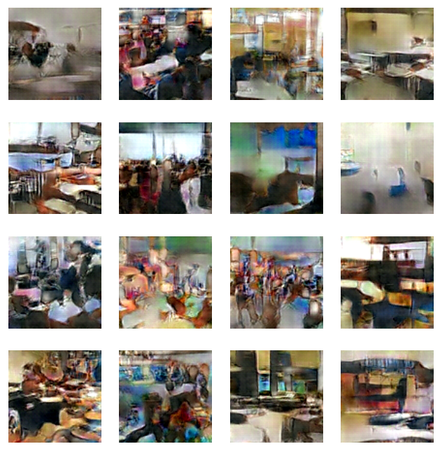
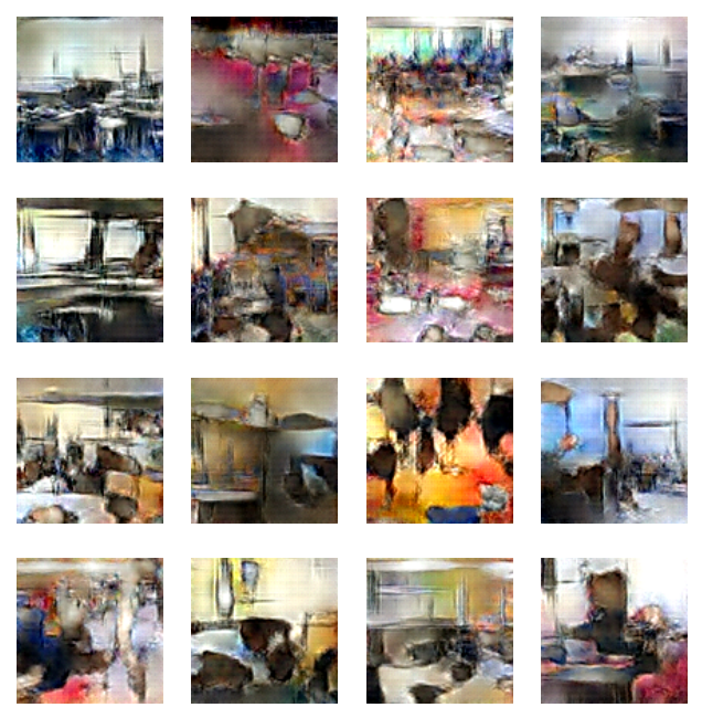
Results. Figure 3 shows 16 random samples from neural samplers trained using GAN, KL, and squared Hellinger divergences. All three divergences produce equally realistic samples. Note that the difference in the learned distribution $Q_{\theta}$ arise only when the generator model is not rich enough.

(a) GAN

(b) KL

(c) Squared Hellinger

Figure 3: Samples from three different divergences.

5 Related Work

We now discuss how our approach relates to existing work. Building generative models of real world distributions is a fundamental goal of machine learning and much related work exists. We only discuss work that applies to neural network models.

Mixture density networks [2] are neural networks which directly regress the parameters of a finite parametric mixture model. When combined with a recurrent neural network this yields impressive generative models of handwritten text [11].

NADE [19] and RNADE [33] perform a factorization of the output using a predefined and somewhat arbitrary ordering of output dimensions. The resulting model samples one variable at a time conditioning on the entire history of past variables. These models provide tractable likelihood evaluations and compelling results but it is unclear how to select the factorization order in many applications .

Diffusion probabilistic models [29] define a target distribution as a result of a learned diffusion process which starts at a trivial known distribution. The learned model provides exact samples and approximate log-likelihood evaluations.

Noise contrastive estimation (NCE) [13] is a method that estimates the parameters of unnormalized probabilistic models by performing non-linear logistic regression to discriminate the data from artificially generated noise. NCE can be viewed as a special case of GAN where the discriminator is constrained to a specific form that depends on the model (logistic regression classifier) and the generator (kept fixed) is providing the artificially generated noise (see supplementary material).

The generative neural sampler models of [22] and [3] did not provide satisfactory learning methods; [22] used importance sampling and [3] expectation maximization. The main difference to GAN and to our work really is in the learning objective, which is effective and computationally inexpensive.

Variational auto-encoders (VAE) [18, 28] are pairs of probabilistic encoder and decoder models which map a sample to a latent representation and back, trained using a variational Bayesian learning objective. The advantage of VAEs is in the encoder model which allows efficient inference from observation to latent representation and overall they are a compelling alternative to $f$-GANs and recent work has studied combinations of the two approaches [23]

As an alternative to the GAN training objective the work [20] and independently [7] considered the use of the kernel maximum mean discrepancy (MMD) [12, 9] as a training objective for probabilistic models. This objective is simpler to train compared to GAN models because there is no explicitly represented variational function. However, it requires the choice of a kernel function and the reported results so far seem slightly inferior compared to GAN. MMD is a particular instance of a larger class of probability metrics [30] which all take the form $D(P,Q)=\sup_{T\in\mathcal{T}}\left|\mathbb{E}_{x\sim P}[T(x)]-\mathbb{E}_{x\sim Q}[T(x)]\right|$, where the function class $\mathcal{T}$ is chosen in a manner specific to the divergence. Beyond MMD other popular metrics of this form are the total variation metric (also an $f$-divergence), the Wasserstein distance, and the Kolmogorov distance.

In [16] a generalisation of the GAN objective is proposed by using an alternative Jensen-Shannon divergence that mimics an interpolation between the KL and the reverse KL divergence and has Jensen-Shannon as its mid-point. It can be shown that with $\pi$ close to $0$ and $1$ it leads to a behavior similar the objectives resulting from the KL and reverse KL divergences (see supplementary material).

6 Discussion

Generative neural samplers offer a powerful way to represent complex distributions without limiting factorizing assumptions. However, while the purely generative neural samplers as used in this paper are interesting their use is limited because after training they cannot be conditioned on observed data and thus are unable to provide inferences.

We believe that in the future the true benefits of neural samplers for representing uncertainty will be found in discriminative models and our presented methods extend readily to this case by providing additional inputs to both the generator and variational function as in the conditional GAN model [8].

Acknowledgements. We thank Ferenc Huszár for discussions on the generative-adversarial approach.

Supplementary Materials

Appendix A Introduction

We provide additional material to support the content presented in the paper. The text is structured as follows. In Section B we present an extended list of f-divergences, corresponding generator functions and their convex conjugates. In Section C we provide the proof of Theorem 2 from Section 3. In Section D we discuss the differences between current (to our knowledge) GAN optimisation algorithms. Section E provides a proof of concept of our approach by fitting a Gaussian to a mixture of Gaussians using various divergence measures. Finally, in Section F we present the details of the network architectures used in Section 4 of the main text.

Appendix B $f$-divergences and Generator-Conjugate Pairs

In Table 5 we show an extended list of f-divergences $D_{f}(P\|Q)$ together with their generators $f(u)$ and the corresponding optimal variational functions $T^{\ast}(x)$. For all divergences we have $f:\textrm{dom}_{f}\to\mathbb{R}\cup\{+\infty\}$, where $f$ is convex and lower-semicontinuous. Also we have $f(1)=0$ which ensures that $D_{f}(P\|P)=0$ for any distribution $P$. As shown by [10] GAN is related to the Jensen-Shannon divergence through $D_{\textrm{GAN}}=2D_{\textrm{JS}}-\log(4)$. The GAN generator function $f$ does not satisfy $f(1)=0$ hence $D_{\textrm{GAN}}(P\|P)\neq 0$.

Table 6 lists the convex conjugate functions $f^{\ast}(t)$ of the generator functions $f(u)$ in Table 5, their domains, as well as the activation functions $g_{f}$ we use in the last layers of the generator networks to obtain a correct mapping of the network outputs into the domains of the conjugate functions.

The panels of Figure 4 show the generator functions and the corresponding convex conjugate functions for a variety of f-divergences.

Name	$D_{f}(P\|Q)$	Generator $f(u)$	$T^{\ast}(x)$
Total variation	$\frac{1}{2}\int|p(x)-q(x)|\,\textrm{d}x$	$\frac{1}{2}|u-1|$	$\frac{1}{2}{\rm sign}(\frac{p(x)}{q(x)}-1)$
Kullback-Leibler	$\int p(x)\log\frac{p(x)}{q(x)}\,\textrm{d}x$	$u\log u$	$1+\log\frac{p(x)}{q(x)}$
Reverse Kullback-Leibler	$\int q(x)\log\frac{q(x)}{p(x)}\,\textrm{d}x$	$-\log u$	$-\frac{q(x)}{p(x)}$
Pearson $\chi^{2}$	$\int\frac{(q(x)-p(x))^{2}}{p(x)}\,\textrm{d}x$	$(u-1)^{2}$	$2(\frac{p(x)}{q(x)}-1)$
Neyman $\chi^{2}$	$\int\frac{(p(x)-q(x))^{2}}{q(x)}\,\textrm{d}x$	$\frac{(1-u)^{2}}{u}$	$1-\big{[}\frac{q(x)}{p(x)}\big{]}^{2}$
Squared Hellinger	$\int\left(\sqrt{p(x)}-\sqrt{q(x)}\right)^{2}\,\textrm{d}x$	$\left(\sqrt{u}-1\right)^{2}$	$(\sqrt{\frac{p(x)}{q(x)}}-1)\cdot\sqrt{\frac{q(x)}{p(x)}}$
Jeffrey	$\int\left(p(x)-q(x)\right)\log\left(\frac{p(x)}{q(x)}\right)\,\textrm{d}x$	$(u-1)\log u$	$1+\log\frac{p(x)}{q(x)}-\frac{q(x)}{p(x)}$
Jensen-Shannon	$\frac{1}{2}\int p(x)\log\frac{2p(x)}{p(x)+q(x)}+q(x)\log\frac{2q(x)}{p(x)+q(x)}\,\textrm{d}x$	$-(u+1)\log\frac{1+u}{2}+u\log u$	$\log\frac{2p(x)}{p(x)+q(x)}$
Jensen-Shannon-weighted	$\int p(x)\pi\log\frac{p(x)}{\pi p(x)+(1-\pi)q(x)}+(1-\pi)q(x)\log\frac{q(x)}{\pi p(x)+(1-\pi)q(x)}\,\textrm{d}x$	$\pi u\log u-(1-\pi+\pi u)\log(1-\pi+\pi u)$	$\pi\log\frac{p(x)}{(1-\pi)q(x)+\pi p(x)}$
GAN	$\int p(x)\log\frac{2p(x)}{p(x)+q(x)}+q(x)\log\frac{2q(x)}{p(x)+q(x)}\,\textrm{d}x-\log(4)$	$u\log u-(u+1)\log(u+1)$	$\log\frac{p(x)}{p(x)+q(x)}$
$\alpha$-divergence ($\alpha\notin\{0,1\}$)	$\frac{1}{\alpha(\alpha-1)}\int\left(p(x)\left[\left(\frac{q(x)}{p(x)}\right)^{\alpha}-1\right]-\alpha(q(x)-p(x))\right)\,\textrm{d}x$	$\frac{1}{\alpha(\alpha-1)}\left(u^{\alpha}-1-\alpha(u-1)\right)$	$\frac{1}{\alpha-1}\Big{[}\big{[}\frac{p(x)}{q(x)}\big{]}^{\alpha-1}-1\Big{]}$

Table 5: List of $f$-divergences $D_{f}(P\|Q)$ together with generator functions and the optimal variational functions.

Name	Output activation $g_{f}$	$\textrm{dom}_{f^{*}}$	Conjugate $f^{*}(t)$	$f^{\prime}(1)$
Total variation	$\frac{1}{2}\tanh(v)$	$-\frac{1}{2}\leq t\leq\frac{1}{2}$	$t$	$0$
Kullback-Leibler (KL)	$v$	$\mathbb{R}$	$\exp(t-1)$	$1$
Reverse KL	$-\exp(v)$	$\mathbb{R}_{-}$	$-1-\log(-t)$	$-1$
Pearson $\chi^{2}$	$v$	$\mathbb{R}$	$\frac{1}{4}t^{2}+t$	$0$
Neyman $\chi^{2}$	$1-\exp(v)$	$t<1$	$2-2\sqrt{1-t}$	$0$
Squared Hellinger	$1-\exp(v)$	$t<1$	$\frac{t}{1-t}$	$0$
Jeffrey	$v$	$\mathbb{R}$	$W(e^{1-t})+\frac{1}{W(e^{1-t})}+t-2$	$0$
Jensen-Shannon	$\log(2)-\log(1+\exp(-v))$	$t<\log(2)$	$-\log(2-\exp(t))$	$0$
Jensen-Shannon-weighted	$-\pi\log\pi-\log(1+\exp(-v))$	$t<-\pi\log\pi$	$(1-\pi)\log\frac{1-\pi}{1-\pi e^{t/\pi}}$	$0$
GAN	$-\log(1+\exp(-v))$	$\mathbb{R}_{-}$	$-\log(1-\exp(t))$	$-\log(2)$
$\alpha$-div. ($\alpha<1$, $\alpha\neq 0$)	$\frac{1}{1-\alpha}-\log(1+\exp(-v))$	$t<\frac{1}{1-\alpha}$	$\frac{1}{\alpha}(t(\alpha-1)+1)^{\frac{\alpha}{\alpha-1}}-\frac{1}{\alpha}$	$0$
$\alpha$-div. ($\alpha>1$)	$v$	$\mathbb{R}$	$\frac{1}{\alpha}(t(\alpha-1)+1)^{\frac{\alpha}{\alpha-1}}-\frac{1}{\alpha}$	$0$

Table 6: Recommended final layer activation functions and critical variational function level defined by $f^{\prime}(1)$. The objective function for training a generative neural sampler $Q_{\theta}$ given a true distribution $P$ and an auxiliary variational function $T$ is $\min_{\theta}\max_{\omega}F(\theta,\omega)=\mathbb{E}_{x\sim P}[T_{\omega}(x)]-\mathbb{E}_{x\sim Q_{\theta}}[f^{*}(T_{\omega}(x))]$. For any sample $x$ the variational function produces a scalar $v(x)\in\mathbb{R}$. The output activation provides a differentiable map $g_{f}:\mathbb{R}\to\textrm{dom}_{f^{*}}$, defining $T(x)=g_{f}(v(x))$. The critical value $f^{\prime}(1)$ can be interpreted as a classification threshold applied to $T(x)$ to distinguish between true and generated samples. $W$ is the Lambert-$W$ product log function.

Figure 4: Generator-conjugate $(f,f^{*})$ pairs in the variational framework of Nguyen et al. [25]. Left: generator functions $f$ used in the $f$-divergence $D_{f}(P\|Q)=\int_{\mathcal{X}}q(x)f\left(\frac{p(x)}{q(x)}\right)\,\textrm{d}x$. Right: conjugate functions $f^{*}$ in the variational divergence lower bound $D_{f}(P\|Q)\geq\sup_{T\in\mathcal{T}}\int_{\mathcal{X}}p(x)\,T(x)-q(x)f^{*}(T(x))\,\textrm{d}x$.

Appendix C Proof of Theorem 1

In this section we present the proof of Theorem 2 from Section 3 of the main text. For completeness, we reiterate the conditions and the theorem.

We assume that $F$ is strongly convex in $\theta$ and strongly concave in $\omega$ such that

$$\nabla_{\theta}F(\theta^{\ast},\omega^{\ast})=0,\quad\nabla_{\omega}F(\theta^{\ast},\omega^{\ast})=0,$$ (11)

$$\nabla_{\theta}^{2}F(\theta,\omega)\succeq\delta I,\quad\nabla_{\omega}^{2}F(\theta,\omega)\preceq-\delta I.$$ (12)

These assumptions are necessary except for the “strong” part in order to define the type of saddle points that are valid solutions of our variational framework.

We define $\pi^{t}=(\theta^{t},\omega^{t})$ and use the notation

$$\nabla F(\pi)=\begin{pmatrix}\nabla_{\theta}F(\theta,\omega)\\ \nabla_{\omega}F(\theta,\omega)\end{pmatrix},\quad\tilde{\nabla}F(\pi)=\begin{pmatrix}-\nabla_{\theta}F(\theta,\omega)\\ \nabla_{\omega}F(\theta,\omega)\end{pmatrix}.$$

With this notation, Algorithm 1 in the main text can be written as

$$\pi^{t+1} =\pi^{t}+\eta\tilde{\nabla}F(\pi^{t}).$$

Given the above assumptions and notation, in Section 3 of the main text we formulate the following theorem.

Theorem 2.

Suppose that there is a saddle point $\pi^{\ast}=(\theta^{\ast},\omega^{\ast})$ with a neighborhood that satisfies conditions (11) and (12). Moreover we define $J(\pi)=\frac{1}{2}\|\nabla F(\pi)\|_{2}^{2}$ and assume that in the above neighborhood, $F$ is sufficiently smooth so that there is a constant $L>0$ and

$$J(\pi^{\prime})\leq J(\pi)+\left\langle\nabla J(\pi),\pi^{\prime}-\pi\right\rangle+\frac{L}{2}\|\pi^{\prime}-\pi\|_{2}^{2}$$ (13)

for any $\pi,\pi^{\prime}$ in the neighborhood of $\pi^{\ast}$. Then using the step-size $\eta=\delta/L$ in Algorithm 1, we have

$$J(\pi^{t})\leq\left(1-\frac{\delta^{2}}{2L}\right)^{t}J(\pi^{0})$$

where $L$ is the smoothness parameter of $J$. That is, the squared norm of the gradient $\nabla F(\pi)$ decreases geometrically.

Proof.

First, note that the gradient of $J$ can be written as

$$\nabla J(\pi)=\nabla^{2}F(\pi)\nabla F(\pi).$$

Therefore we notice that,

$$\left\langle\tilde{\nabla}F(\pi),\nabla J(\pi)\right\rangle =\left\langle\tilde{\nabla}F(\pi),\nabla^{2}F(\pi)\nabla F(\pi)\right\rangle$$

$$=\left\langle\begin{pmatrix}-\nabla_{\theta}F(\theta,\omega)\\ \nabla_{\omega}F(\theta,\omega)\end{pmatrix},\begin{pmatrix}\nabla_{\theta}^{2}F(\theta,\omega)&\nabla_{\theta}\nabla_{\omega}F(\theta,\omega)\\ \nabla_{\omega}\nabla_{\theta}F(\theta,\omega)&\nabla_{\omega}^{2}F(\theta,\omega)\end{pmatrix}\begin{pmatrix}\nabla_{\theta}F(\theta,\omega)\\ \nabla_{\omega}F(\theta,\omega)\end{pmatrix}\right\rangle$$

$$=-\left\langle\nabla_{\theta}F(\theta,\omega),\nabla_{\theta}^{2}F(\theta,\omega)\nabla_{\theta}F(\theta,\omega)\right\rangle+\left\langle\nabla_{\omega}F(\theta,\omega),\nabla_{\omega}^{2}F(\theta,\omega)\nabla_{\omega}F(\theta,\omega)\right\rangle$$

$$\leq-\delta\left(\|\nabla_{\theta}F(\theta,\omega)\|_{2}^{2}+\|\nabla_{\omega}F(\theta,\omega)\|_{2}^{2}\right)=-\delta\|\nabla F(\pi)\|_{2}^{2}$$ (14)

In other words, Algorithm 1 decreases $J$ by an amount proportional to the squared norm of $\nabla F(\pi)$.

Now combining the smoothness (13) with Algorithm 1, we get

$$J(\pi^{t+1}) \leq J(\pi^{t})+\eta\left\langle\nabla J(\pi^{t}),\tilde{\nabla}F(\pi^{t})\right\rangle+\frac{L\eta^{2}}{2}\|\tilde{\nabla}F(\pi^{t})\|_{2}^{2}$$

$$\leq\left(1-\delta\eta+\frac{L\eta^{2}}{2}\right)J(\pi^{t})$$

$$=\left(1-\frac{\delta^{2}}{2L}\right)J(\pi^{t}),$$

where we used sufficient decrease (14) and $J(\pi)=\|\nabla F(\pi)\|_{2}^{2}=\|\tilde{\nabla}F(\pi)\|_{2}^{2}$ in the second inequality, and the final equality follows by taking $\eta=\delta/L$. ∎

Appendix D Related Algorithms

Due to recent interest in GAN type models, there have been attempts to derive other divergence measures and algorithms. In particular, an alternative Jensen-Shannon divergence has been derived in [16] and a heuristic algorithm that behaves similarly to the one resulting from this new divergence has been proposed in [15].

In this section we summarise (some of) the current algorithms and show how they are related. Note that some algorithms use heuristics that do not correspond to saddle point optimisation, that is, in the corresponding maximization and minimization steps they optimise alternative objectives that do not add up to a coherent joint objective. We include a short discussion of [13] because it can be viewed as a special case of GAN.

To illustrate how the discussed algorithms work, we define the objective function

$$F(\theta,\omega;\alpha,\beta)= E_{x\sim P}[\log D_{\omega}(x)]+\alpha E_{x\sim Q_{\theta}}[\log(1-D_{\omega}(x))]-\beta E_{x\sim Q_{\theta}}[\log(D_{\omega}(x))],$$ (15)

where we introduce two scalar parameters, $\alpha$ and $\beta$, to help us highlight the differences between the algorithms shown in Table 7.

Algorithm	Maximisation in $\omega$	Minimisation in $\theta$
NCE [13]	$\alpha=1,\beta=0$	NA
GAN-1 [10]	$\alpha=1,\beta=0$	$\alpha=1,\beta=0$
GAN-2 [10]	$\alpha=1,\beta=0$	$\alpha=0,\beta=1$
GAN-3 [15]	$\alpha=1,\beta=0$	$\alpha=1,\beta=1$

Table 7: Optimisation algorithms for the GAN objective (15).

Noise-Contrastive Estimation (NCE)

NCE [13] is a method that estimates the parameters of an unnormalised model $p(x;\omega)$ by performing non-linear logistic regression to discriminate between the model and artificially generated noise. To achieve this NCE casts the estimation problem as a ML estimation in a binary classification model where the data is augmented with artificially generated data. The “true” data items are labeled as positives while the artificially generated data items are labeled as negatives. The discriminant function is defined as $D_{\omega}(x)=p(x;\omega)/(p(x;\omega)+q(x))$ where $q(x)$ denotes the distribution of the artificially generated data, typically a Gaussian parameterised by the empirical mean and covariance of the true data. ML estimation in this binary classification model results in an objective that has the form (15) with $\alpha=1$ amd $\beta=0$, where the expectations are taken w.r.t. the empirical distribution of augmented data. As a result, NCE can be viewed as a special case of GAN where the generator is fixed and we only have maximise the objective w.r.t. the parameters of the discriminator. Another slight difference is that in this case the data distribution is learned through the discriminator not the generator, however, the method has many conceptual similarities to GAN.

GAN-1 and GAN-2

The first algorithm (GAN-1) proposed in [10] performs a stochastic gradient ascent-descent on the objective with $\alpha=1$ and $\beta=0$, however, the authors point out that in practice it is more advantageous to minimise $-E_{x\sim Q_{\rm\theta}}[\log D_{\omega}(x)]$ instead of $E_{x\sim Q_{\rm\theta}}[\log(1-D_{\omega}(x))]$, we denote this by GAN-2. This is motivated by the observation that in the early stages of training when $Q_{\theta}$ is not sufficiently well fitted, $D_{\omega}$ can saturate fast leading to weak gradients in $E_{x\sim Q_{\rm\theta}}[\log(1-D_{\omega}(x))]$. The $-E_{x\sim Q_{\rm\theta}}[\log D_{\omega}(x)]$ term, however, can provide stronger gradients and leads to the same fixed point. This heuristic can be viewed as using $\alpha=1,\beta=0$ in the maximisation step and $\alpha=0,\beta=1$ in the minimisation step.

GAN-3

In [15] a further heuristic for the minimisation step is proposed. Formally, it can be viewed as a combination of the minimisation steps in GAN-1 and GAN-2. In the proposed algorithm, the maximisation step is performed similarly ($\alpha=1,\beta=0$), but the minimisation is done using $\alpha=1$ and $\beta=1$. This choice is motivated by KL optimality arguments. The author makes the observation that the optimal discriminator is given by

$$D^{\ast}(x)=\frac{p(x)}{q_{\theta}(x)+p(x)}$$ (16)

and thus, close to optimality, the minimisation of $E_{x\sim Q_{\theta}}[\log(1-D_{\omega}(x))]-E_{x\sim Q_{\theta}}[\log D_{\omega}(x)]$ corresponds to the minimisation of the reverse KL divergence $E_{x\sim Q_{\theta}}[\log(q_{\theta}(x)/p(x))]$. This approach can be viewed as choosing $\alpha=1$ and $\beta=1$ in the minimisation step.

Remarks on the Weighted Jensen-Shannon Divergence in [16]

The GAN/variational objective corresponding to alternative Jensen-Shannon divergence measure proposed in [16] (see Jensen-Shannon-weighted in Table 1) is

$$F(\theta,\omega;\pi)= E_{x\sim P}[\log D_{\omega}(x)]-(1-\pi)E_{x\sim Q_{\theta}}\Big{[}\log\frac{1-\pi}{1-\pi D_{\omega}(x)^{1/\pi}}\Big{]}.$$ (17)

Note that we have the $T_{\omega}(x)=\log D_{\omega}(x)$ correspondence. According to the definition of the variational objective, when $T_{\omega}$ is close to optimal then in the minimisation step the objective function is close to the chosen divergence. In this case the optimal discriminator is

$$D^{\ast}(x)^{1/\pi}=\frac{p(x)}{(1-\pi)q_{\theta}(x)+\pi p(x)}.$$ (18)

The objective in (17) vanishes when $\pi\in\{0,1\}$, however, when $\pi$ is only is close to $0$ and $1$, it can behave similarly to the KL and reverse KL objectives, respectively. Overall, the connection between GAN-3 and the optimisation of (17) can only be considered as approximate. To obtain an exact KL or reverse KL behavior one can use the corresponding variational objectives. For a simple illustration of how these divergences behave see Section 2.5 and Section E below.

Appendix E Details of the Univariate Example

We follow up on the example in Section 2.5 of the main text by presenting further details about the quality and behavior of the approximations resulting from using various divergence measures. For completeness, we reiterate the setup and then we present further results.

Figure 5: Gaussian approximation of a mixture of Gaussians. Gaussian approximations obtained by direct optimisation of $D_{f}(p\rvert\lvert q_{\theta^{\ast}})$ (dashed-black) and the optimisation of $F(\hat{\omega},\hat{\theta})$ (solid-colored). Right-bottom: optimal variational functions $T^{\ast}$ (dashed) and $T_{\hat{\omega}}$ (solid-red).

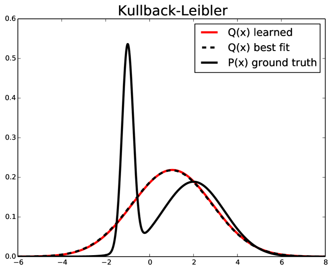
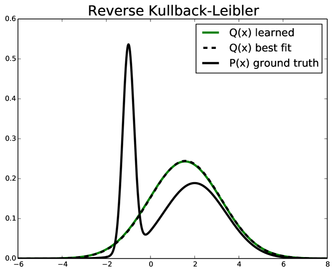
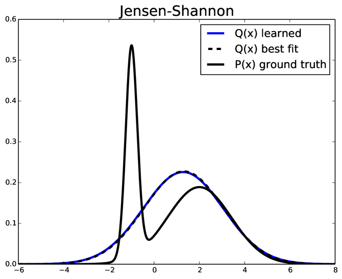
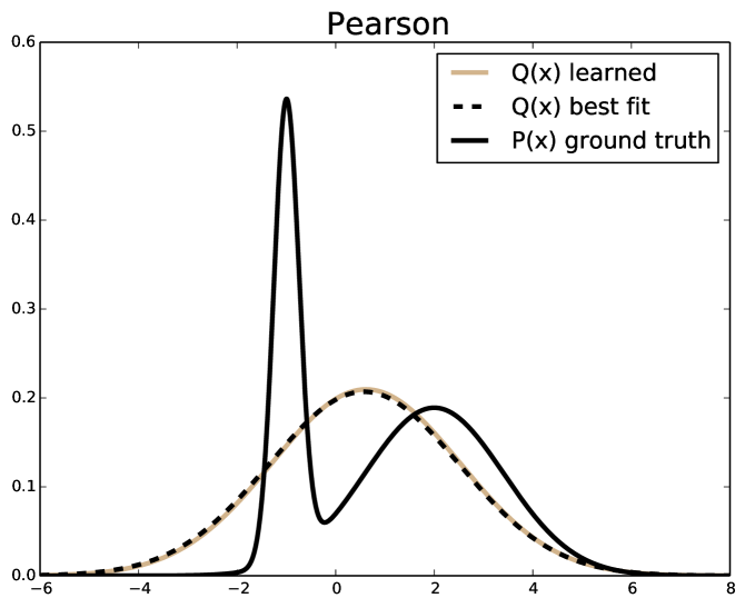
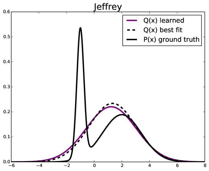
Setup. We approximate a mixture of Gaussian by learning a Gaussian distribution. The model $Q_{\theta}$ is represented by a linear function which receives a random $z\sim\mathcal{N}(0,1)$ and outputs

$$G_{\theta}(z)=\mu+\sigma z,$$ (19)

where $\theta=(\mu,\sigma)$ are the parameters to be learned. For the variational function $T_{\omega}$ we use the neural network

$$x \to\textrm{Linear(1,64)}\to\textrm{Tanh}\to\textrm{Linear(64,64)}\to\textrm{Tanh}\to\textrm{Linear(64,1)}.$$ (20)

We optimise the objective $F(\omega,\theta)$ by using the single-step gradient method presented in Section 3.1 of the main text . In each step we sample batches of size $1024$ each for both $p(x)$ and $p(z)$ and we use a step-size of $0.01$ for updating both $\omega$ and $\theta$. We compare the results to the best fit provided by the exact optimisation of $D_{f}(P\|Q_{\theta})$ w.r.t. $\theta$, which is feasible in this case by solving the required integrals numerically. We use $(\hat{\omega},\hat{\theta})$ (learned) and $\theta^{\ast}$ (best fit) to distinguish the parameters sets used in these two approaches.

Results. The panels in Figure 5 shows the density function of the data distribution as well as the Gaussian approximations corresponding to a few $f$-divergences form Table 5. As expected, the KL approximation covers the data distribution by fitting its mean and variance while KL-rev has more of a mode-seeking behavior [24]. The fit corresponding to the Jensen-Shannon divergence is somewhere between KL and KL-rev. All Gaussian approximations resulting from neural network training are close to the ones obtained by direct optimisation of the divergence (learned vs. best fit).

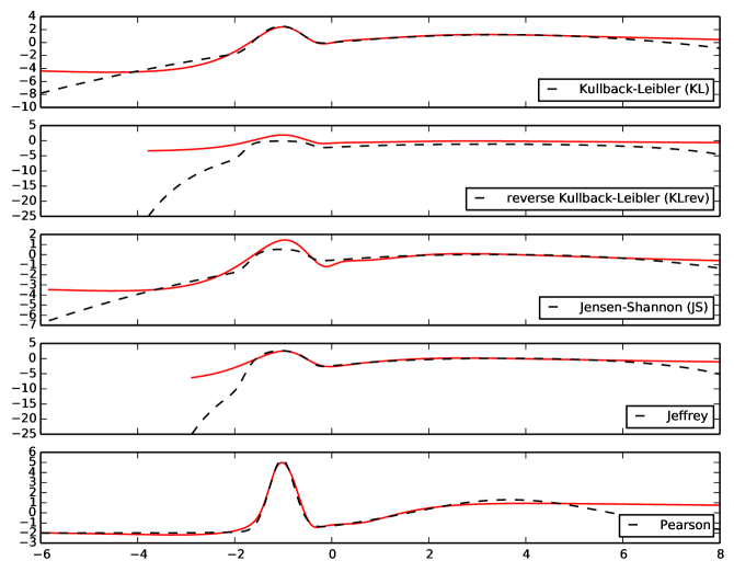
In the right–bottom panel of Figure 5 we compare the variational functions $T_{\hat{\omega}}$ and $T^{\ast}$. The latter is defined as $T^{\ast}(x)=f^{\prime}(p(x)/q_{{\theta}^{\ast}}(x))$, see main text. The objective value corresponding to $T^{\ast}$ is the true divergence $D_{f}(P\rvert\lvert Q_{{\theta}^{\ast}})$. In the majority of the cases our $T_{\hat{\omega}}$ is close to $T^{\ast}$ in the area of interest. The discrepancies around the tails are due to the fact that (1) the class of functions resulting from the $\rm tanh$ activation function has limited capability representing the tails, and (2) in the Gaussian case there is a lack of data in the tails. These limitations, however, do not have a significant effect on the learned parameters.

Appendix F Details of the Experiments

In this section we present the technical setup as well as the architectures we used in the experiments described in Section 4.

F.1 Deep Learning Environment

We use the deep learning framework Chainer [32], version 1.8.1, running on CUDA 7.5 with CuDNN v5 on NVIDIA GTX TITAN X.

F.2 MNIST Setup

MNIST Generator

$$z \to\textrm{Linear(100, 1200)}\to\textrm{BN}\to\textrm{ReLU}\to\textrm{Linear(1200, 1200)}\to\textrm{BN}\to\textrm{ReLU}$$ (21)

$$\to\textrm{Linear(1200, 784)}\to\textrm{Sigmoid}$$

All weights are initialized at a weight scale of $0.05$, as in [10].

MNIST Variational Function

$$x \to\textrm{Linear(784,240)}\to\textrm{ELU}\to\textrm{Linear(240,240)}\to\textrm{ELU}\to\textrm{Linear(240,1)},$$ (22)

where ELU is the exponential linear unit [4]. All weights are initialized at a weight scale of $0.005$, one order of magnitude smaller than in [10].

Variational Autoencoders

For the variational autoencoders [18], we used the example implementation included with Chainer [32]. We trained for 100 epochs with 20 latent dimensions.

F.3 LSUN Natural Images

$$z \to\textrm{Linear(100, $6\cdot 6\cdot 512$)}\to\textrm{BN}\to\textrm{ReLU}\to\textrm{Reshape(512,6,6)}$$ (23)

$$\to\textrm{Deconv(512,256)}\to\textrm{BN}\to\textrm{ReLU}\to\textrm{Deconv(256,128)}\to\textrm{BN}\to\textrm{ReLU}$$

$$\to\textrm{Deconv(128,64)}\to\textrm{BN}\to\textrm{ReLU}\to\textrm{Deconv(64,3)},$$

where all Deconv operations use a kernel size of four and a stride of two.

References

- Ali and Silvey [1966] S. M. Ali and S. D. Silvey. A general class of coefficients of divergence of one distribution from another. JRSS (B), pages 131–142, 1966.
- Bishop [1994] C. M. Bishop. Mixture density networks. Technical report, Aston University, 1994.
- Bishop et al. [1998] C. M. Bishop, M. Svensén, and C. K. I. Williams. GTM: The generative topographic mapping. Neural Computation, 10(1):215–234, 1998.
- Clevert et al. [2015] D. A. Clevert, T. Unterthiner, and S. Hochreiter. Fast and accurate deep network learning by exponential linear units (ELUs). arXiv:1511.07289, 2015.
- Csiszár and Shields [2004] I. Csiszár and P. C. Shields. Information theory and statistics: A tutorial. Foundations and Trends in Communications and Information Theory, 1:417–528, 2004.
- Dauphin et al. [2014] Y. N. Dauphin, R. Pascanu, C. Gulcehre, K. Cho, S. Ganguli, and Y. Bengio. Identifying and attacking the saddle point problem in high-dimensional non-convex optimization. In NIPS, pages 2933–2941, 2014.
- Dziugaite et al. [2015] G. K. Dziugaite, D. M. Roy, and Z. Ghahramani. Training generative neural networks via maximum mean discrepancy optimization. In UAI, pages 258–267, 2015.
- Gauthier [2014] J. Gauthier. Conditional generative adversarial nets for convolutional face generation. Class Project for Stanford CS231N: Convolutional Neural Networks for Visual Recognition, Winter semester 2014, 2014.
- Gneiting and Raftery [2007] T. Gneiting and A. E. Raftery. Strictly proper scoring rules, prediction, and estimation. JASA, 102(477):359–378, 2007.
- Goodfellow et al. [2014] I. Goodfellow, J. Pouget-Abadie, M. Mirza, B. Xu, D. Warde-Farley, S. Ozair, A. Courville, and Y. Bengio. Generative adversarial nets. In NIPS, pages 2672–2680, 2014.
- Graves [2013] A. Graves. Generating sequences with recurrent neural networks. arXiv:1308.0850, 2013.
- Gretton et al. [2007] A. Gretton, K. Fukumizu, C. H. Teo, L. Song, B. Schölkopf, and A. J. Smola. A kernel statistical test of independence. In NIPS, pages 585–592, 2007.
- Gutmann and Hyvärinen [2010] M. Gutmann and A. Hyvärinen. Noise-contrastive estimation: A new estimation principle for unnormalized statistical models. In AISTATS, pages 297–304, 2010.
- Hiriart-Urruty and Lemaréchal [2012] J. B. Hiriart-Urruty and C. Lemaréchal. Fundamentals of convex analysis. Springer, 2012.
- [15] F. Huszár. An alternative update rule for generative adversarial networks. http://www.inference.vc/an-alternative-update-rule-for-generative-adversarial-networks/.
- Huszár [2015] F. Huszár. How (not) to train your generative model: scheduled sampling, likelihood, adversary? arXiv:1511.05101, 2015.
- Kingma and Ba [2014] D. Kingma and J. Ba. Adam: A method for stochastic optimization. arXiv:1412.6980, 2014.
- Kingma and Welling [2013] D. P. Kingma and M. Welling. Auto-encoding variational Bayes. arXiv:1402.0030, 2013.
- Larochelle and Murray [2011] H. Larochelle and I. Murray. The neural autoregressive distribution estimator. In AISTATS, 2011.
- Li et al. [2015] Y. Li, K. Swersky, and R. Zemel. Generative moment matching networks. In ICML, 2015.
- Liese and Vajda [2006] F. Liese and I. Vajda. On divergences and informations in statistics and information theory. Information Theory, IEEE, 52(10):4394–4412, 2006.
- MacKay [1995] D. J. C. MacKay. Bayesian neural networks and density networks. Nucl. Instrum. Meth. A, 354(1):73–80, 1995.
- Makhzani et al. [2015] A. Makhzani, J. Shlens, N. Jaitly, and I. Goodfellow. Adversarial autoencoders. arXiv:1511.05644, 2015.
- Minka [2005] T. Minka. Divergence measures and message passing. Technical report, Microsoft Research, 2005.
- Nguyen et al. [2010] X. Nguyen, M. J. Wainwright, and M. I. Jordan. Estimating divergence functionals and the likelihood ratio by convex risk minimization. Information Theory, IEEE, 56(11):5847–5861, 2010.
- Nielsen and Nock [2014] F. Nielsen and R. Nock. On the chi-square and higher-order chi distances for approximating f-divergences. Signal Processing Letters, IEEE, 21(1):10–13, 2014.
- Radford et al. [2015] A. Radford, L. Metz, and S. Chintala. Unsupervised representation learning with deep convolutional generative adversarial networks. arXiv:1511.06434, 2015.
- Rezende et al. [2014] D. J. Rezende, S. Mohamed, and D. Wierstra. Stochastic backpropagation and approximate inference in deep generative models. In ICML, pages 1278–1286, 2014.
- Sohl-Dickstein et al. [2015] J. Sohl-Dickstein, E. A. Weiss, N. Maheswaranathan, and S. Ganguli. Deep unsupervised learning using non-equilibrium thermodynamics. ICML, pages 2256––2265, 2015.
- Sriperumbudur et al. [2010] B. K. Sriperumbudur, A. Gretton, K. Fukumizu, B. Schölkopf, and G. Lanckriet. Hilbert space embeddings and metrics on probability measures. JMLR, 11:1517–1561, 2010.
- Theis et al. [2015] L. Theis, A. v.d. Oord, and M. Bethge. A note on the evaluation of generative models. arXiv:1511.01844, 2015.
- Tokui et al. [2015] S. Tokui, K. Oono, S. Hido, and J. Clayton. Chainer: a next-generation open source framework for deep learning. In NIPS, 2015.
- Uria et al. [2013] B. Uria, I. Murray, and H. Larochelle. RNADE: The real-valued neural autoregressive density-estimator. In NIPS, pages 2175–2183, 2013.
- Yu et al. [2015] F. Yu, Y. Zhang, S. Song, A. Seff, and J. Xiao. LSUN: Construction of a large-scale image dataset using deep learning with humans in the loop. arXiv:1506.03365, 2015.