Adversarially Learned Inference

Abstract

We introduce the adversarially learned inference (ALI) model, which jointly learns a generation network and an inference network using an adversarial process. The generation network maps samples from stochastic latent variables to the data space while the inference network maps training examples in data space to the space of latent variables. An adversarial game is cast between these two networks and a discriminative network is trained to distinguish between joint latent/data-space samples from the generative network and joint samples from the inference network. We illustrate the ability of the model to learn mutually coherent inference and generation networks through the inspections of model samples and reconstructions and confirm the usefulness of the learned representations by obtaining a performance competitive with state-of-the-art on the semi-supervised SVHN and CIFAR10 tasks.

1 Introduction

Deep directed generative model has emerged as a powerful framework for modeling complex high-dimensional datasets. These models permit fast ancestral sampling, but are often challenging to learn due to the complexities of inference. Recently, three classes of algorithms have emerged as effective for learning deep directed generative models: 1) techniques based on the Variational Autoencoder (VAE) that aim to improve the quality and efficiency of inference by learning an inference machine (Kingma & Welling, 2013; Rezende et al., 2014), 2) techniques based on Generative Adversarial Networks (GANs) that bypass inference altogether (Goodfellow et al., 2014) and 3) autoregressive approaches (van den Oord et al., 2016b; c; a) that forego latent representations and instead model the relationship between input variables directly. While all techniques are provably consistent given infinite capacity and data, in practice they learn very different kinds of generative models on typical datasets.

VAE-based techniques learn an approximate inference mechanism that allows reuse for various auxiliary tasks, such as semi-supervised learning or inpainting. They do however suffer from a well-recognized issue of the maximum likelihood training paradigm when combined with a conditional independence assumption on the output given the latent variables: they tend to distribute probability mass diffusely over the data space (Theis et al., 2015). The direct consequence of this is that image samples from VAE-trained models tend to be blurry (Goodfellow et al., 2014; Larsen et al., 2015). Autoregressive models produce outstanding samples but do so at the cost of slow sampling speed and foregoing the learning of an abstract representation of the data. GAN-based approaches represent a good compromise: they learn a generative model that produces higher-quality samples than the best VAE techniques (Radford et al., 2015; Larsen et al., 2015) without sacrificing sampling speed and also make use of a latent representation in the generation process. However, GANs lack an efficient inference mechanism, which prevents them from reasoning about data at an abstract level. For instance, GANs don’t allow the sort of neural photo manipulations showcased in (Brock et al., 2016). Recently, efforts have aimed to bridge the gap between VAEs and GANs, to learn generative models with higher-quality samples while learning an efficient inference network (Larsen et al., 2015; Lamb et al., 2016; Dosovitskiy & Brox, 2016). While this is certainly a promising research direction, VAE-GAN hybrids tend to manifest a compromise of the strengths and weaknesses of both approaches.

In this paper, we propose a novel approach to integrate efficient inference within the GAN framework. Our approach, called Adversarially Learned Inference (ALI), casts the learning of both an inference machine (or encoder) and a deep directed generative model (or decoder) in an GAN-like adversarial framework. A discriminator is trained to discriminate joint samples of the data and the corresponding latent variable from the encoder (or approximate posterior) from joint samples from the decoder while in opposition, the encoder and the decoder are trained together to fool the discriminator. Not only are we asking the discriminator to distinguish synthetic samples from real data, but we are requiring it to distinguish between two joint distributions over the data space and the latent variables.

With experiments on the Street View House Numbers (SVHN) dataset (Netzer et al., 2011), the CIFAR-10 object recognition dataset (Krizhevsky & Hinton, 2009), the CelebA face dataset (Liu et al., 2015) and a downsampled version of the ImageNet dataset (Russakovsky et al., 2015), we show qualitatively that we maintain the high sample fidelity associated with the GAN framework, while gaining the ability to perform efficient inference. We show that the learned representation is useful for auxiliary tasks by achieving results competitive with the state-of-the-art on the semi-supervised SVHN and CIFAR10 tasks.

2 Adversarially learned inference

Figure 1: The adversarially learned inference (ALI) game.

Consider the two following probability distributions over $\bm{x}$ and $\bm{z}$:

• the encoder joint distribution $q(\bm{x},\bm{z})=q(\bm{x})q(\bm{z}\mid\bm{x})$,

• the decoder joint distribution $p(\bm{x},\bm{z})=p(\bm{z})p(\bm{x}\mid\bm{z})$.

These two distributions have marginals that are known to us: the encoder marginal $q(\bm{x})$ is the empirical data distribution and the decoder marginal $p(\bm{z})$ is usually defined to be a simple, factorized distribution, such as the standard Normal distribution $p(\bm{z})=\mathcal{N}(\bm{0},\bm{I})$. As such, the generative process between $q(\bm{x},\bm{z})$ and $p(\bm{x},\bm{z})$ is reversed.

ALI’s objective is to match the two joint distributions. If this is achieved, then we are ensured that all marginals match and all conditional distributions also match. In particular, we are assured that the conditional $q(\bm{z}\mid\bm{x})$ matches the posterior $p(\bm{z}\mid\bm{x})$.

In order to match the joint distributions, an adversarial game is played. Joint pairs $(\bm{x},\bm{z})$ are drawn either from $q(\bm{x},\bm{z})$ or $p(\bm{x},\bm{z})$, and a discriminator network learns to discriminate between the two, while the encoder and decoder networks are trained to fool the discriminator.

The value function describing the game is given by:

$$\begin{split}\min_{G}\max_{D}V(D,G)&=\mathbb{E}_{q(\bm{x})}[\log(D(\bm{x},G_{z}(\bm{x})))]+\mathbb{E}_{p(\bm{z})}[\log(1-D(G_{x}(\bm{z}),\bm{z}))]\\ &=\iint q(\bm{x})q(\bm{z}\mid\bm{x})\log(D(\bm{x},\bm{z}))d\bm{x}d\bm{z}\\ &+\iint p(\bm{z})p(\bm{x}\mid\bm{z})\log(1-D(\bm{x},\bm{z}))d\bm{x}d\bm{z}.\end{split}$$ (1)

An attractive property of adversarial approaches is that they do not require that the conditional densities can be computed; they only require that they can be sampled from in a way that allows gradient backpropagation. In the case of ALI, this means that gradients should propagate from the discriminator network to the encoder and decoder networks.

This can be done using the the reparametrization trick (Kingma, 2013; Bengio et al., 2013b; a). Instead of sampling directly from the desired distribution, the random variable is computed as a deterministic transformation of some noise such that its distribution is the desired distribution. For instance, if $q(z\mid x)=\mathcal{N}(\mu(x),\sigma^{2}(x)I)$, one can draw samples by computing

$$z=\mu(x)+\sigma(x)\odot\epsilon,\quad\epsilon\sim\mathcal{N}(0,I).$$ (2)

More generally, one can employ a change of variable of the form

$$v=f(u,\epsilon)$$ (3)

where $\epsilon$ is some random source of noise.

The discriminator is trained to distinguish between samples from the encoder $(\bm{x},\hat{\bm{z}})\sim q(\bm{x},\bm{z})$ and samples from the decoder $(\tilde{\bm{x}},\bm{z})\sim p(\bm{x},\bm{z})$. The generator is trained to fool the discriminator, i.e., to generate $\bm{x},\bm{z}$ pairs from $q(\bm{x},\bm{z})$ or $p(\bm{x},\bm{z})$ that are indistinguishable one from another. See Figure 1 for a diagram of the adversarial game and Algorithm 1 for an algorithmic description of the procedure.

In such a setting, and under the assumption of an optimal discriminator, the generator minimizes the Jensen-Shannon divergence (Lin, 1991) between $q(\bm{x},\bm{z})$ and $p(\bm{x},\bm{z})$. This can be shown using the same proof sketch as in the original GAN paper (Goodfellow et al., 2014).

$\theta_{g},\theta_{d}\leftarrow\text{initialize network parameters}$

repeat

     $\bm{x}^{(1)},\ldots,\bm{x}^{(M)}\sim q(\bm{x})$ $\triangleright$ Draw $M$ samples from the dataset and the prior

     $\bm{z}^{(1)},\ldots,\bm{z}^{(M)}\sim p(\bm{z})$

     $\hat{\bm{z}}^{(i)}\sim q(\bm{z}\mid\bm{x}=\bm{x}^{(i)}),\quad i=1,\ldots,M$ $\triangleright$ Sample from the conditionals

     $\tilde{\bm{x}}^{(j)}\sim p(\bm{x}\mid\bm{z}=\bm{z}^{(j)}),\quad j=1,\ldots,M$

     $\rho_{q}^{(i)}\leftarrow D(\bm{x}^{(i)},\hat{\bm{z}}^{(i)}),\quad i=1,\ldots,M$ $\triangleright$ Compute discriminator predictions

     $\rho_{p}^{(j)}\leftarrow D(\tilde{\bm{x}}^{(j)},\bm{z}^{(j)}),\quad j=1,\ldots,M$

     $\mathcal{L}_{d}\leftarrow-\frac{1}{M}\sum_{i=1}^{M}\log(\rho_{q}^{(i)})-\frac{1}{M}\sum_{j=1}^{M}\ log(1-\rho_{p}^{(j)})$ $\triangleright$ Compute discriminator loss

     $\mathcal{L}_{g}\leftarrow-\frac{1}{M}\sum_{i=1}^{M}\log(1-\rho_{q}^{(i)})-\frac{1}{M}\sum_{j=1}^{M}\log(\rho_{p}^{(j)})$ $\triangleright$ Compute generator loss

     $\theta_{d}\leftarrow\theta_{d}-\nabla_{\theta_{d}}\mathcal{L}_{d}$ $\triangleright$ Gradient update on discriminator network

     $\theta_{g}\leftarrow\theta_{g}-\nabla_{\theta_{g}}\mathcal{L}_{g}$ $\triangleright$ Gradient update on generator networks

until convergence

Algorithm 1 The ALI training procedure.

2.1 Relation to GAN

ALI bears close resemblance to GAN, but it differs from it in the two following ways:

• The generator has two components: the encoder, $G_{z}(\bm{x})$, which maps data samples $\bm{x}$ to $\bm{z}$-space, and the decoder $G_{x}(\bm{z})$, which maps samples from the prior $p(\bm{z})$ (a source of noise) to the input space.

• The discriminator is trained to distinguish between joint pairs $(\bm{x},\hat{\bm{z}}=G_{x}(\bm{x}))$ and $(\tilde{\bm{x}}=G_{x}(\bm{z}),\bm{z})$, as opposed to marginal samples $\bm{x}\sim q(\bm{x})$ and $\tilde{\bm{x}}\sim p(\bm{x})$.

2.2 Alternative approaches to feedforward inference in GANs

The ALI training procedure is not the only way one could learn a feedforward inference network in a GAN setting.

In recent work, Chen et al. (2016) introduce a model called InfoGAN which minimizes the mutual information between a subset $\bm{c}$ of the latent code and $\bm{x}$ through the use of an auxiliary distribution $Q(\bm{c}\mid\bm{x})$. However, this does not correspond to full inference on $\bm{z}$, as only the value for $\bm{c}$ is inferred. Additionally, InfoGAN requires that $Q(\bf{c}\mid\bf{x})$ is a tractable approximate posterior that can be sampled from and evaluated. ALI only requires that inference networks can be sampled from, allowing it to represent arbitrarily complex posterior distributions.

One could learn the inverse mapping from GAN samples: this corresponds to learning an encoder to reconstruct $\bm{z}$, i.e. finding an encoder such that $\mathbb{E}_{z\sim p(z)}[\|z-G_{z}(G_{x}(z))\|_{2}^{2}]\approx 0$. We are not aware of any work that reports results for this approach. This resembles the InfoGAN learning procedure but with a fixed generative model and a factorial Gaussian posterior with a fixed diagonal variance.

Alternatively, one could decompose training into two phases. In the first phase, a GAN is trained normally. In the second phase, the GAN’s decoder is frozen and an encoder is trained following the ALI procedure (i.e., a discriminator taking both $\bm{x}$ and $\bm{z}$ as input is introduced). We call this post-hoc learned inference. In this setting, the encoder and the decoder cannot interact together during training and the encoder must work with whatever the decoder has learned during GAN training. Post-hoc learned inference may be suboptimal if this interaction is beneficial to modeling the data distribution.

2.3 Generator value function

As with GANs, when ALI’s discriminator gets too far ahead, its generator may have a hard time minimizing the value function in Equation 1. If the discriminator’s output is sigmoidal, then the gradient of the value function with respect to the discriminator’s output vanishes to zero as the output saturates.

As a workaround, the generator is trained to maximize

$$V^{\prime}(D,G)=\mathbb{E}_{q(\bm{x})}[\log(1-D(\bm{x},G_{\bm{z}}(\bm{x})))]+\mathbb{E}_{p(\bm{z})}[\log(D(G_{\bm{x}}(\bm{z}),\bm{z}))]\\$$ (4)

which has the same fixed points but whose gradient is stronger when the discriminator’s output saturates.

The adversarial game does not require an analytical expression for the joint distributions. This means we can introduce variable changes without having to know the explicit distribution over the new variable. For instance, sampling from $p(z)$ could be done by sampling $\epsilon\sim\mathcal{N}(0,I)$ and passing it through an arbitrary differentiable function $z=f(\epsilon)$.

However, gradient propagation into the encoder and decoder networks relies on the reparametrization trick, which means that ALI is not directly applicable to either applications with discrete data or to models with discrete latent variables.

(a) SVHN samples.

(b) SVHN reconstructions.

Figure 2: Samples and reconstructions on the SVHN dataset. For the reconstructions, odd columns are original samples from the validation set and even columns are corresponding reconstructions (e.g., second column contains reconstructions of the first column’s validation set samples).

(a) CelebA samples.

(b) CelebA reconstructions.

Figure 3: Samples and reconstructions on the CelebA dataset. For the reconstructions, odd columns are original samples from the validation set and even columns are corresponding reconstructions.

(a) CIFAR10 samples.

(b) CIFAR10 reconstructions.

Figure 4: Samples and reconstructions on the CIFAR10 dataset. For the reconstructions, odd columns are original samples from the validation set and even columns are corresponding reconstructions.

2.4 Discriminator optimality

Proposition 1.

Given a fixed generator $G$, the optimal discriminator is given by

$$D^{*}(x,z)=\frac{q(x,z)}{q(x,z)+p(x,z)}.$$ (5)

Proof.

For a fixed generator $G$, the complete data value function is

$$V(D,G)=\mathbb{E}_{x,z\sim q(x,z)}[\log(D(x,z))]+\mathbb{E}_{x,z\sim p(x,z)}[\log(1-D(x,z))].$$ (6)

The result follows by the concavity of the log and the simplified Euler-Lagrange equation first order conditions on $(x,z)\rightarrow D(x,z)$. ∎

2.5 Relationship with the Jensen-Shannon divergence

Proposition 2.

Under an optimal discriminator $D^{*}$, the generator minimizes the Jensen-Shanon divergence which attains its minimum if and only if $q(\bm{x},\bm{z})=p(\bm{x},\bm{z})$.

Proof.

The proof is a straightforward extension of the proof in Goodfellow et al. (2014). ∎

2.6 Invertibility

Proposition 3.

Assuming optimal discriminator $D$ and generator $G$. If the encoder $G_{\bm{x}}$ is deterministic, then $G_{\bm{x}}=G^{-1}_{\bm{z}}$ and $G_{\bm{z}}=G^{-1}_{\bm{x}}$ almost everywhere.

Sketch of proof.

Consider the event $R_{\epsilon}=\{\bm{x}:\|x-(G_{\bm{x}}\circ G_{\bm{z}})(\bm{x}))\|>\epsilon\}$ for some positive $\epsilon$. This set can be seen as a section of the $(\bm{x},\bm{z})$ space over the elements $\bm{z}$ such that $\bm{z}=G_{\bm{z}}(x)$. The generator being optimal, the probabilities of $R_{\epsilon}$ under $p(\bm{x},\bm{z})$ and $q(\bm{x},\bm{z})$ are equal. Now $p(\bm{x}\mid\bm{z})=\delta_{x-G_{x}(z)}$, where $\delta$ is the Dirac delta distribution. This is enough to show that there are no $x$ satisfying the event $R_{\epsilon}$ and thus $G_{\bm{x}}=G^{-1}_{z}$ almost everywhere. By symmetry, the same argument can be applied to show that $G_{\bm{z}}=G^{-1}_{\bm{x}}$.
The complete proof is given in (Donahue et al., 2016), in which the authors independently examine the same model structure under the name Bidirectional GAN (BiGAN). ∎

3 Related Work

Other recent papers explore hybrid approaches to generative modeling. One such approach is to relax the probabilistic interpretation of the VAE model by replacing either the KL-divergence term or the reconstruction term with variants that have better properties. The adversarial autoencoder model (Makhzani et al., 2015) replaces the KL-divergence term with a discriminator that is trained to distinguish between approximate posterior and prior samples, which provides a more flexible approach to matching the marginal $q(\bm{z})$ and the prior. Other papers explore replacing the reconstruction term with either GANs or auxiliary networks. Larsen et al. (2015) collapse the decoder of a VAE and the generator of a GAN into one network in order to supplement the reconstruction loss with a learned similarity metric. Lamb et al. (2016) use the hidden layers of a pre-trained classifier as auxiliary reconstruction losses to help the VAE focus on higher-level details when reconstructing. Dosovitskiy & Brox (2016) combine both ideas into a unified loss function.

ALI’s approach is also reminiscent of the adversarial autoencoder model, which employs a GAN to distinguish between samples from the approximate posterior distribution $q(\bm{z}\mid\bm{x})$ and prior samples. However, unlike adversarial autoencoders, no explicit reconstruction loss is being optimized in ALI, and the discriminator receives joint pairs of samples $(\bm{x},\bm{z})$ rather than marginal $\bm{z}$ samples.

Independent work by Donahue et al. (2016) proposes the same model under the name Bidirectional GAN (BiGAN), in which the authors emphasize the learned features’ usefulness for auxiliary supervised and semi-supervised tasks. The main difference in terms of experimental setting is that they use a deterministic $q(\bm{z}\mid\bm{x})$ network, whereas we use a stochastic network. In our experience, this does not make a big difference when $\bm{x}$ is a deterministic function of $\bm{z}$ as the stochastic inference networks tend to become determinstic as training progresses. When using stochastic mappings from $\bm{z}$ to $\bm{x}$, the additional flexiblity of stochastic posteriors is critical.

4 Experimental results

(a) Tiny ImageNet samples.

(b) Tiny ImageNet reconstructions.

Figure 5: Samples and reconstructions on the Tiny ImageNet dataset. For the reconstructions, odd columns are original samples from the validation set and even columns are corresponding reconstructions.

We applied ALI to four different datasets, namely CIFAR10 (Krizhevsky & Hinton, 2009), SVHN (Netzer et al., 2011), CelebA (Liu et al., 2015) and a center-cropped, $64\times 64$ version of the ImageNet dataset (Russakovsky et al., 2015).

Transposed convolutions are used in $G_{x}(\bm{z})$. This operation corresponds to the transpose of the matrix representation of a convolution, i.e., the gradient of the convolution with respect to its inputs. For more details about transposed convolutions and related operations, see Dumoulin & Visin (2016); Shi et al. (2016); Odena et al. (2016).

4.1 Samples and Reconstructions

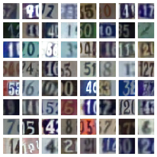
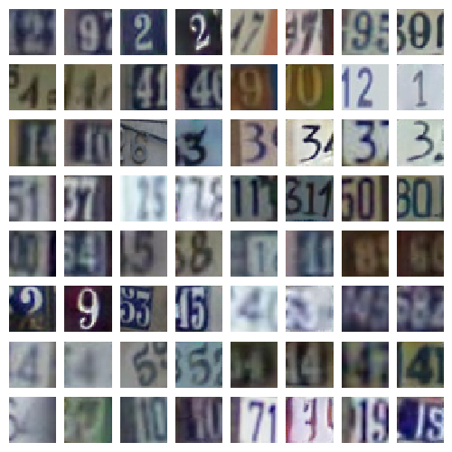
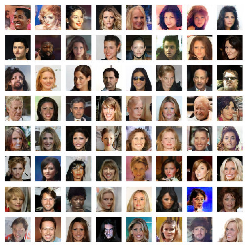
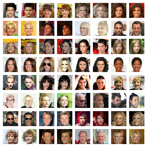
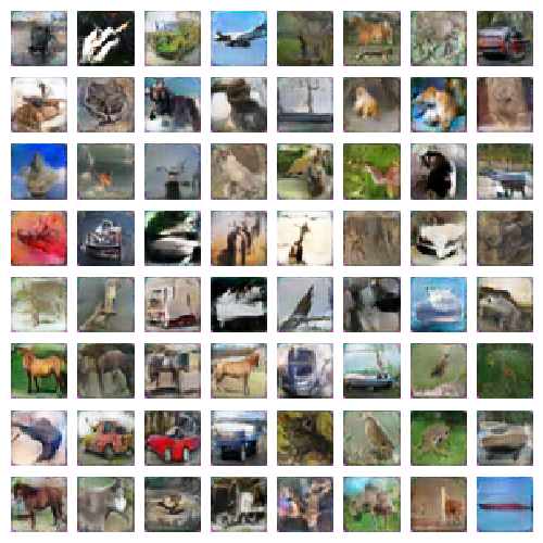
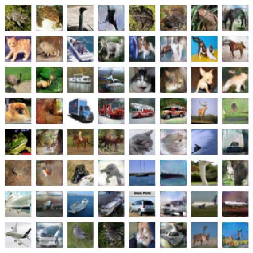
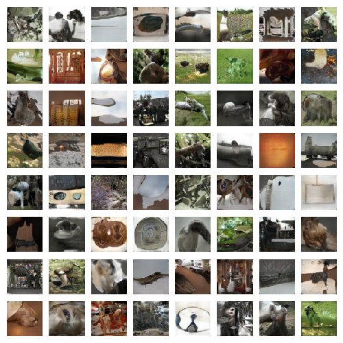
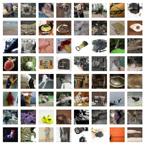
For each dataset, samples are presented (Figures 2(a), 3(a) 4(a) and 5(a)). They exhibit the same image fidelity as samples from other adversarially-trained models.

We also qualitatively evaluate the fit between the conditional distribution $q(\bm{z}\mid\bm{x})$ and the posterior distribution $p(\bm{z}\mid\bm{x})$ by sampling $\hat{\bm{z}}\sim q(\bm{z}\mid\bm{x})$ and $\hat{\bm{x}}\sim p(\bm{x}\mid\bm{z}=\hat{\bm{z}})$ (Figures 2(b), 3(b), 4(b) and 5(b)). This corresponds to reconstructing the input in a VAE setting. Note that the ALI training objective does not involve an explicit reconstruction loss.

We observe that reconstructions are not always faithful reproductions of the inputs. They retain the same crispness and quality characteristic to adversarially-trained models, but oftentimes make mistakes in capturing exact object placement, color, style and (in extreme cases) object identity. The extent to which reconstructions deviate from the inputs varies between datasets: on CIFAR10, which arguably constitutes a more complex input distribution, the model exhibits less faithful reconstructions. This leads us to believe that poor reconstructions are a sign of underfitting.

This failure mode represents an interesting departure from the bluriness characteristic to the typical VAE setup. We conjecture that in the underfitting regime, the latent variable representation learned by ALI is potentially more invariant to less interesting factors of variation in the input and do not devote model capacity to capturing these factors.

4.2 Latent space interpolations

As a sanity check for overfitting, we look at latent space interpolations between validation set examples (Figure 6). We sample pairs of validation set examples $\mathbf{x}_{1}$ and $\mathbf{x}_{2}$ and project them into $\mathbf{z}_{1}$ and $\mathbf{z}_{2}$ by sampling from the encoder. We then linearly interpolate between $\mathbf{z}_{1}$ and $\mathbf{z}_{2}$ and pass the intermediary points through the decoder to plot the input-space interpolations.

We observe smooth transitions between pairs of examples, and intermediary images remain believable. This is an indicator that ALI is not concentrating its probability mass exclusively around training examples, but rather has learned latent features that generalize well.

Figure 6: Latent space interpolations on the CelebA validation set. Left and right columns correspond to the original pairs $\mathbf{x}_{1}$ and $\mathbf{x}_{2}$, and the columns in between correspond to the decoding of latent representations interpolated linearly from $\mathbf{z}_{1}$ to $\mathbf{z}_{2}$. Unlike other adversarial approaches like DCGAN (Radford et al., 2015), ALI allows one to interpolate between actual data points.

4.3 Semi-supervised learning

We investigate the usefulness of the latent representation learned by ALI through semi-supervised benchmarks on SVHN and CIFAR10.

We first compare with GAN on SVHN by following the procedure outlined in Radford et al. (2015). We train an L2-SVM on the learned representations of a model trained on SVHN. The last three hidden layers of the encoder as well as its output are concatenated to form a 8960-dimensional feature vector. A 10,000 example held-out validation set is taken from the training set and is used for model selection. The SVM is trained on 1000 examples taken at random from the remainder of the training set. The test error rate is measured for 100 different SVMs trained on different random 1000-example training sets, and the average error rate is measured along with its standard deviation.

Using ALI’s inference network as opposed to the discriminator to extract features, we achieve a misclassification rate that is roughly $3.00\pm 0.50\%$ lower than reported in Radford et al. (2015) (Table 1), which suggests that ALI’s inference mechanism is beneficial to the semi-supervised learning task.

We then investigate ALI’s performance when label information is taken into account during training. We adapt the discriminative model proposed in Salimans et al. (2016). The discriminator takes $x$ and $z$ as input and outputs a distribution over $K+1$ classes, where $K$ is the number of categories. When label information is available for $q(x,z)$ samples, the discriminator is expected to predict the label. When no label information is available, the discriminator is expected to predict $K+1$ for $p(x,z)$ samples and $k\in\{1,\ldots,K\}$ for $q(x,z)$ samples.

Interestingly, Salimans et al. (2016) found that they required an alternative training strategy for the generator where it tries to match first-order statistics in the discriminator’s intermediate activations with respect to the data distribution (they refer to this as feature matching). We found that ALI did not require feature matching to obtain comparable results. We achieve results competitive with the state-of-the-art, as shown in Tables 1 and 2. Table 2 shows that ALI offers a modest improvement over Salimans et al. (2016), more specifically for 1000 and 2000 labeled examples.

Table 1: SVHN test set missclassification rate

. Model Misclassification rate VAE (M1 + M2) (Kingma et al., 2014) $36.02$ SWWAE with dropout (Zhao et al., 2015) $23.56$ DCGAN + L2-SVM (Radford et al., 2015) $22.18$ SDGM (Maaløe et al., 2016) $16.61$ GAN (feature matching) (Salimans et al., 2016) $\mathbf{8.11\pm 1.3}$ ALI (ours, L2-SVM) $19.14\pm 0.50$ ALI (ours, no feature matching) $\mathbf{7.42\pm 0.65}$

Table 2: CIFAR10 test set missclassification rate for semi-supervised learning using different numbers of trained labeled examples. For ALI, error bars correspond to 3 times the standard deviation.

Number of labeled examples	1000	2000	4000	8000
Model	Misclassification rate
Ladder network (Rasmus et al., 2015)			$20.40$
CatGAN (Springenberg, 2015)			$19.58$
GAN (feature matching) (Salimans et al., 2016)	$\mathbf{21.83\pm 2.01}$	$\mathbf{19.61\pm 2.09}$	$\mathbf{18.63\pm 2.32}$	$\mathbf{17.72\pm 1.82}$
ALI (ours, no feature matching)	$\mathbf{19.98\pm 0.89}$	$\mathbf{19.09\pm 0.44}$	$\mathbf{17.99\pm 1.62}$	$\mathbf{17.05\pm 1.49}$

We are still investigating the differences between ALI and GAN with respect to feature matching, but we conjecture that the latent representation learned by ALI is better untangled with respect to the classification task and that it generalizes better.

4.4 Conditional Generation

We extend ALI to match a conditional distribution. Let $\bm{y}$ represent a fully observed conditioning variable. In this setting, the value function reads

$$\min_{G}\max_{D}V(D,G)=\mathbb{E}_{q(\bm{x})\,p(\bm{y})}[\log(D(\bm{x},G_{z}(\bm{x},\bm{y}),\bm{y}))]+\mathbb{E}_{p(\bm{z})\,p(\bm{y})}[\log(1-D(G_{x}(\bm{z},\bm{y}),\bm{z},\bm{y}))]$$ (7)

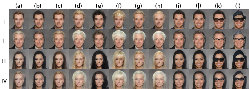
We apply the conditional version of ALI to CelebA using the dataset’s 40 binary attributes. The attributes are linearly embedded in the encoder, decoder and discriminator. We observe how a single element of the latent space $z$ changes with respect to variations in the attributes vector $y$. Conditional samples are shown in Figure 7.

Figure 7: Conditional generation sequence. We sample a single fixed latent code $z$. Each row has a subset of attributes that are held constant across columns. The attributes are male, attractive, young for row I; male, attractive, older for row II; female, attractive, young for row III; female, attractive, older for Row IV. Attributes are then varied uniformly over rows across all columns in the following sequence: (b) black hair; (c) brown hair; (d) blond hair; (e) black hair, wavy hair; (f) blond hair, bangs; (g) blond hair, receding hairline; (h) blond hair, balding; (i) black hair, smiling; (j) black hair, smiling, mouth slightly open; (k) black hair, smiling, mouth slightly open, eyeglasses; (l) black hair, smiling, mouth slightly open, eyeglasses, wearing hat.

4.5 Importance of learning inference jointly with generation

Figure 8: Comparison of (a) ALI, (b) GAN with an encoder learned to reconstruct latent samples (c) GAN with an encoder learned through ALI, (d) variational autoencoder (VAE) on a 2D toy dataset. The ALI model in (a) does a much better job of covering the latent space (second row) and producing good samples than the two GAN models (b, c) augmented with an inference mechanism.

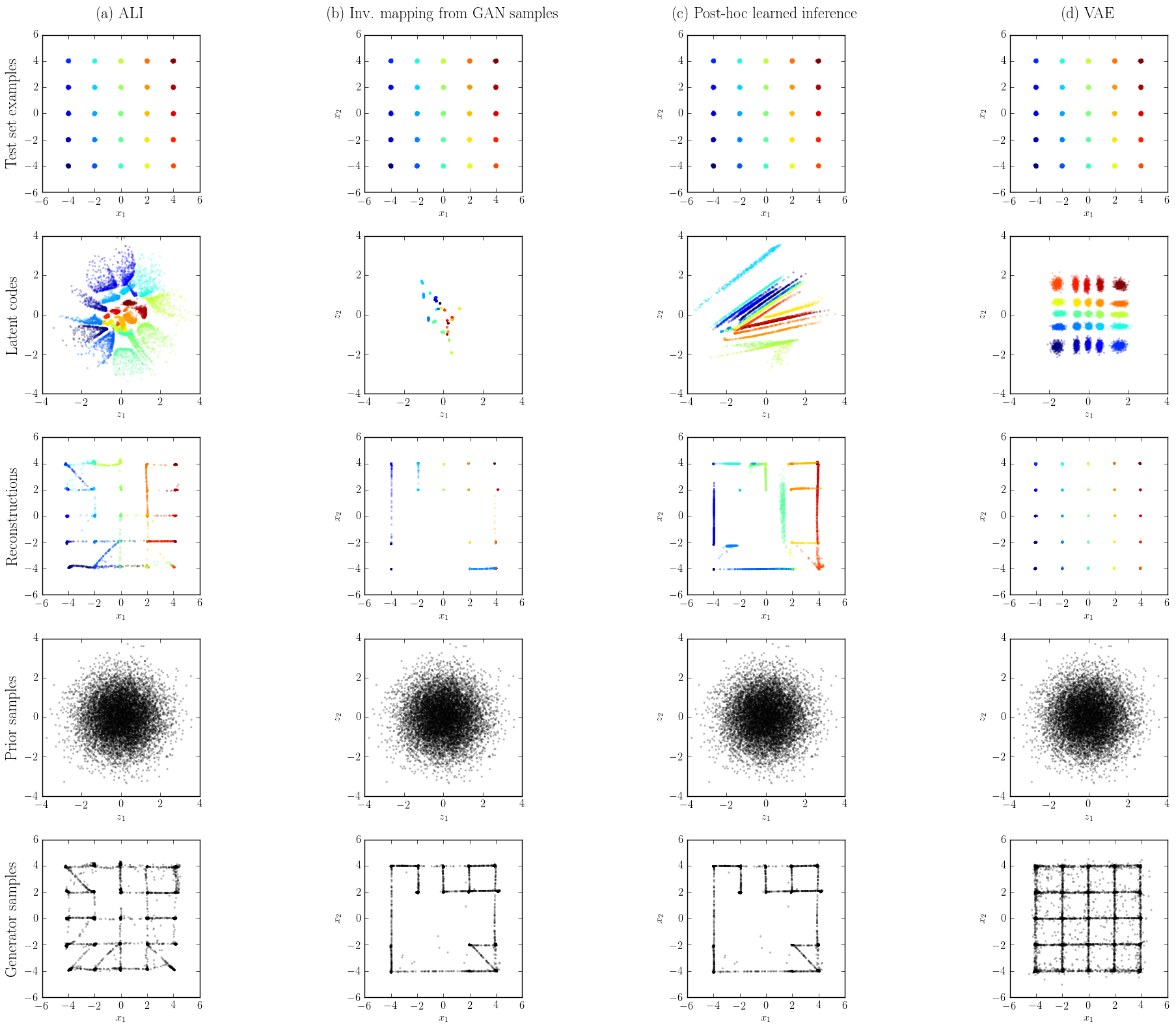
To highlight the role of the inference network during learning, we performed an experiment on a toy dataset for which $q(\bm{x})$ is a 2D gaussian mixture with 25 mixture components laid out on a grid. The covariance matrices and centroids have been chosen such that the distribution exhibits lots of modes separated by large low-probability regions, which makes it a decently hard task despite the 2D nature of the dataset.

We trained ALI and GAN on 100,000 $q(\bm{x})$ samples. The decoder and discriminator architectures are identical between ALI and GAN (except for the input of the discriminator, which receives the concatenation of $\bf{x}$ and $\bf{z}$ in the ALI case). Each model was trained 10 times using Adam (Kingma & Ba, 2014) with random learning rate and $\beta_{1}$ values, and the weights were initialized by drawing from a gaussian distribution with a random standard deviation.

We measured the extent to which the trained models covered all 25 modes by drawing 10,000 samples from their $p(\bm{x})$ distribution and assigning each sample to a $q(\bm{x}$) mixture component according to the mixture responsibilities. We defined a dropped mode as one that wasn’t assigned to any sample. Using this definition, we found that ALI models covered $13.4\pm 5.8$ modes on average (min: 8, max: 25) while GAN models covered $10.4\pm 9.2$ modes on average (min: 1, max: 22).

We then selected the best-covering ALI and GAN models, and the GAN model was augmented with an encoder using the learned inverse mapping and post-hoc learned inference procedures outlined in subsection 2.2. The encoders learned for GAN inference have the same architecture as ALI’s encoder. We also trained a VAE with the same encoder-decoder architecture as ALI to outline the qualitative differences between ALI and VAE models.

We then compared each model’s inference capabilities by reconstructing 10,000 held-out samples from $q(\bm{x})$. Figure 8 summarizes the experiment. We observe the following:

• The ALI encoder models a marginal distribution $q(\bm{z})$ that matches $\bm{p(z)}$ fairly well (row 2, column a). The learned representation does a decent job at clustering and organizing the different mixture components.

• The GAN generator (row 5, columns b-c) has more trouble reaching all the modes than the ALI generator (row 5, column a), even over 10 runs of hyperparameter search.

• Learning an inverse mapping from GAN samples does not work very well: the encoder has trouble covering the prior marginally and the way it clusters mixture components is not very well organized (row 2, column b). As discussed in subsection 2.2, reconstructions suffer from the generator dropping modes.

• Learning inference post-hoc doesn’t work as well as training the encoder and the decoder jointly. As had been hinted at in subsection 2.2, it appears that adversarial training benefits from learning inference at training time in terms of mode coverage. This also negatively impacts how the latent space is organized (row 2, column c). However, it appears to be better at matching $q(\bm{z})$ and $p(\bm{z})$ than when inference is learned through inverse mapping from GAN samples.

• Due to the nature of the loss function being optimized, the VAE model covers all modes easily (row 5, column d) and excels at reconstructing data samples (row 3, column d). However, they have a much more pronounced tendency to smear out their probability density (row 5, column d) and leave “holes” in $\bf{q(z)}$ (row 2, column d). Note however that recent approaches such as Inverse Autoregressive Flow (Kingma et al., 2016) may be used to improve on this, at the cost of a more complex mathematical framework.

In summary, this experiment provides evidence that adversarial training benefits from learning an inference mechanism jointly with the decoder. Furthermore, it shows that our proposed approach for learning inference in an adversarial setting is superior to the other approaches investigated.

5 Conclusion

We introduced the adversarially learned inference (ALI) model, which jointly learns a generation network and an inference network using an adversarial process. The model learns mutually coherent inference and generation networks, as exhibited by its reconstructions. The induced latent variable mapping is shown to be useful, achieving results competitive with the state-of-the-art on the semi-supervised SVHN and CIFAR10 tasks.

Acknowledgments

The authors would like to acknowledge the support of the following agencies for research funding and computing support: NSERC, Calcul Québec, Compute Canada. We would also like to thank the developers of Theano (Bergstra et al., 2010; Bastien et al., 2012; Theano Development Team, 2016), Blocks and Fuel (van Merriënboer et al., 2015), which were used extensively for the paper. Finally, we would like to thank Yoshua Bengio, David Warde-Farley, Yaroslav Ganin and Laurent Dinh for their valuable feedback.

Appendix A Hyperparameters

Operation	Kernel	Strides	Feature maps	BN?	Dropout	Nonlinearity
$G_{z}(x)$ – $3\times 32\times 32$ input
Convolution	$5\times 5$	$1\times 1$	$32$	$\surd$	0.0	Leaky ReLU
Convolution	$4\times 4$	$2\times 2$	$64$	$\surd$	0.0	Leaky ReLU
Convolution	$4\times 4$	$1\times 1$	$128$	$\surd$	0.0	Leaky ReLU
Convolution	$4\times 4$	$2\times 2$	$256$	$\surd$	0.0	Leaky ReLU
Convolution	$4\times 4$	$1\times 1$	$512$	$\surd$	0.0	Leaky ReLU
Convolution	$1\times 1$	$1\times 1$	$512$	$\surd$	0.0	Leaky ReLU
Convolution	$1\times 1$	$1\times 1$	$128$	$\times$	0.0	Linear
$G_{x}(z)$ – $64\times 1\times 1$ input
Transposed convolution	$4\times 4$	$1\times 1$	$256$	$\surd$	0.0	Leaky ReLU
Transposed convolution	$4\times 4$	$2\times 2$	$128$	$\surd$	0.0	Leaky ReLU
Transposed convolution	$4\times 4$	$1\times 1$	$64$	$\surd$	0.0	Leaky ReLU
Transposed convolution	$4\times 4$	$2\times 2$	$32$	$\surd$	0.0	Leaky ReLU
Transposed convolution	$5\times 5$	$1\times 1$	$32$	$\surd$	0.0	Leaky ReLU
Convolution	$1\times 1$	$1\times 1$	$32$	$\surd$	0.0	Leaky ReLU
Convolution	$1\times 1$	$1\times 1$	$3$	$\times$	0.0	Sigmoid
$D(x)$ – $3\times 32\times 32$ input
Convolution	$5\times 5$	$1\times 1$	$32$	$\times$	0.2	Maxout
Convolution	$4\times 4$	$2\times 2$	$64$	$\times$	0.5	Maxout
Convolution	$4\times 4$	$1\times 1$	$128$	$\times$	0.5	Maxout
Convolution	$4\times 4$	$2\times 2$	$256$	$\times$	0.5	Maxout
Convolution	$4\times 4$	$1\times 1$	$512$	$\times$	0.5	Maxout
$D(z)$ – $64\times 1\times 1$ input
Convolution	$1\times 1$	$1\times 1$	$512$	$\times$	0.2	Maxout
Convolution	$1\times 1$	$1\times 1$	$512$	$\times$	0.5	Maxout
$D(x,z)$ – $1024\times 1\times 1$ input
Concatenate $D(x)$ and $D(z)$ along the channel axis
Convolution	$1\times 1$	$1\times 1$	$1024$	$\times$	0.5	Maxout
Convolution	$1\times 1$	$1\times 1$	$1024$	$\times$	0.5	Maxout
Convolution	$1\times 1$	$1\times 1$	$1$	$\times$	0.5	Sigmoid
Optimizer	Adam ($\alpha=10^{-4}$, $\beta_{1}=0.5$, $\beta_{2}=10^{-3}$)
Batch size	100
Epochs	6475
Leaky ReLU slope, maxout pieces	0.1, 2
Weight, bias initialization	Isotropic gaussian ($\mu=0$, $\sigma=0.01$), Constant($0$)

Table 3: CIFAR10 model hyperparameters (unsupervised). Maxout layers (Goodfellow et al., 2013) are used in the discriminator.

Operation	Kernel	Strides	Feature maps	BN?	Dropout	Nonlinearity
$G_{z}(x)$ – $3\times 32\times 32$ input
Convolution	$5\times 5$	$1\times 1$	$32$	$\surd$	0.0	Leaky ReLU
Convolution	$4\times 4$	$2\times 2$	$64$	$\surd$	0.0	Leaky ReLU
Convolution	$4\times 4$	$1\times 1$	$128$	$\surd$	0.0	Leaky ReLU
Convolution	$4\times 4$	$2\times 2$	$256$	$\surd$	0.0	Leaky ReLU
Convolution	$4\times 4$	$1\times 1$	$512$	$\surd$	0.0	Leaky ReLU
Convolution	$1\times 1$	$1\times 1$	$512$	$\surd$	0.0	Leaky ReLU
Convolution	$1\times 1$	$1\times 1$	$512$	$\times$	0.0	Linear
$G_{x}(z)$ – $256\times 1\times 1$ input
Transposed convolution	$4\times 4$	$1\times 1$	$256$	$\surd$	0.0	Leaky ReLU
Transposed convolution	$4\times 4$	$2\times 2$	$128$	$\surd$	0.0	Leaky ReLU
Transposed convolution	$4\times 4$	$1\times 1$	$64$	$\surd$	0.0	Leaky ReLU
Transposed convolution	$4\times 4$	$2\times 2$	$32$	$\surd$	0.0	Leaky ReLU
Transposed convolution	$5\times 5$	$1\times 1$	$32$	$\surd$	0.0	Leaky ReLU
Convolution	$1\times 1$	$1\times 1$	$32$	$\surd$	0.0	Leaky ReLU
Convolution	$1\times 1$	$1\times 1$	$3$	$\times$	0.0	Sigmoid
$D(x)$ – $3\times 32\times 32$ input
Convolution	$5\times 5$	$1\times 1$	$32$	$\times$	0.2	Leaky ReLU
Convolution	$4\times 4$	$2\times 2$	$64$	$\surd$	0.2	Leaky ReLU
Convolution	$4\times 4$	$1\times 1$	$128$	$\surd$	0.2	Leaky ReLU
Convolution	$4\times 4$	$2\times 2$	$256$	$\surd$	0.2	Leaky ReLU
Convolution	$4\times 4$	$1\times 1$	$512$	$\surd$	0.2	Leaky ReLU
$D(z)$ – $256\times 1\times 1$ input
Convolution	$1\times 1$	$1\times 1$	$512$	$\times$	0.2	Leaky ReLU
Convolution	$1\times 1$	$1\times 1$	$512$	$\times$	0.2	Leaky ReLU
$D(x,z)$ – $1024\times 1\times 1$ input
Concatenate $D(x)$ and $D(z)$ along the channel axis
Convolution	$1\times 1$	$1\times 1$	$1024$	$\times$	0.2	Leaky ReLU
Convolution	$1\times 1$	$1\times 1$	$1024$	$\times$	0.2	Leaky ReLU
Convolution	$1\times 1$	$1\times 1$	$1$	$\times$	0.2	Sigmoid
Optimizer	Adam ($\alpha=10^{-4}$, $\beta_{1}=0.5$, $\beta_{2}=10^{-3}$)
Batch size	100
Epochs	100
Leaky ReLU slope	0.01
Weight, bias initialization	Isotropic gaussian ($\mu=0$, $\sigma=0.01$), Constant($0$)

Table 4: SVHN model hyperparameters (unsupervised).

Operation	Kernel	Strides	Feature maps	BN?	Dropout	Nonlinearity
$G_{z}(x)$ – $3\times 64\times 64$ input
Convolution	$2\times 2$	$1\times 1$	$64$	$\surd$	0.0	Leaky ReLU
Convolution	$7\times 7$	$2\times 2$	$128$	$\surd$	0.0	Leaky ReLU
Convolution	$5\times 5$	$2\times 2$	$256$	$\surd$	0.0	Leaky ReLU
Convolution	$7\times 7$	$2\times 2$	$256$	$\surd$	0.0	Leaky ReLU
Convolution	$4\times 4$	$1\times 1$	$512$	$\surd$	0.0	Leaky ReLU
Convolution	$1\times 1$	$1\times 1$	$512$	$\times$	0.0	Linear
$G_{x}(z)$ – $512\times 1\times 1$ input
Transposed convolution	$4\times 4$	$1\times 1$	$512$	$\surd$	0.0	Leaky ReLU
Transposed convolution	$7\times 7$	$2\times 2$	$256$	$\surd$	0.0	Leaky ReLU
Transposed convolution	$5\times 5$	$2\times 2$	$256$	$\surd$	0.0	Leaky ReLU
Transposed convolution	$7\times 7$	$2\times 2$	$128$	$\surd$	0.0	Leaky ReLU
Transposed convolution	$2\times 2$	$1\times 1$	$64$	$\surd$	0.0	Leaky ReLU
Convolution	$1\times 1$	$1\times 1$	$3$	$\times$	0.0	Sigmoid
$D(x)$ – $3\times 64\times 64$ input
Convolution	$2\times 2$	$1\times 1$	$64$	$\surd$	0.0	Leaky ReLU
Convolution	$7\times 7$	$2\times 2$	$128$	$\surd$	0.0	Leaky ReLU
Convolution	$5\times 5$	$2\times 2$	$256$	$\surd$	0.0	Leaky ReLU
Convolution	$7\times 7$	$2\times 2$	$256$	$\surd$	0.0	Leaky ReLU
Convolution	$4\times 4$	$1\times 1$	$512$	$\surd$	0.0	Leaky ReLU
$D(z)$ – $512\times 1\times 1$ input
Convolution	$1\times 1$	$1\times 1$	$1024$	$\times$	0.2	Leaky ReLU
Convolution	$1\times 1$	$1\times 1$	$1024$	$\times$	0.2	Leaky ReLU
$D(x,z)$ – $1024\times 1\times 1$ input
Concatenate $D(x)$ and $D(z)$ along the channel axis
Convolution	$1\times 1$	$1\times 1$	$2048$	$\times$	0.2	Leaky ReLU
Convolution	$1\times 1$	$1\times 1$	$2048$	$\times$	0.2	Leaky ReLU
Convolution	$1\times 1$	$1\times 1$	$1$	$\times$	0.2	Sigmoid
Optimizer	Adam ($\alpha=10^{-4}$, $\beta_{1}=0.5$)
Batch size	100
Epochs	123
Leaky ReLU slope	0.02
Weight, bias initialization	Isotropic gaussian ($\mu=0$, $\sigma=0.01$), Constant($0$)

Table 5: CelebA model hyperparameters (unsupervised).

Operation	Kernel	Strides	Feature maps	BN?	Dropout	Nonlinearity
$G_{z}(x)$ – $3\times 64\times 64$ input
Convolution	$4\times 4$	$2\times 2$	$64$	$\surd$	0.0	Leaky ReLU
Convolution	$4\times 4$	$1\times 1$	$64$	$\surd$	0.0	Leaky ReLU
Convolution	$4\times 4$	$2\times 2$	$128$	$\surd$	0.0	Leaky ReLU
Convolution	$4\times 4$	$1\times 1$	$128$	$\surd$	0.0	Leaky ReLU
Convolution	$4\times 4$	$2\times 2$	$256$	$\surd$	0.0	Leaky ReLU
Convolution	$4\times 4$	$1\times 1$	$256$	$\surd$	0.0	Leaky ReLU
Convolution	$1\times 1$	$1\times 1$	$2048$	$\surd$	0.0	Leaky ReLU
Convolution	$1\times 1$	$1\times 1$	$2048$	$\surd$	0.0	Leaky ReLU
Convolution	$1\times 1$	$1\times 1$	$512$	$\times$	0.0	Linear
$G_{x}(z)$ – $256\times 1\times 1$ input
Convolution	$1\times 1$	$1\times 1$	$2048$	$\surd$	0.0	Leaky ReLU
Convolution	$1\times 1$	$1\times 1$	$256$	$\surd$	0.0	Leaky ReLU
Transposed convolution	$4\times 4$	$1\times 1$	$256$	$\surd$	0.0	Leaky ReLU
Transposed convolution	$4\times 4$	$2\times 2$	$128$	$\surd$	0.0	Leaky ReLU
Transposed convolution	$4\times 4$	$1\times 1$	$128$	$\surd$	0.0	Leaky ReLU
Transposed convolution	$4\times 4$	$2\times 2$	$64$	$\surd$	0.0	Leaky ReLU
Transposed convolution	$4\times 4$	$1\times 1$	$64$	$\surd$	0.0	Leaky ReLU
Transposed convolution	$4\times 4$	$2\times 2$	$64$	$\surd$	0.0	Leaky ReLU
Convolution	$1\times 1$	$1\times 1$	$3$	$\times$	0.0	Sigmoid
$D(x)$ – $3\times 64\times 64$ input
Convolution	$4\times 4$	$2\times 2$	$64$	$\times$	0.2	Leaky ReLU
Convolution	$4\times 4$	$1\times 1$	$64$	$\surd$	0.2	Leaky ReLU
Convolution	$4\times 4$	$2\times 2$	$128$	$\surd$	0.2	Leaky ReLU
Convolution	$4\times 4$	$1\times 1$	$128$	$\surd$	0.2	Leaky ReLU
Convolution	$4\times 4$	$2\times 2$	$256$	$\surd$	0.2	Leaky ReLU
Convolution	$4\times 4$	$1\times 1$	$256$	$\surd$	0.2	Leaky ReLU
$D(z)$ – $256\times 1\times 1$ input
Convolution	$1\times 1$	$1\times 1$	$2048$	$\times$	0.2	Leaky ReLU
Convolution	$1\times 1$	$1\times 1$	$2048$	$\times$	0.2	Leaky ReLU
$D(x,z)$ – $2304\times 1\times 1$ input
Concatenate $D(x)$ and $D(z)$ along the channel axis
Convolution	$1\times 1$	$1\times 1$	$4096$	$\times$	0.2	Leaky ReLU
Convolution	$1\times 1$	$1\times 1$	$4096$	$\times$	0.2	Leaky ReLU
Convolution	$1\times 1$	$1\times 1$	$1$	$\times$	0.2	Sigmoid
Optimizer	Adam ($\alpha=10^{-4}$, $\beta_{1}=0.5$, $\beta_{2}=10^{-3}$)
Batch size	128
Epochs	125
Leaky ReLU slope	0.01
Weight, bias initialization	Isotropic gaussian ($\mu=0$, $\sigma=0.01$), Constant($0$)

Table 6: Tiny ImageNet model hyperparameters (unsupervised).

Appendix B A generative story for ALI

Figure 9: A Circle of Infinite Painters’ view of the ALI game.

The Circle of Infinite Painters is a very prolific artistic group. Very little is known about the Circle, but what we do know is that it is composed of two very brilliant artists. It has produced new paintings almost daily for more than twenty years, each one more beautiful than the others. Not only are the paintings exquisite, but their title and description is by itself a literary masterpiece.

However, some scholars believe that things might not be as they appear: certain discrepancies in the Circle’s body of work hints at the Circle being composed of more than one artistic duo. This is what Joseph Discriminator, art critique and world expert on the Circle, believes. He’s recently been working intensively on the subject. Without knowing it, he’s right: the Circle is not one, but two artistic duos.

Xavier and Zach Prior form the creative component of the group. Xavier is a painter and can, in one hour and starting from nothing, produce a painting that would make any great painter jealous. Impossible however for him to explain what he’s done: he works by intuition alone. Zach is an author and his literary talent equals Xavier’s artistic talent. His verb is such that the scenes he describes could just as well be real.

By themselves, the Prior brothers cannot collaborate: Xavier can’t paint anything from a description and Zach is bored to death with the idea of describing anything that does not come out of his head. This is why the Prior brothers depend on the Conditional sisters so much.

Zelda Conditional has an innate descriptive talent: she can examine a painting and describe it so well that the original would seem like an imitation. Xena Conditional has a technical mastery of painting that allows her to recreate everything that’s described to her in the most minute details. However, their creativity is inversely proportional to their talent: by themselves, they cannot produce anything of interest.

As such, the four members of the Circle work in pairs. What Xavier paints, Zelda describes, and what Zach describes, Xena paints. They all work together to fulfill the same vision of a unified Circle of Infinite Painters, a whole greater than the sum of its parts.

This is why Joseph Discriminator’s observations bother them so much. Secretly, the Circle put Mr. Discriminator under surveillance. Whatever new observation he’s made, they know right away and work on attenuating the differences to maintain the illusion of a Circle of Infinite Painters made of a single artistic duo.

Will the Circle reach this ideal, or will it be unmasked by Mr. Discriminator?

References

- Bastien et al. (2012) Frédéric Bastien, Pascal Lamblin, Razvan Pascanu, James Bergstra, Ian Goodfellow, Arnaud Bergeron, Nicolas Bouchard, David Warde-Farley, and Yoshua Bengio. Theano: new features and speed improvements. arXiv preprint arXiv:1211.5590, 2012.
- Bengio et al. (2013a) Yoshua Bengio, Nicholas Léonard, and Aaron Courville. Estimating or propagating gradients through stochastic neurons for conditional computation. arXiv preprint arXiv:1308.3432, 2013a.
- Bengio et al. (2013b) Yoshua Bengio, Eric Thibodeau-Laufer, Guillaume Alain, and Jason Yosinski. Deep generative stochastic networks trainable by backprop. arXiv preprint arXiv:1306.1091, 2013b.
- Bergstra et al. (2010) James Bergstra, Olivier Breuleux, Frédéric Bastien, Pascal Lamblin, Razvan Pascanu, Guillaume Desjardins, Joseph Turian, David Warde-Farley, and Yoshua Bengio. Theano: a cpu and gpu math expression compiler. In Proceedings of the Python for scientific computing conference (SciPy), volume 4, pp. 3. Austin, TX, 2010.
- Brock et al. (2016) Andrew Brock, Theodore Lim, JM Ritchie, and Nick Weston. Neural photo editing with introspective adversarial networks. arXiv preprint arXiv:1609.07093, 2016.
- Chen et al. (2016) Xi Chen, Yan Duan, Rein Houthooft, John Schulman, Ilya Sutskever, and Pieter Abbeel. Infogan: Interpretable representation learning by information maximizing generative adversarial nets. In Advances in Neural Information Processing Systems, pp. 2172–2180, 2016.
- Donahue et al. (2016) Jeff Donahue, Philipp Krähenbühl, and Trevor Darrell. Adversarial feature learning. arXiv preprint arXiv:1605.09782, 2016.
- Dosovitskiy & Brox (2016) Alexey Dosovitskiy and Thomas Brox. Generating images with perceptual similarity metrics based on deep networks. arXiv preprint arXiv:1602.02644, 2016.
- Dumoulin & Visin (2016) Vincent Dumoulin and Francesco Visin. A guide to convolution arithmetic for deep learning. arXiv preprint arXiv:1603.07285, 2016.
- Goodfellow et al. (2014) Ian Goodfellow, Jean Pouget-Abadie, Mehdi Mirza, Bing Xu, David Warde-Farley, Sherjil Ozair, Aaron Courville, and Yoshua Bengio. Generative adversarial nets. In Advances in Neural Information Processing Systems, pp. 2672–2680, 2014.
- Goodfellow et al. (2013) Ian J Goodfellow, David Warde-Farley, Mehdi Mirza, Aaron Courville, and Yoshua Bengio. Maxout networks. arXiv preprint arXiv:1302.4389, 2013.
- Kingma & Ba (2014) Diederik Kingma and Jimmy Ba. Adam: A method for stochastic optimization. arXiv preprint arXiv:1412.6980, 2014.
- Kingma (2013) Diederik P Kingma. Fast gradient-based inference with continuous latent variable models in auxiliary form. arXiv preprint arXiv:1306.0733, 2013.
- Kingma & Welling (2013) Diederik P Kingma and Max Welling. Auto-encoding variational bayes. arXiv preprint arXiv:1312.6114, 2013.
- Kingma et al. (2014) Diederik P Kingma, Shakir Mohamed, Danilo Jimenez Rezende, and Max Welling. Semi-supervised learning with deep generative models. In Advances in Neural Information Processing Systems, pp. 3581–3589, 2014.
- Kingma et al. (2016) Diederik P Kingma, Tim Salimans, and Max Welling. Improving variational inference with inverse autoregressive flow. arXiv preprint arXiv:1606.04934, 2016.
- Krizhevsky & Hinton (2009) Alex Krizhevsky and Geoffrey Hinton. Learning multiple layers of features from tiny images, 2009.
- Lamb et al. (2016) Alex Lamb, Vincent Dumoulin, and Aaron Courville. Discriminative regularization for generative models. arXiv preprint arXiv:1602.03220, 2016.
- Larsen et al. (2015) Anders Boesen Lindbo Larsen, Søren Kaae Sønderby, and Ole Winther. Autoencoding beyond pixels using a learned similarity metric. arXiv preprint arXiv:1512.09300, 2015.
- Lin (1991) Jianhua Lin. Divergence measures based on the shannon entropy. Information Theory, IEEE Transactions on, 37(1):145–151, 1991.
- Liu et al. (2015) Ziwei Liu, Ping Luo, Xiaogang Wang, and Xiaoou Tang. Deep learning face attributes in the wild. In Proceedings of the IEEE International Conference on Computer Vision, pp. 3730–3738, 2015.
- Maaløe et al. (2016) Lars Maaløe, Casper Kaae Sønderby, Søren Kaae Sønderby, and Ole Winther. Auxiliary deep generative models. arXiv preprint arXiv:1602.05473, 2016.
- Makhzani et al. (2015) Alireza Makhzani, Jonathon Shlens, Navdeep Jaitly, and Ian Goodfellow. Adversarial autoencoders. arXiv preprint arXiv:1511.05644, 2015.
- Netzer et al. (2011) Yuval Netzer, Tao Wang, Adam Coates, Alessandro Bissacco, Bo Wu, and Andrew Y Ng. Reading digits in natural images with unsupervised feature learning. In NIPS workshop on deep learning and unsupervised feature learning, volume 2011, pp. 4. Granada, Spain, 2011.
- Odena et al. (2016) Augustus Odena, Vincent Dumoulin, and Chris Olah. Deconvolution and checkerboard artifacts. http://distill.pub/2016/deconv-checkerboard/, 2016.
- Radford et al. (2015) Alec Radford, Luke Metz, and Soumith Chintala. Unsupervised representation learning with deep convolutional generative adversarial networks. arXiv preprint arXiv:1511.06434, 2015.
- Rasmus et al. (2015) Antti Rasmus, Harri Valpola, Mikko Honkala, Mathias Berglund, and Tapani Raiko. Semi-supervised learning with ladder network. In Advances in Neural Information Processing Systems, 2015, 2015.
- Rezende et al. (2014) Danilo Jimenez Rezende, Shakir Mohamed, and Daan Wierstra. Stochastic backpropagation and approximate inference in deep generative models. arXiv preprint arXiv:1401.4082, 2014.
- Russakovsky et al. (2015) Olga Russakovsky, Jia Deng, Hao Su, Jonathan Krause, Sanjeev Satheesh, Sean Ma, Zhiheng Huang, Andrej Karpathy, Aditya Khosla, Michael Bernstein, et al. Imagenet large scale visual recognition challenge. International Journal of Computer Vision, 115(3):211–252, 2015.
- Salimans et al. (2016) Tim Salimans, Ian J. Goodfellow, Wojciech Zaremba, Vicki Cheung, Alec Radford, and Xi Chen. Improved techniques for training gans. arXiv preprint arXiv:1606.03498, 2016.
- Shi et al. (2016) Wenzhe Shi, Jose Caballero, Lucas Theis, Ferenc Huszar, Andrew Aitken, Christian Ledig, and Zehan Wang. Is the deconvolution layer the same as a convolutional layer? arXiv preprint arXiv:1609.07009, 2016.
- Springenberg (2015) Jost Tobias Springenberg. Unsupervised and semi-supervised learning with categorical generative adversarial networks. arXiv preprint arXiv:1511.06390, 2015.
- Theano Development Team (2016) Theano Development Team. Theano: A Python framework for fast computation of mathematical expressions. arXiv preprint arXiv:1605.02688, 2016.
- Theis et al. (2015) Lucas Theis, Aron van den Oord, and Matthias Bethge. A note on the evaluation of generative models. arXiv preprint arXiv:1511.01844, 2015.
- van den Oord et al. (2016a) Aaron van den Oord, Sander Dieleman, Heiga Zen, Karen Simonyan, Oriol Vinyals, Alex Graves, Nal Kalchbrenner, Andrew W. Senior, and Koray Kavukcuoglu. Wavenet: A generative model for raw audio. arXiv preprint arXiv:1609.03499, 2016a.
- van den Oord et al. (2016b) Aaron van den Oord, Nal Kalchbrenner, and Koray Kavukcuoglu. Pixel recurrent neural networks. arXiv preprint arXiv:1601.06759, 2016b.
- van den Oord et al. (2016c) Aaron van den Oord, Nal Kalchbrenner, Oriol Vinyals, Lasse Espeholt, Alex Graves, and Koray Kavukcuoglu. Conditional image generation with pixelcnn decoders. arXiv preprint arXiv:1606.05328, 2016c.
- van Merriënboer et al. (2015) Bart van Merriënboer, Dzmitry Bahdanau, Vincent Dumoulin, Dmitriy Serdyuk, David Warde-Farley, Jan Chorowski, and Yoshua Bengio. Blocks and fuel: Frameworks for deep learning. arXiv preprint arXiv:1506.00619, 2015.
- Zhao et al. (2015) Junbo Zhao, Michael Mathieu, Ross Goroshin, and Yann Lecun. Stacked what-where auto-encoders. arXiv preprint arXiv:1506.02351, 2015.