Rectangular Statistical Cartograms in R: The recmap Package

Christian Panse Compute the Rectangular Statistical Cartogram recmap: Compute the Rectangular Statistical Cartogram Cartogram drawing is a technique for showing geography-related statistical information, such as demographic and epidemiological data. The idea is to distort a map by resizing its regions according to a statistical parameter by keeping the map recognizable. This article describes an R package implementing an algorithm called RecMap which approximates every map region by a rectangle where the area corresponds to the given statistical value (maintain zero cartographic error). The package implements the computationally intensive tasks in C++. This paper’s contribution is that it demonstrates on real and synthetic maps how recmap can be used, how it is implemented and used with other statistical packages. cartogram, spatial data analysis, geovisualization, demographics, R cartogram, spatial data analysis, geovisualization, demographics, R 2016-06-01 Christian Panse
Functional Genomics Center Zurich UZH|ETHZ
Winterthurerstr. 190
CH-8057, Zürich, Switzerland
Telephone: +41/44/63-53912 E-mail:
URL: http://www.fgcz.ch/the-center/people/panse.html

1 Introduction

The idea to generate a cartogram is to distort a map by resizing its regions according to a given statistical parameter, but in a way that keeps the map recognizable. These so-called cartograms or value-by-area maps may be used to visualize any geo-spatial related data, e.g., political, economical, or public health data. There exists several algorithms to compute so-called contiguous cartograms. An overview on historic, hand-drawn, and computer generated cartograms can be found in Waldo; TheStateoftheArtInCartograms.

For using contiguous cartograms, the diffusion-based method of pmid15136719 is available through the R packages Rcartogram and getcartr Rcartogram; getcartr.

An alternative approach to contiguous cartograms is to entirely relax the map topology by approximating each map region by basic geometric objects like rectangles or circles (circle). Such rectangular cartograms can be generated from geolocation and statistical data. Hence, they provide a useful alternative, even if there are no boundaries available or some statistical values are missing. First rectangular cartograms were drawn by hand following a system of construction (ErwinRaisz). Recent research publication on rectangular cartogram drawing include Speckmann2004; Speckmann2007; Speckmann2012; Buchin:2016. However, according to a recent publication, both variants of recmap are the only rectangular cartogram algorithms that “maintain zero cartographic error” (TheStateoftheArtInCartograms, section 5.4).

The recmap package discussed in this article contains an implementation of the RecMap (Map Partition variant 2) algorithm recmap to draw maps according to given statistical parameter. A typical usage of a cartogram based visualization is demonstrated in Figure 1.

Figure 1: A rectangular statistical cartogram of the U.S. election in 2004 is drawn. The area corresponds to the number of electors. Color is indicating the outcome of the vote. Democrats are represented by the color blue and republicans are represented through red coloring. Regions with low saturation, e.g., Ohio, Pennsylvania, and Florida, mark states with a tight outcome of the vote (also known as swing states). The election cartogram was computed by using the original implementation of the construction heuristic RecMap MP2 introduced by recmap. map source: U.S. Census Bureau; election data source: http://www.electoral-vote.com/, November 2004.

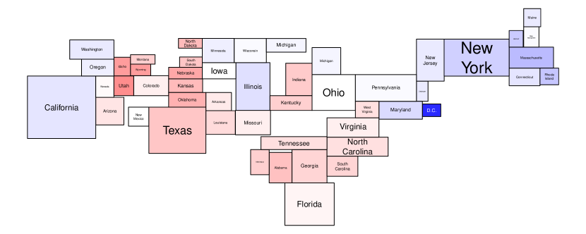
The article is organized as follows: The next section defines the input and output of the recmap algorithm and the objective functions. In Section 3, the usage of the recmap package using the R shell is demonstrated. Section 4 discusses major implementation details and provides some benchmark and performance studies. Section 5 describes how two metaheuristics can be used to find an optimized cartogram drawing. In Section LABEL:section:application, a number of applications are presented. Section LABEL:section:summary summarizes and discuss the approach.

2 Problem definition and objective functions

The input

consists of a map represented by overlapping rectangles $\mathcal{R}=(r_{1},\ldots,r_{n})$. Each map region $r_{j}$ contains:

• a tuple of $(x,y)$ values corresponding to the (longitude, latitude) position,

• a tuple of $(dx,dy)$ of expansion along (longitude, latitude),

• and a statistical value $z$.

The $(x,y)$ coordinates represent the center of the minimal bounding boxes (MBB). The coordinates of the MBB are derived by adding or subtracting the $(dx,dy)$ tuple accordingly. A tuple $(dx,dy)$ defines also the ratio of the corresponding map region. The statistical values $(z_{1},\ldots,z_{n})$ define the desired area of each map region.

The ordering $\Pi$ is an index vector taken from the permutation set $Perm(n)$.

The output

is a rectangular cartogram $\mathcal{\overline{R}}$ where the map regions are:

• non overlapping,

• connected,

• rectangles are placed parallel to the axes.

Furthermore, for each map region the following criteria have to be satisfied:

• the area is equal to the desired area derived from the as input given statistical value $z$,

• the ratio, $dy/dx$, is preserved.

The recmap construction heuristic is a function

$$f:\mathbb{R}^{n\times 2}\times\mathbb{R}_{>0}^{n\times 3}\times Perm(n) \rightarrow \mathbb{R}^{n\times 2}\times\mathbb{R}_{>0}^{n\times 2}$$ (1)

which transforms the set of input rectangles $\mathcal{R}$ and a permutation $\Pi$ into a rectangular cartogram

$$\overline{\mathcal{R}} = f(\mathcal{R},\Pi)$$ (2)

so that important spatial constraints, in particular

• the topology of the dual graph $G(\mathcal{R},E)$, defined by the overlapping input rectangles,

• the relative position of map region centers,

are tried to be preserved.

If the output satifies these criteria, the rectangular cartogram is denoted as feasible solution.

The following equation were introduced by cartodraw. The desired area $\tilde{A_{j}}$ of a map region $r_{j}$ is defined as

$$\tilde{A_{j}} = z_{j}\cdot\frac{\sum_{i=1}^{n}A(r_{i})}{\sum_{i=1}^{n}z_{i}}$$ (3)

where the area of the rectangle $r$ is defined by

$$A(r) = 4\cdot dx\cdot dy$$ (4)

The objective functions for area $d_{A}$, shape $d_{S}$ (ratios of the MBBs), relative positon $d_{R}$, and map topology $d_{T}$, are as defined and described by recmap:

$$d_{A} = d_{A}(\mathcal{R,\overline{R}})$$ (5)

$$= \sum_{j=1}^{n}|A_{j}-\tilde{A_{j}}|$$ (6)

$$d_{S} = d_{S}(\mathcal{\mathcal{R},\overline{R}})$$ (7)

$$= \sum_{j=1}^{n}|(dy_{j}/dx_{j})-(\overline{dy_{j}}/\overline{dx_{j}})|$$ (8)

$$d_{T} = d_{T}(\mathcal{\mathcal{R},\overline{R}})$$ (9)

$$= \frac{|\overline{E}_{a}\backslash E_{a}|+|E_{a}\backslash\overline{E}_{a}|}{|\overline{E}_{a}\cup E_{a}|},$$ (10)

$$d_{R} = d_{R}(\mathcal{R},\mathcal{\overline{R}})$$ (11)

$$= \frac{2}{n\cdot\left(n-1\right)}\cdot\sum\limits_{i=1}^{n-1}\sum\limits_{j=i+1}^{n}|\measuredangle(\underbrace{r_{i},r_{j}}_{\in\mathcal{R}})-\measuredangle(\underbrace{\tilde{r_{i}},\tilde{r_{j}}}_{\in\mathcal{\overline{R}}})|$$ (12)

Note, if $\forall j\in\{1,\ldots,n\}:A_{j}=\tilde{A_{j}}\Rightarrow d_{A}=0$ and if $\forall j\in\{1,\ldots,n\}:dy_{j}/dx_{j}=\overline{dy_{j}}/\overline{dx_{j}}\Rightarrow d_{S}=0$. $n=|\mathcal{R}|$ and $E$ denotes the edges of the dual graph. $dT$ determines the differences in the pseudo dual graphs. $dR$ measures the angle differences between all pairs of rectangle centers of the input map and output cartogram by using $\measuredangle(x,y)$ defined as follows:

$$\measuredangle(x,y) = \arctan_{2}(x,y)$$ (13)

To find an optimal rectangular statistical cartogram out of all feasible solutions, as it will be intended in this manuscript using recmap, the optimization problem can be expressed as follows:

$$\underset{\Pi\in Perm(n)}{\text{minimize}} a\cdot d_{R}+b\cdot d_{T}\text{~{}with~{}}a,b\in\mathbb{R}_{\geq 0}$$ (14)

subject to $$d_{A}=0,d_{S}=0.$$ (15)

To find a sufficiently good solution for the optimization problem a metaheuristic, as described in section 5, will be applied.

Term	Description	Equation
$\mathcal{R}=(r_{1},\ldots,r_{n})$	overlapping input rectangles
$(x,y)$	coordinates represent the center of a rectangle
$(dx,dy)$	expansion along x and y axes
$z$	statistical value of a rectangle
$G(\mathcal{R},E)$	dual graph of $\mathcal{R}$
$\Pi$	permutation
$A(r)$	area of a rectangle
$\tilde{A_{j}}$	desired area of a map region $j$	3
$d_{A}$	area error	5
$d_{S}$	shape error	8
$d_{T}$	topology error	10
$d_{R}$	relative position error	12
$\measuredangle(x,y)$	angle between two points $x$ and $y$ in $\mathbb{R}^{2}$	13
$f$	construction heuristic	1
$\overline{\mathcal{R}}$	output / cartogram	2

Table 1: The table provides a glossary of the used algebraic terms.

3 The package usage

3.1 Input

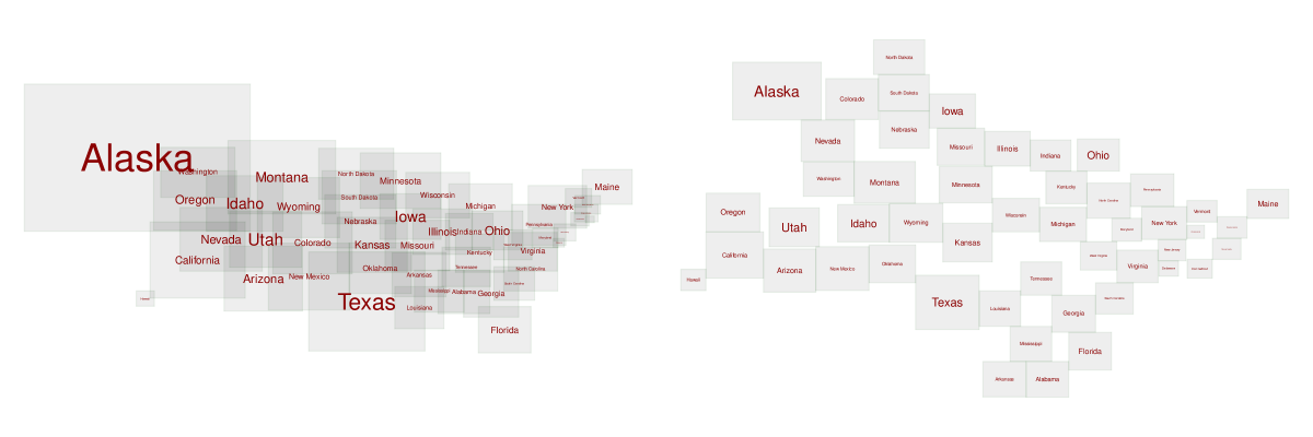
The U.S. map on state level is often used to compare cartogram algorithms. To generate a useful dual graph, which is a requirement of the algorithm, the input map regions have to overlap. For the state.x77 data used in this section this can be done by correcting lines of longitude derived by the square roots of the area values (see Figure 2 left).

R> US.map <- data.frame(x=state.center$x,+y=state.center$y, + dx = sqrt(state.area) / 2 / (0.7 * 60 * cos(state.center$y*pi/180)),+dy=sqrt(state.area)/2/(0.7*60),+z=sqrt(state.area),+name=state.name)R>head(US.map)\Soutput xydxdyzname1-86.750932.59013.2098902.704478227.1761Alabama2-127.250049.250014.0056709.142338767.9564Alaska3-111.625034.21924.8590444.017906337.5041Arizona4-92.299234.73363.3382042.743370230.4431Arkansas5-119.773036.53415.9021774.742415398.3629California6-105.513038.67774.9236023.843727322.8730Colorado\par Pleasenote,ingeneral\code{recmap}isnottransformingthegeodeticdatum,e.g.,WGS84orSwissgrid.Furthermore,geospatialpositionshavetobemappedfromtheearthsurfacetotheplane.Thishastobedonepriorthethecartogramgeneration.Anoverviewofmapprojectioncanbefoundin\cite[citet]{\@@bibref{Authors Phrase1YearPhrase2}{snyder1997flattening}{\@@citephrase{(}}{\@@citephrase{)}}}.Mapprojectionsaimtooptimizetowardsdifferentobjectives,e.g.,conformalmapping(preservationoflocalangles)orareamapping(preservationofarea).Incartogrampublicationsthemapprojectionaspectisoftenneglectedandconformalerrorsareaccepted.However,studyingU.S.cartograms,acylindricalprojectionseemstobetheprojectionofchoice.The\proglang{R}usercanfindsupportforawidevarietyofadequatemapprojectionsduetousingthe\pkg{mapproj}packageby\cite[cite]{\@@bibref{Authors Phrase1YearPhrase2}{mapproj}{\@@citephrase{(}}{\@@citephrase{)}}}.\par$

3.2 Run

The algorithm takes a data.frame object having the column names c(’x’, ’y’, ’dx’, ’dy’, ’z’, ’name’), here the US.map object, as input. Additional control is given by the index order and the (dx, dy) values. The index order $\Pi$ defines in which order the dual graph is explored and the (dx, dy) values define which map region are adjacent.

R> library("recmap") R> # Generate the rectangular statistical cartogram. R> US.cartogram <- recmap(US.map)

3.3 The output

The recmap method returns an S3 class object c(’recmap’, ’data.frame’) of the transformed map. Additional columns in the result contain information for topology and relative position error defined in Equations 10 and 12. The column dfn.num indicates in which order the dual graph has been explored.

R> head(US.cartogram) x y dx dy z name dfs.num 1 -79.27226 10.40598 3.916894 3.300161 227.1761 Alabama 23 2 -129.22283 63.71115 8.181797 5.340748 767.9564 Alaska 49 3 -126.86923 30.51915 4.819169 3.984933 337.5041 Arizona 34 4 -87.19357 10.42302 3.994415 3.282650 230.4431 Arkansas 39 5 -137.00972 33.40013 5.311325 4.267664 398.3629 California 35 6 -115.35010 62.23315 4.851078 3.787109 322.8730 Colorado 48 topology.error relpos.error relposnh.error 1 6 0.3917837 0.7848231 2 6 0.5901459 1.9059785 3 3 0.2447048 0.3498989 4 8 0.5624989 1.0728192 5 4 0.1861821 0.2596710 6 10 0.7576109 1.4491548

Input and output of the recmap function can be visualized using the S3 method plot.recmap. The output of the R code snippet can be seen in Figure 2. As default the plot.recmap function places the name attribute in the centre of each rectangle. To avoid overplotting of the labels, the text is scaled by using cex = dx / strwidth(name) as argument for the text function. However small statistical values result in small label areas. This problem can be circumvented by using an interactive visualization, e.g., using shiny the function hoverOpts enables the “mouseover” feature. Please note: while the input US.map is not classified as a recmap class, the plot.recmap function can not be dispatched by the S3 class system and has to be explicitly called.

R> op <- par(mfrow = c(1, 2), mar = c(0, 0, 0, 0)) R> plot.recmap(US.map, col.text = ’darkred’) R> plot(US.cartogram, col.text = ’darkred’)

A summary method implements the calculation of some meta data including the objective functions. R> summary(US.cartogram) values number of map regions 50.000000 area error 0.000000 topology error 266.000000 relative position error 0.420000 screen filling [in xmin -146.967409 xmax -34.722706 ymin 7.105818 ymax 73.190904

Figure 2: The “usage” example, generated from the “US State Facts and Figures” datasets package, was used for drawing a rectangular map approximation. The input set of overlapping rectangles is shown left. A feasible solution thereof generated with recmap is on the right side. The state area, original size of the map region, is used as statistical value.

4 Implementation

recmap is implemented in C++ using features provided by the C++-11 standard. The input and output data transfer between R and the C++ recmap class is handled by using the Rcpp (Rcpp) mechanism. The C++ recmap class itself consists of a std::vector of map_region. A map_region contains all the $(x,y,dx,dy,z)$ values, a std::vector of type int to it neighbor map regions, and some additional help variables to ease the error computation. In general the construction algorithm follows the map partition 2 (MP2) procedure described in recmap. The local placement function can place any rectangle next to another rectangle as it is demonstrated in Figure 3. The current implementation starts with the original bearing $\alpha$ of the two map region centers (see Figure 3 where $\beta=0$). If the placement does not lead to a feasible solution, the angle $\beta$ is added to $\alpha$. $\beta$ is iterating between $[0,\pi]$ with step size of $\frac{\pi}{180}$ and a changing sign until a placement without overlap has been found. If no placement can be found, the algorithm considers all adjacent placed map regions. If also in a later step during the DFS a map region can not be placed, a non feasible solution is accepted. This situation is often caused because the construction algorithm is hampered by the input configuration of the map regions. Solving this can be very compute expensive and often the procedure leads to a solution which will be rejected by the metaheuristic due to the bad fitness value.

Figure 3: The rainbow colored rectangles graph the feasable positions of a local placement function $f_{pl}$ to place a rectangle $B$ around a given rectangle $A$ of any angle $\alpha$ between $[-\pi,\pi]$ (left figure). There are special cases for quadrant I, II, III, and IV indicated by different colors in the graphic. On the right figure, B should be placed around A starting with an angle of $\frac{\pi}{4}$ (this is the initial relative position in the input map). Since the rectangle can not be placed without overlap (indicated by red) an angle $\beta$ is added.

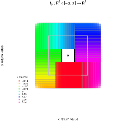
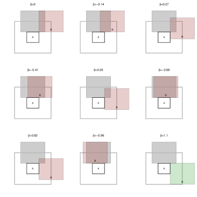
Furthermore, no genetic algorithm (metaheuristic) has been implemented. Here recmap will use the GA package available on CRAN as demonstrated in section 5. The most computationally expensive part is the computation of MBB intersections which has to be performed to achieve feasible solutions, multiple times, for each placement step. In the package version 0.2.1 these tests were performed by iterating over each map region. All later versions use a std::multiset data structure and a std::lower_bound algorithm of the C++ Standard Template Library (STL) to reduce the search space.

The time complexity for one recmap run is $\mathcal{O}(n^{2})$, where $n$ is the number of regions. A depth first search (DFS) run is visiting each map region only once and therefore it has time complexity $\mathcal{O}(n)$. For each map_region placement a constant number of MBB intersection are called (max 360). MBB check is implemented using std::multiset container, and the functions std::insert, std::upper_bound, and std::upper_bound. The time complexity for all of these functions are reported on http://www.cplusplus.com/reference/stl as $\mathcal{O}(\log(n))$. However, the worst case scenario for a range query is $\mathcal{O}(n)$, iff dx or dy cover the whole x or y range. The boxplots in Figure 4 (left plot) show that the number of MBB intersection test calls could be reduced by using a std::multiset data structure. For this benchmark, synthetic checkerboards with a number of map regions in the interval of $\left[2^{2},\ldots,20^{2}\right]$ were generated using the R function checkerboard. For each checkerboard size recmap was called 100 times using different index orderings of the checkerboard input. The index order of the input records have a direct impact how the DFS is traversing the map. This characteristic will later be used for the metaheuristic.

For a performance study the checkerboard bench described above was repeated using the rbenchmark package by rbenchmark to measure the proc.time. The study was performed on two systems (using one core only). An Intel(R) Core(TM) i5-2500 CPU @ 3.30GHz running a Debian 8 using a 3.16.0-4-amd64 Kernel and a 3 GHz Intel Core i7 (Apple MacBook Pro) running OS X 10.11.4 (15E65) using a Darwin 15.4.0 Kernel. The middle graphic in Figure 4 displays the resulting mean aggregated measured data of the two (hardware / OS) systems using the two different implementations of the MBB intersection test. Beside the fact that the Linux system can not benefit from the more efficient implementation of the MBB intersection test, the graphic (middle) shows even for an input size of $20^{2}=400$ map regions, a rectangular cartogram can be computed in less than a second.

Figure 4: The boxplot (left) graphs the number of MBB intersection test calls for a given checkerboard size. The graph in the middle displays the mean aggregated measured computation time. The scatterplot (right) displays how many rectangular cartograms can be generated within one second depending on the board size.

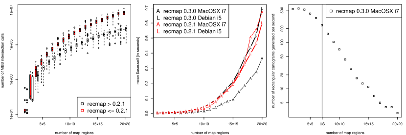
The right plot in Figure 4 was derived from the performance study (plot in the middle). It shows the number of rectangular cartograms which can be generated within one second depending on the number of map regions. The grey vertical line indicates the number of the U.S. map regions. The ability to generate a high number of cartogram candidates in a short time period is an important requirement for any metaheuristic as it is demonstrated in the next section.

5 Choose a metaheuristic

The design of the recmap algorithm is as follows: First, compute a set of feasible solutions. In a second evaluation step choose the best solution. In the current implementation, variations can be introduced by changing the index order $\Pi$ of the input data. This has a direct impact to the DFS traversal and leads to different cartogram layouts. The objective functions, equations 5 to 12, can be used to evaluate the result and to define a fitness function which has to be maximized. The following R code defines the fitness function which will be used as default.

R> recmap:::.recmap.fitness function (idxOrder, Map, …) Cartogram <- recmap(Map[idxOrder, ]) if (sum(Cartogram$topology.error==100)>0){return(0)}1/sum(Cartogram$relpos.error) <environment: namespace:recmap>

Other variants of fitness functions will lead to different results as it is shown in (recmap, Figure 4).

Since it is not possible to compute and evaluate all permutations, which is $n!$, random experiments are conducted. In the following section it is demonstrated how two metaheuristic, GRASP and GA, can be used to find a optimal layout for the rectangular statistical cartogram.

For a visual evaluation, of the in this section proposed metaheuristics, an 8x8 checkerboard will be used as input map. The map is generated using the checkerboard method R> Checkerboard <- checkerboard(8) R> summary(Checkerboard) values number of map regions 64.00 area error 0.27 topology error NA relative position error NA screen filling [in xmin 0.50 xmax 8.50 ymin 0.50 ymax 8.50 and can be seen in Figure LABEL:figure:cmp_GA_GRASP (left). If the assumption is made, that for each vertex, the cyclic order of edges in the contiguous cartogram remains the same as as in the input map, checkerboards provide examples of sets of map regions which do not have ideal cartogram solutions (cartodraw, Definition 2, Lemma 1, Fig. 3.).

5.1 Greedy Randomized Adaptive Search Procedures

One group of optimizer is “trivial to efficiently implement” (GRASP) and can directly benefit from a parallel environment is called greedy randomized adaptive search procedures (GRASP). The R method recmapGRASP defines a generic GRASP implementation as described in (GRASP, Fig. 1). The recmapGRASP function generates a set of rectangular cartograms which have different layouts caused by the random sampling. Each cartogram is evaluated. The best candidate is saved. The following command will generate cartogram solution based on a GRASP metaheuristic.

R> set.seed(1) R> res.GRASP <- recmapGRASP(Checkerboard) R> plot(res.GRASP$Cartogram,+col=c(^{\prime}white^{\prime},^{\prime}white^{\prime},^{\prime}white^{\prime},^{\prime}black^{\prime})[res.GRASP$Cartogram$z])\par AdrawingofthecartogramcanbefoundinFigure~{}\ref{figure:cmp_GA_GRASP}(middle).\par Forsometypesofinputmaps,GRASPcangenerateamazingresultsinashorttime.AsitcanbeseeninFigure~{}\ref{figure:cmp_GA_GRASP},forthecheckerboardmap,GRASPisoutperformedbythegeneticalgorithm,introducedinthenextsection.TheplotinFigure~{}\ref{figure:cmp_GA_GRASP2}(right)showsthatthesolutionprocessrunstoofastintoasaturation.\par$

5.2 Lessons learnt from biological evolution

In this paragraph a constraint-based genetic algorithm (GA) as discussed in recmap is used as metaheuristic. Here the construction heuristic benefits from the existence of the GA package by GA. The GA configuration used for recmap was directly derived from the traveling salesperson problem (TSP) example (GA, section 4.8) using the permutation type of the ga method. As genotype the index order $\Pi$ of the input map is used. The following command generates an almost perfect rectangular cartogram for the checkerboard map having 64 map regions on the author’s laptop within 60 seconds.

R> recmap.GA <- ga(type = "permutation", + fitness = recmap:::.recmap.fitness, + Map = Checkerboard, + min = 1, max = nrow(Checkerboard), + popSize = 64, + maxiter = 1000, + maxFitness = 1.7, + parallel = TRUE, + pmutation = 0.25)

The metaheuristic stops when a maximum number of iteration has been performed or the fitness value is higher than 1.7. Having reached a fitness value of 1.7 using the recmap.fitness function the result in Figure LABEL:figure:cmp_GA_GRASP (right) looks like an almost “optimal” solution.

The recmapGA function is a higher level wrapper function to glue the recmap construction heuristic with the metaheuristic ga.

R> res.GA <- recmapGA(Checkerboard) R> summary(res.GA) R> plot(res.GA$Cartogram,+col=c(^{\prime}white^{\prime},^{\prime}white^{\prime},^{\prime}white^{\prime},^{\prime}black^{\prime})[res.GA$Cartogram$z])\par The\code{recmapGA}functionreturnsalistoftheinput\code{Map},ThesolutionoftheGA,anda\code{recmap}objectcontainingthecartogram.TheresultingcartogramsusingaGAcanbeseeninFigure~{}\ref{figure:cmp_GA_GRASP}(right).TheredlineinFigure~{}\ref{figure:cmp_GA_GRASP2}(left)indicatesinwhichordertherectangleswereplacedusingtheDFSnumbering.Thered$∙$symbolmarksthefirstplacedrectangleandthe$⋄$thelastone.\text{Figure 5Figure 55Figure 55Acomparisonoftheinputmap,GR}$