Graph-Guided Banding of the Covariance Matrix
Abstract
Regularization has become a primary tool for developing reliable estimators of the covariance matrix in high-dimensional settings. To curb the curse of dimensionality, numerous methods assume that the population covariance (or inverse covariance) matrix is sparse, while making no particular structural assumptions on the desired pattern of sparsity. A highly-related, yet complementary, literature studies the specific setting in which the measured variables have a known ordering, in which case a banded population matrix is often assumed. While the banded approach is conceptually and computationally easier than asking for “patternless sparsity,” it is only applicable in very specific situations (such as when data are measured over time or one-dimensional space). This work proposes a generalization of the notion of bandedness that greatly expands the range of problems in which banded estimators apply.
We develop convex regularizers occupying the broad middle ground between the former approach of “patternless sparsity” and the latter reliance on having a known ordering. Our framework defines bandedness with respect to a known graph on the measured variables. Such a graph is available in diverse situations, and we provide a theoretical, computational, and applied treatment of two new estimators. An R package, called ggb, implements these new methods.
Keywords: covariance estimation, high-dimensional, hierarchical group lasso, network
1 Introduction
Understanding the relationships among large numbers of variables is a goal shared across many scientific areas. Estimating the covariance matrix is perhaps the most basic step toward understanding these relationships, and yet even this task is far from simple when sample sizes are small relative to the number of parameters to be estimated. High-dimensional covariance estimation is therefore an active area of research. Papers in this literature generally describe a set of structural assumptions that effectively reduces the dimension of the parameter space to make reliable estimation tractable given the available sample size. Some papers focus on eigenvalue-related structures and shrinkage (e.g., Johnstone 2001, Fan et al. 2008, Won et al. 2013, Donoho et al. 2013, Ledoit & Wolf 2004, among many others); others assume that correlations are constant or blockwise constant (such as in random effects models); and a very large number of papers introduce sparsity assumptions on the covariance matrix (or its inverse). Still other papers suggest combinations of these structures (Chandrasekaran et al. 2010, Bien & Tibshirani 2011, Luo 2011, Rothman 2012, Fan et al. 2013, Liu et al. 2013, Xue et al. 2012).
Given the large number of papers focused on the sparsity assumption, it is perhaps surprising to note that nearly all such papers fall into one of just two categories:
-
1.
Methods that place no assumption on the pattern of sparsity but merely require that the number of nonzeros be small. This assumption is placed on either the inverse covariance matrix (Dempster 1972, Meinshausen & Bühlmann 2006, Yuan & Lin 2007, Rothman et al. 2008, Banerjee et al. 2008, Friedman et al. 2008, Peng et al. 2009, Yuan 2010, Cai et al. 2011, Khare et al. 2014) or on the covariance matrix itself (Bickel & Levina 2008b, Rothman et al. 2009, Lam & Fan 2009, Bien & Tibshirani 2011, Rothman 2012, Xue et al. 2012, Liu et al. 2013).
-
2.
Methods that assume the variables have a known ordering. These methods generally assume a banded (or tapered) structure for the covariance matrix, its inverse, or the Cholesky factor (Wu & Pourahmadi 2003, Huang et al. 2006, Levina et al. 2008, Bickel & Levina 2008a, Wu & Pourahmadi 2009, Rothman et al. 2010, Cai et al. 2010, Cai & Yuan 2012, Bien et al. 2015a, Yu & Bien 2017).
We can view these two categories of sparsity as extremes on a spectrum. Methods in the first category tackle a highly challenging problem that is widely applicable. Being completely neutral to the pattern of zeros leads to an enormous number of sparsity patterns to choose from: there are for an -sparse model. By constrast, methods in the second category address a more modest problem that is much less widely applicable. Using a simple banding estimator, there are only sparsity patterns to choose from (one for each bandwidth) and there are few examples other than data collected over time in which such estimators apply.
This paper introduces a new category of sparsity patterns that aims to bridge the wide divide between these two categories of sparsity pattern. The goal is to produce an estimator that combines the problem-specific, targeted perspective of banded covariance estimation with the wide applicability of the patternless sparsity approaches. The key idea is to generalize the notion of banding beyond situations in which the variables have a known ordering. In particular, we replace the assumption that the variables “have a known ordering” with the assumption that they “lie on a known graph.” The latter is a generalization because variables having a known ordering can be expressed as variables lying on a path graph.
To be precise, we will assume that we observe independent copies of a random vector , where the variables are associated with a known graph . We will refer to as the seed graph.
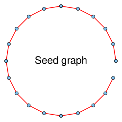
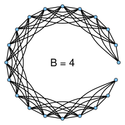
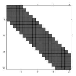
The right panel of Figure 1 shows a traditional -banded matrix. The term “banded” refers to the diagonal strip of nonzero elements that are within some distance (called the “bandwidth”) of the main diagonal. The middle panel of Figure 1 shows the graph with this adjacency matrix. Observing that this graph, denoted , is the -th power of the path graph shown in the left panel of Figure 1 suggests the following generalization of the term “banded.” We will use to denote the length of the shortest path between nodes and on .
Definition 1.
We say that a matrix is -banded with respect to a graph if , that is if .
Bickel & Lindner (2012) have a similar notion, for a metric , which they call -generalized banded operators.
Figure 2 shows the sparsity pattern of a -banded matrix with respect to a seed graph. The bandwidth can vary from , which corresponds to being a diagonal matrix, to being the diameter of , which corresponds to being a dense matrix when is a connected graph (when is not connected, the densest attainable is, up to permutation of the variables, a block-diagonal matrix with completely dense blocks).
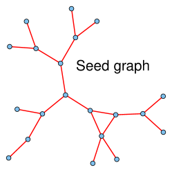
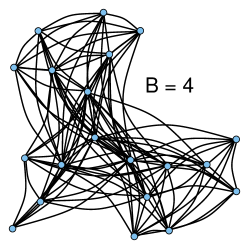

Despite the simple interpretation of taking powers of a seed graph, the resulting sparsity patterns can be quite complex and varied depending on the seed graph. There are many applications in which measured variables lie on a known graph that would be relevant to incorporate when estimating the covariance matrix :
-
•
Image data: Consider a pixeled image. The pixels lie on a two-dimensional lattice graph. Nearby pixels would be expected to be correlated.
-
•
fMRI data: One observes three-dimensional images of the brain over time. The voxels (three-dimensional pixels) lie on a three-dimensional lattice.
-
•
Social network data: A social media company wishes to estimate correlations between users’ purchasing behaviors (e.g., do they tend to buy the same items?). The social network of users is the known seed graph.
-
•
Gene expression data: Genes that encode proteins that are known to interact may potentially be more likely to be co-expressed than genes whose proteins do not interact. Biologists have constructed protein interaction networks (Das & Yu 2012), which may be taken as seed graphs, leveraging protein interaction data for better estimation of the covariance matrix of gene expression data.
In each example described above, the naive approach would be to vectorize the data and ignore the graph structure when estimating the covariance matrix. However, doing so when the truth is banded with respect to the known graph would be unnecessarily working in the patternless sparsity category when in fact a much simpler approach would work.
In some situations, a known seed graph is available, but the assumption of a single bandwidth applying globally is unrealistic. We can therefore extend the definition of bandedness with respect to a graph as follows:
Definition 2.
We say that a matrix is -banded with respect to a graph , if for all satisfying .
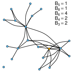
In words, this definition says that each variable has its own bandwidth, which defines a neighborhood size, and it cannot be correlated with any variables beyond this neighborhood. For example, on a social network, the bandwidth can be thought informally as having to do with the influence of a person. A very influential friend might be correlated with not just his friends but with his friends’ friends (this would correspond to ). By contrast, a “lone wolf” might be uncorrelated even with his own friends (). Figure 3 shows an example of a sparsity pattern emerging from the same seed graph as in Figure 2 but with variable bandwidths.


We propose two estimators in this paper that make use of a latent overlapping group lasso penalty (Jacob et al. 2009, Obozinski et al. 2011), which is used in situations in which one desires a sparsity pattern that is a union of a set of predefined groups. Both Definitions 1 and 2 can be described as such, so the difference between the two methods lies in the choice of groups. In Section 2, we introduce and study the graph-guided banding estimator, which produces estimates of the covariance matrix that are banded in the sense of Definition 1. The limited number of sparsity patterns attainable by this estimator makes it potentially undersirable in certain situations, and we therefore introduce and study (in Section 3) the graph-guided banding with local bandwidths estimator, which attains bandedness in the more flexible sense of Definition 2. Section 4 compares these methods empirically both in simulation and in naturally occurring data. Section 2.3 concludes with a discussion of related work, insights learned, and future directions.
To our knowledge, there is little work on using known graphs in high-dimensional covariance estimation. Cai & Yuan (2015) study minimax lower bounds and adaptive estimation of covariance matrices when variables lie on a -dimensional grid. Deng & Yuan (2009) consider inverse covariance estimation in the setting where variables lie in a metric space. Their approach uses a non-negative Garrotte semidefinite program formulation to perform inverse covariance estimation in which inverse covariance decays with increasing distance between variables. The method requires an initial estimate of the inverse covariance matrix (when , one takes ) and then shrinks so that variables farther apart have smaller partial covariances.
Notation: Given a matrix and a set of indices , we write to denote the matrix that agrees with on and is zero on , and we write for the cardinality of the set . The graph is the th power of , meaning the graph in which any nodes that are within of each other in are connected. The constraint means that the smallest eigenvalue of is at least . Given a square matrix , the matrix agrees with on off-diagonals but is zero on the diagonal. We write to mean that there exists a constant for which for sufficiently large.
2 Graph-guided banding with global bandwidth
Definition 1 introduces the simplest notion of bandedness with respect to a graph. In particular, a single bandwidth is postulated to apply globally across the entire graph. This means that the support of is given by one of the following groups of parameters:
| (1) |
where is the diameter of the seed graph . The group lasso (Yuan & Lin 2006) is a well-known extension of the lasso (Tibshirani 1996) that is useful for designing estimators in which groups of variables are simultaneously set to zero. Given a sample of independent random vectors , form the sample covariance matrix, . We define the graph-guided banding estimator with global bandwidth (GGB-global) as
| (2) |
where
is the latent overlapping group lasso penalty (Jacob et al. 2009) with group structure given by (1). Each matrix has the “graph-guided” sparsity pattern , so heuristically, this penalty favors that can be written as the sum of a small number of such sparse matrices. While the penalty is itself defined by an optimization problem, in practice we can solve (2) directly without needing to evaluate , as described in the next section.
The parameter will typically be taken to be ; however, in certain applications in which is very large and a reasonable upper bound on is available, it may be computationally expedient to choose a much smaller . The constraint only has an effect when . Of course, one must be cautious not to inadvertently choose since then the resulting estimates will always be sparser than the true covariance matrix. Thus, if one does not have a reliable upper bound for , one should simply take . The tuning parameter controls the sparsity level of (with large values of corresponding to greater sparsity). The are weights that control the relative strength of the individual norms in the penalty. In studying the theoretical properties of the estimator (Section 2.2), it becomes clear that is a good choice. The parameter is a user-specified lower bound on the eigenvalues of . While our algorithm is valid for any value of , the most common choice is , which ensures that is a positive semidefinite matrix. In certain applications, a positive definite matrix may be required, in which case the user may specify a small positive value for .
In the special case that is a path graph (and dropping the eigenvalue contraint), the GGB-global estimator reduces to the estimator introduced in Yan & Bien (2017). In the next section, we show that (2) can be efficiently computed.
2.1 Computation
The challenge of solving (2) lies in the combination of a nondifferentiable penalty and a positive semidefinite constraint. Without the penalty term, could be computed with a single thresholding of the eigenvalues; without the eigenvalue constraint, is nothing more than the proximal operator of evaluated at . The following lemma shows that we can solve (2) by alternate application of the proximal operator of and a thresholding of the eigenvalues. We present this result for general convex penalties since the same result will be used for the estimator introduced in Section 3.
Lemma 1.
Consider the problem
| (3) |
where is a closed, proper convex function, and let
denote the proximal operator of evaluated at a matrix . Algorithm 1 converges to .
Proof.
See Appendix A. ∎
-
•
Initialize .
-
•
Repeat until convergence:
-
1.
-
2.
where is the eigendecomposition.
-
1.
-
•
Return .
In Appendix A, we show that Algorithm 1 corresponds to blockwise coordinate ascent on the dual of (3). While the alternating direction method of multipliers (ADMM) would be an alternative approach to this problem, we prefer Algorithm 1 because, unlike ADMM, its use does not require choosing a suitable algorithm-specific parameter. Invoking the lemma, all that remains for solving (2) is to specify an algorithm for evaluating . The group structure (1) used in this estimator is special in that
Yan & Bien (2017) study the use of the latent overlapping group lasso with such hierarchically nested group structures and show that, for group structures of this form, the proximal operator can be evaluated essentially in closed form (which is not true more generally). Algorithm 3 of Yan & Bien (2017) shows that evaluating the proximal operator amounts to identifying a sequence of “breakpoints” and then applying groupwise soft-thresholding to the elements in for .
2.2 Theory
In this section, we study the statistical properties of the GGB estimator (2). For simplicity, we will focus on the special case in which (or, equivalently, we drop the eigenvalue constraint); however, in Section 2.2.3 we provide conditions under which our results apply to the case. We introduce two conditions under which we prove these results.
Assumption 1 (distribution of data).
We draw i.i.d. copies of , having mean and covariance . The random vector has bounded variances, , and sub-Gaussian marginals: for all . Both and are constants.
Assumption 2 (relation between and ).
We require that for some .
Assumptions 1 and 2 are sufficient for establishing that the sample covariance matrix concentrates around with high probability for large . These assumptions are made in Bien et al. (2015a), and similar assumptions appear throughout the literature.
2.2.1 Frobenius norm error
We begin by producing the rate of convergence of our estimator in Frobenius norm.
Theorem 1.
Proof.
See Appendix B. ∎
The term is the sparsity level of (with the initial representing the diagonal elements). Theorem 1 shows that when and moreover is , the GGB estimator is consistent in Frobenius norm. By contrast, consistency of the sample covariance matrix in this setting requires that be . Thus, when , GGB is expected to substantially outperform the sample covariance matrix. When , the theorem does not establish consistency of GGB. This fact is not, however, a shortcoming of the GGB method; rather, it is a reflection of the difficulty of the problem and the fact that the assumed sparsity level is in this case high relative to . Even when (i.e., is a diagonal matrix), we still must estimate free parameters on the basis of only observations. More generally, we know that the rate of convergence in Theorem 1 cannot, up to log factors, be improved by any other method. To see this, note that in the special case that is a path graph, Bien et al. (2015a) prove (in Theorem 7 of their paper) that the optimal rate is over the class of -banded matrices (assuming ). Since for a path graph, we see that the GGB estimator is within a log factor of the optimal rate in Frobenius norm.
If we are interested in estimating the correlation matrix instead of the covariance matrix, then we can apply our estimator to the sample correlation matrix . Because the diagonal entries of the correlation matrix do not need to be estimated, we can show (under one additional assumption) that the rate of convergence has in place of .
Assumption 3 (bounded non-zero variances).
Suppose that there exists a constant (i.e., not depending on or ) such that .
Theorem 2.
When has a small number of edges (e.g., with all but a small number of nodes having 0 degree), then we can have , in which case the above result establishes the consistency of the graph-guided estimator even when .
2.2.2 Bandwidth recovery
The remaining properties of this section can be established under a condition on the minimum signal strength (analogous to the “beta-min” conditions arising in the regression context).
Assumption 4 (minimum signal strength).
The nonzero elements of must be sufficiently large:
One can think of as on the order of and measuring the “noise level” of the data, in particular . Thus, this assumption ensures that the nonzeros stand out from the noise. Under this additional assumption, our estimator’s bandwidth, , matches the unknown bandwidth with high probability.
Theorem 3.
Proof.
See Appendix C. ∎
2.2.3 Positive semidefinite constraint
The results presented above are for . The next result provides an additional condition under which the previous results hold for the case (i.e., the situation in which the estimator is forced to be positive semidefinite).
Suppose all nonzero elements of are within a factor of of each other:
Assumption 5 (minimum eigenvalue).
The minimum eigenvalue of must be sufficiently large:
The quantity is the maximal degree of the true covariance graph (defined by the sparsity pattern of ).
2.3 Discussion & the small world phenomenon
The theorems above assume that , but the results in fact apply more generally so long as . While in general we may not know , there are some applications in which one may know enough about the mechanism of the graph-based dependence to provide an upper bound on . In such situations, choosing an that is much smaller than may lead to substantial computational improvements (both in terms of timing and memory).
Examining the Frobenius-norm bound above, we see that the structure of the seed graph plays an important role in the rates of convergence. While it is tempting to think of as controlling the sparsity level (and therefore the difficulty of the problem), it is important to observe that this quantity is in fact a function of both and the graph . For example, in the Frobenius-norm bound, the quantity is the number of pairs of variables that are within hops of each other in the graph . In conventional banded estimation, where is a path seed graph, the dependence on is linear: . More generally, when is a -dimensional lattice graph (when is small enough to avoid edge effects). However, intuition provided by lattice graphs does not extend well to more general graphs. For a particularly extreme example, when is a complete graph, then . Many large graphs in nature have small diameter (Watts & Strogatz 1998), which means that may be quite large even when is small. The idea of “six degrees of separation” (Travers & Milgram 1969) means that when using a social network as a seed graph, (in fact, recent work suggests six might even be an overestimate, Backstrom et al. 2011).
3 Graph-guided banding with local bandwidths
Definition 2 describes a different kind of graph-guided banding, in which each variable has an associated bandwidth , which can be thought of as a neighborhood size. Consider sets of the form
which is the set of variables within hops of in the seed graph . We can describe a sparsity pattern of the type in Definition 2 as
To see this, note that is equivalent to . We desire an estimator whose sparsity patterns are unions of the , so we use the latent overlapping group lasso penalty (Jacob et al. 2009), which is designed for such situations. We define the graph-guided banding estimator with local bandwidths (GGB-local) as
| (4) |
where
The only difference between this estimator and the GGB-global estimator of (2) is in the choice of groups. For a fixed , the groups are nested, . When is the diameter of the connected component that contains , then represents all variables that are connected to variable . For , we can have without one group contained completely in the other. The fact that this group structure is not simply hierarchically nested, as in the global bandwidth estimator, complicates both the computation and the theoretical analysis of the estimator.
3.1 Computation
By Lemma 1, we can solve (4) by Algorithm 1. The challenge of evaluating the GGB-local estimator lies therefore in efficiently evaluating the proximal operator . Viewing this problem as an optimization problem over the latent variables suggests a simple blockwise coordinate descent approach, which we adopt here.
3.2 Theory
In Theorem 1, we saw that the Frobenius-norm convergence depends on the number of nonzero off-diagonal elements, , a quantity that we observed in Section 2.3 could be quite large—as large as —even when is very small. In other words, for such “small-world” seed graphs , the assumption of graph-guided bandedness with a small global bandwidth does not necessarily correspond to being a sparse matrix. The notion of graph-guided bandedness with local bandwidths, as in Definition 2, provides finer control, allowing us to describe sparse even with “small-world” seed graphs . The purpose of the next theorem is to show that, under such a notion of sparsity, the GGB-local estimator can attain Frobenius-norm consistency when is sparse.
Theorem 5.
Proof.
See Appendix D. ∎
The two terms on the right-hand side of Theorem 5 represent estimation of the off-diagonal and diagonal elements of . If is sparse enough—in particular that , then estimating all of is as difficult as estimating its diagonal elements alone (i.e., just the variances). A simple example of this situation is when is -banded with respect to a graph and for at most variables . Another example is when all and the sum of degrees of all with is bounded by .
Theorem 5 suggests that consistency in Frobenius norm might not be achieved in the regime even in the sparsest situation of a diagonal matrix. As noted earlier, this is not a shortcoming of our method but rather a reflection of the difficulty of the task, which requires estimating independent parameters even in the sparsest situation of a diagonal matrix.
As noted previously, if instead we were interested in estimating the correlation matrix, we can attain a rate as in Theorem 5 but without the second term by applying our estimator to the sample correlation matrix.
Theorem 6.
Consistency follows even when as long as the right-hand side approaches 0.
4 Empirical study
4.1 Simulations
All simulations presented in this paper were performed using the simulator package (Bien 2016b, a) in R (R Core Team 2017). We investigate the advantages of exploiting a known graph structure (both in the global and local bandwidths settings), and we also study our two methods’ robustness to graph misspecification. We compare the two GGB methods to each other and to two other methods, which represent the “patternless sparsity” and traditional banding approaches.
Perhaps the simplest and most commonly used sparse covariance estimator is to simply soft-threshold each off-diagonal element of the sample covariance matrix:
This method (Rothman et al. 2009), along with its close relatives (Rothman 2012, Liu et al. 2013, Xue et al. 2012), do not make use of the graph and corresponds to (3) with being the norm and . Thus, comparisons to this method allow us to understand what is gained and what is lost by using the graph versus seeking “patternless sparsity.”
We also wish to compare our new estimators to a more traditional (i.e., non-graph-guided) banding approach. Graph-guided banding is not the only way one might incorporate the graph . A different approach would be to find an ordering of the nodes based on and then apply a traditional banding estimator with respect to this ordering. To this end, we seek an ordering of the variables that travels along as much as it can, making jumps to another part of as sparingly as possible. We express this as a traveling salesman problem (TSP), which we then solve using an off-the-shelf TSP solver (see Appendix F for details and for images of the learned paths). We then apply the convex banding method using this ordering (Bien et al. 2015a, b).
While each of these methods can be solved with a positive semidefinite constraint, we compare their performances without such a constraint. Doing so allows us to observe the fraction of the time each unconstrained estimator is positive semidefinite: Table 5 in Appendix G shows that the banding estimators are observed in the study to always be positive semidefinite, whereas this is not the case for the soft-thresholding estimator. It follows that the reported results for the banding methods in fact also pertain to these estimators with .
To generate a covariance matrix that is banded with respect to a graph , we take
where is chosen to ensure that the minimum eigenvalue of is at least (we take throughout).
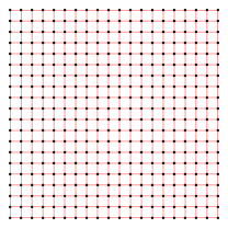
Initially, we compare the methods under four GGB structures: two-dimensional lattice with global bandwidth, two-dimensional lattice with local bandwidths, scale-free graph with global bandwidth, and scale-free graph with local bandwidths. In the first two scenarios, we take to be a two-dimensional square lattice having 20 variables per side (so ). The global bandwidth is taken to be , and the local bandwidths are generated according to
(see Figure 4).


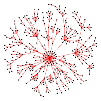

The resulting has roughly 10% of elements nonzero in the global case and about 1% in the local case. In the third and fourth scenarios, we take to be a scale free network (as generated by the function sample_pa in the R package igraph, Csardi & Nepusz 2006) with nodes. The same two choices of global and local bandwidths lead to having, respectively, about 75% and 10% nonzeros (see Figure 5). The marked difference in sparsity levels is a manifestation of the differing neighborhood structures between these two graph types.
4.1.1 Lattice versus scale-free graphs and global versus local bandwidths
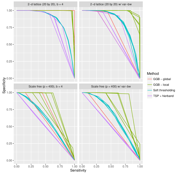
We generate samples of size under the four scenarios (and repeat 200 times). Tables 1 and 2 present Frobenius-norm error and operator-norm errors, and , respectively; table 3 presents the entropy error, . Each method has a single tuning parameter, and we report the performance of the method with the value of the tuning parameter chosen by 5-fold cross validation. In particular, we randomly partition the training data into 5 folds and, for an estimator , choose , where is the sample covariance matrix in which only the th fold is included and is the sample covariance matrix in which the th fold is omitted. In the 2-d lattice model, GGB-global does best when the true model has global bandwidth, as we would expect it to. Interestingly, GGB-local does best not just when the true model has local bandwidths but also in the scale-free model with a global bandwidth. This is a reminder of the important role that the seed graph’s structure plays in the statistical properties of the estimators. Finally, Figure 6 shows ROC curves for the four methods. The results are consistent with the results from the tables. In particular, GGB-global does best in the first scenario, and GGB-local does best in the other scenarios. Interestingly, TSP + hiernet does not appear to be an effective approach. Unlike the graph-guided approaches, TSP + hiernet does worse than soft-thresholding in nearly every scenario. For example, in Figure 6, we see that TSP + hiernet’s ability to identify nonzero elements of is no better than random guessing. This poor performance is to be expected in this scenario since such a network cannot be well captured by an ordering of the nodes. For the two-dimensional lattice graph scenarios, we find that such an approach is at least partially successful, which makes sense since the ordering captures some aspects of the underlying seed graph.
| GGB-global | GGB-local | Soft thresholding | TSP + hierband | |
|---|---|---|---|---|
| 2-d lattice (20 by 20), b = 4 | 7.605 (0.015) | 8.381 (0.031) | 11.634 (0.014) | 11.562 (0.031) |
| 2-d lattice (20 by 20) w/ var-bw | 4.244 (0.002) | 3.170 (0.008) | 4.347 (0.007) | 4.779 (0.003) |
| Scale free (p = 400), b = 4 | 6.740 (0.009) | 6.543 (0.015) | 7.655 (0.004) | 7.727 (0.009) |
| Scale free (p = 400) w/ var-bw | 3.273 (0.002) | 2.867 (0.007) | 3.552 (0.005) | 3.661 (0.002) |
| GGB-global | GGB-local | Soft thresholding | TSP + hierband | |
|---|---|---|---|---|
| 2-d lattice (20 by 20), b = 4 | 2.185 (0.007) | 2.428 (0.015) | 3.224 (0.010) | 3.149 (0.016) |
| 2-d lattice (20 by 20) w/ var-bw | 0.989 (0.003) | 0.756 (0.005) | 0.997 (0.004) | 1.024 (0.003) |
| Scale free (p = 400), b = 4 | 4.350 (0.010) | 4.110 (0.016) | 4.695 (0.004) | 4.709 (0.009) |
| Scale free (p = 400) w/ var-bw | 1.160 (0.001) | 1.008 (0.005) | 1.212 (0.002) | 1.238 (0.001) |
| GGB-global | GGB-local | Soft thresholding | TSP + hierband | |
|---|---|---|---|---|
| 2-d lattice (20 by 20), b = 4 | 7719 ( 24) | 7819 ( 69) | 10234 ( 34) | 11870 ( 73) |
| 2-d lattice (20 by 20) w/ var-bw | 25823 ( 55) | 18088 (119) | 25358 ( 89) | 27188 ( 62) |
| Scale free (p = 400), b = 4 | 72606 (146) | 68087 (191) | 68654 ( 62) | 68518 (119) |
| Scale free (p = 400) w/ var-bw | 52047 ( 70) | 44188 (186) | 53332 ( 86) | 54304 ( 76) |
4.1.2 Effect of graph misspecification
The previous simulation studies establish the rather obvious fact that when one knows the true graph with respect to which is banded, one can better estimate with an estimator that uses . In practice, however, one might typically use a graph that is (hopefully) close to but not exactly identical. This section seeks to understand the effect of graph misspecification on the effectiveness of graph-guided banding. We simulate data as above but imagine that we only have access to a corrupted version of the underlying graph .
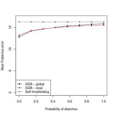
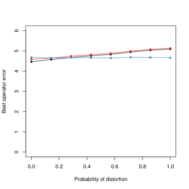
Let control the degree of corruption to . Of course there are many ways to corrupt a graph, but we choose a scheme that will preserve the properties of the graph and the sparsity level of the covariance matrix (so as not to confound graph distortion with other factors such as sparsity level, number of triangles, etc.). In particular, we take to be an Erdos-Renyi graph with vertices and edges (this is chosen to match the number of edges in the previous examples). We take to have global graph-guided bandwidth with respect to this graph . For each edge in , with probability we remove it and then connect two currently unconnected nodes chosen at random. We choose to be an Erdos-Renyi graph so that the distorted graph is itself Erdos-Renyi with the same number of edges. By keeping all graph properties fixed, we can be confident that as we vary , any differences in performance of the methods will be attributable to and having different edges.
Figure 7 shows the performance of the three methods as the probability of reassigning an edge is varied from 0 (no distortion of ) to 1 (all edges are distorted). As expected, we see both GGB methods deteriorating as the distortion level of the seed graph is increased. When (i.e., ) GGB-global is best (which makes sense since has a global bandwidth). When approximately of the edges are distorted, the best obtainable operator-norm error by the GGB methods becomes worse than that of soft-thresholding. Soft-thresholding is, of course, unaffected by graph distortion since it does not use at all. Surprisingly, in Frobenius-norm error the two GGB methods remain better than soft-thresholding even at very high levels of distortion. A deeper examination of this simulation reveals that the GGB methods are more biased but less variable than the soft-thresholding estimates, leading to a smaller Frobenius-norm error. We do expect this behavior to be problem-specific and in general would expect GGB methods with highly distorted graphs to perform worse than soft-thresholding.
4.2 Application to images of handwritten digits
In this section, we apply our estimators to a dataset of ()-pixel images of handwritten digits (Le Cun et al. 1990, Hastie et al. 2009)111available at http://statweb.stanford.edu/~tibs/ElemStatLearn/datasets/zip.digits/. There are between (roughly) 700 and 1500 images per digit type. For each digit type, we take a random images to form the “training set” sample covariance matrix and use the remaining data to form the “test set” sample covariance matrix (our results are based on 20 replications of this process). A natural seed graph in this situation is the two-dimensional lattice graph formed by connecting adjacent pixels. We compare our two GGB estimators to the soft-thresholding estimator. We fit each covariance estimator to the training data and compute its best attainable (over choice of tuning parameter) distance in Frobenius norm to ,
Table 4 reports this quantity, averaged over the 20 random train-test splits of the dataset, for each digit. GGB-local has a lower test error than soft-thresholding in all 20 replicates for the digits 2-9; GGB-global has a lower test error than soft-thresholding in all 20 replicates for all digits other than 0, 1, and 6. In fact, there is no digit for which soft-thresholding wins in a majority of replicates. This indicates that exploiting the neighborhood structure inherent to image data is useful for covariance estimates in this context.
| GGB-global | GGB-local | Soft thresholding | |
|---|---|---|---|
| Digit 0 | 10.8 (0.1) | 10.8 (0.1) | 11.0 (0.1) |
| Digit 1 | 2.6 (0.1) | 2.6 (0.1) | 2.6 (0.1) |
| Digit 2 | 10.9 (0.2) | 10.9 (0.2) | 11.3 (0.1) |
| Digit 3 | 8.9 (0.1) | 8.9 (0.1) | 9.3 (0.1) |
| Digit 4 | 9.4 (0.1) | 9.5 (0.1) | 9.9 (0.1) |
| Digit 5 | 10.7 (0.2) | 10.8 (0.2) | 11.2 (0.2) |
| Digit 6 | 9.2 (0.2) | 9.1 (0.2) | 9.2 (0.2) |
| Digit 7 | 7.3 (0.1) | 7.4 (0.1) | 7.5 (0.1) |
| Digit 8 | 9.3 (0.1) | 9.4 (0.1) | 9.8 (0.1) |
| Digit 9 | 7.8 (0.2) | 7.9 (0.2) | 8.0 (0.2) |
5 Discussion
This paper generalizes the notion of banded covariance estimation to situations in which there is a known underlying graph structure to the variables being measured. The traditional notion of a banded matrix corresponds to the special case where this graph is a path encoding the ordering of the variables. We propose two new “graph-guided” estimators, based on convex optimization problems: GGB-global enforces a single bandwidth across all variables while GGB-local allows each variable to have its own bandwidth. There are many interesting avenues of future research. In this paper, we assume the seed graph is given, and the challenge is in determining the bandwidth(s). One could imagine situations in which the seed graph itself is unavailable (but in which we do believe that such a graph exists). In such a setting, can one identify the smallest seed graph for which the covariance matrix’s sparsity pattern is banded with respect to ? This generalizes the problem of discovering an ordering for which one can apply a traditional known-ordering estimator considered by Wagaman & Levina (2009), Zhu & Liu (2009). A simple heuristic strategy might involve forming a minimum spanning tree based on the complete graph with edge weights given by the sample covariance matrix. The graph-guided banding estimators would then have sparsity patterns with this minimum spanning tree seed graph serving as backbone. Another future avenue of research is in applying the graph-guided structure to the inverse covariance matrix. Finally, we have seen (e.g., in Theorem 1 and in the empirical study) that the properties of the seed graph influence the success of the GGB estimators. More generally understanding how the graph properties of affect the difficulty of the estimation problem itself would be a particularly interesting direction of future study.
Appendix A Proof of Lemma 1 of main paper
Lemma 2.
Consider the problem
where is a closed, proper convex function, and let
denote the proximal operator of evaluated at a matrix . Algorithm 1 converges to .
Proof.
Problem (3) is equivalent to
which has Lagrangian
The dual function is given by minimizing over and :
where is the convex conjugate of . Also,
The dual optimal is given by solving
which is a convex problem. Furthermore, by Tseng (2001), it can be solved by alternately optimizing over (holding fixed) and over (holding fixed). The solution to the optimization over is the proximal operator of evaluated at . The Moreau decomposition (see, e.g., Parikh & Boyd 2014) for the closed, proper convex function gives us
Optimizing over while holding fixed requires solving
which in terms of the eigenvalue decomposition of becomes
or where
which is solved by
∎
Appendix B Proof of Theorem 1 of main paper (Frobenius error)
Proof.
Since and , the estimator is more simply
| (5) |
where
In what follows, whenever we write a sum with subscript , it is understood to run along ; this also holds for the notation, which is short for .
We begin by observing that (5) is a strongly convex problem in , and thus there is a unique minimizer , although the minimizing set of ’s may not be unique. Also, since does not appear in the penalty, we see that . Thus, we can write (5) as
| (6) |
We can write (6) in terms of the ’s:
| (7) |
Note that we have replaced by (for notational convenience) since does not include diagonal elements. The lemma below provides necessary and sufficient conditions for to be a solution to (7).
Lemma 3.
Proof.
Problem (7) is equivalent to a non-overlapping group lasso problem, and this lemma provides the KKT conditions of this problem, which are well-known. ∎
Corollary 1.
Let be a solution to (7). Then,
Suppose . If we can construct a solution to (7) that has
then, by Corollary 1, we know that for all or
In fact, the corollary implies that this holds for all solutions, not just for our constructed .
Consider the restricted problem
and write . This restricted problem is of an identical form to (7) but with replaced by . Thus, Lemma 3 applies if we replace with : For each ,
and otherwise.
Now, for , let . We show that is a solution to (7). Clearly, , so by Lemma 3 it simply remains to show that
For :
Now, on the event
| (8) |
we have
using that . This establishes, by Lemma 3, that is a solution to (7) and, by Corollary 1 that for all solutions to (7). Given the support constraints of each , it follows that the overall has bandwidth no larger than .
Proposition 1.
If , , and , then on .
Having established the above proposition about the bandwidth, it is straightforward to prove a result about the estimation error. On ,
and . Thus,
| (9) |
Proposition 2.
If , , and , then
on .
Appendix C Proof of Theorem 3 of main paper (bandwidth recovery)
We prove a result that is a bit more general than Theorem 3 of the main paper.
Theorem 1.
Under the minimum signal condition
and the conditions of Theorem 1 of the main paper, with probability at least .
Proof.
We already know that , so it suffices to show that
which follows since
The result then follows from (10). ∎
Corollary 2.
Under the minimum signal condition
and the conditions of Theorem 1 of the main paper, with probability at least .
Proof.
Appendix D Proof of Theorem 5 (Frobenius error of local bandwidths estimator)
Proof.
Let be the minimizer of Equation (4) of the main paper. By definition,
Since
we have
| (11) |
By Lemma 3 of Obozinski et al. (2011), the dual norm is , and so
| (12) |
Define the index sets and .
Observe that with
It follows that
as long as , that is on the event , as defined in (8). Thus, combining this with (11),
holds on . Using the triangle inequality ( is a norm),
By definition of ,
| (13) |
for any choice of such that and .
Consider taking , for all and , unless
-
(i)
, in which case we take
-
(ii)
, in which case we take
-
(iii)
, in which case we take
We verify that this choice of satisfies the necessary constraints. Clearly, for . If , then , which excludes cases (i) and (ii), the only two cases in which (and ) could be nonzero. Thus, .
We next verify that . In case (i),
In case (ii),
In case (iii),
Now, we have that , which implies that . Thus,
Appendix E Proofs about GGB on sample correlation matrix
We begin by establishing a concentration inequality for the correlation matrix that will be used in the proofs of both of these theorems. This result is similar to Lemma A.2 of Liu et al. (2017) except that we assume sub-Gaussian rather than Gaussian data. It is also similar to Lemma D.5 of Sun et al. (2017) except that we assume that has been centered by the sample mean.
Lemma 4.
Proof.
The following proof is based on the proof of Lemma A.2 of Liu et al. (2017). Certain details have been fleshed out and some modifications have been made to accommodate the differing assumptions.
Let . Observing that , it follows that
| (14) |
Now,
By (14) and the triangle inequality,
so
Now,
Since , and thus we have established that
By Lemma A.1 of Bien et al. (2015c) (with a typo corrected), there exist constants such that
for any . This constraint on implies that and so
Taking ,
Observing that , we have that
We take for . By Assumption 3, and are treated as constants. If then and
Thus, we just need that , which can be ensured by choosing
∎
We define the event
| (15) |
Lemma 4 establishes that there exist constants and for which choosing ensures that .
E.1 Proof of Theorem 2 (Frobenius error of global GGB on correlation matrix)
Let be the minimizer of Equation (2) of the main paper where is replaced by .
E.2 Proof of Theorem 6 (Frobenius error of local GGB on correlation matrix)
Let be the minimizer of Equation (4) of the main paper where is replaced by .
Appendix F Traveling salesman problem
Let be a matrix of costs, with being the cost of traveling from node to node . The traveling salesman problem (TSP) seeks a loop through all the nodes such that is minimal.
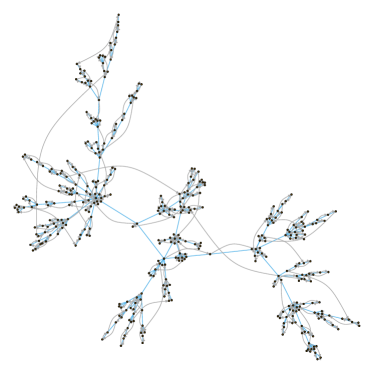
In our context, we have a graph and wish to find an ordering of the nodes that is strongly informed by . In particular, we would like this path to travel along edges of as much as possible and when this is not possible and the path must “fly” between two nodes that are not connected by a node, that it take the shortest flight possible. We therefore take
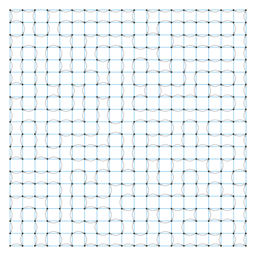
We use the R package TSP (Hahsler & Hornik 2017), which provides an interface to the Concorde solver (Applegate et al. 2017), and Figure 8 shows the resulting paths.
Appendix G An empirical study of positive semidefiniteness
For each of the models considered in Section 4.1.1 of the main paper, we record the proportion of the time each method is positive semidefinite. In particular, this average is over both the 200 simulation replicates and the values of the tuning parameter of each method. Table 5 shows that throughout this study the banding methods (GGB and hierband) are always observed to give positive semidefinite estimates. This is not the case for the soft-thresholding estimator.
| GGB - global | GGB - local | Soft thresholding | TSP + hierband | |
| 2-d lattice (20 by 20), b = 4 | 1.000 (0.000) | 1.000 (0.000) | 0.349 (0.008) | 1.000 (0.000) |
| 2-d lattice (20 by 20) w/ var-bw | 1.000 (0.000) | 1.000 (0.000) | 0.625 (0.008) | 1.000 (0.000) |
| Scale free (p = 400), b = 4 | 1.000 (0.000) | 1.000 (0.000) | 0.998 (0.001) | 1.000 (0.000) |
| Scale free (p = 400) w/ var-bw | 1.000 (0.000) | 1.000 (0.000) | 1.000 (0.000) | 1.000 (0.000) |
Appendix H A higher dimensional example
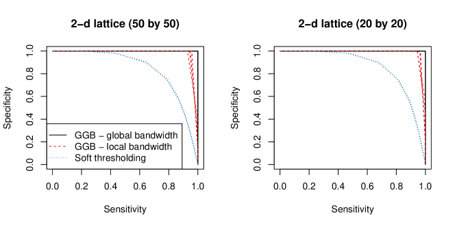
In Section 4.1.1, we study four models in which and . The covariance matrix has parameters. Thus, the number of parameters to be estimated greatly exceeds the number of samples. Nonetheless, we can ask what happens if is even larger than this. We revisit the example of the 2-d lattice, increasing the side length from 20 to 50 so that . In this case the covariance matrix has parameters. We focus in particular on the GGB methods and soft thresholding. Figure 9 provides a side-by-side comparison of the ROC curves (five replicates are shown per method) when one increases from to . The curves in the two plots are different although this is difficult to discern by eye. This suggests that we are effectively in the same regime in these two simulated scenarios.
References
- (1)
-
Applegate et al. (2017)
Applegate, D., Bixby, R., Chvatal, V. & Cook, W. (2017), Concorde TSP Solver.
http://www.math.uwaterloo.ca/tsp/concorde/ - Backstrom et al. (2011) Backstrom, L., Boldi, P., Rosa, M., Ugander, J. & Vigna, S. (2011), ‘Four degrees of separation. doi: arxiv1111. 4570v1’.
- Banerjee et al. (2008) Banerjee, O., El Ghaoui, L. E. & d’Aspremont, A. (2008), ‘Model selection through sparse maximum likelihood estimation for multivariate gaussian or binary data’, Journal of Machine Learning Research 9, 485–516.
- Bickel & Levina (2008a) Bickel, P. J. & Levina, E. (2008a), ‘Regularized estimation of large covariance matrices’, Annals of Statistics pp. 199–227.
- Bickel & Levina (2008b) Bickel, P. & Levina, E. (2008b), ‘Covariance regularization by thresholding’, Annals of Statistics 36, 2577–2604.
- Bickel & Lindner (2012) Bickel, P. & Lindner, M. (2012), ‘Approximating the inverse of banded matrices by banded matrices with applications to probability and statistics’, Theory of Probability & Its Applications 56(1), 1–20.
-
Bien (2016a)
Bien, J. (2016a), simulator: An
Engine for Running Simulations.
R package version 0.2.0.
https://CRAN.R-project.org/package=simulator - Bien (2016b) Bien, J. (2016b), ‘The simulator: An engine to streamline simulations’, arXiv preprint arXiv:1607.00021 .
- Bien et al. (2015a) Bien, J., Bunea, F. & Xiao, L. (2015a), ‘Convex banding of the covariance matrix’, Journal of the American Statistical Association DOI: 10.1080/01621459.2015.1058265 .
-
Bien et al. (2015b)
Bien, J., Bunea, F. & Xiao, L. (2015b), hierband: Convex Banding of the Covariance
Matrix.
R package version 1.0.
https://CRAN.R-project.org/package=hierband - Bien et al. (2015c) Bien, J., Bunea, F. & Xiao, L. (2015c), ‘Supplementary materials to “convex banding of the covariance matrix”’, Journal of the American Statistical Association .
- Bien & Tibshirani (2011) Bien, J. & Tibshirani, R. (2011), ‘Sparse estimation of a covariance matrix’, Biometrika 98(4), 807–820.
- Cai et al. (2011) Cai, T., Liu, W. & Luo, X. (2011), ‘A constrained l1 minimization approach to sparse precision matrix estimation’, Journal of the American Statistical Association 106(494), 594–607.
- Cai & Yuan (2012) Cai, T. T. & Yuan, M. (2012), ‘Adaptive covariance matrix estimation through block thresholding’, The Annals of Statistics 40(4), 2014–2042.
- Cai & Yuan (2015) Cai, T. T. & Yuan, M. (2015), ‘Minimax and adaptive estimation of covariance operator for random variables observed on a lattice graph’, Accepted to Journal of the American Statistical Association .
- Cai et al. (2010) Cai, T. T., Zhang, C.-H. & Zhou, H. H. (2010), ‘Optimal rates of convergence for covariance matrix estimation’, The Annals of Statistics 38(4), 2118–2144.
- Chandrasekaran et al. (2010) Chandrasekaran, V., Parrilo, P. A. & Willsky, A. S. (2010), Latent variable graphical model selection via convex optimization, in ‘Communication, Control, and Computing (Allerton), 2010 48th Annual Allerton Conference on’, IEEE, pp. 1610–1613.
-
Csardi & Nepusz (2006)
Csardi, G. & Nepusz, T. (2006),
‘The igraph software package for complex network research’, InterJournal Complex Systems, 1695.
http://igraph.org - Das & Yu (2012) Das, J. & Yu, H. (2012), ‘Hint: High-quality protein interactomes and their applications in understanding human disease’, BMC systems biology 6(1), 92.
- Dempster (1972) Dempster, A. P. (1972), ‘Covariance selection’, Biometrics 28(1), 157–175.
- Deng & Yuan (2009) Deng, X. & Yuan, M. (2009), ‘Large gaussian covariance matrix estimation with markov structures’, Journal of Computational and Graphical Statistics 18(3).
- Donoho et al. (2013) Donoho, D. L., Gavish, M. & Johnstone, I. M. (2013), ‘Optimal shrinkage of eigenvalues in the spiked covariance model’, arXiv preprint arXiv:1311.0851 .
- Fan et al. (2008) Fan, J., Fan, Y. & Lv, J. (2008), ‘High dimensional covariance matrix estimation using a factor model’, Journal of Econometrics 147(1), 186–197.
- Fan et al. (2013) Fan, J., Liao, Y. & Mincheva, M. (2013), ‘Large covariance estimation by thresholding principal orthogonal complements’, Journal of the Royal Statistical Society: Series B (Statistical Methodology) 75(4), 603–680.
- Friedman et al. (2008) Friedman, J., Hastie, T. & Tibshirani, R. (2008), ‘Sparse inverse covariance estimation with the graphical lasso’, Biostatistics 9, 432–441.
-
Hahsler & Hornik (2017)
Hahsler, M. & Hornik, K. (2017),
TSP: Traveling Salesperson Problem (TSP).
R package version 1.1-5.
https://CRAN.R-project.org/package=TSP - Hastie et al. (2009) Hastie, T., Tibshirani, R. & Friedman, J. (2009), The Elements of Statistical Learning; Data Mining, Inference and Prediction, Second Edition, Springer Verlag, New York.
- Huang et al. (2006) Huang, J., Liu, N., Pourahmadi, M. & Liu, L. (2006), ‘Covariance matrix selection and estimation via penalised normal likelihood’, Biometrika 93(1), 85.
- Jacob et al. (2009) Jacob, L., Obozinski, G. & Vert, J.-P. (2009), Group lasso with overlap and graph lasso, in ‘Proceedings of the 26th annual international conference on machine learning’, ACM, pp. 433–440.
- Johnstone (2001) Johnstone, I. M. (2001), ‘On the distribution of the largest eigenvalue in principal components analysis’, Annals of statistics pp. 295–327.
- Khare et al. (2014) Khare, K., Oh, S.-Y. & Rajaratnam, B. (2014), ‘A convex pseudolikelihood framework for high dimensional partial correlation estimation with convergence guarantees’, Journal of the Royal Statistical Society: Series B (Statistical Methodology) .
- Lam & Fan (2009) Lam, C. & Fan, J. (2009), ‘Sparsistency and rates of convergence in large covariance matrix estimation’, Annals of Statistics 37(6B), 4254–4278.
- Le Cun et al. (1990) Le Cun, B. B., Denker, J. S., Henderson, D., Howard, R. E., Hubbard, W. & Jackel, L. D. (1990), Handwritten digit recognition with a back-propagation network, in ‘Advances in neural information processing systems’, Citeseer.
- Ledoit & Wolf (2004) Ledoit, O. & Wolf, M. (2004), ‘A well-conditioned estimator for large-dimensional covariance matrices’, Journal of multivariate analysis 88(2), 365–411.
- Levina et al. (2008) Levina, E., Rothman, A. & Zhu, J. (2008), ‘Sparse estimation of large covariance matrices via a nested lasso penalty’, The Annals of Applied Statistics pp. 245–263.
- Liu et al. (2013) Liu, H., Wang, L. & Zhao, T. (2013), ‘Sparse covariance matrix estimation with eigenvalue constraints’, Journal of Computational and Graphical Statistics .
- Liu et al. (2017) Liu, H., Wang, L. et al. (2017), ‘Tiger: A tuning-insensitive approach for optimally estimating gaussian graphical models’, Electronic Journal of Statistics 11(1), 241–294.
- Luo (2011) Luo, X. (2011), ‘Recovering model structures from large low rank and sparse covariance matrix estimation’, arXiv preprint arXiv:1111.1133 .
- Meinshausen & Bühlmann (2006) Meinshausen, N. & Bühlmann, P. (2006), ‘High dimensional graphs and variable selection with the lasso’, Annals of Statistics 34, 1436–1462.
- Obozinski et al. (2011) Obozinski, G., Jacob, L. & Vert, J. (2011), ‘Group lasso with overlaps: The latent group lasso approach’, arXiv preprint arXiv:1110.0413 .
- Parikh & Boyd (2014) Parikh, N. & Boyd, S. P. (2014), ‘Proximal algorithms.’, Foundations and Trends in optimization 1(3), 127–239.
- Peng et al. (2009) Peng, J., Wang, P., Zhou, N. & Zhu, J. (2009), ‘Partial correlation estimation by joint sparse regression models’, Journal of the American Statistical Association 104(486).
-
R Core Team (2017)
R Core Team (2017), R: A Language and
Environment for Statistical Computing, R Foundation for Statistical
Computing, Vienna, Austria.
https://www.R-project.org/ - Rothman (2012) Rothman, A. (2012), ‘Positive definite estimators of large covariance matrices’, Biometrika 99(3), 733–740.
- Rothman et al. (2009) Rothman, A. J., Levina, E. & Zhu, J. (2009), ‘Generalized thresholding of large covariance matrices’, Journal of the American Statistical Association 104(485), 177–186.
- Rothman et al. (2008) Rothman, A., Levina, E. & Zhu, J. (2008), ‘Sparse permutation invariant covariance estimation’, Electronic Journal of Statistics 2, 494–515.
- Rothman et al. (2010) Rothman, A., Levina, E. & Zhu, J. (2010), ‘A new approach to Cholesky-based covariance regularization in high dimensions’, Biometrika 97(3), 539.
- Sun et al. (2017) Sun, Q., Tan, K. M., Liu, H. & Zhang, T. (2017), ‘Graphical nonconvex optimization for optimal estimation in gaussian graphical models’, arXiv preprint arXiv:1706.01158 .
- Tibshirani (1996) Tibshirani, R. (1996), ‘Regression shrinkage and selection via the lasso’, J. Royal. Stat. Soc. B. 58, 267–288.
- Travers & Milgram (1969) Travers, J. & Milgram, S. (1969), ‘An experimental study of the small world problem’, Sociometry pp. 425–443.
- Tseng (2001) Tseng, P. (2001), ‘Convergence of a block coordinate descent method for nondifferentiable minimization’, Journal of optimization theory and applications 109(3), 475–494.
- Wagaman & Levina (2009) Wagaman, A. & Levina, E. (2009), ‘Discovering sparse covariance structures with the isomap’, Journal of Computational and Graphical Statistics 18(3), 551–572.
- Watts & Strogatz (1998) Watts, D. J. & Strogatz, S. H. (1998), ‘Collective dynamics of ‘small-world’ networks’, Nature 393(6684), 440–442.
-
Wickham (2009)
Wickham, H. (2009), ggplot2: elegant
graphics for data analysis, Springer New York.
http://had.co.nz/ggplot2/book - Won et al. (2013) Won, J.-H., Lim, J., Kim, S.-J. & Rajaratnam, B. (2013), ‘Condition-number-regularized covariance estimation’, Journal of the Royal Statistical Society: Series B (Statistical Methodology) 75(3), 427–450.
- Wu & Pourahmadi (2003) Wu, W. B. & Pourahmadi, M. (2003), ‘Nonparametric estimation of large covariance matrices of longitudinal data’, Biometrika 90(4), 831–844.
- Wu & Pourahmadi (2009) Wu, W. B. & Pourahmadi, M. (2009), ‘Banding sample autocovariance matrices of stationary processes’, Statistica Sinica 19(4), 1755.
- Xue et al. (2012) Xue, L., Ma, S. & Zou, H. (2012), ‘Positive-definite l1-penalized estimation of large covariance matrices’, Journal of the American Statistical Association 107(500), 1480–1491.
- Yan & Bien (2017) Yan, X. & Bien, J. (2017), ‘Hierarchical sparse modeling: A choice of two group lasso formulations’, Statistical Science 32(4), 531–560.
- Yu & Bien (2017) Yu, G. & Bien, J. (2017), ‘Learning local dependence in ordered data’, Journal of Machine Learning Research 18(42), 1–60.
- Yuan (2010) Yuan, M. (2010), ‘High dimensional inverse covariance matrix estimation via linear programming’, The Journal of Machine Learning Research 11, 2261–2286.
- Yuan & Lin (2006) Yuan, M. & Lin, Y. (2006), ‘Model selection and estimation in regression with grouped variables’, Journal of the Royal Statistical Society, Series B 68, 49–67.
- Yuan & Lin (2007) Yuan, M. & Lin, Y. (2007), ‘Model selection and estimation in the Gaussian graphical model’, Biometrika 94(1), 19–35.
- Zhu & Liu (2009) Zhu, Z. & Liu, Y. (2009), ‘Estimating spatial covariance using penalised likelihood with weighted l1 penalty’, Journal of Nonparametric Statistics 21(7), 925–942.