The Importance of Worker Reputation Information
in Microtask-Based Crowd Work Systems

Abstract

This paper presents the first systematic investigation of the potential performance gains for crowd work systems, deriving from available information at the requester about individual worker reputation. In particular, we first formalize the optimal task assignment problem when workers’ reputation estimates are available, as the maximization of a monotone (submodular) function subject to Matroid constraints. Then, being the optimal problem NP-hard, we propose a simple but efficient greedy heuristic task allocation algorithm. We also propose a simple “maximum a-posteriori” decision rule and a decision algorithm based on message passing. Finally, we test and compare different solutions, showing that system performance can greatly benefit from information about workers’ reputation. Our main findings are that: i) even largely inaccurate estimates of workers’ reputation can be effectively exploited in the task assignment to greatly improve system performance; ii) the performance of the maximum a-posteriori decision rule quickly degrades as worker reputation estimates become inaccurate; iii) when workers’ reputation estimates are significantly inaccurate, the best performance can be obtained by combining our proposed task assignment algorithm with the message-passing decision algorithm.

I Introduction

Crowd work is a term often adopted to identify networked systems that can be used for the solution of a wide range of complex problems by integrating a large number of human and/or computer efforts [1]. Alternative terms, each one carrying its own specific nuance, to identify similar types of systems are: collective intelligence, human computation, master-worker computing, volunteer computing, serious games, voting problems, peer production, citizen science (and others). An entire host of general-purpose or specialized online platforms, such as information-sharing platforms for recommendations (e.g., Tripadvisor, Amazon), co-creation systems (e.g., Wikipedia, Gnu project), social-purpose communities for urban mobility (e.g., Waze), microtask-based crowd work systems, etc., can be defined under these terms.

In this paper, we specialize to microtask-based crowd work systems. The key characteristic of these systems is that a requester structures his problem in a set of tasks, and then assigns tasks to workers that provide answers, which are then used to determine the correct task solution through a decision rule. A well-known example of such systems is Amazon Mechanical Turk (MTurk), which allows the employment of large numbers of low-wage workers for tasks requiring human intelligence (HIT – Human Intelligence Tasks). Examples of HIT are image classification, annotation, rating and recommendation, speech labeling, proofreading, etc. In the Amazon Mechanical Turk, the workload submitted by the requester is partitioned into several microtasks, with a simple and strictly specified structure, which are then assigned to (human) workers. Since task execution is typically tedious, and the economic reward for workers is pretty small, workers are not 100% reliable, in the sense that they may provide incorrect answers. Hence, in most practical cases, the same task is assigned in parallel (replicated) to several workers, and then a majority decision rule is applied to their answers. A natural trade-off between reliability of the decision and cost arises; indeed, by increasing the replication factor of every task, we generally increase the reliability degree of the final decision about the task solution, but we necessarily incur higher costs (or, for a given fixed cost, we obtain a lower task throughput). Although the pool of workers in crowd work systems is normally large, it can be abstracted as a finite set of shared resources, so that the allocation of tasks to workers (or, equivalently, of workers to tasks) is of key relevance to the system performance. Some believe that microtask-based crowd work systems will provide a significant new type of work organization paradigm, and will employ ever increasing [2] numbers of workers in the future, provided that the main challenges in this new type of organizations are correctly solved. In [3] the authors identify a dozen such challenges, including i) workflow definition and hierarchy, ii) task assignment, iii) real-time response, iv) quality control and reputation. All these aspects can represent an interesting research subject and some of them have already stimulated a large bulk of literature, as it will be detailed in the next subsection. However, this paper deals mainly with task assignment and with the quantitative assessment of the gain (in terms of increased decision reliability for a given cost) that a coarse knowledge of worker quality can offer. Indirectly, thus, we deal also with worker reputation, although we do not study mechanisms through which reputation is built upon time. Indeed, we consider a one-shot approach in which the requester has to assign a bunch of tasks to a pool of workers that are statically divided into classes according to their probabilities of answering correctly. We highlight that the way this division into classes is built is out of the scope of this paper, although we will analyze the effect of errors in this classification on the decision reliability.

I-A Previous work

In current online platforms, task assignment is either implemented through a simple first-come/first-served rule, or according to more sophisticated approaches. In MTurk, the requester can specify the number of workers to be assigned to each task. MTurk also gives requesters the possibility of dismissing low-quality answers, so that each experienced worker is characterized by an approval rating. As a consequence, the requester is also allowed to prescribe a given qualification level for workers to be able to access her tasks. An analysis of the correlation between MTurk approval rating and worker quality is performed in [4]. In the scientific community, the task assignment in crowdsourcing systems has recently been formalized [5, 6, 7, 8] as a resource allocation problem, under the assumption that both tasks and workers are indistinguishable. On the worker side, this assumption is motivated by the fact that the implementation of reputation-tracing mechanisms for workers may be challenging, because the workers’ pool is typically large and highly volatile. A step ahead has been recently made in [9], which proposes an adaptive online algorithm to assign an appropriate number of workers to every task, so as to meet a prefixed constraint on the problem solution reliability. Like in this paper, in [9] workers are partitioned in different classes, with workers within each class meeting a specified reliability index. However, unlike this paper, the allocation algorithm of [9] is adaptive, i.e., it is based on previous answers on the same set of microtasks: an assumption that, although certainly interesting, implies a time-consuming overall process of task accomplishment. The same adaptive approach is followed in [10], where a bandit-based algorithm is adopted to allocate heterogeneous tasks to workers with task-dependent skills. Given a pool of $n$ questions, [11] investigates how $k$ questions therefrom should be assigned to a worker.

Most real-world crowdsourcing systems typically implement a majority-based decision rule to obtain task solutions. In the last few years, in the scientific literature, smarter decision rules have been proposed to improve the performance of crowdsourcing systems, for the case where no a-priori information about workers’ reputation is available (i.e. workers are a-priori indistinguishable) while tasks are homogeneously difficult [5, 6, 7, 8, 12, 13]. Essentially the same decision strategy was proposed in [5, 6] and [8] for the case in which tasks require binary answers, and then recently extended in [7] and, independently, in [14], to the case in which tasks require generic multiple-choice answers. In [6, 7] it is shown that the improved decision rule can be efficiently implemented employing a message-passing technique. In [12], an integrated estimation-allocation approach has been pursued with Bayesian inference and entropy reduction as utility function. Different methodologies based on the Expectation-Maximization algorithm have been proposed in [15, 13]. All these algorithms exploit existing redundancy and correlation in the pattern of answers returned from workers to infer an a-posteriori reliability estimate for every worker. The derived estimates are then used to properly weigh workers’ answers. When there is a-priori information about workers’ reliability, to the best of our knowledge, the only decision rule proposed in the literature is weighted average, like, e.g., in [10].

There is a wide literature about workers’ motivation and reputation. Regarding motivation, many studies report experiments conducted on MTurk as a paradigm of microtask-based crowd work platform. Classical studies of offline work reveal that workers try to understand which activities are better rewarded and tend to prefer those, virtually excluding others [16]. However, in the context of crowdsourcing systems, mixed results have been shown about the effect of economic incentives on the quality of workers’ outputs [17, 18, 19, 20, 21, 22]. These studies highlight the importance of intrinsically non-economical motivations such as the feeling of contributing towards a greater good, non-financial awards and recognitions, accomplishing tasks that appear meaningful. An attempt of a systematic model of crowdsourcing workers with respect to financial incentives is proposed by [23], in which experiments carried out on MTurk reveal that a monetary bonus is effective when it is large enough compared to the base payment, while it saves money with respect to a generalized increase of the latter, for the same answers’ quality. Reputation mechanisms are an important tool for crowdsourcing systems amd are active already in many online platforms. For example, UpWork implements a feedback system, which is bidirectional (workers vote requesters and vice versa). While Upwork distributes larger and more complex tasks, in microtask-based platforms, feedback is more limited. As already said, MTurk characterizes the workers with an approval rating. In the scientific literature, examples of algorithms that incorporate auditing processes in a sequence of task assignments for worker reputation assessment can be found in [24, 25, 26, 27, 28, 29, 30]. In [31], a dynamical reputation mechanisms is devised for a crowd composed of three types of workers: altruistic, malicious and rational. It is shown in [31] that, with a proper dimensioning of the financial rewards and penalties, the probability of an audit (where the requester herself executes the task) tends to zero. More in general, [32] studies the impact of malicious workers on the performance of crowdsourcing systems. It is recognized in [33] that the reputation of each worker must differentiate according to different types of task. In [34], a task similarity graph is used to infer workers’ reliabilities for open tasks based on their performance on completed tasks. An aspect closely related to reputation is online workers’ quality control. Some systems, such as UpWork Worker Diary, make available to the requester periodic snapshots of workers’ computer screens, to increase visibility on how the employed workers are behaving. The impact of the so-called attention-check questions (trick questions inserted in a task in order to test the worker’s attention) is analyzed in [4], where it is concluded that such questions are useful only for low-reliability workers and may be counter-productive for high-reliability workers. Workers’ quality control can be partly automated, and made more effective by employing machine-learning techniques like reinforcement learning [35, 36]. Finally, regarding workers’ organization, [37] presents a comprehensive literature survey on human resource management in crowdsourcing systems.

I-B Our contribution

Task assignment and reputation are central to this paper, where we discuss optimal task assignment with approximate information about the quality of answers generated by workers (with the term “worker reputation” we generally mean the worker earnestness, i.e., the credibility of a worker’s answer for a given task, which we will quantify with an error probability). Our optimization aims at minimizing the probability of an incorrect task solution for a maximum number of tasks assigned to workers, thus providing an upper bound to delay and a lower bound on throughput. A dual version of our optimization is possible, by maximizing throughput (or minimizing delay) under an error probability constraint. Like in most analyses of crowd work systems, we assume no interdependence among tasks, but the definition of workflows and hierarchies is an obvious next step. Both these issues (the dual problem and the interdependence among tasks) are left for further work.

The goal of this paper is to provide the first systematic analysis of the potential benefits deriving from some form of a-priori knowledge about the reputation of workers, extending the results of our preliminary work [38]. With this goal in mind, first we define and analyze the task assignment problem when workers’ reputation estimates are available. In particular, we suppose that available workers are divided into classes, each of which represents a different reliability level. Under this hypothesis, we show that in some cases, the task assignment problem can be formalized as the maximization of a monotone submodular function subject to Matroid constraints. A greedy algorithm with performance guarantees is then devised. In addition, we propose a simple “maximum a-posteriori“ (MAP) decision rule, which is well known to be optimal when perfect estimates of workers’ reputation are available. Moreover, we introduce a message-passing decision algorithm, which is able to encompass a-priori information about workers’ reputation, thus improving upon the one described in [6]. Finally, our proposed approach is tested in several scenarios, and compared to previous proposals.

Our main findings are:

• even largely inaccurate estimates of workers’ reputation can be effectively exploited in the task assignment to greatly improve system performance;

• the performance of the maximum a-posteriori decision rule quickly degrades as worker reputation estimates become inaccurate;

• when workers’ reputation estimates are significantly inaccurate, the best performance can be obtained by combining our proposed task assignment algorithm with the message-passing decision algorithm presented in this paper;

• there is no need for a large number of refined classes, i.e., a coarse quantization of individual reputations already achieves most of the related gain.

II System Assumptions

We consider $T$ binary tasks $\theta_{1},\theta_{2},\dots,\theta_{T}$, whose outcomes can be represented by i.i.d. uniform random variables (RV’s) $\tau_{1},\tau_{2},\dots,\tau_{T}$ over $\{\pm 1\}$, i.e., $\mathbb{P}\{\tau_{t}=\pm 1\}=\frac{1}{2}$, $t=1,\dots,T$. In order to obtain a reliable estimate of task outcomes, a requester assigns tasks to workers selected from a given population of size $W$, by querying each worker $\omega_{w}$, $w=1,\dots,W$ a subset of tasks.

Each worker is modeled as a binary symmetric channel (BSC) [39, p. 8]. This means that worker $\omega_{w}$, if queried about task $\theta_{t}$, provides a wrong answer with probability $p_{tw}$, $p_{tw}\in[0,1/2]$, and a correct answer with probability $1-p_{tw}$. The error probabilities $p_{tw}$ are taken to be time-invariant and generally unknown to the requester.

Remark 1 In practice, $p_{tw}$ can be estimated by analyzing the workers’ performance during previous task assignments. However how to estimate $p_{tw}$ is out of the scope of this work.

Remark 2 We assume that the task allocation process works in one-shot. More precisely, at time $t$ the allocation algorithm submits all tasks to workers on the basis of the reputation they have at that time. Therefore, possible time variations of the workers’ reputation do not affect task allocation. Also, tasks are assumed to be evaluated by workers in a short amount of time. Therefore workers’ error probabilities, $p_{tw}$, are not expected to significantly vary during the process. An analysis of the system performance in the presence of time variations of workers’ reputations would require models and algorithms for building reputation on the basis of previously assigned tasks. However, our scope is not to investigate how these reputations can be built, rather to assess how reputation can be exploited by task allocation and decision algorithms.

By making these assumptions, we avoid modeling the workers’ behaviour as driven by latent motivations, as in, e.g., [31]. In particular, we do not deal with malicious workers (for which $p_{tw}=1$). As a matter of fact, a worker that always outputs the wrong answer provides as much information to the aware requester as a worker that answers correctly all the times. We also assume that $p_{tw}$ depends on both the worker and the task, a fact that reflects the realistic consideration that tasks may have different levels of difficulty, that workers may have different levels of accuracy, and may be more skilled in some tasks than in others [33].

Similarly to [9], we assume in this paper that, thanks to a-priori information, the requester can group workers into classes, each one composed of workers with similar accuracy and skills. In practical crowd work systems, where workers are identified through authentication, such a-priori information can be obtained at no cost by observing the results of previous task assignments: this is the case of the approval rating in MTurk, for example. More precisely, we suppose that each worker belongs to one of $K$ classes, ${\mathcal{C}}_{1},{\mathcal{C}}_{2},\dots,{\mathcal{C}}_{K}$, and that each class is characterized, for each task, by a different representative error probability, known to the requester. Let $\pi_{tk}$ be the representative error probability for class ${\mathcal{C}}_{k}$ and task $\theta_{t}$, $k=1,\dots,K$, $t=1,\dots,T$. In practice, classes may derive from a quantization of estimated individual error probabilities. The reason of dealing with classes, instead of individuals, stems from the fact that $p_{tw}$ is estimated heuristically and thus it is affected by inaccuracy. Because of that, sacrificing precision should not entail a major performance loss, while it simplifies the task allocation phase. This intuition will be confirmed in Section VI.

Most times, in the following, we will deal with a case where $\pi_{tk}$ is the average error probability of workers belonging to class $k$. This allows to abstract from the practical way in which classes are built. In particular our class characterization encompasses two extreme scenarios:

• full knowledge about the reliability of workers, i.e., each worker belonging to class ${\mathcal{C}}_{k}$ has error probability for task $\theta_{t}$ deterministically equal to $\pi_{tk}$, and

• a hammer-spammer (HS) model [5], in which perfectly reliable and completely unreliable users coexists within the same class. A fraction $2\pi_{tk}$ of workers in class ${\mathcal{C}}_{k}$, when queried about task $\theta_{t}$, has error probability equal to $\frac{1}{2}$ (the spammers), while the remaining workers have error probability equal to zero (the hammers). Note that this is an artificial scenario, where the variance within a single class is pushed to the limit, thus allowing to test the robustness of our task assignment algorithm to a very unfavorable class composition.

Suppose that class ${\mathcal{C}}_{k}$ contains a total of $W_{k}$ workers, with $W=\sum_{k=1}^{K}W_{k}$. The first duty the requester has to carry out is the assignment of tasks to workers. We impose the following two constraints on possible assignments:

• a given task $\theta_{t}$ can be assigned at most once to a given worker $\omega_{w}$, and

• no more than $r_{w}$ tasks can be assigned to worker $\omega_{w}$.

Notice that the second constraint arises from practical considerations on the amount of load a single worker can tolerate. We also suppose that each single assignment of a task to a worker has a cost, which is independent of the worker’s class. In practical microtask-based crowdsourcing systems, such cost represents the low wages per task the requester pays the worker, in order to obtain answers to his queries. In this work, we assume the same cost for all workers, although it may appear more natural to differentiate wages among different classes, so as to incentivize workers to properly behave [27, 28]. Our choice, however, is mainly driven by the following two considerations: i) while it would be natural to differentiate wages according to the individual reputation of workers, when the latter information is sufficiently accurate, it is much more questionable to differentiate them according to only a collective reputation index, such as $\pi_{tk}$, especially when workers with significantly different reputation coexist within the same class; ii) since in this paper our main goal is to analyze the impact on system performance of a-priori available information about the reputation of workers, we need to compare the performance of such systems against those of systems where the requester is completely unaware of workers’ reputation, under the same cost model. Finally, we wish to remark that both our problem formulation and proposed algorithms naturally extend to the case in which costs are class-dependent.

Let an allocation be a set of assignments of tasks to workers. More formally, we can represents a generic allocation with a set ${\mathcal{G}}$ of pairs $(t,w)$ with $t\in\{1,\cdots,T\}$ and $w\in\{1,\cdots,W\}$, where every element $(t,w)\in{\mathcal{G}}$ corresponds to an individual task-worker assignment. Let ${\mathcal{O}}$ be the complete allocation set, comprising every possible individual task-worker assignment (in other words ${\mathcal{O}}$ is the set composed of all the possible $T\cdot W$ pairs $(t,w)$). Of course, by construction, for any possible allocation ${\mathcal{G}}$, we have that ${\mathcal{G}}\subseteq{\mathcal{O}}$. Hence, the set of all possible allocations corresponds to the power set of ${\mathcal{O}}$, denoted as $2^{{\mathcal{O}}}$.

The set ${\mathcal{G}}$ can also be seen as the edge set of a bipartite graph where the two node subsets represent tasks and workers, and there is an edge connecting task node $t$ and worker node $w$ if and only if $(t,w)\in{\mathcal{G}}$. It will be sometimes useful in the following to identify the allocation with the biadjacency matrix of such graph. Such binary matrix of size $T\times W$ will be denoted ${\bf G}({\mathcal{G}})=\{g_{tw}\}$, $g_{tw}\in\{0,1\}$ and referred to as the allocation matrix.

In this work, we suppose that the allocation is non-adaptive, in the sense that all assignments are made before any decision is attempted. With this hypothesis, the requester must decide the allocation only on the basis of the a-priori knowledge on worker classes. Because of this one-shot assumption, both individual and class error probabilities are considered to be constant over time, as well as constant is the mapping between workers and classes. Adaptive allocation strategies can be devised as well, in which, after a partial allocation, a decision stage is performed, and gives, as a subproduct, refined a-posteriori information both on tasks and on workers’ accuracy. This information can then be used to optimize further assignments. However, in [6] it was shown that non-adaptive allocations are order optimal in a single-class scenario.

When all the workers’ answers are collected, the requester starts deciding, using the received information. Let ${\bf A}({\mathcal{G}})=\{a_{tw}\}$ be a $T\times W$ random matrix containing the workers’ answers and having the same sparsity pattern as ${\bf G}({\mathcal{G}})$. Precisely, $a_{tw}$ is nonzero if and only if $g_{tw}$ is nonzero, in which case $a_{tw}=\tau_{t}$ with probability $1-p_{tw}$ and $a_{tw}=-\tau_{t}$ with probability $p_{tw}$. For every instance of the matrix ${\bf A}({\mathcal{G}})$ the output of the decision phase is an estimate vector $\hat{\bm{\tau}}({\mathcal{G}})=[\hat{\tau}_{1},\hat{\tau}_{2},\dots,\hat{\tau}_{T}]$ for task values. In the following, for notation simplicity we will drop the dependence of the matrices ${\bf G}$ and ${\bf A}$ and of the estimates $\hat{\bm{\tau}}$ on the allocation set ${\mathcal{G}}$, except when needed for clarity of presentation.

As a final justification of the model described in this section, we describe here a modus operandi for a microtask-based crowdsourcing system like MTurk, that would be well modeled by our assumptions. Suppose the platform first calls for a prequalification with respect to a given set of tasks. After the due number of workers have applied, this first phase is closed, and the crowd of potential workers is formed. In the second phase, such crowd is partitioned into classes according to reputation, and actual task assignment to (a subset of) applicants takes place. Finally, answers are collected and decisions are taken.

III Problem Formulation

In this section, we formulate the problem of the optimal allocation of tasks to workers, with different possible performance objectives. We formalize such problem under the assumption that each worker in class ${\mathcal{C}}_{k}$ has error probability for task $\theta_{t}$ deterministically equal to $\pi_{tk}$. By sorting the columns (workers) of the allocation matrix ${\bf G}$, we can partition it as

$${\bf G}=\left[{\bf G}_{1},{\bf G}_{2},\dots,{\bf G}_{K}\right]$$ (1)

where ${\bf G}_{k}$ is a binary matrix of size $T\times W_{k}$ representing the allocation of tasks to class-$k$ workers.

We define $d_{tk}$ as the weight (number of ones) in the $t$-th row of matrix ${\bf G}_{k}$, which represents the number of times task $t$ is assigned to class-$k$ workers. Such weights can be grouped into the $T\times K$ matrix of integers ${\bf D}({\mathcal{G}})=\{d_{tk}\}$.

Remark. If the individual error probability of the workers within one class is not known to the scheduler, it becomes irrelevant which worker in a given class is assigned the task. What only matters is actually how many workers of each class is assigned each task. Under this condition

1. any performance parameter to be optimized can be expressed as a function of the weight matrix ${\bf D}$;

2. any two allocation sets ${\mathcal{G}}_{1}$ and ${\mathcal{G}}_{2}$ such that ${\bf D}({\mathcal{G}}_{1})={\bf D}({\mathcal{G}}_{2})$ show the same performance;

3. by optimizing the weight matrix ${\bf D}({\mathcal{G}})$ we also optimize the set of allocations ${\mathcal{G}}$.

III-A Optimal allocation

We formulate the problem of optimal allocation of tasks to workers as a combinatorial optimization problem for a maximum overall cost. Let $\Phi({\mathcal{G}})$ be a given performance parameter to be maximized. We fix the maximum number of assignments (i.e., the maximum number of ones in matrix ${\bf G}$) to a value $C$, and we seek the best allocation ${\mathcal{G}}$ as

$${\mathcal{G}}^{\mathrm{opt}} = \mathop{\mathrm{arg~{}max}}\limits_{{\mathcal{G}}}\,\,\Phi({\mathcal{G}})$$ (2)

s.t. $$0\mathord{\leq}d_{tk}\mathord{\leq}W_{k},\,\,t\mathord{=}1,\ldots,T,\,\,k\mathord{=}1,2,\dots,K,$$

$$\sum_{t=1}^{T}d_{tk}\leq\sum_{w=W^{(k-1)}+1}^{W^{(k)}}r_{w},\,\,k\mathord{=}1,\dots,K,$$

$$\sum_{t=1}^{T}\sum_{k=1}^{K}d_{tk}\leq C$$

where $d_{tk}$ are the (integer) elements of ${\bf D}({\mathcal{G}})$, $W^{(k)}=\sum_{i=1}^{k}W_{i}$ and $W^{(0)}=0$. The second constraint in (2) expresses the fact that $d_{tk}$ is the number of ones in the $t$-th row of ${\bf G}_{k}$, the third constraint derives from the maximum number of tasks a given worker can be assigned, and the last constraint fixes the maximum overall cost.

Note that it could also be possible to define a dual optimization problem, in which the optimization aims at the minimum cost, subject to a maximum admissible error probability; this alternative problem is left for future work.

We now denote by $\mathbfcal F$ the family of all feasible allocations (i.e. the collection of all the allocations respecting the constraints on the total cost and the worker loads). Observe that by construction $\mathbfcal F\subseteq 2^{{\mathcal{O}}}$ is composed of all the allocations ${\mathcal{G}}$ satisfying: i) $|{\mathcal{G}}|\leq C$, and ii) $|{\mathcal{L}}(w,{\mathcal{G}})|\leq r_{w}$ $\forall w$, where ${\mathcal{L}}(w,{\mathcal{G}})$ represents the set of individual assignments in ${\mathcal{G}}$ associated to $w$.

Proposition III.1

The family $\mathbfcal F$ forms a Matroid [40]. Furthermore, $\mathbfcal F$ satisfies the following property. Let $\mathbfcal B\subseteq\mathbfcal F$ be the family of maximal sets in $\mathbfcal F$, then $q=\frac{\max_{{\mathcal{G}}\in\mathbfcal B}|{\mathcal{G}}|}{\min_{{\mathcal{G}}\in\mathbfcal B}|{\mathcal{G}}|}=1$.

The proof is reported in the Appendix A.

III-A1 Computational complexity

the complexity of the above optimal allocation problem heavily depends on the structure of the objective function $\Phi({\mathcal{G}})$ (which when specifying the dependence on the allocation set ${\mathcal{G}}$ can be rewritten as $\Phi({\mathcal{G}})$). As a general property, observe that necessarily $\Phi({\mathcal{G}})$ is monotonic, in the sense that $\Phi({\mathcal{G}}_{1})\mathord{\leq}\Phi({\mathcal{G}}_{2})$ whenever ${\mathcal{G}}_{1}\mathord{\subset}{\mathcal{G}}_{2}$. However, in general, we cannot assume that $\Phi({\mathcal{G}})$ satisfies any other specific property (some possible definitions for $\Phi({\mathcal{G}})$ are given next). For a general monotonic objective function, the optimal allocation of tasks to workers can be shown to be NP-hard, since it includes as a special case the problem of the maximization of a monotonic submodular function, subject to a uniform Matroid constraint (see [40]). When $\Phi({\mathcal{G}})$ is submodular, the optimal allocation problem falls in the class of problems related to the maximization of a monotonic submodular function subject to Matroid constraints. For such problems, it has been proved that a greedy algorithm yields a 1/(1+$q$)-approximation [40] (where $q$ is defined as in Proposition III.1). In the next subsections, we consider different choices for the performance parameter $\Phi({\mathcal{G}})$.

III-B Average task error probability

A possible objective of the optimization, which is most closely related to typical performance measures in practical crowd work systems, is the average task error probability, which (except for the minus sign, which is due to the fact that we need to minimize, rather than maximize, error probability) is defined as:

$$\Phi_{1}({\mathcal{G}})=-\frac{1}{T}\sum_{t=1}^{T}P_{e,t}$$ (3)

where

$$P_{e,t}=\mathbb{P}\{\hat{\tau}_{t}\neq\tau_{t}\}=\mathbb{P}\{\hat{\tau}_{t}\neq 1|\tau_{t}=1\}$$ (4)

is the error probability on task $t$ and where the second equality in (4) follows from the fact that tasks are uniformly distributed in $\{\pm 1\}$. Note that the probabilities $P_{e,t}$, $t=1,\ldots,T$ depend on the allocation set ${\mathcal{G}}$ through the vector of task estimates $\hat{\bm{\tau}}$. Of course, $P_{e,t}$ can be exactly computed only when the true workers’ error probabilities $p_{tw}$ are available; furthermore it heavily depends on the adopted decoding scheme. As a consequence, in general, $P_{e,t}$ can only be approximately estimated by the requester by confusing the actual worker error probability $p_{tw}$ (which is unknown) with the corresponding average class error probability $\pi_{tk}$. Assuming a maximum-a-posteriori (MAP) decoding scheme, namely, $\hat{\tau}_{t}(\bm{\alpha})=\arg\max_{\tau_{t}\in\pm 1}\mathbb{P}\{\tau_{t}|{\bf a}_{t}=\bm{\alpha}\}$, where ${\bf a}_{t}$ is the $t$-th row of ${\bf A}$ and $\bm{\alpha}$ is its observed value, we have

$$P_{e,t}=\sum_{\bm{\alpha}:\mathbb{P}\{\tau_{t}=1|{\bf a}_{t}=\bm{\alpha}\}<1/2}\mathbb{P}\{{\bf a}_{t}=\bm{\alpha}|\tau_{t}=1\}\,.$$ (5)

It is easy to verify that the exact computation of this average task error probability estimate requires a number of operations growing exponentially with the number of classes $K$. Thus, when the number of classes $K$ is large, the evaluation of (5) can become critical.

To overcome this problem, we can compare the performance of different allocations on the basis of a simple pessimistic estimate of the error probability, obtained by applying the Chernoff bound to the random variable that is driving the maximum-a-posteriori (MAP) decoding (details on a MAP decoding scheme are provided in the next section). We have:

$$P_{e,t}\leq\widehat{P}_{e,t}=\exp\left(-\frac{\sum_{k}d_{tk}(1-2\pi_{tk})z_{tk}}{\sum_{k}(d_{tk}z_{tk})^{2}}\right)$$

where $z_{tk}=\log(\frac{1-\pi_{tk}}{\pi_{tk}})$. Thus, the performance metric associated with an allocation becomes $\Phi_{2}({\mathcal{G}})=-\frac{1}{T}\sum_{t=1}^{T}\widehat{P}_{e,t}$. The computation of $\Phi_{2}({\mathcal{G}})$ requires a number of operations that scales linearly with the product $T\cdot K$. However, in practical cases, we expect the number of classes to be sufficiently small (order of few units), so that the evaluation of (5) is not an issue.

III-C Overall mutual information

An alternative information-theoretic choice for $\Phi({\mathcal{G}})$ is the mutual information between the vector of RVs associated with tasks $\bm{\tau}=(\tau_{1},\tau_{2},\dots,\tau_{T})$ and the answer matrix ${\bf A}({\mathcal{G}})$, i.e.,

$$\Phi_{3}({\mathcal{G}})=I({\bf A};\bm{\tau})=\sum_{t=1}^{T}I({\bf a}_{t};\tau_{t})\,.$$ (6)

It is well known that a tight relation exists between the mutual information and the achievable error probability, so that a maximization of the former corresponds to a minimization of the latter. We remark, however, that, contrary to error probability, mutual information is independent from the adopted decoding scheme, because it refers to an optimal decoding scheme. This property makes the adoption of mutual information as the objective function for the task assignment quite attractive, since it permits to abstract from the decoding scheme. The second equality in (6) comes from the fact that tasks are independent and workers are modeled as BSCs with known error probabilities, so that answers to a given task do not provide any information about other tasks. By definition

$$I({\bf a}_{t};\tau_{t})=H({\bf a}_{t})-H({\bf a}_{t}|\tau_{t})=H(\tau_{t})-H(\tau_{t}|{\bf a}_{t})$$ (7)

where $H(a)$ denotes the entropy of the RV $a$, given by $H(a)=-\mathbb{E}_{a}[\log\mathbb{P}(a)]$ and for any two random variables $a,b$, $H(a|b)$ is the conditional entropy defined as $H(a|b)=-\mathbb{E}_{b}\mathbb{E}_{a|b}[\log\mathbb{P}(a|b)]$. In what follows, we assume perfect knowledge of worker reliabilities, i.e., we assume that each class-$k$ worker has error probability with respect to task $\tau_{t}$ exactly equal to $\pi_{tk}$, remarking that in the more general case, the quantities we obtain by substituting $p_{tw}$ with the corresponding class average $\pi_{tk}$, can be regarded as computable approximations for the true uncomputable mutual information.

Since we have modeled all workers as BSCs, each single answer is independent of everything else given the task value, so that

$$H({\bf a}_{t}|\tau_{t})=\sum_{a_{tw}\neq 0}H(a_{tw}|\tau_{t})=\sum_{k=1}^{K}d_{tk}H_{b}(\pi_{tk}).$$ (8)

where $H_{b}(p)=-p\log p-(1-p)\log(1-p)$. For the second equality in (7), $H(\tau_{t})=1$ because $\tau_{t}$ is a uniform binary RV, and

$$H(\tau_{t}|{\bf a}_{t}) = \sum_{\bm{\alpha}}\mathbb{P}\{{\bf a}_{t}=\bm{\alpha}\}H(\tau_{t}|{\bf a}_{t}=\bm{\alpha})$$ (9)

$$= \sum_{\bm{\alpha}}\mathbb{P}\{{\bf a}_{t}=\bm{\alpha}\}H_{b}(\mathbb{P}\{\tau_{t}=1|{\bf a}_{t}=\bm{\alpha}\})$$

where $\bm{\alpha}$ runs over all possible values of ${\bf a}_{t}$.

By symmetry, for every $\bm{\alpha}$ such that $\mathbb{P}\{\tau_{t}=1|{\bf a}_{t}=\bm{\alpha}\}<\frac{1}{2}$, there is $\bm{\alpha}^{\prime}$ such that $\mathbb{P}\{{\bf a}_{t}=\bm{\alpha}^{\prime}\}=\mathbb{P}\{{\bf a}_{t}=\bm{\alpha}\}$ and $\mathbb{P}\{\tau_{t}=1|{\bf a}_{t}=\bm{\alpha}^{\prime}\}=1-\mathbb{P}\{\tau_{t}=1|{\bf a}_{t}=\bm{\alpha}\}$. As a consequence, we can write

$$H(\tau_{t}|{\bf a}_{t}) = 2\sum_{\mathclap{\bm{\alpha}:\mathbb{P}\{\tau_{t}\mathord{=}1|{\bf a}_{t}\mathord{=}\bm{\alpha}\}\mathord{<}\frac{1}{2}}}\mathbb{P}\{{\bf a}_{t}\mathord{=}\bm{\alpha}\}H_{b}(\mathbb{P}\{\tau_{t}\mathord{=}1|{\bf a}_{t}\mathord{=}\bm{\alpha}\})$$ (10)

$$= \sum_{\mathclap{\bm{\alpha}:\mathbb{P}\{\tau_{t}\mathord{=}1|{\bf a}_{t}=\bm{\alpha}\}<\frac{1}{2}}}\left(\mathbb{P}\{{\bf a}_{t}\mathord{=}\bm{\alpha}|\tau_{t}\mathord{=}1\}+\mathbb{P}\{{\bf a}_{t}\mathord{=}\bm{\alpha}|\tau_{t}\mathord{=}\mathord{-}1\}\right)\cdot$$

$$\quad H_{b}(\mathbb{P}\{\tau_{t}=1|{\bf a}_{t}=\bm{\alpha}\})$$

Notice the relationship of the above expression with (5). If in (10) we substitute $H_{b}(\mathbb{P}\{\tau_{t}=1|{\bf a}_{t}=\bm{\alpha}\})$ with $\mathbb{P}\{\tau_{t}=1|{\bf a}_{t}=\bm{\alpha}\}$, thanks to Bayes’ rule, we obtain (5).

An explicit computation of $I({\bf A};\bm{\tau})$ can be found in Appendix B. Like for the task error probability, the number of elementary operations required to compute $I({\bf A};\bm{\tau})$ grows exponentially with the number of classes $K$.

An important property that mutual information satisfies is submodularity. This property provides some guarantees about the performance of the greedy allocation algorithm described in Section IV-A.

Proposition III.2 (Submodularity of the mutual information)

Let ${\mathcal{G}}$ be a generic allocation for task $\theta$ and let ${\bf a}({\mathcal{G}})$ be a random vector of answers for task $\theta$. Then, the mutual information $I({\bf a}({\mathcal{G}});\tau)$ is a submodular function.

Proof:

The proof is given in the Appendix C. ∎

III-D Max-min performance parameters

The previous optimization objectives represent a sensible choice whenever the target is to optimize the average task performance. However, in a number of cases it can be more appropriate to optimize the worst performance among all tasks, thus adopting a max-min optimization approach. Along the same lines used in the definition of the previous optimization objectives, we can obtain three other possible choices of performance parameters to be used in the optimization problem defined in (2), namely, the maximum task error probability, $\Phi_{4}({\mathcal{G}})=-\max_{t=1,\dots,T}P_{e,t}$ the Chernoff bound on the maximum task error probability, $\Phi_{5}({\mathcal{G}})=-\max_{t=1,\dots,T}\widehat{P}_{e,t}$ and the minimum mutual information, $\Phi_{6}({\mathcal{G}})=\min_{t=1,2,\dots,T}I({\bf a}_{t};\tau_{t})$.

IV Allocation strategies

As we observed in Section III, the optimization problem stated in (2) is NP-hard, but the submodularity of the mutual information objective function over a Matroid, coupled with a greedy algorithm yields a 1/2-approximation [40] (see Proposition III.1). We thus define in this section a greedy task assignment algorithm, to be coupled with the MAP decision rule which is discussed in the next section.

IV-A Greedy task assignment

The task assignment we propose to approximate the optimal performance is a simple greedy algorithm that starts from an empty assignment (${\mathcal{G}}^{(0)}=\emptyset$), and at every iteration $i$ adds to ${\mathcal{G}}^{(i-1)}$ the individual assignment $(t,w)^{(i)}$, so as to maximize the objective function. In other words;

$$(t,w)^{(i)}=\mathop{\mathrm{arg~{}max}}\limits_{\begin{subarray}{c}(t,w)\in{\mathcal{O}}\setminus{\mathcal{G}}^{(i-1)}\\ ({\mathcal{G}}^{(i-1)}\cup\{(t,w)\})\in\mathbfcal F\end{subarray}}\Phi({\mathcal{G}}^{(i-1)}\cup\{(t,w)\})$$

The algorithm stops when no assignment can be further added to ${\mathcal{G}}$ without violating some constraint.

To execute this greedy algorithm, at step $i$, for every task $t$, we need to i) find, if any, the best performing worker to which task $t$ can be assigned without violating constraints, and mark the assignment $(t,w)$ as a candidate assignment; ii) evaluate for every candidate assignment the performance index $\Phi({\mathcal{G}}^{(i-1)}\cup(t,w))$ $\forall t$; iii) choose among all the candidate assignments the one that greedily optimizes performance.

Observe that, as a result, the computational complexity of our algorithm is $O(T^{2}\cdot WZ)$ where $Z$ represents the number of operations needed to evaluate $\Phi({\mathcal{G}})$.

Note that in light of both Propositions III.1 and III.2, the above greedy task assignment algorithm provides a $1/2$-approximation when the objective function $\Phi_{3}({\mathcal{G}})$ (i.e., mutual information) is chosen. Furthermore, we wish to mention that a better $(1-1/e)$-approximation can be obtained by cascading the above greedy algorithm with the special local search optimization algorithm proposed in [40]; unfortunately, the corresponding cost in terms of computational complexity is rather severe, because the number of operations requested to run the local search procedure is $\widetilde{O}((T\cdot W)^{8}Z)$.

IV-B Uniform allocation

Here we briefly recall that [5, 6] proposed a simple task allocation strategy (under the assumption that workers are indistinguishable) according to which a random regular bipartite graph is established between tasks and selected workers. Every selected worker is assigned the same maximal number of tasks, i.e. $r_{w}=r$, $\forall w$, except for rounding effects induced by the constraint on the maximum total number of possible assignments $C$.

V Decision algorithms

V-A Majority voting

Majority voting is the simplest possible task-decision rule and is currently implemented in all real-world crowd work systems. For every task $\theta_{t}$, it simply consists in counting the $\{+1\}$ and the $\{-1\}$ in ${\bf a}_{t}$ and then taking $\hat{\tau}_{t}({\bf a}_{t})$ in accordance to the answer majority. More formally:

$$\hat{\tau}_{t}({\bf a}_{t})=\mathrm{sgn}\left(\sum_{w}a_{tw}\right).$$ (11)

Note that when $\sum_{w}a_{tw}=0$, $\hat{\tau}_{t}({\bf a}_{t})$ is randomly chosen in $\{-1,+1\}$.

V-B MAP decision for known workers’ reputation

For the case where each class-$k$ worker has error probability with respect to task $\tau_{t}$ deterministically equal to $\pi_{tk}$, the optimal MAP decision rule can be derived analytically. Indeed, given an observed value of ${\bf a}_{t}$, the posterior log-likelihood ratio (LLR) for task $\tau_{t}$ is

$$\mathrm{LLR}_{t}({\bf a}_{t}) = \log\frac{\mathbb{P}\{\tau_{t}=1|{\bf a}_{t}\}}{\mathbb{P}\{\tau_{t}=-1|{\bf a}_{t}\}}$$ (12)

$$= \sum_{w:a_{tw}\neq 0}\log\frac{\mathbb{P}\{a_{tw}|\tau_{t}=1\}}{\mathbb{P}\{a_{tw}|\tau_{t}=-1\}}$$

where the second equality comes from Bayes’ rule and the fact that tasks are uniformly distributed over $\pm 1$, and the third equality comes from modeling workers as BSCs. Let $m_{tk}$ be the number of “$-1$” answers to task $t$ from class-$k$ workers. Then

$$\mathrm{LLR}_{t}({\bf a}_{t})=\sum_{k=1}^{K}\left(d_{tk}-2m_{tk}\right)\log\frac{1-\pi_{tk}}{\pi_{tk}}.$$ (13)

The MAP decision rule outputs the task solution estimate $\hat{\tau}_{t}=1$ if $\mathrm{LLR}_{t}>0$ and $\hat{\tau}_{t}=-1$ if $\mathrm{LLR}_{t}<0$, that is,

$$\hat{\tau}_{t}({\bf a}_{t})=\mathrm{sgn}\left(\mathrm{LLR}_{t}({\bf a}_{t})\right).$$ (14)

Observe that the computation of (13) has a complexity growing only linearly with $K$, and that, according to (14), each task solution is estimated separately. Note also that, whenever worker reputation is not known a-priori, the above decision rule is no more optimal, since it neglects the information that answers to other tasks can provide about worker reputation.

V-C Oracle-aided MAP decision

The oracle-aided MAP decision rule is a non-implementable decision strategy which has direct access to the error probabilities $p_{tw}$ of every individual worker for every task.

According to the oracle-aided MAP decision rule, first we compute for every task $\theta_{t}$:

$$\mathrm{OLLR}_{t}({\bf a}_{t})=\sum_{w}a_{tw}\log\frac{1-p_{tw}}{p_{tw}}.$$ (15)

Then, the oracle-aided MAP decision rule outputs the task solution estimate $\hat{\tau}_{t}=1$ if $\mathrm{OLLR}_{t}>0$ and $\hat{\tau}_{t}=-1$ if $\mathrm{OLLR}_{t}<0$, that is,

$$\hat{\tau}_{t}({\bf a}_{t})=\mathrm{sgn}\left(\mathrm{OLLR}_{t}({\bf a}_{t})\right).$$ (16)

Observe that the oracle-aided MAP decision rule provides an upper bound to the performance of every implementable decision rule (i.e., it gives a lower bound on the error probability).

V-D Low-rank approximation (LRA)

For the sake of comparison, we briefly recall here the Low-Rank Approximation decision rule proposed in [5, 6, 8] for the case when: i) no a-priori information about the reputation of workers is available, ii) the error probability of every individual worker $w$ is the same for every task, i.e., $p_{tw}=p_{w}$ $\forall t$. The LRA decision rule was shown to provide asymptotically optimal performance under assumptions i) and ii) [6].

Denote with ${\bf v}$ the leading right singular vector of ${\bf A}$, the LRA decision is taken according to:

$$\hat{\tau}_{t}({\bf a}_{t})=\text{sgn}\left(\mathrm{LRA}({\bf a}_{t})\right)$$

where

$$\mathrm{LRA}({\bf a}_{t})=\sum_{w}a_{tw}v_{w}$$

The idea underlying the LRA decision rule is that each component of the leading singular vector of ${\bf A}$, measuring the degree of coherence among the answers provided by the corresponding worker, represents a good estimate of the worker’s reputation.

V-E Message passing

Another possible suboptimal decision algorithm is based on message passing (MP). The fundamental idea behind MP is that, if the allocation matrix ${\bf G}$ is sparse, the MAP algorithm can be well approximated by exchanging locally computed messages, between the nodes of the bipartite graph whose biadjacency matrix is ${\bf G}$, for a certain number of iterations. The algorithm is based on the hypothesis that a given worker behaves in the same way for all tasks, i.e., $p_{tw}=p_{w}$ for all $t$ and $w$, so that $\pi_{tk}=\pi_{k}$ for all $t$ and $k$.

Our MP algorithm is an extension of the one described in [6], where we take into account the a-priori information about worker classes. In [6] it is shown that a particular MP algorithm can be seen as an efficient implementation of the LRA decision rule. In such MP algorithm, workers are seen as a statistical mixture of a hammer ($p_{w}=0$) and a malicious worker ($p_{w}=1$). Initially, the statistical mixture assigns the same weight to both hypotheses, while at each iteration the weights are corrected, strengthening or weakening the hammer hypothesis for each worker according to whether she has answered correctly most tasks or not. Our implementation, instead, assumes a different statistical mixture for each class, and a more complex weight update rule, which is essentially locally optimal. The details of our implementation follow.

In the considered bipartite graph, nodes are either task nodes or worker nodes. An edge connects task node $t$ to worker node $w$ if and only if $g_{tw}=1$. Messages are exchanged along the edges. Let $k(w)$ be the class which worker $w$ belongs to and $f_{k(w)}^{(0)}(p)$ be the a-priori pdf of the error probability for class $k(w)$. Let $m_{t\rightarrow w}^{(l)}$ and $m_{w\rightarrow t}^{(l)}$ be the messages sent from task node $t$ to worker node $w$ (resp. from worker node $w$ to task node $t$) in the $l$-th iteration, $l=1,2,\dots$ Given the answer matrix ${\bf A}=\{a_{tw}\}$, the MP algorithm reads as follows.

Initial condition:

$$p_{tw}^{(0)}=\pi_{k(w)}$$ (17)

For $l=1,2,\dots$

Output LLR:

$$\mathrm{LLR}_{t}^{(l)}=\sum_{w}a_{tw}\log\frac{1-p_{tw}^{(l-1)}}{p_{tw}^{(l-1)}}$$ (18)

Task-to-worker message:

$$m_{t\rightarrow w}^{(l)}=\sum_{w^{\prime}\neq w}a_{tw^{\prime}}\log\frac{1-p_{tw^{\prime}}^{(l-1)}}{p_{tw^{\prime}}^{(l-1)}}$$ (19)

Worker-to-task message:

$$m_{w\rightarrow t}^{(l)}=p_{tw}^{(l)}=\int_{0}^{1}pf_{tw}^{(l)}(p)dp,$$ (20)

being

$$f_{tw}^{(l)}(p)\mathord{\propto}f_{k(w)}^{(0)}(p)\prod_{t^{\prime}\neq t}\left[1\mathord{+}(1\mathord{-}2p)a_{t^{\prime}w}\tanh\left(\frac{m_{t^{\prime}\rightarrow w}^{(l)}}{2}\right)\right]$$ (21)

It can be seen from (18) that, at each iteration, task nodes perform the LLR computation as in the MAP decision rule for known workers’ reputation, similarly to (13), with the current estimates of workers’ error probabilities. Because of the initialization in (17), the LLR outputs at the first iteration are equal to (13).

The task-to-worker message in (19) is the extrinsic LLR, i.e., the one that does not consider the incoming message on the same edge. The worker-to-task message in (20) is the updated estimate $p_{tw}^{(l)}$ of the error probability $p_{w}$ of worker $w$. It is computed as the average with respect to the current pdf $f_{tw}^{(l)}(p)$ for task $t$ of $p_{w}$, given by (21). The details of the derivation of (21) are given in Appendix D.

Regarding the a-priori pdf, several choices are possible. In our implementation, we have considered as a-priori pdf $f_{k}^{(0)}(p)$ the max-entropy distribution [39, Ch. 12] over $[0,1/2]$ with a mean equal to $\pi_{k}$, namely

$$f_{k}^{(0)}(p)\propto{\rm e}^{\lambda_{k}p}$$ (22)

where $\lambda_{k}$ is a parameter that depends on the mean $\pi_{k}$. If Haldane priors are assumed for all workers, i.e.,

$$f_{k}^{(0)}(p)=\frac{1}{2}\delta(p)+\frac{1}{2}\delta(p-1)$$ (23)

where $\delta(\cdot)$ denotes Dirac delta function, then we obtain the simplified MP algorithm whose description can be found in [6]. Simulation results will show in many cases the advantage of using (22) instead of (23), whose performance is essentially the same as the LRA decision rule of Section V-D.

VI Results

In this section, except stated otherwise, we evaluate the performance of a system where $T=100$ tasks are assigned to a set of workers, which are organized in $K=3$ classes. Each worker can handle up to 20 tasks, i.e., $r_{w}=20$, $w=1,\ldots,W$. We compare the performance of the allocation algorithms and decision rules described in Sections IV and V, in terms of achieved average error probability, $P_{e}=\frac{1}{T}\sum_{t}P_{e,t}$. We study the performance of:

• the “Majority voting” decision rule applied to the “Uniform allocation” strategy, hereinafter referred to as “Majority uniform”;

• the “Majority voting” decision rule applied to the “Greedy allocation” strategy, hereinafter referred to as “Majority greedy”;

• the “Low rank approximation” decision rule applied to the “Uniform allocation” strategy, in the figures referred to as “LRA uniform”;

• the “Low rank approximation” decision rule applied to the “Greedy allocation” strategy, in the figures referred to as “LRA greedy”;

• the “MAP” decision rule applied to the “Greedy allocation” strategy, in the following referred to as “MAP greedy”.

• the “Message Passing” decision algorithm applied to the “Greedy allocation” strategy, in the following referred to as “MP greedy”.

• the “Oracle-aided MAP” decision rule applied to the “Greedy allocation” strategy, in the following referred to as “OMAP greedy”.

Specifically, for the greedy allocation algorithm, described in Section IV-A, we employed the overall mutual information $\Phi_{3}({\mathcal{G}})$ as objective function. We consider 4 scenarios characterized by different number of workers, number of classes, and workers’ error probabilities. The main system parameters for all scenarios are summarized in Table I.

TABLE I: Main parameters for the three considered scenarios

	$T$	$\pi_{t1}$	$\pi_{t2}$	$\pi_{t3}$	$W_{1}$	$W_{2}$	$W_{3}$
Scenario 1	100	0.1	0.2	0.5	30	120	150
Scenario 2	50	0.05	0.1	0.5	30	120	150
	50	0.1	0.2	0.5
Scenario 3	50	0.1	0.2	0.5	40	120	40
	50	0.5	0.2	0.1
Scenario 4	100	$\pi_{tk}=\frac{2k-1}{4K}$, $1\mathord{\leq}k\mathord{\leq}K$			$\sum_{k}W_{k}=90$

VI-A Scenario 1

Figure 1: Scenario 1. Figures (a) and (b) report the average error probability versus the average number of workers per task, $\beta$, for $x=0$ and $x=1$, respectively. Figure (c) shows the average error probability versus $x$ and for $\beta=10$. The parameters of Scenario 1 are reported in Table I.

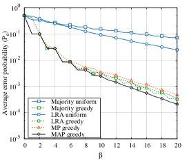
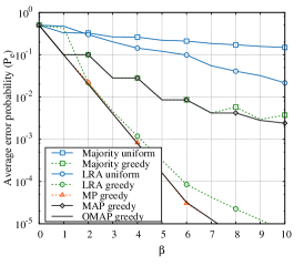
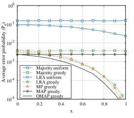
The first set of results is reported in Figures 1(a), 1(b),  1(c), and 2. For starters, results in these figures refer to the most classical scenario, where all tasks are identical. For what concerns workers, we define three classes, and the number of available workers per class is set to $W_{1}=30,W_{2}=120,W_{3}=150$. Since each worker can handle up to 20 tasks ($r_{w}=20$), the maximum number of assignments that can be handled by the three classes are 600, 2400, and 3000, respectively.

We set $\pi_{t1}=0.1,\pi_{t2}=0.2,\pi_{t3}=0.5$ for all $t$. This means that workers in class 1 are the most reliable, while workers in class 3 are spammers. This situation is summarized in Table I as Scenario 1.

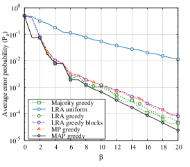
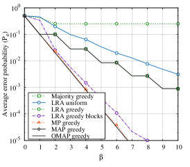
The results depicted in Figure 1(a) assume that all workers belonging to the same class have the same error probability i.e., $p_{tw}=\pi_{t,k(w)}$, $k(w)$ being the class worker $w$ belongs to. In particular, the figure shows the average task error probability, plotted versus the average number of workers per task, $\beta=C/T$. As expected, greedy allocation strategies perform much better due to the fact that they exploit the knowledge about the workers’ reliability ($p_{tw}$), and thus they assign tasks to the best possible performing workers. These strategies provide quite a significant reduction of the error probability, for a given number of workers per task, or a reduction in the number of assignments required to achieve a fixed target error probability. For example, $P_{e}=10^{-2}$ can be achieved by greedy algorithms by assigning only 6 workers per task (on average), while algorithms unaware of workers reliability require significantly more than 20 workers per task (on average).

Since class 1 can handle up to 600 assignments, for the greedy allocation algorithm, and for $\beta>6$ the requester has to allocate tasks to workers of class 2 as well. Since workers of class 2 are less reliable than workers of class 1 the slopes of the curves decrease. This behavior is not shown by algorithms employing uniform allocation since they choose workers irrespectively of the class they belong to.

We also observe that: i) in this scenario the simple MAP decision rule is optimal (it perfectly coincides with the OMAP) ii) every decision rule (even the simple majority rule) when applied in conjunction with a greedy scheduler provides comparable performance with respect to the optimal MAP algorithm (within a factor 2), iii) the performance of the MP greedy algorithm is slightly worse than LRA greedy in this scenario; iv) some of the algorithms such as the “Majority greedy” exhibit a non monotonic behavior with respect to $\beta$; this is a consequence of the fact that in order to provide best performance, these schemes require the number of workers assigned to tasks to be odd.

As final remark, we would like to observe that we have also implemented the MP algorithm proposed in [6], obtaining in all cases results that are practically indistinguishable from LRA.

Next, we take into account the case where in each class workers do not behave exactly the same. As already observed, this may reflect both possible inaccuracies/errors in the reconstruction of user profiles, and the fact that the behavior of workers is not fully predictable, since it may vary over time. Specifically, we assume that, in each class, two types of workers coexist, each characterized by a different error probability $p_{tw}$. More precisely, workers of type 1 have error probability $p_{tw}=(1-x)\pi_{tk}$, while workers of type 2 have error probability probability $p_{tw}=(1-x)\pi_{tk}+x/2$, where $0\leq x\leq 1$ is a parameter. Moreover, workers are of type 1 and type 2 with probability $1-2\pi_{tk}$ and $2\pi_{tk}$, respectively, so that the average error probability over the workers in class $k$ is $\pi_{tk}$. This bimodal worker model, even if it may appear somehow artificial, is attractive for the following two reasons: i) it is simple (it depends on a single scalar parameter $x$), and ii) it encompasses as particular cases the two extreme cases of full knowledge and hammer-spammer. We would like to remark that the allocation algorithm is unaware of this bimodal behavior of the workers. Indeed, it assumes that all workers within class $k$ have the same error probability, $\pi_{tk}$.

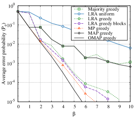
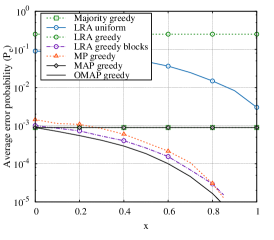
For $x=0$ all workers in each class behave exactly the same (they all have error probability $p_{tw}=\pi_{tk(w)}$); this is the case depicted in Figure 1(a). For $x=1$ we recover the hammer-spammer scenario; this case is represented in Figure 1(b), where workers are spammers with probability $2\pi_{tk}$ and hammers with probability $1-2\pi_{tk}$. Here, strategies employing the greedy allocation still greatly outperform schemes employing uniform allocations. However, differently from the previous case, the performance of the MAP decision rule is significantly sub-optimal in this scenario, when compared to “LRA greedy“, and “MP greedy”. This is due to the following two facts: i) MAP adopts a mismatched value of the error probability of individual workers, when $x\neq 0$, ii) MAP does not exploit the extra information on individual worker reliability that is possible to gather by jointly decoding different tasks. Observe that the performance of “LRA greedy“ and “MP greedy’ is not significantly different from OMAP. In particular the scheme “MP greedy” provides performance practically indistinguishable from OMAP in this scenario.

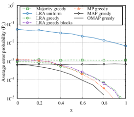
In Figure 1(c), for $\beta=10$, we show the error probability plotted versus the parameter $x$. We observe that the performance of the “MAP greedy” strategy is independent on the parameter $x$ while the performance of “LRA greedy” and “MP greedy” improves as $x$ increases. This effect can be explained by observing that the ability of distinguishing good performing workers from bad performing workers within the same class increases as $x$ increases. Observe also that the error probability achieved by “LRA greedy” and “MP greedy” is within a factor 2 from OMAP for every $x$. In particular, observe that for small values of $x$ the simple MAP decision rule represents a low-cost good performing decision strategy, but, as $x$ increases (i.e. the degree of heterogeneity increases within each class), more sophisticated decision rules which jointly decode large groups of tasks are needed to achieve good performance. It is worth observing that the performance of the “MP greedy” algorithm becomes very close to OMAP for large values of $x$.

In light of the previous observations, we can conclude that the a-priori information about worker reliability can be effectively exploited to improve the overall performance of the system both at the scheduler level (e.g. greedy vs uniform schemes) and at the decision rule level (e.g. “MAP” vs “Majority greedy” for small $x$ and “MP greedy” vs “LRA greedy” for large $x$).

Figure 2: Average error probability versus $\beta$ for different values of $T$

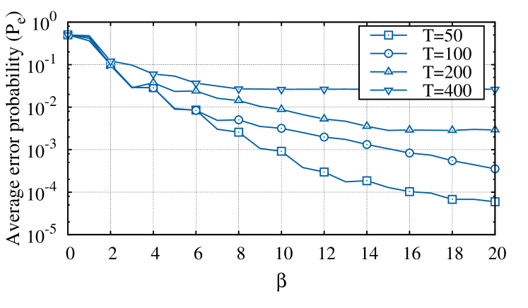
In Figure 2 we show the performance of the “LRA greedy” algorithm as the number of tasks varies while the pool of workers is the same as in the previous figures. Clearly, as the number of tasks increases the error probability increases since a larger amount of work is conferred to workers of classes 2 and 3. By looking at the curve for $T=200$ we observe that (i) for $0\leq\beta\leq 3$ only workers of class 1 are used; (ii) for $3<\beta\leq 15$ the slope of the curve decreases since workers of both classes 1 and 2 are used; (iii) for $\beta>15$ the requester allocates tasks also to workers of class 3 which are spammers. Therefore for $\beta>15$ the error probability does not further decrease.

VI-B Scenario 2

Figure 3: Scenario 2. Figures (a) and (b) report the average error probability versus the average number of workers per task, $\beta$, for $x=0$ and $x=1$, respectively. Figure (c) shows the average error probability versus $x$ and for $\beta=10$. The parameters of Scenario 2 are reported in Table I.

Next, we assume that the $T=100$ tasks are divided into 2 groups of 50 each. Workers processing tasks of group 1 and 2 are characterized by average error probabilities $\pi_{t1}=0.05,\pi_{t2}=0.1,\pi_{t3}=0.5$ and $\pi_{t1}=0.1,\pi_{t2}=0.2,\pi_{t3}=0.5$, respectively. This scenario reflects the case where tasks of group 2 are more difficult to solve than tasks of group 1 (error probabilities are higher). Workers of class ${\mathcal{C}}_{3}$ are spammers for both kinds of tasks. This situation is summarized in Table I as Scenario 2. Two different approaches are possible while applying LRA to scenario 2: i) we can independently apply LRA to blocks of indistinguishable tasks (we denote this strategy with “LRA greedy blocks”) placing ourselves on the safer side. ii) we can embrace a more risky approach by applying directly LRA to the whole set of tasks (we denote this strategy with “LRA greedy”). Regarding the MP decision algorithm, we have applied two independent instances of the algorithm to the two groups of tasks. The error probabilities provided by the considered algorithms are plotted in Figures 3(a),  3(b), and 3(c). For the sake of figure readability results of the basic “Majority uniform” strategy are not reported. First, observe that the relative ranking of all strategies is essentially not varied with respect to Scenario 1. In particular, we wish to highlight the significant performance gain exhibited by strategies employing the greedy allocation strategy over those employing a uniform allocation, such as “LRA uniform“. Second, observe that at first glance unexpectedly the “LRA greedy” slightly outperforms “LRA greedy blocks” for small $x$. This should not be too surprising, in light of the fact that: i) even if the error probability of each user depends on the specific task, the relative ranking among workers remains the same for all tasks, ii) ‘LRA greedy” gets advantage from the fact that all tasks are jointly decoded (i.e. SVD decomposition is applied to a larger matrix ${\bf A}$ better filtering out noise).

VI-C Scenario 3

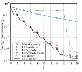
Finally, in Figures 4(a),  4(b), and 4(c) we consider a third scenario in which again tasks are partitioned into two groups of 50 each. Here, however, the number of available workers per class is set to $W_{1}=40,W_{2}=120,W_{3}=40$, and the workers error probabilities for the tasks in group 1 and 2 are given by $\pi_{t1}=0.1,\pi_{t2}=0.25,\pi_{t3}=0.5$, and $\pi_{t1}=0.5,\pi_{t2}=0.25,\pi_{t3}=0.1$, respectively. This situation reflects the case where workers are more specialized or interested in solving some kinds of tasks. More specifically, here workers of class 1 (class 3) are reliable when processing tasks of group 1 (group 2), and behave as spammers when processing tasks of group 2 (group 1). Workers of class 2 behave the same for all tasks. This situation is summarized in Table I as Scenario 3. We remark that, as in Scenario 2, we have applied two independent instances of the MP decision algorithm to the two groups of tasks. In terms of performance, first observe that, also for this scenario, even a fairly imprecise characterization of the worker behavior can be effectively exploited by the requester to significantly improve system performance. Second observe that the “LRA greedy” algorithm shows severely degraded error probabilities for $\beta\leq 16$, while the “LRA greedy blocks” (which we recall applies LRA independently to the two blocks of indistinguishable tasks) behaves properly. The behavior of “LRA greedy” should not surprise the reader, since our third scenario may be considered as possibly adversarial for the LRA scheme (when applied carelessly), in light of the fact that the relative ranking among workers heavily depends on the specific task. Nevertheless, it may still appear amazing that “LRA greedy” behaves even worse than the “LRA uniform” scheme in several cases. The technical reason for this behavior is related to the fact that, in our example, for $\beta\leq 16$, tasks of group 1 (group 2) are allocated to workers of class 1 (class 3) only, whilst workers of class 2 are not assigned any task. Instead, for $16<\beta\leq 20$ tasks of both types are also allocated to workers of class 2. This situation is summarized in Table II where $d_{tk}^{(i)}$ represents the number of times a task of type $i$ is assigned to workers of class $k$.

TABLE II: Assignments per task for Scenario 3 as a function of $\beta$

	$d_{t1}^{(1)}$	$d_{t1}^{(2)}$	$d_{t2}^{(1)}$	$d_{t2}^{(2)}$	$d_{t3}^{(1)}$	$d_{t3}^{(2)}$
$\beta\mathord{\leq}16$	$\beta$	0	0	0	0	$\beta$
$16\mathord{<}\beta\mathord{\leq}20$	$\beta$	0	$\beta\mathord{-}16$	$\beta\mathord{-}16$	0	$\beta$

For this reason, when $\beta\leq 16$ the matrix ${\bf A}$ turns out to have a block diagonal structure, which conflicts with the basic assumption made by LRA that matrix $\mathbb{E}[{\bf A}]$ can be well approximated by a rank-1 matrix.

It follows that the rank-1 approximations are extremely inaccurate when applied to the whole matrix ${\bf A}$ and thus provide high error probabilities. In such situations, by applying the LRA algorithm separately on each block of tasks (under the assumption that we have enough a-priori information to partitioning tasks into groups), we achieve huge performance gains.

Figure 4: Scenario 3. Figures (a) and (b) report the average error probability versus the average number of workers per task, $\beta$, for $x=0$ and $x=1$, respectively. Figure (c) shows the average error probability versus $x$ and for $\beta=10$. The parameters of Scenario 3 are reported in Table I.

Finally, we want to remark that we have tested several versions of greedy algorithms under different objective functions, such as $\Phi_{1}({\mathcal{G}})$, $\Phi_{2}({\mathcal{G}})$, and $\Phi_{3}({\mathcal{G}})$, finding that they provide, in general, comparable performance. The version employing mutual information was often providing slightly better results, especially in the case of LRA greedy and MP greedy. This can be attributed to the following two facts: i) the mutual information was proved to be submodular; ii) being mutual information independent from the adopted decoding scheme, it provides a more reliable metric for comparing the performance of different task allocations under the LRA decoding scheme with respect to the error probability $\Phi_{1}({\mathcal{G}})$ (which, we recall, is computed under the assumption that the decoding scheme is MAP). Unfortunately, due to the lack of space, we cannot include these results in the paper.

VI-D Scenario 4

Now, we move to a different scenario in which $T=100$ identical tasks are assigned to a population of 90 workers, each one characterized by an individual reliability index $p_{t,w}$. $p_{t,w}$ are uniformly and interdependently extracted in the range $(0,1/2]$. Parameters $p_{t,w}$ are assumed, in general, to be unknown to the system, which possesses just noisy estimates $\hat{p}_{t,w}$ of them. Such estimates are typically inferred from the analysis of past behavior of each worker, as better explained in the following. On the basis of $\hat{p}_{t,w}$, workers are grouped into $K$ classes. Specifically, classes are obtained by uniformly partitioning the interval $[0,1/2]$ in $K$ subintervals and assigning to class $k\in\{1,2,\cdots K\}$ all the workers whose estimated reliability index (error probability) $\hat{p}_{t,w}$ falls in the range $(\frac{k-1}{2K},\frac{k}{2K}]$. Then, the nominal error probability $\pi_{tk}$ assigned to class $k$, is set equal to the median point of he considered interval, i.e., $\pi_{tk}=\frac{2k-1}{4K}$.

Fig 5 reports the error probability achieved by the LRA-greedy algorithm vs $\beta$ for different values of $K$ in a optimistic scenario, in which perfect estimates of reliability indices are known to the system, i.e., $\hat{p}_{t,w}=p_{t,w}$.

As expected, by increasing $K$, a reduction of the error probability is observed. However note that performance improvements are significant only for relatively small values of $K$ and $\beta$. The marginal performance gain observed by increasing $K$ from 6 to 9, is rather limited for all values of $\beta$. Even in this ideal case in which full information on workers’ characteristics is available to the systems, scheduling tasks just on the basis of a rough classification of the workers into few classes is not particularly penalizing! These results, therefore, provide an empirical justification of our approach of partitioning users into few classes.

To complement previous results, Fig. 6 reports the error probability for specific values of $\beta$ and $K=6$ when the reliability estimate $\hat{p}_{t,w}$ is noisy. To keep things simple, we assume that all workers are tested on an initial number of tasks (called training tasks) and $\hat{p}_{t,w}$ is derived accordingly, as the empirical estimate of $p_{t,w}$ on the training tasks. However, we wish to remark that $\hat{p}_{t,w}$ can be, in principle, obtained by analyzing answer of workers on previously assigned tasks without the necessity of subjecting workers to an initial training phase. Once again, we would like to highlight that a detailed investigation of how $\hat{p}_{t,w}$ can be obtained goes beyond the scope of this paper.

Observe that when the number of training task is 0, no information about $\hat{p}_{t,w}$ is available and, therefore, workers are assigned to classes at random. Instead, when the number of training tasks becomes arbitrarily large, the system can count on exact estimates of the workers reliability indices. i.e., $\hat{p}_{t,w}={p}_{t,w}$.

Figure 5: Average error probability as a function of the average number of workers per task, $\beta$, in Scenario 4.

Figure 6: Average error probability as a function of the number of training tasks in Scenario 4.

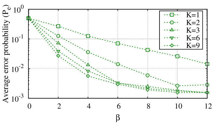
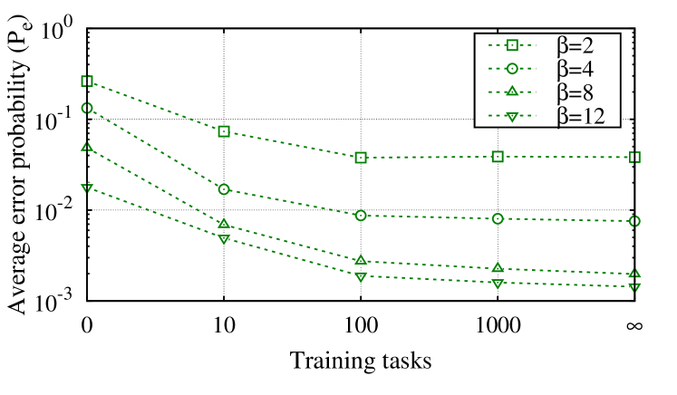
Figure  6 shows that even rather imprecise estimates of $\hat{p}_{t,w}$ (i.e., obtained through the analysis of relatively short sequences of training tasks) can be effectively exploited to significantly improve the performance of the system. Furthermore, observe that marginal gains significantly reduces as the length of training set increases. In particular, for moderate values of $\beta$, performance obtained when the training set size is set to 100 is hardly distinguishable from that observed when arbitrarily long training sets are employed. This provides further support to the viability of our approach, which appears rather robust to possibly imprecise estimates of workers’ reliability indices.

VII Concluding Remarks

In this paper we have presented the first systematic investigation of the impact of information about workers’ reputation in the assignment of tasks to workers in crowd work systems, quantifying the potential performance gains in several cases. We have formalized the optimal task assignment problem when workers’ reputation estimates are available, as the maximization of a monotone (submodular) function subject to Matroid constraints. Then, being the optimal problem NP-hard, we have proposed a simple but efficient greedy heuristic task allocation algorithm. We have also described a simple “maximum a-posteriori“ decision rule and a well-performing message-passing decision algorithm. We have tested our proposed algorithms, and compared them to different solutions, which can be obtained by extrapolating the proposals for the cases when reputation information is not available, showing that the crowd work system performance can greatly benefit from even largely inaccurate estimates of workers’ reputation. Our numerical results have shown that:

• even a significantly imperfect characterization of the workers’ reputation can be extremely useful to improve the system performance;

• the application of advanced joint task decoding schemes such as message passing can further improve the overall system performance, especially in the realistic case in which the a-priori information about worker reputation is largely affected by errors;

• the performance of advanced joint tasks decoding schemes such as LRA applied naively may become extremely poor in adversarial scenarios.

• the results show that “LRA greedy” and “MP greedy” algorithms perform well in most of the cases; their difference in terms of performance is rather limited, therefore they can both be used equivalently in a real-world scenario.

Future work directions include the extension to time-varying workers’ behavior, non-binary tasks, and the desing of effective algorithms for estimating workers’ error probability.

Appendix A Matroid definition and Proof of Proposition 3.1

First we recall the definition of a Matroid. Given a family $\mathbfcal F$ of subsets of a finite ground set ${\mathcal{O}}$ (i.e., $\mathbfcal F\subset 2^{{\mathcal{O}}})$, $\mathbfcal F$ is a Matroid iff: i) if ${\mathcal{G}}\in\mathbfcal F$, then ${\mathcal{H}}\in\mathbfcal F$ whenever ${\mathcal{H}}\subseteq{\mathcal{G}}$;
ii) if ${\mathcal{G}}\in\mathbfcal F$ and ${\mathcal{H}}\in\mathbfcal F$ with $|{\mathcal{G}}|>|{\mathcal{H}}|$, then there exists a $(t_{0},w_{0})\in{\mathcal{G}}\setminus{\mathcal{H}}$.

Now we can prove Proposition 3.1. First, observe that in our case property i) trivially holds. Then, we show that property ii) holds too. Given that $|{\mathcal{G}}|>|{\mathcal{H}}|$ and since by construction $|{\mathcal{G}}|=\sum_{w}{\mathcal{L}}(w,{\mathcal{G}})$ and $|{\mathcal{H}}|=\sum_{w}{\mathcal{L}}(w,{\mathcal{H}})$, necessarily there exists an $w_{0}$ such that $|{\mathcal{L}}(w_{0},{\mathcal{G}})|>|{\mathcal{L}}(w_{0},{\mathcal{H}})|$. This implies that ${\mathcal{L}}(w_{0},{\mathcal{G}})\setminus{\mathcal{L}}(w_{0},{\mathcal{H}})\neq\emptyset$. Let $(t_{0},w_{0})$ be an individual assignment in ${\mathcal{L}}(w_{0},{\mathcal{G}})\setminus{\mathcal{L}}(w_{0},{\mathcal{H}})$. Since by assumption $|{\mathcal{L}}(w_{0},{\mathcal{H}})|<|{\mathcal{L}}(w_{0},{\mathcal{G}})|\leq r_{w_{0}}$, denoted with ${\mathcal{H}}^{\prime}={\mathcal{H}}\cup\{(t_{0},w_{0})\}$, we have that $|{\mathcal{L}}(w_{0},{\mathcal{H}}^{\prime})|=|{\mathcal{L}}(w_{0},{\mathcal{H}})|+1\leq|{\mathcal{L}}(w_{0},{\mathcal{G}})|\leq r_{w_{0}}$ similarly $|{\mathcal{H}}^{\prime}|=|{\mathcal{H}}|+1\leq|{\mathcal{G}}|\leq C$, therefore ${\mathcal{H}}^{\prime}\in\mathbfcal F$.

The fact that in our case $q=\frac{\max_{{\mathcal{G}}in\mathbfcal B}|{\mathcal{G}}|}{\min_{{\mathcal{G}}in\mathbfcal B}|{\mathcal{G}}|}=1$ descends immediately by the fact that necessarily ${\mathcal{G}}\in\mathbfcal B$ iff either i) $|{\mathcal{G}}|=C$ when $C\leq\sum_{w}r_{w}$ or ii) $|{\mathcal{G}}|=\sum_{w}r_{w}$ when $C>\sum_{w}r_{w}$.

Appendix B Mutual information for known error probabilities $\pi_{tk}$

The workers’ answers about the tasks $\bm{\tau}$ are collected in the random $T\times W$ matrix ${\bf A}({\mathcal{G}})$, defined in Section II of the main document. The information that the answers ${\bf A}$ provide about the tasks $\bm{\tau}$ is denoted by

$$I({\bf A};\bm{\tau})=H({\bf A})-H({\bf A}|\bm{\tau})$$

where the entropy $H(a)$ and the conditional entropy $H(a|b)$ have been defined in Section III.C of the main document. We first compute $H({\bf A}|{\bf t})$ and we observe that, given the tasks $\bm{\tau}$, the answer ${\bf A}$ are independent, i.e., $\mathbb{P}\{{\bf A}|\bm{\tau}\}=\prod_{k=1}^{K}\prod_{t=1}^{T}\mathbb{P}\{{\bf a}_{tk}|\tau_{t}\}$, where ${\bf a}_{tk}$ is the vector of answers to task $\theta_{t}$ from users of class ${\mathcal{C}}_{k}$. Since $\mathbb{P}\{{\bf A}|\bm{\tau}\}$ has a product form, we obtain $H({\bf A}|\bm{\tau})=\sum_{k=1}^{K}\sum_{t=1}^{T}H({\bf a}_{tk}|\tau_{t})$. Thanks to the fact that workers of the same class are independent and all have error probability $\pi_{tk}$, we can write $H({\bf a}_{tk}|\tau_{t})=d_{ik}H_{b}(\pi_{k})$ where $H_{b}(p)=-p\log p-(1-p)\log(1-p)$ and $d_{tk}$ is the number of allocations of task $t$ in class ${\mathcal{C}}_{k}$. In conclusion, we get:

$$H({\bf A}|\bm{\tau})=\sum_{t=1}^{T}\sum_{k=1}^{K}d_{tk}H_{b}(\pi_{tk})$$

As for the entropy $H({\bf A})$, we have:

$$\mathbb{P}\{{\bf A}\}=\mathbb{E}_{\bm{\tau}}\mathbb{P}\{{\bf A}|\bm{\tau}\}=\mathbb{E}_{\bm{\tau}}\prod_{t=1}^{T}\mathbb{P}\{{\bf a}_{t}|\tau_{t}\}=\prod_{t=1}^{T}\mathbb{E}_{\tau_{t}}\mathbb{P}\{{\bf a}_{t}|\tau_{t}\}$$

where ${\bf a}_{t}$ is the vector of answers to task $\theta_{t}$ (corresponding to the $t$-th row of ${\bf A}$). Note that $\mathbb{E}_{\tau_{t}}\mathbb{P}\{{\bf a}_{t}|\tau_{t}\}=\mathbb{P}\{{\bf a}_{t}\}$, hence $\mathbb{P}\{{\bf A}\}=\prod_{t=1}^{T}\mathbb{P}\{{\bf a}_{t}\}$ and we immediately obtain $H({\bf A})=\sum_{t=1}^{T}H({\bf a}_{t})$. The probabilities $\mathbb{P}\{{\bf a}_{tk}|\tau_{t}=1\}$ and $\mathbb{P}\{{\bf a}_{tk}|\tau_{i}=-1\}$ are easy to compute. Indeed for $\tau_{t}=-1$ we have

$$\mathbb{P}\{{\bf a}_{tk}|\tau_{t}=-1\}=\pi_{tk}^{d_{tk}-m_{tk}}(1-\pi_{tk})^{m_{tk}}$$ (24)

where $m_{tk}$ is the number of “$-1$” answers to task $\theta_{t}$ from class-$k$ workers. The above formula derives from the fact that workers of the same class are independent and have the same error probability $\pi_{tk}$. Similarly

$$\mathbb{P}\{{\bf a}_{tk}|\tau_{t}=+1\}=\pi_{tk}^{m_{tk}}(1-\pi_{tk})^{d_{tk}-m_{tk}}$$ (25)

The expressions (24) and (25) can compactly written as

$$\mathbb{P}\{{\bf a}_{tk}|\tau_{t}\}=(1-\pi_{tk})^{d_{tk}}b_{tk}^{(1-\tau_{t})d_{tk}/2-m_{tk}\tau_{t}}$$ (26)

where $b_{tk}=\pi_{tk}/(1-\pi_{tk})$. Since, given $\tau_{t}$, workers are independent, we obtain

$$\mathbb{P}\{{\bf a}_{t}\} = \mathbb{E}_{\tau_{t}}\mathbb{P}\{{\bf a}_{t}|\tau_{t}\}$$

$$= \gamma_{tk}\mathbb{E}_{\tau_{t}}\left[\prod_{k=1}^{K}b_{tk}^{(1-\tau_{t})d_{tk}/2-m_{tk}\tau_{t}}\right]$$

$$= \frac{\gamma_{tk}}{2}\left[\prod_{k=1}^{K}b_{tk}^{-m_{tk}}+\prod_{k=1}^{K}b_{tk}^{d_{tk}+m_{tk}}\right]=\frac{\gamma_{tk}}{2}f({\bf m}_{t})$$

with ${\bf m}_{t}=[m_{t1},\ldots,m_{tK}]$ and $f({\bf h})=\prod_{k=1}^{K}b_{tk}^{-h_{k}}+\prod_{k=1}^{K}b_{tk}^{d_{tk}+h_{k}}$. Finally, by using the definition of entropy,

$$H({\bf a}_{t}) = \mathbb{E}_{{\bf a}_{t}}[-\log\mathbb{P}\{{\bf a}_{t}\}]$$

$$= -\log\frac{\gamma_{tk}}{2}-\mathbb{E}_{{\bf a}_{t}}f({\bf m}_{t})$$

$$= -\log\frac{\gamma_{tk}}{2}-\frac{\gamma_{tk}}{2}\sum_{{\bf n}}f({\bf n})\log f({\bf n})\prod_{k=1}^{K}\binom{m_{tk}}{n_{k}}$$

where ${\bf n}=[n_{1},\ldots,n_{K}]$ and $n_{k}=0,\ldots,m_{tk}$, $k=1,\ldots,K$. Note that the computation of (LABEL:eq:Hat) is exponential in the number of classes $K$.

Appendix C Submodularity of the mutual information

Let ${\mathcal{G}}_{1}$ and ${\mathcal{G}}_{2}$ be two generic allocations for task $\theta$, such that ${\mathcal{G}}_{2}\subseteq{\mathcal{G}}_{1}$ and ${\mathcal{G}}_{1}={\mathcal{G}}_{2}\cup{\mathcal{G}}_{3}$. Also let the pair $\gamma=(t,w)\in{\mathcal{O}}\setminus{\mathcal{G}}_{1}$. Let ${\bf a}({\mathcal{G}})$ be the random vector of answers corresponding to the allocation ${\mathcal{G}}$. For the sake of notation simplicity in the following we define ${\bf a}_{j}={\bf a}({\mathcal{G}}_{j})$, $j=1,2,3$, and $a_{\gamma}={\bf a}(\gamma)$ (since $\gamma$ is a single pair, the answer ${\bf a}(\gamma)$ is scalar).

Then the mutual information $I({\bf a}({\mathcal{G}});\tau)$ is submodular if

$$I({\bf a}({\mathcal{G}}_{2}\cup\gamma);\tau)-I({\bf a}_{2};\tau)\geq I({\bf a}({\mathcal{G}}_{1}\cup\gamma);\tau)-I({\bf a}_{1};\tau)\,.$$ (28)

We first observe that

$$I({\bf a}({\mathcal{G}}_{1}\cup\gamma);\tau) = I({\bf a}({\mathcal{G}}_{2}\cup{\mathcal{G}}_{3}\cup\gamma);\tau)$$

$$\stackrel{{\scriptstyle(a)}}{{=}} I({\bf a}_{2},{\bf a}_{3},a_{\gamma};\tau)$$

$$\stackrel{{\scriptstyle(b)}}{{=}} I({\bf a}_{2},a_{\gamma};\tau)+I({\bf a}_{3};\tau|{\bf a}_{2},a_{\gamma})$$

where in $(a)$ we exploited the fact that the sets ${\mathcal{G}}_{3}$, ${\mathcal{G}}_{2}$, and $\gamma$ are disjoint while in $(b)$ we applied the mutual information chain rule. Similarly we can write $I({\bf a}_{1};\tau)=I({\bf a}_{2};\tau)+I({\bf a}_{3};\tau|{\bf a}_{2})$ By consequence (28) reduces to

$$I({\bf a}_{3};\tau|{\bf a}_{2})\geq I({\bf a}_{3};\tau|{\bf a}_{2},a_{\gamma})$$

By applying to both sides of the above inequality the definition of the mutual information given in the main document, equation (7), we obtain

$$H({\bf a}_{3}|{\bf a}_{2})\mathord{-}H({\bf a}_{3}|\tau,{\bf a}_{2})\mathord{\geq}H({\bf a}_{3}|{\bf a}_{2},a_{\gamma})\mathord{-}H({\bf a}_{3}|\tau,{\bf a}_{2},a_{\gamma})$$ (29)

Since workers are independent we now observe that $H({\bf a}_{3}|\tau,{\bf a}_{2})=H({\bf a}_{3}|\tau)$ since ${\bf a}_{3}$ only depends on $\tau_{t}$. Therefore (29) reduces to

$$H({\bf a}_{3}|{\bf a}_{2})\geq H({\bf a}_{3}|{\bf a}_{2},a_{\gamma})$$

which holds due to the fact that entropy is reduced by conditioning.

Appendix D Derivation of equation (24) of the main document

In the $l$-th iteration of the MP algorithm, an updated pdf of the error probability of worker $w$, $p_{w}$, is computed given the answer matrix ${\bf A}$ and the current posterior probability distribution of task solutions, used as a-priori.

Let $\rho_{t}^{(l)}(\pm 1)$ be the posterior probability distribution for task $t$ at iteration $l$. Also, let $f_{k(w)}^{(0)}(p)$ be the a-priori distribution of the error probability for class $k(w)$ which worker $w$ belongs to. In the computation of the pdf $f_{tw}^{(l)}(p)$ of $p_{w}$, we use extrinsic information, i.e., we only use $\rho_{t^{\prime}}^{(l)}(\pm 1)$ for $t\neq t^{\prime}$. We have, thanks to Bayes’ rule, that

$$f_{tw}^{(l)}(p)\propto f_{k(w)}^{(0)}(p)\mathbb{P}\{{\bf A}|p_{w}=p,\{\rho_{t^{\prime}}^{(l)}(\pm 1)\}_{t^{\prime}\neq t}\}$$ (30)

where

$$\mathbb{P}\{{\bf A}|p_{w}\mathord{=}p,\{\rho_{t^{\prime}}^{(l)}(\pm 1)\}_{t^{\prime}\neq t}\}\mathord{\propto}\prod_{t^{\prime}\neq t}\mathbb{P}\{a_{t^{\prime}w}|p_{w}\mathord{=}p,\rho_{t^{\prime}}^{(l)}(\pm 1)\}$$ (31)

In both equations above, the omitted factors do not depend on $p$. Now

$$\begin{split}\mathbb{P}\{a_{tw}|p_{w}=p,&\rho_{t}^{(l)}(\pm 1)\}=\\ &\mathbb{P}\{a_{tw}|p_{w}=p,t=1\}\rho_{t}^{(l)}(1)\\ &+\mathbb{P}\{a_{tw}|p_{w}=p,t=-1\}\rho_{t}^{(l)}(-1)\end{split}$$ (32)

and

$$\mathbb{P}\{a_{tw}|p_{w}=p,t=\pm 1\}=\frac{1}{2}\left[1\pm(1-2p)a_{tw}\right]$$ (33)

Substituting back (33) into (32), we obtain

$$\begin{split}\mathbb{P}\{a_{tw}|p_{w}=p,&\rho_{t}^{(l)}(\pm 1)\}\\ &=\frac{1}{2}\left[1+(1-2p)a_{tw}\left(\rho_{t}^{(l)}(1)-\rho_{t}^{(l)}(-1)\right)\right]\end{split}$$ (34)

Finally, from the definition of LLR, we have

$$m_{t\rightarrow w}^{(l)}=\log\frac{\rho_{t}^{(l)}(1)}{\rho_{t}^{(l)}(-1)}$$ (35)

so that

$$\rho_{t}^{(l)}(1)=\frac{{\rm e}^{m_{t\rightarrow w}^{(l)}}}{1+{\rm e}^{m_{t\rightarrow w}^{(l)}}}$$ (36)

and

$$\rho_{t}^{(l)}(1)-\rho_{t}^{(l)}(-1)=\tanh\left(\frac{m_{t\rightarrow w}^{(l)}}{2}\right)$$ (37)

Substituting (37) into (34), and then back into (31) and (30), we obtain equation (24) appearing in the main document.

References

- [1] M.-C. Yuen, I. King, and K.-S. Leung, “A Survey of Crowdsourcing Systems,” IEEE PASSAT-SOCIALCOM, Boston (MA), USA, Oct. 9–11, pp. 766–773, 2011.
- [2] D. E. Difallah, M. Catasta, G. Demartini, P. G. Ipeirotis, and P. Cudré-Mauroux, “The dynamics of micro-task crowdsourcing: The case of amazon mturk”, Proceedings of the 24th International Conference on World Wide Web, pp. 238–247, 2015.
- [3] A. Kittur, J. V. Nickerson, M. Bernstein, E. Gerber, A. Shaw, J. Zimmerman, M. Lease, and J. Horton, “The future of crowd work,” ACM CSCW, San Antonio, Texas, USA, 2013.
- [4] E. Peer, J. Vosgerau, and A. Acquisti, “Reputation as a sufficient condition for data quality on Amazon Mechanical Turk,” Behavior Research Methods, v. 46, pp. 1023–1031.
- [5] D. R. Karger, S. Oh and D. Shah, “Budget- optimal Crowdsourcing Using Low-rank Matrix Approximations,” 49th Allerton Conf. on Communication, Control, and Computing, pp. 284–291, Sept. 28–30, 2011.
- [6] D. R. Karger, S. Oh, and D. Shah, ”Budget-Optimal Task Allocation for Reliable Crowdsourcing Systems,” Operations Research, Vol. 62, No. 1, pp. 1–24, 2014.
- [7] D. R. Karger, S. Oh, and D. Shah, ”Efficient crowdsourcing for multi-class labeling,” SIGMETRICS Perform. Eval. Rev., Vol. 41, No. 1, pp. 81–92, June 2013.
- [8] A. Ghosh, S. Kale, and P. McAfee, “Who moderates the moderators?: crowdsourcing abuse detection in user-generated content,” 12th ACM Conf. on Electronic commerce, New York, NY, USA, pp. 167–176, 2011.
- [9] I. Abraham, O. Alonso, V. Kandylas, and A. Slivkins, ”Adaptive Crowdsourcing Algorithms for the Bandit Survey Problem,” http://arxiv.org/abs/1302.3268.
- [10] H. Zhang, Y. Ma, and M. Sugiyama, “Bandit-based task assignment for heterogeneous crowdsourcing”, Neural computation, 2015.
- [11] Y. Zheng, J. Wang, G. Li, R. Cheng, and J. Feng, “QASCA: a quality-aware task assignment system for crowdsourcing applications”, Proceedings of the 2015 ACM SIGMOD International Conference on Management of Data, pp. 1031-1046, 2015.
- [12] Y. Bachrach, T. Graepel, T. Minka, and J. Guiver, “How To Grade a Test Without Knowing the Answers–A Bayesian Graphical Model for Adaptive Crowdsourcing and Aptitude Testing”, ArXiv Preprint, arXiv:1206.6386, 2012.
- [13] V. C. Raykar, S. Yu, L. H. Zhao, G. H. Valadez, C. Florin, L. Bogoni, and L. Moy, “Learning from crowds”, the Journal of Machine Learning Research, v. 11, pp. 1297–-1322, 2010.
- [14] D. Lee, J. Kim, H. Lee, and K. Jung, “Reliable Multiple-choice Iterative Algorithm for CS Systems”, in Proc. of the 2015 ACM SIGMETRICS International Conference on Measurement and Modeling of Computer Systems, pp. 205–216, 2015.
- [15] J. Whitehill, T.-f. Wu, J. Bergsma, J. R. Movellan, and P. L. Ruvolo, “Whose vote should count more: Optimal integration of labels from labelers of unknown expertise”, Advances in neural information processing systems, pp. 2035–-2043, 2009.
- [16] S. Kerr, “On the folly of rewarding A, while hoping for B”, Academy of Management Journal, pp. 769–783, 1975.
- [17] D. Chandler, and A. Kapelner, “Breaking monotony with meaning: Motivation in crowdsourcing markets”, Journal of Economic Behavior & Organization, pp. 123-133, 2013.
- [18] A. Kittur, E.H. Chi, and B. Suh, “Crowdsourcing user studies with Mechanical Turk”, Proceedings of the 26th annual SIGCHI conference on Human factors in computing systems - CHI ’08, pp. 453–456, 2008.
- [19] S. Lewis, M. Dontcheva, and E. Gerber, “Affective computational priming and creativity”, Proceedings of the 2011 annual conference on Human factors in computing systems - CHI’ 11, pp. 735–744, 2011.
- [20] W. Mason, and D.J. Watts, “Financial Incentives and the Performance of Crowds”, Proceedings of The ACM Conference on Human Computation & Crowdsourcing 2009, 2009.
- [21] J. Rogstadius, V. Kostakos, A. Kittur, B. Smus, J. Laredo, and M. Vukovic, “An Assessment of Intrinsic and Extrinsic Motivation on Task Performance in Crowdsourcing Markets”, Proceedings of the Fifth International AAAI Conference on Weblogs and Social Media, 2011.
- [22] A.D. Shaw, J.J., Horton, and D.L. Chen, “Designing incentives for inexpert human raters”, Proceedings of the ACM 2011 conference on Computer supported cooperative work, pp. 275–284, 2011.
- [23] C. J. Ho, A. Slivkins, S. Suri, and J. W. Vaughan, “Incentivizing high quality crowdwork”, Proceedings of the 24th International Conference on World Wide Web, pp. 419–429, 2015.
- [24] E. Christoforou, A. Fernandez Anta, C. Georgiou, M. A. Mosteiro, and A. Sanchez, “Applying the dynamics of evolution to achieve reliability in master-worker computing,” Concurrency and Computation: Practice and Experience Vol. 25, No. 17, pp. 2363–2380, 2013.
- [25] A. Fernandez Anta, C. Georgiou, and M. A. Mosteiro, “Algorithmic mechanisms for internet-based master-worker computing with untrusted and selfish workers,” IEEE IPDPS 2010, Atlanta (GA), April 2010.
- [26] A. Fernandez Anta, C. Georgiou, L. Lopez, and A. Santos, “Reliable internet-based master-worker computing in the presence of malicious workers,” Parallel Processing Letters, Vol. 22, No. 1, 2012.
- [27] A. Singla and A. Krause, “Truthful incentives in crowdsourcing tasks using regret minimization mechanisms,” 22nd international conference on World Wide Web, Rio de Janeiro, Brazil, May 2013.
- [28] E. Kamar and E. Horvitz, ”Incentives for truthful reporting in crowdsourcing,” 11th International Conference on Autonomous Agents and Multiagent Systems, Valencia, ES, pp. 1329-1330, June 2012.
- [29] P. Donmez, J. G. Carbonell, and J. Schneider, “Efficiently learning the accuracy of labeling sources for selective sampling,” 15th ACM SIGKDD international conference on Knowledge discovery and data mining, New York (NY), USA, pp. 259-268, June 2009.
- [30] Y. Zheng, S. Scott, and K. Deng, “Active learning from multiple noisy labelers with varied costs,” 2010 IEEE 10th International Conference on Data Mining, Sydney, Australia, Dec. 13–17, pp. 639–648, 2010.
- [31] E. Christoforou, A. Fernández Anta, C. Georgiou, M. A. Mosteiro, “Reputation-Based Mechanisms for Evolutionary Master-Worker Computing,” in Principles of Distributed Systems: Proc. of the 17th International Conference, OPODIS 2013, Nice, France, pp. 98–113, 2013.
- [32] U. Gadiraju, R. Kawase, S. Dietze, and G. Demartini, “Understanding malicious behavior in crowdsourcing platforms: The case of online surveys”, Proceedings of CHI, 2015.
- [33] M. Kokkodis, and P. G. Ipeirotis, “Reputation Transferability in Online Labor Markets”, Management Science, 2015.
- [34] J. Fan, G. Li, B. C. Ooi, K. L. Tan, and J. Feng, “iCrowd: An Adaptive CS Framework”, Proceedings of the 2015 ACM SIGMOD International Conference on Management of Data, pp. 1015–1030, 2015.
- [35] J.M. Rzeszotarski, and A. Kittur, “Instrumenting the crowd: using implicit behavioral measures to predict task performance”, Symposium on User Interface Software and Technology - UIST ’11, 2011.
- [36] J.M. Rzeszotarski, and A. Kittur, “CrowdScape: interactively visualizing user behavior and output”, Proc. of the 25th annual ACM symposium on User interface software and technology - UIST ’12, pp. 55–-62, 2012.
- [37] R. Buettner, “A Systematic Literature Review of CS Research from a Human Resource Management Perspective”, IEEE 48th Hawaii International Conference on System Sciences (HICSS), pp. 4609–4618, 2015.
- [38] A. Tarable, A. Nordio, E. Leonardi, and M. Ajmone Marsan, “The Importance of Being Earnest in Crowdsourcing Systems”, IEEE INFOCOM, Hong Kong, April 2015.
- [39] T. M. Cover and J. M. Thomas, “Elements of information theory,” 2nd ed., John Wiley, 2005.
- [40] G. Calinescu, C. Chekuri, M. Pál, J. Vondrák, “Maximizing a Monotone Submodular Function Subject to a Matroid Constraint,” SIAM Journal on Computing, Vol. 40, No. 6, pp. 1740–1766, 2011.