Elasticity of a semiflexible filament with a discontinuous tension due to a cross-link or a molecular motor

Mohammadhosein Razbin1 m.razbin@theorie.physik.uni-goettingen.de    Panayotis Benetatos2 pben@knu.ac.kr    Annette Zippelius1 1 Institute for Theoretical Physics, Georg August University, Friedrich-Hund-Platz 1, 37077 Göttingen, Germany
2 Department of Physics, Kyungpook National University, 80 Daehakro, Bukgu, Daegu 702-701, Republic of Korea
(Published in Physical Review E (18 May 2016))
Abstract

We analyze the stretching elasticity of a wormlike chain with a tension discontinuity resulting from a Hookean spring connecting its backbone to a fixed point. The elasticity of isolated semiflexible filaments has been the subject in a significant body of literature, primarily because of its relevance to the mechanics of biological matter. In real systems, however, these filaments are usually part of supramolecular structures involving cross-linkers or molecular motors which cause tension discontinuities. Our model is intended as a minimal structural element incorporating such a discontinuity. We obtain analytical results in the weakly bending limit of the filament, concerning its force-extension relation and the response of the two parts in which the filament is divided by the spring. For a small tension discontinuity, the linear response of the filament extension to this discontinuity strongly depends on the external tension. For large external tension f𝑓f, the spring force contributes a subdominant correction 1/f3/2similar-toabsent1superscript𝑓32\sim 1/f^{3/2} to the well known 1/fsimilar-toabsent1𝑓\sim 1/\sqrt{f} dependence of the end-to-end extension.

pacs:
87.15.ad,87.80.Nj,87.16.ad,36.20.Ey
preprint: APS/123-QED

I Introduction

Over the past couple of decades, it has become clear that mechanics plays a very important role in the biological function of the cell, on a par with biochemistry Discher_Cell2006 ; Butcher_cancer_Nature2009 ; Ingber_Mechanics_Development2010 . In order to unravel the physical basis of the complex mechanical behaviour of biological matter, a bottom-up strategy has proven very fruitful bausch2006bottom . In this approach, the basic functional modules of the cytoskeleton are reconstituted in vitro and analysed experimentally in tandem with theoretical modelling.

The basic structural elements of the cytoskeleton (microtubules, intermediate filaments, F-actin) are all semiflexible polymers with a behaviour intermediate between that of a random coil and a rigid rod Terentjev_SM_review ; Broedersz_MacKintosh_RMP . They form supramolecular assemblies (e.g. networks, bundles) through cross-linking Bausch_Claessens_SM_review . Cross-linking involves a host of different filament-binding proteins Ayscough_ABPs ; Mandelkow_MAPs . Active processes in the cell, such as the delivery of cargos, transport of organelles, mitotic dynamics, as well as muscle contraction are carried out by molecular motors using actin filaments or microtubules as tracks. The bottom-up approach to the study of molecular motors aims at analysing the transduction of metabolic energy into mechanical force and motion at the microscopic level using in vitro assays Veigel_Schmidt_NR2011 . The advances in single-molecule manipulation are harnessed to study the simplest motor-filament complexes. In gliding assays, the motor (myosin, kinesin, or dynein) is attached to a glass surface and the translocation of the filament (F-actin or microtubule) is observed. In single motor assays, the filament is attached to the glass surface and the movement of the motor is monitored. In motor assays with beads, the motor is attached to a micron-sized refractile bead whose position is measured Holzbaur_Goldman_2010 .

In this paper, we investigate analytically the mechanical response of a semiflexible filament with a tension discontinuity. Our model system can be viewed as one of the simplest structural elements of the cytoskeleton beyond the isolated single-molecule level. We consider a semiflexible polymer, modelled as a wormlike chain, in the weakly bending approximation. The latter can be satisfied either by applying a strong tensile force which irons out large thermal undulations, or by having a filament with large persistence length compared to its contour length. A longitudinal Hookean spring whose one end is attached to a fixed substrate, has its other end on the filament thus exerting a force which causes the tension discontinuity. The position of one end of the filament is held fixed, whereas that of the other end fluctuates. Its average position yields the force-extension relations which are the main subject of our analysis. The spring may be viewed as representing a motor, according to the myosin cross-bridge model first introduced by Huxley in 1957 Huxley_1957 and still in use Guerin_Prost_Martin_Joanny . Our results apply to passive motors or to very slowly stepping motors, slower than the relaxation time of the filament. The time scale can be tuned by adjusting the concentration of ATP molecules. We should point out, however, that our study of semiflexible filaments with tension discontinuity is also relevant to passive cross-linkers of large size or compliance. Many of the actin binding proteins fall in this category as they can have large spacer domains Bausch_Claessens_SM_review

Our paper is organised as follows. In Sec. II we introduce the model and show how the discontinuity along the filament contour arises. In Sec. III we discuss the method of Green functions which allows us to calculate correlation functions of the filament tangent vector and therefore the force-extension relation for different boundary conditions. Explicit results for the case of small spring force, large spring force, and large spring and external forces with a small difference between them are given in Sec. IV. In Sec. V we discuss the relation of our analysis to single motor experiments. We conclude in Sec. VI, and details of our calculations are given in the Appendices.

II Model description

Our starting point is the wormlike chain model for a semiflexible filament of contour length L𝐿L which is attached to a point or wall on one side and pulled by a constant force, 𝐟𝐞𝐱𝐭subscript𝐟𝐞𝐱𝐭\mathbf{f_{ext}}, on the other side. Its Hamiltonian is given by

HWLC=κ20L(d𝐭ds)2𝐟𝐞𝐱𝐭0Ld𝐭dssubscript𝐻𝑊𝐿𝐶𝜅2superscriptsubscript0𝐿superscript𝑑𝐭𝑑𝑠2subscript𝐟𝐞𝐱𝐭superscriptsubscript0𝐿𝑑𝐭𝑑𝑠H_{WLC}=\frac{\kappa}{2}\int_{0}^{L}(\frac{d\mathbf{t}}{ds})^{2}-\mathbf{f_{ext}}\int_{0}^{L}\frac{d\mathbf{t}}{ds} (1)

Here 𝐭(s)𝐭𝑠\mathbf{t}(s) is the tangent vector at arclength s,0sL𝑠0𝑠𝐿s,0\leq s\leq L and κ𝜅\kappa denotes the bending stiffness. We will treat the above model in the weakly bending approximation Marko_Siggia , assuming that the persistence length lp=κ/(kBT)subscript𝑙𝑝𝜅subscript𝑘𝐵𝑇l_{p}=\kappa/(k_{B}T) is much larger than the length L𝐿L of the filament.

In the Monge parametrization PhysRevE.74.041803 , the tangent of a semiflexible filament is given by t(s)=11+a12(s)+a22(s)(1,a1(s),a2(s))𝑡𝑠11superscriptsubscript𝑎12𝑠superscriptsubscript𝑎22𝑠1subscript𝑎1𝑠subscript𝑎2𝑠t(s)=\frac{1}{\sqrt{1+a_{1}^{2}(s)+a_{2}^{2}(s)}}(1,a_{1}(s),a_{2}(s)). We assume that the filament is oriented along the x-direction, either due to the grafting on the left side and/or the pulling force 𝐟𝐞𝐱𝐭=fext𝐞xsubscript𝐟𝐞𝐱𝐭subscript𝑓𝑒𝑥𝑡subscript𝐞𝑥\mathbf{f_{ext}}=f_{ext}\mathbf{e}_{x}. In the weakly bending limit the transverse components of the tangent vector a1(s)subscript𝑎1𝑠a_{1}(s) and a2(s)subscript𝑎2𝑠a_{2}(s) are small. We therefore approximate tx(s)=112[a12(s)+a22(s)]subscript𝑡𝑥𝑠112delimited-[]superscriptsubscript𝑎12𝑠superscriptsubscript𝑎22𝑠t_{x}(s)=1-\frac{1}{2}[a_{1}^{2}(s)+a_{2}^{2}(s)] and (dt(s)ds)2=a˙12(s)+a˙22(s)superscript𝑑𝑡𝑠𝑑𝑠2subscriptsuperscript˙𝑎21𝑠subscriptsuperscript˙𝑎22𝑠(\frac{dt(s)}{ds})^{2}=\dot{a}^{2}_{1}(s)+\dot{a}^{2}_{2}(s) where the dot denotes the derivative with respect to s𝑠s. The Hamiltonan then reads

HWB=i=12[0L(κ2a˙i2(s)+fext2ai2(s))𝑑s]subscript𝐻𝑊𝐵superscriptsubscript𝑖12delimited-[]superscriptsubscript0𝐿𝜅2subscriptsuperscript˙𝑎2𝑖𝑠subscript𝑓𝑒𝑥𝑡2superscriptsubscript𝑎𝑖2𝑠differential-d𝑠H_{WB}=\sum_{i=1}^{2}\left[\int_{0}^{L}\left(\frac{\kappa}{2}\dot{a}^{2}_{i}(s)+\frac{f_{ext}}{2}a_{i}^{2}(s)\right)ds\right] (2)
Refer to caption
Refer to caption
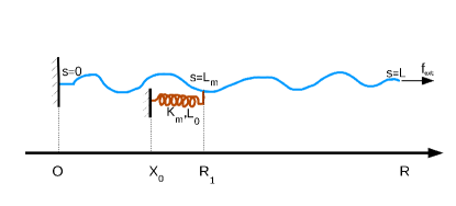
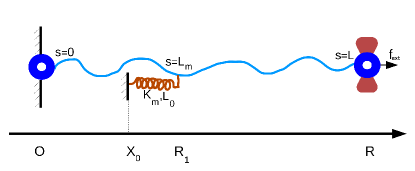
Figure 1: Schematic presentation of a filament attached to a spring with clamped-free and hinged-hinged boundary conditions at the ends. One end of the spring is fixed to the substrate. The spring pulls one side of the filament and pushes the other side. Therefore, the two sides of the filament are at different tension.

Here, we are interested in the effects of a motor whose one end is grafted to a substrate while the other end is attached to the filament at arclength Lmsubscript𝐿𝑚L_{m}. In the simplest model, the motor is just a spring of rest length L0subscript𝐿0L_{0}. and spring constant kmsubscript𝑘𝑚k_{m}

Hspring=km2(R1X0L0)2subscript𝐻𝑠𝑝𝑟𝑖𝑛𝑔subscript𝑘𝑚2superscriptsubscript𝑅1subscript𝑋0subscript𝐿02H_{spring}=\frac{k_{m}}{2}(R_{1}-X_{0}-L_{0})^{2} (3)

When the motor steps along the filament, its effective spring is compressed or extended beyond the rest length, resulting in a force, fmsubscript𝑓𝑚f_{m} on the filament. Since the pulling force, fextsubscript𝑓𝑒𝑥𝑡f_{ext}, is fixed the presence of the motor will result in a compression or extension of the filament. In this paper, we compute the change in the force-extension relation of the filament due to the attached motor.

In the weakly bending approximation, we can represent the total Hamiltonian H=HWB+Hspring𝐻subscript𝐻𝑊𝐵subscript𝐻𝑠𝑝𝑟𝑖𝑛𝑔H=H_{WB}+H_{spring} in the form of a filament with an arclength dependent tension:

H=i=12[0L(κ2a˙i2(s)+f(s)2ai2(s))𝑑s]𝐻superscriptsubscript𝑖12delimited-[]superscriptsubscript0𝐿𝜅2subscriptsuperscript˙𝑎2𝑖𝑠𝑓𝑠2superscriptsubscript𝑎𝑖2𝑠differential-d𝑠\displaystyle H=\sum_{i=1}^{2}\left[\int_{0}^{L}\left(\frac{\kappa}{2}\dot{a}^{2}_{i}(s)+\frac{f(s)}{2}a_{i}^{2}(s)\right)ds\right] (4)

where f(s)𝑓𝑠f(s) is a piecewise constant function

f(s)={fext+fm0<s<LmfextLm<s<L𝑓𝑠casessubscript𝑓𝑒𝑥𝑡subscript𝑓𝑚0𝑠subscript𝐿𝑚subscript𝑓𝑒𝑥𝑡subscript𝐿𝑚𝑠𝐿f(s)=\begin{cases}f_{ext}+f_{m}&0<s<L_{m}\\ f_{ext}&L_{m}<s<L\end{cases} (5)

with fm=km(X0Lm+L0)subscript𝑓𝑚subscript𝑘𝑚subscript𝑋0subscript𝐿𝑚subscript𝐿0f_{m}=k_{m}(X_{0}-L_{m}+L_{0}).

Actually the assumtion of a harmonic spring for the motor is not needed as long as we use the weakly bending approximation. Consider a general interaction potential instead V(R1)𝑉subscript𝑅1V(R_{1}). In the weakly bending approximation, we take

R1Lm=12i=12oLmai2(s)𝑑ssubscript𝑅1subscript𝐿𝑚12superscriptsubscript𝑖12superscriptsubscript𝑜subscript𝐿𝑚subscriptsuperscript𝑎2𝑖𝑠differential-d𝑠R_{1}-L_{m}=-\frac{1}{2}\sum_{i=1}^{2}\int_{o}^{L_{m}}a^{2}_{i}(s)ds (6)

to be small, and expand V𝑉V around R1=Lmsubscript𝑅1subscript𝐿𝑚R_{1}=L_{m}

V(R1)𝑉subscript𝑅1\displaystyle V(R_{1}) =\displaystyle= V(Lm)+VR1(R1Lm)𝑉subscript𝐿𝑚𝑉subscript𝑅1subscript𝑅1subscript𝐿𝑚\displaystyle V(L_{m})+\frac{\partial V}{\partial R_{1}}(R_{1}-L_{m})
=\displaystyle= V(Lm)+fm2i=120Lmai2(s)𝑑s𝑉subscript𝐿𝑚subscript𝑓𝑚2superscriptsubscript𝑖12superscriptsubscript0subscript𝐿𝑚superscriptsubscript𝑎𝑖2𝑠differential-d𝑠\displaystyle V(L_{m})+\frac{f_{m}}{2}\sum_{i=1}^{2}\int_{0}^{L_{m}}a_{i}^{2}(s)ds

resulting in the same effective Hamiltonian (Eq.4), but now for a general interaction potential.

We want to compute the end-to-end distance of the filament R=x(L)x(0)delimited-⟨⟩𝑅delimited-⟨⟩𝑥𝐿𝑥0\langle R\rangle=\langle x(L)-x(0)\rangle. To that end, we first calculate

R2=(LLm)12i=12LmLai2(s)𝑑sdelimited-⟨⟩subscript𝑅2𝐿subscript𝐿𝑚12superscriptsubscript𝑖12superscriptsubscriptsubscript𝐿𝑚𝐿delimited-⟨⟩subscriptsuperscript𝑎2𝑖𝑠differential-d𝑠\left\langle R_{2}\right\rangle=(L-L_{m})-\frac{1}{2}\sum_{i=1}^{2}\int_{L_{m}}^{L}\langle a^{2}_{i}(s)\rangle ds (7)

and similarly R1delimited-⟨⟩subscript𝑅1\left\langle R_{1}\right\rangle, where the thermal average delimited-⟨⟩\langle...\rangle is to be taken with the Hamiltonian of Eq.(4).

III Solution using Green function

Using integration by parts for the first term in Eq. (4) we find:

HWB=12i=12[0Lai(s)O(s)ai(s)𝑑s+Bi]subscript𝐻𝑊𝐵12superscriptsubscript𝑖12delimited-[]superscriptsubscript0𝐿subscript𝑎𝑖𝑠𝑂𝑠subscript𝑎𝑖𝑠differential-d𝑠subscript𝐵𝑖H_{WB}=\frac{1}{2}\sum_{i=1}^{2}\left[\int_{0}^{L}a_{i}(s)O(s)a_{i}(s)ds+B_{i}\right] (8)

where Bi=κ2ai(s)a˙i(s)0Lsubscript𝐵𝑖evaluated-at𝜅2subscript𝑎𝑖𝑠subscript˙𝑎𝑖𝑠0𝐿B_{i}=\frac{\kappa}{2}a_{i}(s)\dot{a}_{i}(s)\mid_{0}^{L} depends on the boundary conditions and is a constant and O(s)=κd2ds2+f(s)𝑂𝑠𝜅superscript𝑑2𝑑superscript𝑠2𝑓𝑠O(s)=-\kappa\frac{d^{2}}{ds^{2}}+f(s) is a differential operator. The corresponding Green function obeys the differential equation

β(κd2ds2+f(s))Ghh(s,s)=δ(ss)𝛽𝜅superscript𝑑2𝑑superscript𝑠2𝑓𝑠subscript𝐺𝑠superscript𝑠𝛿𝑠superscript𝑠\beta(-\kappa\frac{d^{2}}{ds^{2}}+f(s))G_{hh}(s,s^{\prime})=\delta(s-s^{\prime}) (9)

For a piecewise constant force f(s)𝑓𝑠f(s) we can solve for the Green function in the two regions with constant force and then match the solutions at s=Lm𝑠subscript𝐿𝑚s=L_{m} (see appendix). For the explicit calculation, we have to specify boundary conditions at both ends of the filament. We consider two cases: the clamped-free filament, shown in the upper part and the hinged-hinged filament, shown in the lower part of Fig.1.

III.1 Clamped-free filament

We require a˙i(L)=0subscript˙𝑎𝑖𝐿0\dot{a}_{i}(L)=0 at the free end and ai(0)=0subscript𝑎𝑖00{a}_{i}(0)=0 at the clamped end. For the Green function this implies

Gcf(s,s)s=0=0sGcf(s,s)s=L=0formulae-sequenceevaluated-atsubscript𝐺𝑐𝑓𝑠superscript𝑠𝑠00evaluated-at𝑠subscript𝐺𝑐𝑓𝑠superscript𝑠𝑠𝐿0G_{cf}(s,s^{\prime})\mid_{s=0}=0\quad\frac{\partial}{\partial s}G_{cf}(s,s^{\prime})\mid_{s=L}=0 (10)

The correlation function of the transverse components of the tangent vector can be obtained from the Green function as follows hori2007stretching ; peskin1995introduction :

ai(s)ai(s)=Gcf(s,s)delimited-⟨⟩subscript𝑎𝑖𝑠subscript𝑎𝑖superscript𝑠subscript𝐺𝑐𝑓𝑠superscript𝑠\langle a_{i}(s)a_{i}(s^{\prime})\rangle=G_{cf}(s,s^{\prime}) (11)

If no motor is attached, the force-extension relation reads PhysRevE.74.041803 :

RWLC=R1+R2=LL22lp(tanh(f~ext)f~ext)subscriptdelimited-⟨⟩𝑅𝑊𝐿𝐶delimited-⟨⟩subscript𝑅1subscript𝑅2𝐿superscript𝐿22subscript𝑙𝑝subscript~𝑓𝑒𝑥𝑡subscript~𝑓𝑒𝑥𝑡\left\langle R\right\rangle_{WLC}=\left\langle R_{1}+R_{2}\right\rangle=L-\frac{L^{2}}{2l_{p}}(\frac{\tanh(\tilde{f}_{ext})}{\tilde{f}_{ext}}) (12)

The characteristic energy scale of the WLC is given by κ/L𝜅𝐿\kappa/L. Hence we have rescaled the externally applied pulling force with the bending force of the wormlike chain and introduced f~ext=fextL2/κsubscript~𝑓𝑒𝑥𝑡subscript𝑓𝑒𝑥𝑡superscript𝐿2𝜅\tilde{f}_{ext}=f_{ext}L^{2}/\kappa. We get a linear relation for small forces

fext=kcf(L)(LrR)subscript𝑓𝑒𝑥𝑡superscriptsubscript𝑘parallel-to𝑐𝑓𝐿subscript𝐿𝑟delimited-⟨⟩𝑅f_{ext}=k_{\parallel}^{cf}(L)(L_{r}-\left\langle R\right\rangle) (13)

with rest length Lr=LL2/2lpsubscript𝐿𝑟𝐿superscript𝐿22subscript𝑙𝑝L_{r}=L-L^{2}/2l_{p} and stiffness kcf(L)=6lp2βL4superscriptsubscript𝑘parallel-to𝑐𝑓𝐿6superscriptsubscript𝑙𝑝2𝛽superscript𝐿4k_{\parallel}^{cf}(L)=\frac{6l_{p}^{2}}{\beta L^{4}} PhysRevE.74.041803 .

III.2 Hinged-hinged filament

In this case we require a˙i(L)=0subscript˙𝑎𝑖𝐿0\dot{a}_{i}(L)=0 and a˙i(0)=0subscript˙𝑎𝑖00\dot{a}_{i}(0)=0 implying for the Green function

sGhh(s,s)s=0=0sGhh(s,s)s=L=0.formulae-sequenceevaluated-at𝑠subscript𝐺𝑠superscript𝑠𝑠00evaluated-at𝑠subscript𝐺𝑠superscript𝑠𝑠𝐿0\frac{\partial}{\partial s}G_{hh}(s,s^{\prime})\mid_{s=0}=0\quad\frac{\partial}{\partial s}G_{hh}(s,s^{\prime})\mid_{s=L}=0. (14)

Fo a compressive external force fextsubscript𝑓𝑒𝑥𝑡f_{ext}, the filament is free to rotate at the grafted end. This can be prevented by requiring that the pulling point has to have the same height as the grafting point: 0Lai(s)=0superscriptsubscript0𝐿subscript𝑎𝑖𝑠0\int_{0}^{L}a_{i}(s)=0. The correlation function of the components of the tangent vector is then given byhori2007stretching ; peskin1995introduction :

ai(s)ai(s)delimited-⟨⟩subscript𝑎𝑖𝑠subscript𝑎𝑖superscript𝑠\displaystyle\left<a_{i}(s)a_{i}(s^{\prime})\right> =oLGhh(s,s1)𝑑s1oLGhh(s,s2)𝑑s20L0LGhh(s1,s2)𝑑s1𝑑s2absentsuperscriptsubscript𝑜𝐿subscript𝐺𝑠subscript𝑠1differential-dsubscript𝑠1superscriptsubscript𝑜𝐿subscript𝐺superscript𝑠subscript𝑠2differential-dsubscript𝑠2superscriptsubscript0𝐿superscriptsubscript0𝐿subscript𝐺subscript𝑠1subscript𝑠2differential-dsubscript𝑠1differential-dsubscript𝑠2\displaystyle=-\frac{\int_{o}^{L}G_{hh}(s,s_{1})ds_{1}\int_{o}^{L}G_{hh}(s^{\prime},s_{2})ds_{2}}{\int_{0}^{L}\int_{0}^{L}G_{hh}(s_{1},s_{2})ds_{1}ds_{2}} (15)
+Ghh(s,s)subscript𝐺𝑠superscript𝑠\displaystyle+G_{hh}(s,s^{\prime})

If no motor is attached to the filament, the force-extension is explicitly given by

RWLC=LL22lp(coth(f~ext)f~ext1f~ext2).subscriptdelimited-⟨⟩𝑅𝑊𝐿𝐶𝐿superscript𝐿22subscript𝑙𝑝hyperbolic-cotangentsubscript~𝑓𝑒𝑥𝑡subscript~𝑓𝑒𝑥𝑡1superscriptsubscript~𝑓𝑒𝑥𝑡2\left\langle R\right\rangle_{WLC}=L-\frac{L^{2}}{2l_{p}}\left(\frac{\coth(\tilde{f}_{ext})}{\tilde{f}_{ext}}-\frac{1}{\tilde{f}_{ext}^{2}}\right). (16)

For small forces, the filament behaves like a spring

fext=khh(L)(LrR)subscript𝑓𝑒𝑥𝑡superscriptsubscript𝑘parallel-to𝐿subscript𝐿𝑟delimited-⟨⟩𝑅f_{ext}=k_{\parallel}^{hh}(L)(L_{r}-\left\langle R\right\rangle) (17)

with rest length Lr=LL2/(6lp)subscript𝐿𝑟𝐿superscript𝐿26subscript𝑙𝑝L_{r}=L-L^{2}/(6l_{p}) and a length dependent stiffness khh(L)=90(lp)2βL4superscriptsubscript𝑘parallel-to𝐿90superscriptsubscript𝑙𝑝2𝛽superscript𝐿4k_{\parallel}^{hh}(L)=\frac{90(l_{p})^{2}}{\beta L^{4}}

IV Results

Refer to caption
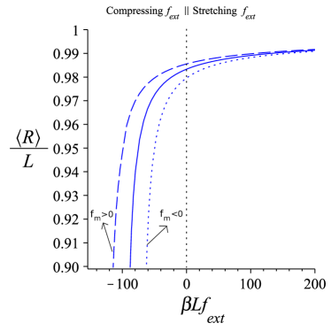
Figure 2: Extension of the filament, Rdelimited-⟨⟩𝑅\langle R\rangle, as a function of the external force fextsubscript𝑓𝑒𝑥𝑡f_{ext} which can be compressive or extensile; full line: no motor attached; dashed line βLfm=+50𝛽𝐿subscript𝑓𝑚50\beta Lf_{m}=+50; dotted line: βLfm=50𝛽𝐿subscript𝑓𝑚50\beta Lf_{m}=-50; (parameters: L=1𝐿1L=1, lp=10subscript𝑙𝑝10l_{p}=10, L/Lm=2𝐿subscript𝐿𝑚2L/L_{m}=2; hinged-hinged filament)
Refer to caption
Refer to caption
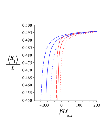
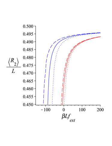
Figure 3: Extension of the two separate parts of the filament, R1delimited-⟨⟩subscript𝑅1\langle R_{1}\rangle and R2delimited-⟨⟩subscript𝑅2\langle R_{2}\rangle, as a function of the external force, fextsubscript𝑓𝑒𝑥𝑡f_{ext}, for several values of the motor force; red lines: clamped-free filament; blue lines: hinged-hinged filament. (full lines: no motor attached; dashed lines βLfm=+50𝛽𝐿subscript𝑓𝑚50\beta Lf_{m}=+50; dotted lines: βLfm=50𝛽𝐿subscript𝑓𝑚50\beta Lf_{m}=-50; parameters as in Fig.2)
Refer to caption
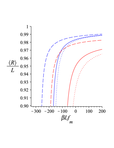
Figure 4: Extension of the filament, Rdelimited-⟨⟩𝑅\langle R\rangle, as a function of the motor force fmsubscript𝑓𝑚f_{m} for several values of the external force; red lines: clamped-free filament, blue lines: hinged-hinged filament. (full lines: no motor attached; dashed lines βLfext=+50𝛽𝐿subscript𝑓𝑒𝑥𝑡50\beta Lf_{ext}=+50; dotted lines: βLfext=10𝛽𝐿subscript𝑓𝑒𝑥𝑡10\beta Lf_{ext}=-10; parameters as in Fig.2)
Refer to caption
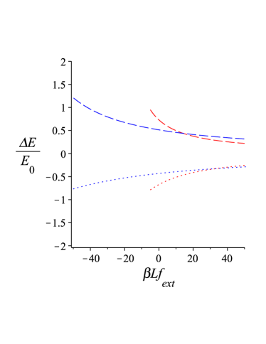
Figure 5: Change in the differential stiffness relative to the case without a spring as a function of the external force; red lines: clamped-free filament, blue lines: hinged-hinged filamen; (dashed lines βLfm=+50𝛽𝐿subscript𝑓𝑚50\beta Lf_{m}=+50; dotted lines: βLfm=50𝛽𝐿subscript𝑓𝑚50\beta Lf_{m}=-50; parameters as in Fig.2).

The explicit analytic solution for the Green function is given in the appendix. As a result we obtain analytic, albeit lengthy expressions for the force extension R=R(fext)delimited-⟨⟩𝑅delimited-⟨⟩𝑅subscript𝑓𝑒𝑥𝑡\langle R\rangle=\langle R\rangle(f_{ext}). To better understand these results, we plot the force-extension relations for hinged-hinged boundary conditions in Fig. 2. The effect of the motor force is more pronounced in the compressional regime, fext<0subscript𝑓𝑒𝑥𝑡0f_{ext}<0, because the filament is softer in response to compressions as compared to extensions, fext>0subscript𝑓𝑒𝑥𝑡0f_{ext}>0. The motor force can partially compensate the compression of the fiber by the external force, if its sign is opposite, i.e. it is pulling on the left part of the segment. Obviously, the left segment is then extended as compared to the case without motor (see Fig.3, upper part), but also the right segment is extended (see Fig.3, lower part), even though the tension in the right part does not depend on fmsubscript𝑓𝑚f_{m}. The reason for this extension is the stronger alignment of the left end of the right part of the filament by the motor. The overall effect of a positive motor force is to substantially stiffen the filament in the compressional regime. The effects of course increase with increasing motor force. If the motor force is compressional the extension of the filament is correspondingly reduced as compared to the case without motor force.

In Fig. 4, we show the dependence of the filaments extension on the motor force, fmsubscript𝑓𝑚f_{m}, for several values of external pulling force, fextsubscript𝑓𝑒𝑥𝑡f_{ext}. If no external force is applied R=R(fm)delimited-⟨⟩𝑅delimited-⟨⟩𝑅subscript𝑓𝑚\langle R\rangle=\langle R\rangle(f_{m}) looks qualitatively similar to R=R(fext)delimited-⟨⟩𝑅delimited-⟨⟩𝑅subscript𝑓𝑒𝑥𝑡\langle R\rangle=\langle R\rangle(f_{ext}). The filament is most sensitive to the external pulling force in the range where the motor tends to compress the filament.

The effects of the motor are seen best in the differential tensile stiffness of the filament, which can be computed from the force-extension relation according to

E1=Rfextsuperscript𝐸1delimited-⟨⟩𝑅subscript𝑓𝑒𝑥𝑡E^{-1}=\frac{\partial\langle R\rangle}{\partial f_{ext}} (18)

In Fig. 5 we show the relative change in the differential stiffness of the filament caused by the spring. There is significant enhancement in stiffness when the spring force is extensile (dashed line), because the effective tension of the filament is increased. The stiffness is weakened for a compressive motor force (full lines). In both cases do we observe stronger effects in the regime where the external force is compressive, implying that a filament under compression is strongly sensitive to a motor which is either pushing or pulling.

IV.1 Limit of small motor force fmsubscript𝑓𝑚f_{m}

It is instructive to consider the limit of small motor force fmmin{fext,κL2}much-less-thansubscript𝑓𝑚subscript𝑓𝑒𝑥𝑡𝜅superscript𝐿2f_{m}\ll\min\{f_{ext},\frac{\kappa}{L^{2}}\}. For the clamped-free case, we find

RRfm=0=fmk(fext).delimited-⟨⟩𝑅subscriptdelimited-⟨⟩𝑅subscript𝑓𝑚0subscript𝑓𝑚𝑘subscript𝑓𝑒𝑥𝑡\left\langle R\right\rangle-\left\langle R\right\rangle_{f_{m}=0}=\frac{f_{m}}{k(f_{ext})}. (19)

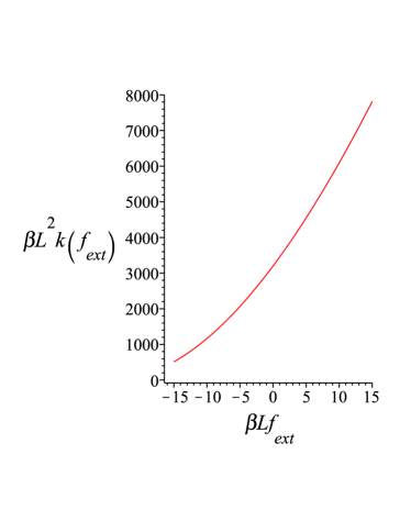
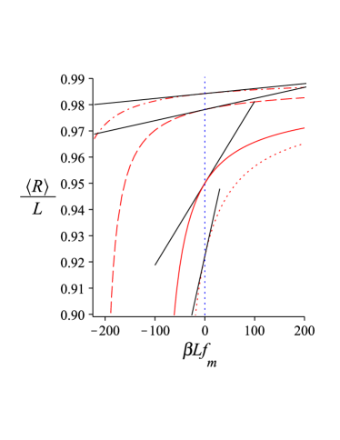
In this limit, the motor-filament system can be represented as a linear elastic element with an effective force constant k𝑘k that depends on the external pulling force and the point of attachment of the motor. The explicit expression for the force constant is given in the Appendix, and a similar expression can be calculated for the hinged-hinged case. In Fig. 6, we show the force constant k𝑘k of the motor as a function of the external force fextsubscript𝑓𝑒𝑥𝑡f_{ext}. The force constant decreases as we compress the filament and it increases as we increase the stretching force. This change of the motor force constant k𝑘k is an essential feature of the elasticity of the semiflexible filament which is missing in studies using linear elasticity for the filament. In Fig. 7, we compare the exact force-extension relation to the linearised one. As can be seen in the figure, the linear approximation works better for higher values of the external force fextsubscript𝑓𝑒𝑥𝑡f_{ext}.

In the limit of large external forces, fextmax{fm,κLm2}much-greater-thansubscript𝑓𝑒𝑥𝑡subscript𝑓𝑚𝜅superscriptsubscript𝐿𝑚2f_{ext}\gg\max\{f_{m},\frac{\kappa}{{L_{m}}^{2}}\}, and large filament length, min{L,Lm}fext/(kBT)much-greater-than𝑚𝑖𝑛𝐿subscript𝐿𝑚subscript𝑓𝑒𝑥𝑡subscript𝑘𝐵𝑇min\{L,L_{m}\}\gg f_{ext}/(k_{B}T), Eq. 19 reduces to the following relation, irrespective of boundary conditions:

RL=112kBTκfext+Lm4LkBTfmκfext32.delimited-⟨⟩𝑅𝐿112subscript𝑘𝐵𝑇𝜅subscript𝑓𝑒𝑥𝑡subscript𝐿𝑚4𝐿subscript𝑘𝐵𝑇subscript𝑓𝑚𝜅superscriptsubscript𝑓𝑒𝑥𝑡32\frac{\left\langle R\right\rangle}{L}=1-\frac{1}{2}\frac{k_{B}T}{\sqrt{\kappa f_{ext}}}+\frac{L_{m}}{4L}\frac{k_{B}Tf_{m}}{\sqrt{\kappa}{f_{ext}}^{\frac{3}{2}}}. (20)

Notice that this equation holds in the thermodynamic limit and it is scale invariant: if we multiply all lengths (Rdelimited-⟨⟩𝑅\left\langle R\right\rangle, Lmsubscript𝐿𝑚L_{m}, L𝐿L) by the same factor, it does not change. The effect of the motor force is subdominant, as it scales with 1/fext3/2similar-toabsent1superscriptsubscript𝑓𝑒𝑥𝑡32\sim 1/f_{ext}^{3/2} compared to 1/fextsimilar-toabsent1subscript𝑓𝑒𝑥𝑡\sim 1/\sqrt{f_{ext}} for the Marko-Siggia case, but it is noteworthy that it persists in the thermodynamic limit and is not just a finite-size effect.

In the limit of small external forces, fextκ/L2much-less-thansubscript𝑓𝑒𝑥𝑡𝜅superscript𝐿2f_{ext}\ll\kappa/L^{2}, we obtain a linear response to both the motor and the external force, which in the case of clamped-free boundary conditions reads:

RcfL=1L2lp+2Lm3LLm46L3lpf~m+L6lpf~ext,subscriptdelimited-⟨⟩𝑅𝑐𝑓𝐿1𝐿2subscript𝑙𝑝2superscriptsubscript𝐿𝑚3𝐿superscriptsubscript𝐿𝑚46superscript𝐿3subscript𝑙𝑝subscript~𝑓𝑚𝐿6subscript𝑙𝑝subscript~𝑓𝑒𝑥𝑡\frac{\left\langle R\right\rangle_{cf}}{L}=1-\frac{L}{2l_{p}}+\frac{2L_{m}^{3}L-L_{m}^{4}}{6L^{3}l_{p}}\tilde{f}_{m}+\frac{L}{6l_{p}}\tilde{f}_{ext}\;, (21)
Refer to caption
Figure 6: Effective stiffness, k(fext)𝑘subscript𝑓𝑒𝑥𝑡k(f_{ext}), of the filament with respect to the motor force as a function of external force fextsubscript𝑓𝑒𝑥𝑡f_{ext}. The range of the external force is chosen in a way that the filament is well approximated as weakly bending (RL>0.9𝑅𝐿0.9\frac{R}{L}>0.9); parameters as in Fig.2).
Refer to caption
Figure 7: Comparison of the complete solution for the end to end distance R/Ldelimited-⟨⟩𝑅𝐿\langle R\rangle/L and the one linearized around fm=0subscript𝑓𝑚0f_{m}=0; full lines: βLfext=0𝛽𝐿subscript𝑓𝑒𝑥𝑡0\beta Lf_{ext}=0; dashed lines βLfext=50𝛽𝐿subscript𝑓𝑒𝑥𝑡50\beta Lf_{ext}=50; dashed-dotted lines: βLfext=100𝛽𝐿subscript𝑓𝑒𝑥𝑡100\beta Lf_{ext}=100; dotted line: βLfext=10𝛽𝐿subscript𝑓𝑒𝑥𝑡10\beta Lf_{ext}=-10 (parameters as in Fig.2).

IV.2 Limit of large motor force fmsubscript𝑓𝑚f_{m}

In the limit of large motor force, fmmax{fext,κLm2}much-greater-thansubscript𝑓𝑚subscript𝑓𝑒𝑥𝑡𝜅superscriptsubscript𝐿𝑚2f_{m}\gg\max\{f_{ext},\frac{\kappa}{{L_{m}}^{2}}\}, we expect the left part of the filament to display the asymptotic (Marko-Siggia) force extension for large fmsubscript𝑓𝑚f_{m} and indeed it does:

R1cf=LmLm2lpκfmsubscriptdelimited-⟨⟩subscript𝑅1𝑐𝑓subscript𝐿𝑚subscript𝐿𝑚2subscript𝑙𝑝𝜅subscript𝑓𝑚\left\langle R_{1}\right\rangle_{cf}=L_{m}-\frac{L_{m}}{2l_{p}}\sqrt{\frac{\kappa}{f_{m}}} (22)

However the extension of the right part of the filament is not just given by the expression for a wormlike chain under tension fextsubscript𝑓𝑒𝑥𝑡f_{ext} but shows a correction of 𝒪(1fm)𝒪1subscript𝑓𝑚{\cal O}(\frac{1}{\sqrt{f_{m}}})

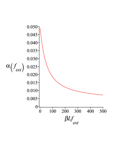
R2cf=R2WLCα(fext)κfm.subscriptdelimited-⟨⟩subscript𝑅2𝑐𝑓subscriptdelimited-⟨⟩subscript𝑅2𝑊𝐿𝐶𝛼subscript𝑓𝑒𝑥𝑡𝜅subscript𝑓𝑚\left\langle R_{2}\right\rangle_{cf}=\left\langle R_{2}\right\rangle_{WLC}-\alpha(f_{ext})\sqrt{\frac{\kappa}{f_{m}}}. (23)

The strength of the effect depends on the external pulling force (see Fig. 8) and is strongest for weak pulling force. Explicit forms of R2WLCsubscriptdelimited-⟨⟩subscript𝑅2𝑊𝐿𝐶\left\langle R_{2}\right\rangle_{WLC} and α(fext)𝛼subscript𝑓𝑒𝑥𝑡\alpha(f_{ext}) are given in the Appendix.

Refer to caption
Figure 8: Coefficient of the asymptotic expansion, α(fext)𝛼subscript𝑓𝑒𝑥𝑡\alpha(f_{ext}), as function of external force fextsubscript𝑓𝑒𝑥𝑡f_{ext}; (parameters as in Fig.2).

In the limit of small external force, fextκ/L2fmmuch-less-thansubscript𝑓𝑒𝑥𝑡𝜅superscript𝐿2much-less-thansubscript𝑓𝑚f_{ext}\ll\kappa/L^{2}\ll f_{m} and κ/Lm2fmmuch-less-than𝜅superscriptsubscript𝐿𝑚2subscript𝑓𝑚\kappa/L_{m}^{2}\ll f_{m}, we obtain a linear force-extension relation:

RcfLsubscriptdelimited-⟨⟩𝑅𝑐𝑓𝐿\displaystyle\frac{\left\langle R\right\rangle_{cf}}{L} =1L2lp+Lm(6L3Lm)6lpL+(LLm)46L3lpf~extabsent1𝐿2subscript𝑙𝑝subscript𝐿𝑚6𝐿3subscript𝐿𝑚6subscript𝑙𝑝𝐿superscript𝐿subscript𝐿𝑚46superscript𝐿3subscript𝑙𝑝subscript~𝑓𝑒𝑥𝑡\displaystyle=1-\frac{L}{2l_{p}}+\frac{L_{m}(6L-3L_{m})}{6l_{p}L}+\frac{(L-L_{m})^{4}}{6L^{3}l_{p}}\tilde{f}_{ext} (24)
(6L3Lm)Lm6lpL1f~m12.6𝐿3subscript𝐿𝑚subscript𝐿𝑚6subscript𝑙𝑝𝐿1superscriptsubscript~𝑓𝑚12\displaystyle-\frac{(6L-3L_{m})L_{m}}{6l_{p}L}\frac{1}{\tilde{f}_{m}^{\frac{1}{2}}}\;.

IV.3 Limit of large force fextsubscript𝑓𝑒𝑥𝑡f_{ext} and fm=fext+ϵsubscript𝑓𝑚subscript𝑓𝑒𝑥𝑡italic-ϵf_{m}=-f_{ext}+\epsilon

Next, we consider the limit of a large external pulling force, which is almost compensated by the motor in the left part of the filament. In other words, we put fm=fext+ϵsubscript𝑓𝑚subscript𝑓𝑒𝑥𝑡italic-ϵf_{m}=-f_{ext}+\epsilon and consider the case with fextκLm2much-greater-thansubscript𝑓𝑒𝑥𝑡𝜅superscriptsubscript𝐿𝑚2f_{ext}\gg\frac{\kappa}{{L_{m}}^{2}} and ϵκL2much-less-thanitalic-ϵ𝜅superscript𝐿2\epsilon\ll\frac{\kappa}{{L}^{2}}. In this limit, the right part of the filament is asymptotically extended

R2cf=LLm(LLm2lp)(κfext)1/2.subscriptdelimited-⟨⟩subscript𝑅2𝑐𝑓𝐿subscript𝐿𝑚𝐿subscript𝐿𝑚2subscript𝑙𝑝superscript𝜅subscript𝑓𝑒𝑥𝑡12\left\langle R_{2}\right\rangle_{cf}=L-L_{m}-(\frac{L-L_{m}}{2l_{p}})(\frac{\kappa}{f_{ext}})^{1/2}. (25)

The total extension in this limit is given by

RcfL=Lm26lp(L6lp)(3LLm)f~ext12+(Lm490lpL2)ϵ~.subscriptdelimited-⟨⟩𝑅𝑐𝑓𝐿superscriptsubscript𝐿𝑚26subscript𝑙𝑝𝐿6subscript𝑙𝑝3𝐿subscript𝐿𝑚superscriptsubscript~𝑓𝑒𝑥𝑡12superscriptsubscript𝐿𝑚490subscript𝑙𝑝superscript𝐿2~italic-ϵ\left\langle R\right\rangle_{cf}-L=\frac{L_{m}^{2}}{6l_{p}}-(\frac{L}{6l_{p}})\frac{(3L-L_{m})}{\tilde{f}_{ext}^{\frac{1}{2}}}+(\frac{L_{m}^{4}}{90l_{p}L^{2}})\tilde{\epsilon}. (26)

The first term accounts for the reduction in length due to thermal fluctuations in the left part only and hence Lm2proportional-toabsentsuperscriptsubscript𝐿𝑚2\propto L_{m}^{2}. The tension in the left part is just ϵ1much-less-thanitalic-ϵ1\epsilon\ll 1 which accounts for the last term. However the pulling force fextsubscript𝑓𝑒𝑥𝑡f_{ext} affects the orientation of the tangent at Lmsubscript𝐿𝑚L_{m} and hence also the extension of the left part of the filament so the dominant term for strong pulling force is not just determined by the right part of the filament.

V relation to single-motor experiments

Our results can be tested experimentally using optical tweezers. Beads attached to the two ends of the biomolecule which acts as track (e.g., F-actin) are trapped with optical tweezers. The motor (e.g., myosin-V) is attached with one end to a fixed bead and with the other end to the filament. Since the two end beads are free to rotate, this arrangement corresponds to the case of hinged-hinged boundary conditions. This experimental set-up has already been used in many single-molecule mechanical transducers Veigel_Schmidt_NR2011 . The ”three-bead” technique was pioneered by Finer et al. Finer_1994 . The main idea is to measure the variance of the end-beads’ position which is related to the stiffness of the actomyosin cross-bridge complex within linear elasticity Veigel_Molloy_2001 ; Veigel_1998 . Conformational changes in the motor induce changes in the effective stiffness of the bridge which is measured experimentally. In our model, the conformational change in myosin changes the motor force fmsubscript𝑓𝑚f_{m}. This can be due to a change in the position of attachment of the myosin head on the actin filament, Lmsubscript𝐿𝑚L_{m}, or a change in the effective spring constant, kmsubscript𝑘𝑚k_{m}, or both.

Our results have been obtained in the fixed force ensemble, where the tension on the filament is determined sharply and this results in a fluctuating extension, whose average we have calculated. The positions of the motor bead, which determines X0subscript𝑋0X_{0} in our model, and of the left filament end are held fixed. This can be done by using a very stiff optical trap. As shown by Gerland et al. in Gerland_Bundschuh_Hwa , a polymer held between two optical traps is represented by the mixed ensemble, where both the tension and the extension fluctuate. This mixed ensemble interpolates between the fixed extension ensemble (corresponding to the limit of very stiff traps) and fixed force ensemble (corresponding to the limit of very soft traps). Therefore, our general results for hinged-hinged boundary conditions can be tested with a set up involving a very soft optical trap for the right end of the filament. We should point out, that the force-extension relation given by Eq. 20 holds in the thermodynamic limit and as such is ensemble independent (fixed force or fixed extension). In addition, the linear response results are ensemble independent.

In real systems, the spring will act not only in the longitudinal direction but also in the transverse direction. The effect of a transverse spring of zero rest length in the force-extension relation of a weakly bending wormlike chain has been calculated in PB_SU_AZ_NJP . For a spring of finite rest length which is almost parallel to the longitudinal direction of the filament, the transverse effect is of higher order and can be neglected. For a spring of zero rest length but with fm0subscript𝑓𝑚0f_{m}\neq 0, we can simply add the following contribution to the right-hand side of Eq. 20:

ΔRL=kmkBT4fext2(1+kmL2fext)1,Δdelimited-⟨⟩𝑅𝐿subscript𝑘𝑚subscript𝑘𝐵𝑇4superscriptsubscript𝑓𝑒𝑥𝑡2superscript1subscript𝑘𝑚𝐿2subscript𝑓𝑒𝑥𝑡1\displaystyle\frac{\Delta\langle R\rangle}{L}=\frac{k_{m}k_{B}T}{4f_{ext}^{2}}\Big{(}1+\frac{k_{m}L}{2f_{ext}}\Big{)}^{-1}, (27)

which holds in the strong stretching limit, fκ/Lm2much-greater-than𝑓𝜅superscriptsubscript𝐿𝑚2f\gg\kappa/L_{m}^{2}. For a soft spring, kmLfextmuch-less-thansubscript𝑘𝑚𝐿subscript𝑓𝑒𝑥𝑡k_{m}L\ll f_{ext}, this contribution falls off as fext2similar-toabsentsuperscriptsubscript𝑓𝑒𝑥𝑡2\sim f_{ext}^{-2}, which is subdominant to the longitudinal contribution which falls off as fext3/2similar-toabsentsuperscriptsubscript𝑓𝑒𝑥𝑡32\sim f_{ext}^{-3/2}.

VI Conclusion-Outlook

We have analysed the force-extension of a wormlike chain whose one end is fixed, while the other end is pulled or pushed by an external force. In addition, the filament is attached to a spring which may represent a cross-link or a motor arrested at its stall force. Irrespective of boundary conditions, the effects of the spring are stronger in the compressive regime as compared to the stretching regime. Depending on the relative sign of the pulling force and the spring force, the latter can substantially stiffen or weaken the filament. When the motor force is small, its effects can be represented by an effective spring constant which strongly depends on the prestress of the fiber, i.e. the external force. When the motor force is large, it gives rise to the same 1/fext1subscript𝑓𝑒𝑥𝑡1/\sqrt{f_{ext}} dependence which is well known from the work of Marko and Siggia Marko_Siggia .

The dependence of the force extension curve of the filament on motor force allows to deduce the latter from measurements of the force-extension relation. In fact the so-called three bead geometry has already been used to determine the stiffness of the actomyosin cross-bridge Veigel_1998 .

An interesting direction for future work is the study of two or more parallel-aligned filaments with non-local spring-like cross-linkers in the direction of alignment. The case of local cross-links has been investigated in Alice1 ; Alice2 ; PB_SU_AZ_NJP . A simplified model of two filaments with a non-local spring has been studied in Liverpool_Marchetti_EPL2009 .

VII Acknowledgement

We thank the DFG for financial support through SFB 937, project A1.

VIII Appendix

A.1. Filament with hinged-hinged boundary conditions at the two tips

The force is a piecewise constant function with two pieces. As result of this fact, the Green function is a piecewise function with six pieces:

G(s,s)={G1(s,s)0<s<sLm<LG1+(s,s)0<s<sLm<LG2(s,s)0<Lms<s<LG2+(s,s)0<Lms<s<LG3(s,s)0<s<Lm<s<LG3+(s,s)0<s<Lm<s<L𝐺𝑠superscript𝑠casessuperscriptsubscript𝐺1𝑠superscript𝑠0𝑠superscript𝑠subscript𝐿𝑚𝐿superscriptsubscript𝐺1𝑠superscript𝑠0superscript𝑠𝑠subscript𝐿𝑚𝐿otherwiseotherwisesuperscriptsubscript𝐺2𝑠superscript𝑠0subscript𝐿𝑚𝑠superscript𝑠𝐿superscriptsubscript𝐺2𝑠superscript𝑠0subscript𝐿𝑚superscript𝑠𝑠𝐿otherwiseotherwisesuperscriptsubscript𝐺3𝑠superscript𝑠0𝑠subscript𝐿𝑚superscript𝑠𝐿superscriptsubscript𝐺3𝑠superscript𝑠0superscript𝑠subscript𝐿𝑚𝑠𝐿G(s,s^{\prime})=\begin{cases}G_{1}^{-}(s,s^{\prime})&0<s<s^{\prime}\leq L_{m}<L\\ G_{1}^{+}(s,s^{\prime})&0<s^{\prime}<s\leq L_{m}<L\\ \\ G_{2}^{-}(s,s^{\prime})&0<L_{m}\leq s<s^{\prime}<L\\ G_{2}^{+}(s,s^{\prime})&0<L_{m}\leq s^{\prime}<s<L\\ \\ G_{3}^{-}(s,s^{\prime})&0<s<L_{m}<s^{\prime}<L\\ G_{3}^{+}(s,s^{\prime})&0<s^{\prime}<L_{m}<s<L\\ \end{cases} (28)

The assumption that the derivative of the tangent vector is zero at the end tips (hinged-hinged condition) leads to the vanishing of the derivative of the Green function. Considering the boundary conditions, the solution for the aforementioned equation must have the following form:

Ghh(s,s)={G1(s,s)=N11(s)cosh(sσ1)G1+(s,s)=N12(s)(cosh(sσ1)+A1sinh(sσ1))G2(s,s)=N21(s)(cosh(sσ2)+A2sinh(sσ2))G2+(s,s)=N22(s)cosh((Ls)σ2)G3(s,s)=N31(s)cosh(sσ1)G3+(s,s)=N32(s)cosh((Ls)σ2),subscript𝐺𝑠superscript𝑠casessuperscriptsubscript𝐺1𝑠superscript𝑠subscript𝑁11superscript𝑠𝑠subscript𝜎1otherwisesuperscriptsubscript𝐺1𝑠superscript𝑠subscript𝑁12superscript𝑠𝑠subscript𝜎1subscript𝐴1𝑠subscript𝜎1otherwiseotherwiseotherwisesuperscriptsubscript𝐺2𝑠superscript𝑠subscript𝑁21superscript𝑠𝑠subscript𝜎2subscript𝐴2𝑠subscript𝜎2otherwisesuperscriptsubscript𝐺2𝑠superscript𝑠subscript𝑁22superscript𝑠𝐿𝑠subscript𝜎2otherwiseotherwiseotherwisesuperscriptsubscript𝐺3𝑠superscript𝑠subscript𝑁31superscript𝑠𝑠subscript𝜎1otherwisesuperscriptsubscript𝐺3𝑠superscript𝑠subscript𝑁32superscript𝑠𝐿𝑠subscript𝜎2otherwiseG_{hh}(s,s^{\prime})=\begin{cases}G_{1}^{-}(s,s^{\prime})=N_{11}(s^{\prime})\cosh(s\sigma_{1})\\ G_{1}^{+}(s,s^{\prime})=N_{12}(s^{\prime})(\cosh(s\sigma_{1})+A_{1}\sinh(s\sigma_{1}))\\ \\ G_{2}^{-}(s,s^{\prime})=N_{21}(s^{\prime})(\cosh(s\sigma_{2})+A_{2}\sinh(s\sigma_{2}))\\ G_{2}^{+}(s,s^{\prime})=N_{22}(s^{\prime})\cosh((L-s)\sigma_{2})\\ \\ G_{3}^{-}(s,s^{\prime})=N_{31}(s^{\prime})\cosh(s\sigma_{1})\\ G_{3}^{+}(s,s^{\prime})=N_{32}(s^{\prime})\cosh((L-s)\sigma_{2})\;,\\ \end{cases} (29)

where σ(s)=f(s)κ={σ1=f1κ0<s<Lmσ2=f2κLm<s<L𝜎𝑠𝑓𝑠𝜅casessubscript𝜎1subscript𝑓1𝜅0𝑠subscript𝐿𝑚otherwiseotherwisesubscript𝜎2subscript𝑓2𝜅subscript𝐿𝑚𝑠𝐿\sigma(s)=\sqrt{\frac{f(s)}{\kappa}}=\begin{cases}\sigma_{1}=\sqrt{\frac{f_{1}}{\kappa}}&0<s<L_{m}\\ \\ \sigma_{2}=\sqrt{\frac{f_{2}}{\kappa}}&L_{m}<s<L\end{cases} and Lmsubscript𝐿𝑚L_{m} is the position of molecular motor in terms of the contour length. Moreover, constants appearing in eq. 29 are obtained from the following conditions:

{G1+(s,s)ss=sG1(s,s)ss=s=1βκ(1)G1(s,s)=G1+(s,s)(2)G2+(s,s)ss=sG2(s,s)ss=s=1βκ(3)G2(s,s)=G2+(s,s)(4)G3(Lm,s)=G2(Lm,s)(5)G3+(Lm,s)=G1+(Lm,s)(6)G3(s,s)ss=Lm=G2(s,s)ss=Lm(7)G3+(s,s)ss=Lm=G1+(s,s)ss=Lm(8).casesevaluated-atsuperscriptsubscript𝐺1𝑠superscript𝑠𝑠𝑠superscript𝑠evaluated-atsuperscriptsubscript𝐺1𝑠superscript𝑠𝑠𝑠superscript𝑠1𝛽𝜅1superscriptsubscript𝐺1superscript𝑠superscript𝑠superscriptsubscript𝐺1superscript𝑠superscript𝑠2otherwiseotherwiseevaluated-atsuperscriptsubscript𝐺2𝑠superscript𝑠𝑠𝑠superscript𝑠evaluated-atsuperscriptsubscript𝐺2𝑠superscript𝑠𝑠𝑠superscript𝑠1𝛽𝜅3superscriptsubscript𝐺2superscript𝑠superscript𝑠superscriptsubscript𝐺2superscript𝑠superscript𝑠4otherwiseotherwisesuperscriptsubscript𝐺3subscript𝐿𝑚superscript𝑠superscriptsubscript𝐺2subscript𝐿𝑚superscript𝑠5superscriptsubscript𝐺3subscript𝐿𝑚superscript𝑠superscriptsubscript𝐺1subscript𝐿𝑚superscript𝑠6otherwiseotherwiseevaluated-atsuperscriptsubscript𝐺3𝑠superscript𝑠𝑠𝑠subscript𝐿𝑚evaluated-atsuperscriptsubscript𝐺2𝑠superscript𝑠𝑠𝑠subscript𝐿𝑚7evaluated-atsuperscriptsubscript𝐺3𝑠superscript𝑠𝑠𝑠subscript𝐿𝑚evaluated-atsuperscriptsubscript𝐺1𝑠superscript𝑠𝑠𝑠subscript𝐿𝑚8\begin{cases}\frac{\partial G_{1}^{+}(s,s^{\prime})}{\partial s}\mid_{s=s^{\prime}}-\frac{\partial G_{1}^{-}(s,s^{\prime})}{\partial s}\mid_{s=s^{\prime}}=-\frac{1}{\beta\kappa}&(1)\\ G_{1}^{-}(s^{\prime},s^{\prime})=G_{1}^{+}(s^{\prime},s^{\prime})&(2)\\ \\ \frac{\partial G_{2}^{+}(s,s^{\prime})}{\partial s}\mid_{s=s^{\prime}}-\frac{\partial G_{2}^{-}(s,s^{\prime})}{\partial s}\mid_{s=s^{\prime}}=-\frac{1}{\beta\kappa}&(3)\\ G_{2}^{-}(s^{\prime},s^{\prime})=G_{2}^{+}(s^{\prime},s^{\prime})&(4)\\ \\ G_{3}^{-}(L_{m},s^{\prime})=G_{2}^{-}(L_{m},s^{\prime})&(5)\\ G_{3}^{+}(L_{m},s^{\prime})=G_{1}^{+}(L_{m},s^{\prime})&(6)\\ \\ \frac{\partial G_{3}^{-}(s,s^{\prime})}{\partial s}\mid_{s=L_{m}}=\frac{\partial G_{2}^{-}(s,s^{\prime})}{\partial s}\mid_{s=L_{m}}&(7)\\ \frac{\partial G_{3}^{+}(s,s^{\prime})}{\partial s}\mid_{s=L_{m}}=\frac{\partial G_{1}^{+}(s,s^{\prime})}{\partial s}\mid_{s=L_{m}}&(8)\;.\end{cases} (30)

These conditions coming in Eq. 30, except number (7) and number (8), gives:

{N11(s)=cosh(σ1s)+A1sinh(σ1s)σ1lpA1N12(s)=cosh(σ1s)σ1lpA1N21(s)=cosh(σ2(Ls))σ2lp(sinh(σ2L)+A2cosh(σ2L))N22(s)=cosh(σ2s)+A2sinh(σ2s)σ2lp(sinh(σ2L)+A2cosh(σ2L))N31(s)=cosh(σ2(Ls)(cosh(σ2Lm)+A2sinh(σ2Lm)))σ2lpcosh(σ1Lm)(sinh(σ2L)+A2cosh(σ2L))N32(s)=cosh(σ1s)(cosh(σ1Lm)+A1sinh(σ1Lm))σ1lpA1cosh(σ2(LLm)),casessubscript𝑁11superscript𝑠subscript𝜎1superscript𝑠subscript𝐴1subscript𝜎1superscript𝑠subscript𝜎1subscript𝑙𝑝subscript𝐴1otherwiseotherwiseotherwisesubscript𝑁12superscript𝑠subscript𝜎1superscript𝑠subscript𝜎1subscript𝑙𝑝subscript𝐴1otherwiseotherwiseotherwisesubscript𝑁21superscript𝑠subscript𝜎2𝐿superscript𝑠subscript𝜎2subscript𝑙𝑝subscript𝜎2𝐿subscript𝐴2subscript𝜎2𝐿otherwiseotherwiseotherwisesubscript𝑁22superscript𝑠subscript𝜎2superscript𝑠subscript𝐴2subscript𝜎2superscript𝑠subscript𝜎2subscript𝑙𝑝subscript𝜎2𝐿subscript𝐴2subscript𝜎2𝐿otherwiseotherwiseotherwisesubscript𝑁31superscript𝑠subscript𝜎2𝐿superscript𝑠subscript𝜎2subscript𝐿𝑚subscript𝐴2subscript𝜎2subscript𝐿𝑚subscript𝜎2subscript𝑙𝑝subscript𝜎1subscript𝐿𝑚subscript𝜎2𝐿subscript𝐴2subscript𝜎2𝐿otherwiseotherwiseotherwisesubscript𝑁32superscript𝑠subscript𝜎1superscript𝑠subscript𝜎1subscript𝐿𝑚subscript𝐴1subscript𝜎1subscript𝐿𝑚subscript𝜎1subscript𝑙𝑝subscript𝐴1subscript𝜎2𝐿subscript𝐿𝑚otherwise\begin{cases}N_{11}(s^{\prime})=-\frac{\cosh(\sigma_{1}s^{\prime})+A_{1}\sinh(\sigma_{1}s^{\prime})}{\sigma_{1}l_{p}A_{1}}\\ \\ N_{12}(s^{\prime})=-\frac{\cosh(\sigma_{1}s^{\prime})}{\sigma_{1}l_{p}A_{1}}\\ \\ N_{21}(s^{\prime})=\frac{\cosh(\sigma_{2}(L-s^{\prime}))}{\sigma_{2}l_{p}(\sinh(\sigma_{2}L)+A_{2}\cosh(\sigma_{2}L))}\\ \\ N_{22}(s^{\prime})=\frac{\cosh(\sigma_{2}s^{\prime})+A_{2}\sinh(\sigma_{2}s^{\prime})}{\sigma_{2}l_{p}(\sinh(\sigma_{2}L)+A_{2}\cosh(\sigma_{2}L))}\\ \\ N_{31}(s^{\prime})=\frac{\cosh(\sigma_{2}(L-s^{\prime})(\cosh(\sigma_{2}L_{m})+A_{2}\sinh(\sigma_{2}L_{m})))}{\sigma_{2}l_{p}\cosh(\sigma_{1}L_{m})(\sinh(\sigma_{2}L)+A_{2}\cosh(\sigma_{2}L))}\\ \\ N_{32}(s^{\prime})=-\frac{\cosh(\sigma_{1}s^{\prime})(\cosh(\sigma_{1}L_{m})+A_{1}\sinh(\sigma_{1}L_{m}))}{\sigma_{1}l_{p}A_{1}\cosh(\sigma_{2}(L-L_{m}))}\;,\end{cases} (31)

The conditions number (7) and number (8) of eq. 30 give:

{A1=σ2sinh(σ2(LLm))cosh(σ1Lm)+σ1sinh(σ1Lm)cosh(σ2(LLm))σ2sinh(σ2(LLm))sinh(σ1Lm)+σ1cosh(σ1Lm)cosh(σ2(LLm))A2=σ1sinh(σ1Lm)cosh(σ2Lm)σ2sinh(σ2Lm)cosh(σ1Lm)σ1sinh(σ1Lm)sinh(σ2Lm)σ2cosh(σ2Lm)cosh(σ1Lm)casessubscript𝐴1subscript𝜎2subscript𝜎2𝐿subscript𝐿𝑚subscript𝜎1subscript𝐿𝑚subscript𝜎1subscript𝜎1subscript𝐿𝑚subscript𝜎2𝐿subscript𝐿𝑚subscript𝜎2subscript𝜎2𝐿subscript𝐿𝑚subscript𝜎1subscript𝐿𝑚subscript𝜎1subscript𝜎1subscript𝐿𝑚subscript𝜎2𝐿subscript𝐿𝑚otherwiseotherwiseotherwisesubscript𝐴2subscript𝜎1subscript𝜎1subscript𝐿𝑚subscript𝜎2subscript𝐿𝑚subscript𝜎2subscript𝜎2subscript𝐿𝑚subscript𝜎1subscript𝐿𝑚subscript𝜎1subscript𝜎1subscript𝐿𝑚subscript𝜎2subscript𝐿𝑚subscript𝜎2subscript𝜎2subscript𝐿𝑚subscript𝜎1subscript𝐿𝑚otherwise\begin{cases}A_{1}=-\frac{\sigma_{2}\sinh(\sigma_{2}(L-L_{m}))\cosh(\sigma_{1}L_{m})+\sigma_{1}\sinh(\sigma_{1}L_{m})\cosh(\sigma_{2}(L-L_{m}))}{\sigma_{2}\sinh(\sigma_{2}(L-L_{m}))\sinh(\sigma_{1}L_{m})+\sigma_{1}\cosh(\sigma_{1}L_{m})\cosh(\sigma_{2}(L-L_{m}))}\\ \\ A_{2}=-\frac{\sigma_{1}\sinh(\sigma_{1}L_{m})\cosh(\sigma_{2}L_{m})-\sigma_{2}\sinh(\sigma_{2}L_{m})\cosh(\sigma_{1}L_{m})}{\sigma_{1}\sinh(\sigma_{1}L_{m})\sinh(\sigma_{2}L_{m})-\sigma_{2}\cosh(\sigma_{2}L_{m})\cosh(\sigma_{1}L_{m})}\par\end{cases} (32)

Concerning the boundary condition, the correlation function of the transverse components of tangent vector is written as follows:

ai(s)ai(s)hh=limJi0δ2ln(Z(Ji))δJi(s)δJi(s),subscriptdelimited-⟨⟩subscript𝑎𝑖𝑠subscript𝑎𝑖superscript𝑠subscriptsubscript𝐽𝑖0superscript𝛿2𝑍subscript𝐽𝑖𝛿subscript𝐽𝑖𝑠𝛿subscript𝐽𝑖superscript𝑠\left<a_{i}(s)a_{i}(s^{\prime})\right>_{hh}=\lim_{J_{i}\rightarrow 0}\frac{\delta^{2}\ln\left(Z(J_{i})\right)}{\delta J_{i}(s)\delta J_{i}(s^{\prime})}\;, (33)

where Z(Ji)=D{ai(s)}δ(0L𝑑sai(s))exp(βHWBA+0L𝑑sJi(s)ai(s))𝑍subscript𝐽𝑖𝐷subscript𝑎𝑖𝑠𝛿superscriptsubscript0𝐿differential-d𝑠subscript𝑎𝑖𝑠𝛽subscript𝐻𝑊𝐵𝐴superscriptsubscript0𝐿differential-d𝑠subscript𝐽𝑖𝑠subscript𝑎𝑖𝑠Z(J_{i})=\int D\left\{a_{i}(s)\right\}\delta(\int_{0}^{L}dsa_{i}(s))\exp(-\beta H_{WBA}+\int_{0}^{L}dsJ_{i}(s)a_{i}(s)) is the generating functional with source term Ji(s)subscript𝐽𝑖𝑠J_{i}(s) and β=1kBT𝛽1subscript𝑘𝐵𝑇\beta=\frac{1}{k_{B}T}. The correlation function of the transverse components of the tangent vector is obtained by the following expression hori2007stretching ; peskin1995introduction :

ai(s)ai(s)=Ghh(s,s)oLGhh(s,s1)𝑑s1oLGhh(s,s2)𝑑s20L0LGhh(s1,s2)𝑑s1𝑑s2delimited-⟨⟩subscript𝑎𝑖𝑠subscript𝑎𝑖superscript𝑠subscript𝐺𝑠superscript𝑠superscriptsubscript𝑜𝐿subscript𝐺𝑠subscript𝑠1differential-dsubscript𝑠1superscriptsubscript𝑜𝐿subscript𝐺superscript𝑠subscript𝑠2differential-dsubscript𝑠2superscriptsubscript0𝐿superscriptsubscript0𝐿subscript𝐺subscript𝑠1subscript𝑠2differential-dsubscript𝑠1differential-dsubscript𝑠2\displaystyle\left<a_{i}(s)a_{i}(s^{\prime})\right>=G_{hh}(s,s^{\prime})-\frac{\int_{o}^{L}G_{hh}(s,s_{1})ds_{1}\int_{o}^{L}G_{hh}(s^{\prime},s_{2})ds_{2}}{\int_{0}^{L}\int_{0}^{L}G_{hh}(s_{1},s_{2})ds_{1}ds_{2}} (34)

which implies

ai2(s)=Ghh(s,s)(oLGhh(s,s1)𝑑s1)20L0LGhh(s1,s2)𝑑s1𝑑s2delimited-⟨⟩superscriptsubscript𝑎𝑖2𝑠subscript𝐺𝑠𝑠superscriptsuperscriptsubscript𝑜𝐿subscript𝐺𝑠subscript𝑠1differential-dsubscript𝑠12superscriptsubscript0𝐿superscriptsubscript0𝐿subscript𝐺subscript𝑠1subscript𝑠2differential-dsubscript𝑠1differential-dsubscript𝑠2\displaystyle\left<{a_{i}}^{2}(s)\right>=G_{hh}(s,s)-\frac{\left(\int_{o}^{L}G_{hh}(s,s_{1})ds_{1}\right)^{2}}{\int_{0}^{L}\int_{0}^{L}G_{hh}(s_{1},s_{2})ds_{1}ds_{2}} (35)

A.2. Filament with clamped-free boundary conditions at the two end tips

In the clamped-free case, we enforce the transverse components of the tangent vector of the filament at s=0𝑠0s=0 and their derivitive at s=L𝑠𝐿s=L to be zero. Similar to Appendix 1, we obtain the following expression for the Green function:

Gcf(s,s)={G1(s,s)sinh(σ1s)(B1cosh(σ1s)+sinh(σ1s))lpσ1B1G1+(s,s)(B1cosh(σ1s)+sinh(σ1s))sinh(σ1s)lpσ1B1G2(s,s)cosh(σ2(Ls))(B2cosh(σ2s)+sinh(σ2s))lpσ2B2sinh(σ2L)+lpσ2cosh(σ2L)G2+(s,s)cosh(σ2s)(B2cosh(σ2s)+sinh(σ2s))lpσ2B2sinh(σ2L)+lpσ2cosh(σ2L)G3(s,s)sinh(σ1s)cosh(σ2(Ls))(B2cosh(σ2Lm)+sinh(σ2Lm))lpσ2sinh(σ1Lm)(B2sinh(σ2L)+cosh(σ2L))G3+(s,s)cosh(σ2(Ls))sinh(σ1s)(B1cosh(σ1Lm)+sinh(σ1Lm))lpσ1B1cosh(σ2(LLm))subscript𝐺𝑐𝑓𝑠superscript𝑠casessuperscriptsubscript𝐺1𝑠superscript𝑠subscript𝜎1𝑠subscript𝐵1subscript𝜎1superscript𝑠subscript𝜎1superscript𝑠subscript𝑙𝑝subscript𝜎1subscript𝐵1otherwiseotherwiseotherwisesuperscriptsubscript𝐺1𝑠superscript𝑠subscript𝐵1subscript𝜎1𝑠subscript𝜎1𝑠subscript𝜎1superscript𝑠subscript𝑙𝑝subscript𝜎1subscript𝐵1otherwiseotherwiseotherwiseotherwiseotherwisesuperscriptsubscript𝐺2𝑠superscript𝑠subscript𝜎2𝐿superscript𝑠subscript𝐵2subscript𝜎2𝑠subscript𝜎2𝑠subscript𝑙𝑝subscript𝜎2subscript𝐵2subscript𝜎2𝐿subscript𝑙𝑝subscript𝜎2subscript𝜎2𝐿otherwiseotherwiseotherwisesuperscriptsubscript𝐺2𝑠superscript𝑠subscript𝜎2𝑠subscript𝐵2subscript𝜎2superscript𝑠subscript𝜎2superscript𝑠subscript𝑙𝑝subscript𝜎2subscript𝐵2subscript𝜎2𝐿subscript𝑙𝑝subscript𝜎2subscript𝜎2𝐿otherwiseotherwiseotherwiseotherwiseotherwisesuperscriptsubscript𝐺3𝑠superscript𝑠subscript𝜎1𝑠subscript𝜎2𝐿superscript𝑠subscript𝐵2subscript𝜎2subscript𝐿𝑚subscript𝜎2subscript𝐿𝑚subscript𝑙𝑝subscript𝜎2subscript𝜎1subscript𝐿𝑚subscript𝐵2subscript𝜎2𝐿subscript𝜎2𝐿otherwiseotherwiseotherwisesuperscriptsubscript𝐺3𝑠superscript𝑠subscript𝜎2𝐿𝑠subscript𝜎1superscript𝑠subscript𝐵1subscript𝜎1subscript𝐿𝑚subscript𝜎1subscript𝐿𝑚subscript𝑙𝑝subscript𝜎1subscript𝐵1subscript𝜎2𝐿subscript𝐿𝑚otherwiseG_{cf}(s,s^{\prime})=\begin{cases}G_{1}^{-}(s,s^{\prime})\equiv\frac{\sinh(\sigma_{1}s)(B_{1}\cosh(\sigma_{1}s^{\prime})+\sinh(\sigma_{1}s^{\prime}))}{l_{p}\sigma_{1}B_{1}}\\ \\ G_{1}^{+}(s,s^{\prime})\equiv\frac{(B_{1}\cosh(\sigma_{1}s)+\sinh(\sigma_{1}s))\sinh(\sigma_{1}s^{\prime})}{l_{p}\sigma_{1}B_{1}}\\ \\ \\ G_{2}^{-}(s,s^{\prime})\equiv\frac{\cosh(\sigma_{2}(L-s^{\prime}))(B_{2}\cosh(\sigma_{2}s)+\sinh(\sigma_{2}s))}{l_{p}\sigma_{2}B_{2}\sinh(\sigma_{2}L)+l_{p}\sigma_{2}\cosh(\sigma_{2}L)}\\ \\ G_{2}^{+}(s,s^{\prime})\equiv\frac{\cosh(\sigma_{2}s)(B_{2}\cosh(\sigma_{2}s^{\prime})+\sinh(\sigma_{2}s^{\prime}))}{l_{p}\sigma_{2}B_{2}\sinh(\sigma_{2}L)+l_{p}\sigma_{2}\cosh(\sigma_{2}L)}\\ \\ \\ G_{3}^{-}(s,s^{\prime})\equiv\frac{\sinh(\sigma_{1}s)\cosh(\sigma_{2}(L-s^{\prime}))(B_{2}\cosh(\sigma_{2}L_{m})+\sinh(\sigma_{2}L_{m}))}{l_{p}\sigma_{2}\sinh(\sigma_{1}L_{m})(B_{2}\sinh(\sigma_{2}L)+\cosh(\sigma_{2}L))}\\ \\ G_{3}^{+}(s,s^{\prime})\equiv\frac{\cosh(\sigma_{2}(L-s))\sinh(\sigma_{1}s^{\prime})(B_{1}\cosh(\sigma_{1}L_{m})+\sinh(\sigma_{1}L_{m}))}{l_{p}\sigma_{1}B_{1}\cosh(\sigma_{2}(L-L_{m}))}\\ \end{cases} (36)

where:

{B1=σ2sinh(σ2(LLm))sinh(σ1Lm)+σ1cosh(σ2(LLm))cosh(σ1Lm)σ2sinh(σ2(LLm))cosh(σ1Lm)+σ1cosh(σ2(LLm))sinh(σ1Lm)B2=σ1cosh(σ1Lm)sinh(σ2Lm)σ2sinh(σ1Lm)cosh(σ2Lm)σ2sinh(σ1Lm)sinh(σ2Lm)σ1cosh(σ1Lm)cosh(σ2Lm)casessubscript𝐵1subscript𝜎2subscript𝜎2𝐿subscript𝐿𝑚subscript𝜎1subscript𝐿𝑚subscript𝜎1subscript𝜎2𝐿subscript𝐿𝑚subscript𝜎1subscript𝐿𝑚subscript𝜎2subscript𝜎2𝐿subscript𝐿𝑚subscript𝜎1subscript𝐿𝑚subscript𝜎1subscript𝜎2𝐿subscript𝐿𝑚subscript𝜎1subscript𝐿𝑚otherwiseotherwiseotherwisesubscript𝐵2subscript𝜎1subscript𝜎1subscript𝐿𝑚subscript𝜎2subscript𝐿𝑚subscript𝜎2subscript𝜎1subscript𝐿𝑚subscript𝜎2subscript𝐿𝑚subscript𝜎2subscript𝜎1subscript𝐿𝑚subscript𝜎2subscript𝐿𝑚subscript𝜎1subscript𝜎1subscript𝐿𝑚subscript𝜎2subscript𝐿𝑚otherwise\begin{cases}B_{1}=-\frac{\sigma_{2}\sinh(\sigma_{2}(L-L_{m}))\sinh(\sigma_{1}L_{m})+\sigma_{1}\cosh(\sigma_{2}(L-L_{m}))\cosh(\sigma_{1}L_{m})}{\sigma_{2}\sinh(\sigma_{2}(L-L_{m}))\cosh(\sigma_{1}L_{m})+\sigma_{1}\cosh(\sigma_{2}(L-L_{m}))\sinh(\sigma_{1}L_{m})}\\ \\ B_{2}=\frac{\sigma_{1}\cosh(\sigma_{1}L_{m})\sinh(\sigma_{2}L_{m})-\sigma_{2}\sinh(\sigma_{1}L_{m})\cosh(\sigma_{2}L_{m})}{\sigma_{2}\sinh(\sigma_{1}L_{m})\sinh(\sigma_{2}L_{m})-\sigma_{1}\cosh(\sigma_{1}L_{m})\cosh(\sigma_{2}L_{m})}\par\end{cases} (37)

The correlation function hori2007stretching ; peskin1995introduction is obtained as follows:

ai(s)ai(s)cf=Gcf(s,s)subscriptdelimited-⟨⟩subscript𝑎𝑖𝑠subscript𝑎𝑖superscript𝑠𝑐𝑓subscript𝐺𝑐𝑓𝑠superscript𝑠\left<a_{i}(s)a_{i}(s^{\prime})\right>_{cf}=G_{cf}(s,s^{\prime}) (38)

which implies

ai2(s)cf=Gcf(s,s)subscriptdelimited-⟨⟩subscriptsuperscript𝑎2𝑖𝑠𝑐𝑓subscript𝐺𝑐𝑓𝑠𝑠\left<a^{2}_{i}(s)\right>_{cf}=G_{cf}(s,s) (39)

A.3  Linear end to end distance in terms of fmsubscript𝑓𝑚f_{m}

The end to end distance of the whole filament when it is in the clamped-free condition can be written as follows:

Rcf=LL2tanh(f~ext12)2lpf~ext+(1k(fext))fmsubscriptdelimited-⟨⟩𝑅𝑐𝑓𝐿superscript𝐿2superscriptsubscript~𝑓𝑒𝑥𝑡122subscript𝑙𝑝subscript~𝑓𝑒𝑥𝑡1𝑘subscript𝑓𝑒𝑥𝑡subscript𝑓𝑚\left\langle R\right\rangle_{cf}=L-\frac{L^{2}\tanh(\tilde{f}_{ext}^{\frac{1}{2}})}{2l_{p}\tilde{f}_{ext}}+\left(\frac{1}{k(f_{ext})}\right){f_{m}} (40)

The effective linear motor force constant k is:

1k1𝑘\displaystyle\frac{1}{k} =14(lpκ(fextκ)52(e4Lfextκ+2e2Lfextκ+1))absent14subscript𝑙𝑝𝜅superscriptsubscript𝑓𝑒𝑥𝑡𝜅52superscript𝑒4𝐿subscript𝑓𝑒𝑥𝑡𝜅2superscript𝑒2𝐿subscript𝑓𝑒𝑥𝑡𝜅1\displaystyle=-\frac{1}{4\left(l_{p}\kappa(\frac{f_{ext}}{\kappa})^{\frac{5}{2}}(e^{4L\sqrt{\frac{f_{ext}}{\kappa}}}+2e^{2L\sqrt{\frac{f_{ext}}{\kappa}}}+1)\right)} (41)
×\displaystyle\times [Ae4Lfextκ+Be2(2LLm)fextκ+Ce2Lfextκ++De2(L+Lm)fextκ+Ee2(LLm)fextκ+Fe2Lmfextκ+G],\displaystyle\left[Ae^{4L\sqrt{\frac{f_{ext}}{\kappa}}}+Be^{2(2L-L_{m})\sqrt{\frac{f_{ext}}{\kappa}}}+Ce^{2L\sqrt{\frac{f_{ext}}{\kappa}}}++De^{2(L+L_{m})\sqrt{\frac{f_{ext}}{\kappa}}}+Ee^{2(L-L_{m})\sqrt{\frac{f_{ext}}{\kappa}}}+Fe^{2L_{m}\sqrt{\frac{f_{ext}}{\kappa}}}+G\right]\;,

where A=fextLmκ+fextκ,B=(fextLmκ+fextκ),C=(4fextLLmκ+2)fextκ,D=(fextκfextLmκ+fextLκ),E=fextκfextLmκ+fextLκ,F=fextLmκfextκ,G=fextLmκ+fextκformulae-sequence𝐴subscript𝑓𝑒𝑥𝑡subscript𝐿𝑚𝜅subscript𝑓𝑒𝑥𝑡𝜅formulae-sequence𝐵subscript𝑓𝑒𝑥𝑡subscript𝐿𝑚𝜅subscript𝑓𝑒𝑥𝑡𝜅formulae-sequence𝐶4subscript𝑓𝑒𝑥𝑡𝐿subscript𝐿𝑚𝜅2subscript𝑓𝑒𝑥𝑡𝜅formulae-sequence𝐷subscript𝑓𝑒𝑥𝑡𝜅subscript𝑓𝑒𝑥𝑡subscript𝐿𝑚𝜅subscript𝑓𝑒𝑥𝑡𝐿𝜅formulae-sequence𝐸subscript𝑓𝑒𝑥𝑡𝜅subscript𝑓𝑒𝑥𝑡subscript𝐿𝑚𝜅subscript𝑓𝑒𝑥𝑡𝐿𝜅formulae-sequence𝐹subscript𝑓𝑒𝑥𝑡subscript𝐿𝑚𝜅subscript𝑓𝑒𝑥𝑡𝜅𝐺subscript𝑓𝑒𝑥𝑡subscript𝐿𝑚𝜅subscript𝑓𝑒𝑥𝑡𝜅A=-\frac{f_{ext}L_{m}}{\kappa}+\sqrt{\frac{f_{ext}}{\kappa}},B=-\left(\frac{f_{ext}L_{m}}{\kappa}+\sqrt{\frac{f_{ext}}{\kappa}}\right),C=\left(\frac{4f_{ext}LL_{m}}{\kappa}+2\right)\sqrt{\frac{f_{ext}}{\kappa}},D=-\left(\sqrt{\frac{f_{ext}}{\kappa}}-\frac{f_{ext}L_{m}}{\kappa}+\frac{f_{ext}L}{\kappa}\right),E=-\sqrt{\frac{f_{ext}}{\kappa}}-\frac{f_{ext}L_{m}}{\kappa}+\frac{f_{ext}L}{\kappa},F=\frac{f_{ext}L_{m}}{\kappa}-\sqrt{\frac{f_{ext}}{\kappa}},G=\frac{f_{ext}L_{m}}{\kappa}+\sqrt{\frac{f_{ext}}{\kappa}}

VIII.1 A.4 Limit of large motor force fmsubscript𝑓𝑚f_{m}

In the limit of large motor forces fmMax{fext,κL2}much-greater-thansubscript𝑓𝑚𝑀𝑎𝑥subscript𝑓𝑒𝑥𝑡𝜅superscript𝐿2f_{m}\gg Max\{f_{ext},\frac{\kappa}{{L}^{2}}\}, we have the following expression for the end to end distance of the first piece of the filament:

R1cf=LmLm2lpκfmsubscriptdelimited-⟨⟩subscript𝑅1𝑐𝑓subscript𝐿𝑚subscript𝐿𝑚2subscript𝑙𝑝𝜅subscript𝑓𝑚\left\langle R_{1}\right\rangle_{cf}=L_{m}-\frac{L_{m}}{2l_{p}}\sqrt{\frac{\kappa}{f_{m}}} (42)

and the end to end distance of the second piece of the filament:

R2cfsubscriptdelimited-⟨⟩subscript𝑅2𝑐𝑓\displaystyle\left\langle R_{2}\right\rangle_{cf} =(LLm)(LLm)2lptanh((LLm)fextκ)fextκabsent𝐿subscript𝐿𝑚𝐿subscript𝐿𝑚2subscript𝑙𝑝𝐿subscript𝐿𝑚subscript𝑓𝑒𝑥𝑡𝜅subscript𝑓𝑒𝑥𝑡𝜅\displaystyle=\left(L-L_{m}\right)-\frac{\left(L-L_{m}\right)}{2l_{p}}\frac{\tanh\left(\left(L-L_{m}\right)\sqrt{\frac{f_{ext}}{\kappa}}\right)}{\sqrt{\frac{f_{ext}}{\kappa}}}
α(fext)κfm,𝛼subscript𝑓𝑒𝑥𝑡𝜅subscript𝑓𝑚\displaystyle-\alpha(f_{ext})\sqrt{\frac{\kappa}{f_{m}}}\;,

where

α(fext)𝛼subscript𝑓𝑒𝑥𝑡\displaystyle\alpha(f_{ext}) =e4Lfextκe4Lmfextκ2lpfextκ(e2Lfextκ+e2Lmfextκ)2absentsuperscript𝑒4𝐿subscript𝑓𝑒𝑥𝑡𝜅superscript𝑒4subscript𝐿𝑚subscript𝑓𝑒𝑥𝑡𝜅2subscript𝑙𝑝subscript𝑓𝑒𝑥𝑡𝜅superscriptsuperscript𝑒2𝐿subscript𝑓𝑒𝑥𝑡𝜅superscript𝑒2subscript𝐿𝑚subscript𝑓𝑒𝑥𝑡𝜅2\displaystyle=\frac{e^{4L\sqrt{\frac{f_{ext}}{\kappa}}}-e^{4L_{m}\sqrt{\frac{f_{ext}}{\kappa}}}}{2l_{p}\sqrt{\frac{f_{ext}}{\kappa}}\left(e^{2L\sqrt{\frac{f_{ext}}{\kappa}}}+e^{2L_{m}\sqrt{\frac{f_{ext}}{\kappa}}}\right)^{2}}
+2(LLm)e2(L+Lm)fextκlp(e2Lfextκ+e2Lmfextκ)22𝐿subscript𝐿𝑚superscript𝑒2𝐿subscript𝐿𝑚subscript𝑓𝑒𝑥𝑡𝜅subscript𝑙𝑝superscriptsuperscript𝑒2𝐿subscript𝑓𝑒𝑥𝑡𝜅superscript𝑒2subscript𝐿𝑚subscript𝑓𝑒𝑥𝑡𝜅2\displaystyle+\frac{2(L-L_{m})e^{2(L+L_{m})\sqrt{\frac{f_{ext}}{\kappa}}}}{l_{p}\left(e^{2L\sqrt{\frac{f_{ext}}{\kappa}}}+e^{2L_{m}\sqrt{\frac{f_{ext}}{\kappa}}}\right)^{2}}

References

  • [1] Adam J. Engler, Shamik Sen, H. Lee Sweeney, and Dennis E. Discher. Matrix elasticity directs stem cell lineage specification. Cell, 126(4):677 – 689, 2006.
  • [2] Darci T. Butcher, Tamara Alliston, and Valerie M. Weaver. A tense situation: forcing tumour progression. Nat Rev Cancer, 9(2):108–122, 02 Nat Rev Cancer.
  • [3] Tadanori Mammoto and Donald E. Ingber. Mechanical control of tissue and organ development. Development, 137(9):1407–1420, 2010.
  • [4] AR Bausch and K Kroy. A bottom-up approach to cell mechanics. Nature physics, 2(4):231–238, 2006.
  • [5] Robyn H. Pritchard, Yan Yan Shery Huang, and Eugene M. Terentjev. Mechanics of biological networks: from the cell cytoskeleton to connective tissue. Soft Matter, 10:1864–1884, 2014.
  • [6] C. P. Broedersz and F. C. MacKintosh. Modeling semiflexible polymer networks. Rev. Mod. Phys., 86:995–1036, Jul 2014.
  • [7] Oliver Lieleg, Mireille M. A. E. Claessens, and Andreas R. Bausch. Structure and dynamics of cross-linked actin networks. Soft Matter, 6:218–225, 2010.
  • [8] Steven J. Winder and Kathryn R. Ayscough. Actin-binding proteins. Journal of Cell Science, 118(4):651–654, 2005.
  • [9] Eckhard Mandelkow and Eva-Maria Mandelkow. Microtubules and microtubule-associated proteins. Current Opinion in Cell Biology, 7(1):72 – 81, 1995.
  • [10] Claudia Veigel and Christoph F. Schmidt. Moving into the cell: single-molecule studies of molecular motors in complex environments. Nat Rev Mol Cell Biol, 12(3):163–176, 03 2011.
  • [11] Erika LF Holzbaur and Yale E Goldman. Coordination of molecular motors: From in vitro assays to intracellular dynamics. Current opinion in cell biology, 22(1):4–13, 02 2010.
  • [12] A. F. Huxley. Muscle structure and theories of contraction. PROGRESS IN BIOPHYSICS AND BIOPHYSICAL CHEMISTRY, 7:255–318, 1957.
  • [13] Thomas Guérin, Jacques Prost, Pascal Martin, and Jean-François Joanny. Coordination and collective properties of molecular motors: theory. Current Opinion in Cell Biology, 22(1):14–20, 2 2010.
  • [14] John F. Marko and Eric D. Siggia. Stretching dna. Macromolecules, 28(26):8759–8770, 1995.
  • [15] Azam Gholami, Jan Wilhelm, and Erwin Frey. Entropic forces generated by grafted semiflexible polymers. Phys. Rev. E, 74:041803, Oct 2006.
  • [16] Yuko Hori, Ashok Prasad, and Jané Kondev. Stretching short biopolymers by fields and forces. Physical Review E, 75(4):041904, 2007.
  • [17] Michael E Peskin and Daniel V Schroeder. An introduction to quantum field theory. Westview, 1995.
  • [18] Jeffrey T. Finer, Robert M. Simmons, and James A. Spudich. Single myosin molecule mechanics: piconewton forces and nanometre steps. Nature, 368(6467):113–119, 03 1994.
  • [19] Claudia Veigel, Fei Wang, Marc L. Bartoo, James R. Sellers, and Justin E. Molloy. The gated gait of the processive molecular motor, myosin v. Nat Cell Biol, 4(1):59–65, 01 2002.
  • [20] Claudia Veigel, Marc L. Bartoo, David C. S. White, John C. Sparrow, and Justin E. Molloy. The stiffness of rabbit skeletal actomyosin cross-bridges determined with an optical tweezers transducer. Biophysical Journal, 75:1424, 1998.
  • [21] Ulrich Gerland, Ralf Bundschuh, and Terence Hwa. Mechanically probing the folding pathway of single rna molecules. Biophysical Journal, 84(5):2831–2840, 05 2003.
  • [22] Panayotis Benetatos, Stephan Ulrich, and Annette Zippelius. Force–extension relation of cross-linked anisotropic polymer networks. New Journal of Physics, 14(11):115011, 2012.
  • [23] Alice von der Heydt, Daniel Wilkin, Panayotis Benetatos, and Annette Zippelius. Elasticity of cross-linked semiflexible biopolymers under tension. Phys. Rev. E, 88:032701, Sep 2013.
  • [24] Panayotis Benetatos, Alice von der Heydt, and Annette Zippelius. Tension-induced binding of semiflexible biopolymers. New Journal of Physics, 16(11):113037, 2014.
  • [25] T. B. Liverpool, M. C. Marchetti, J.-F. Joanny, and J. Prost. Mechanical response of active gels. EPL (Europhysics Letters), 85(1):18007, 2009.