Initial-data contribution to the error budget of gravitational waves from neutron-star binaries

Abstract

As numerical calculations of inspiralling neutron-star binaries reach values of accuracy that are comparable with those of binary black holes, a fine budgeting of the various sources of error becomes increasingly important. Among such sources, the initial data is normally not accounted for, the rationale being that the error on the initial spacelike hypersurface is always far smaller than the one gained during the evolution. We here consider critically this assumption and perform a comparative analysis of the gravitational waveforms relative to essentially the same physical binary configuration when computed with two different initial-data codes, and then evolved with the same evolution code. More specifically, we consider the evolution of irrotational neutron-star binaries computed either with the pseudo-spectral code lorene, or with the newly developed finite-difference code cocal; both sets of initial data are subsequently evolved with the high-order evolution code WhiskyTHC. In this way we find that despite the initial data shows global (local) differences that are $\lesssim 0.02\%\ (1\%)$, the gravitational-wave phase at the merger time differs by $\sim 0.5$ radians after $\sim 3$ orbits, a surprisingly large value. Our results highlight the highly nonlinear impact that errors in the initial data can have on the subsequent evolution and the importance of using exactly the same initial data when comparative studies are done.

I Introduction

With the first direct detection of gravitational waves from a merging system of black holes Abbott et al. (2016), the long awaited gravitational-wave astronomy has finally become a reality in which a series of advanced interferometers such as LIGO, GEO, Virgo, KAGRA, ET Abramovici et al. (1992); Accadia et al. (2011); Kuroda and LCGT Collaboration (2010); Aso et al. (2013); Punturo et al. (2010) is eagerly operating to unveil that part of the universe that can be observed in terms of gravitational radiation. Neutron star binary systems are prime actors of this universe and have received enormous attention over the last ten years.

In addition, neutron-star binaries are leading candidates for the engine of short gamma ray bursts Narayan et al. (1992); Eichler et al. (1989); Rezzolla et al. (2011); Bartos et al. (2013); Berger (2014), and possible sites for the production of the heaviest elements in the universe Lattimer and Schramm (1974); Li and Paczynski (1998); Tanvir et al. (2013); Berger et al. (2013); Tanaka and Hotokezaka (2013); Rosswog et al. (2014); Sekiguchi et al. (2015); Radice et al. (2016). Starting from the first successful simulations of binary neutron-star mergers Shibata and Uryū (2000) and the first complete description of this process from the inspiral down to the formation of an accreting black-hole–torus system Baiotti et al. (2008), considerable progress has been done, so that it is now possible to consider rather realistic scenarios involving nuclear-physics equations of state Sekiguchi et al. (2011a); Takami et al. (2015), neutrino cooling Sekiguchi et al. (2011b); Galeazzi et al. (2013); Sekiguchi et al. (2015); Radice et al. (2016) and magnetohydrodynamics Anderson et al. (2008); Liu et al. (2008); Giacomazzo et al. (2009); Kiuchi et al. (2014); Dionysopoulou et al. (2015).

Obviously, any simulation of neutron-star binaries needs initial data to get started and this is carefully crafted through standalone codes like cocal Uryū et al. (2012); Tsokaros et al. (2015), lorene Lorene Website , kadath Grandclement (2010), scrid Tichy (2009, 2012), or through the elliptic solvers of the evolution codes like spec SpEC Website , Princeton’s East et al. (2012), or bam Brügmann et al. (2008). Although the first initial data for neutron-star binaries has been computed for corotating systems Baumgarte et al. (1998), the large majority of the simulations performed to date has used irrotational configurations, since neutron star viscosity is believed to be too small to tidally lock the two stars prior to merger Kochanek (1992); Bildsten and Cutler (1992). At the same time, the most advanced efforts over the last couple of years have been concentrated on approaches to reduce the eccentricity of the orbits or to produce binary systems with arbitrary neutron star spins Kyutoku et al. (2014); Moldenhauer et al. (2014); Bernuzzi et al. (2014); Tichy (2012); Kastaun et al. (2013); Tsatsin and Marronetti (2013); Tsokaros et al. (2015); Dietrich et al. (2015); Tacik et al. (2015).

In the past, the cocal code has been used to compute quasi-equilibrium sequences for binary black holes Uryū and Tsokaros (2012); Uryū et al. (2012); Tsokaros and Uryū (2012), and a pointwise comparison was made with the spectral code kadath, both for the gravitational fields, as well as for global quantities like the ADM mass and angular momentum, finding excellent agreement. More recently, the cocal code has been used to compute quasi-equilibrium sequences neutron-star binaries that are irrotational or spinning, with spins aligned with the orbital angular momentum Tsokaros et al. (2015); also in this case, the comparison with the lorene code for irrotational sequences has shown excellent agreement. Overall, both sets of studies show that when considering close binaries of compact objects, be it black holes or neutron stars, the use of cocal has led to agreements in the global quantities to less than $0.03\%$, while for the individual metric components the differences were less than $1\%$.

In this work we focus on neutron-star binaries and perform a close comparison with another spectral code, lorene, not only for the data on the initial slice, but also for its subsequent evolution. More specifically, given irrotational binaries of neutron stars produced by either lorene or cocal, we consider the same physical initial data in terms of gravitational mass, rest mass, orbital frequency, and evolve both sets of initial data with the high-order code WhiskyTHC Radice et al. (2014a, b, 2015). The evolutions are performed at a number of resolutions, the highest of which have spacings of $\delta x=0.1\,M_{\odot}\simeq 150\,{\rm m}$ and represent a major computational cost, which has been reported before for one binary only in Radice et al. (2015), where it is referred to as “very high”. Across all simulations, we have monitored in detail the violations of the constraint equations and we have performed a gravitational-wave analysis with respect to the phase of the $\ell=m=2$ mode of the Weyl scalar $\Psi_{4}$. Although the initial data between cocal and lorene shows global (local) differences that are $\lesssim 0.02\%\ (1\%)$, or that the waveforms have only very small differences, and that even the convergence properties of the gravitational-wave signal are almost identical for the two sets of initial data, we find that the Richardson-extrapolated phases differ by an order of magnitude, i.e., of about one radian, at the merger time, after $\sim 3$ orbits. These results highlight therefore the highly nonlinear impact that errors in the initial data can have on the subsequent evolution, so that extra care needs to be employed when computing waveforms of neutron-star binaries spanning tens of orbits. More importantly, because this is the first time that evolutions from different initial-data solvers is presented, our results issue an important warning signal about the importance of using exactly the same initial data when comparative studies of neutron star binary evolutions, such as the ones carried out in Baiotti et al. (2010); Read et al. (2013), are performed.

The plan of the paper is as follows. In Section II we provide a review of the quasiequilibrium equations and present the cocal driver to the cactus Cactus Website infrastructure, while in Section III we describe the techniques developed to import the initial data produced by cocal in an evolution code, performing a global and local close comparison of an irrotational binary as computed with lorene and with cocal. Section IV is instead dedicated to the detailed comparison of the evolution of the two sets of initial data for the various configurations considered and to the presentation of the corresponding convergence properties. Finally, our conclusions are presented in V. As complementary material, we present in Appendix A a short study for corotating initial data produced by cocal and lorene, again at $45\,{\rm km}$, mostly as a benchmark of future arbitrary spinning binaries.

Hereafter, spacetime indices running from $0$ to $3$ will be indicated with Greek letters, while spatial indices running from $1$ to $3$ with Latin letters. The metric has signature $(-,+,+,+,)$, and we use a set of geometric units in which $G=c=M_{\odot}=1$, unless stated otherwise (we recall that in these units $1\,M_{\odot}=4.92674\,{\rm\mu s}=1.477\,{\rm km}$).

II Review of the quasiequilibrium equations

In this Section we only state the basic definitions and equations that are solved while we refer to Tsokaros et al. (2015) and references within for more details. The spacetime metric in a $3+1$ decomposition is written as

$$ds^{2}=-\alpha^{2}dt^{2}+\gamma_{ij}(dx^{i}+\beta^{i}dt)(dx^{j}+\beta^{j}dt)\,,$$ (1)

where $\alpha,\ \beta^{i},\ \gamma_{ij}$ are, respectively, the lapse function, the shift vector, and the three-metric on some spacelike slice $\Sigma_{t}$, which is taken to be conformally flat

$$\gamma_{ij}=\psi^{4}\delta_{ij}\,.$$ (2)

Here we use the Cartesian components of the shift. The extrinsic curvature is defined as $K_{\alpha\beta}:=-\frac{1}{2}\mathcal{L}_{\bm{n}}\gamma_{\alpha\beta}$, where $\mathcal{L}_{\bm{n}}$ is the Lie derivative along the (timelike) unit vector normal $\bm{n}$ to $\Sigma_{t}$. The assumption of stationarity, $\partial_{t}\gamma_{\alpha\beta}=0$, yields $K_{ij}=\frac{1}{2\alpha}\mathcal{L}_{\bm{\beta}}\gamma_{ij}$, while assuming maximal slicing the conformally rescaled trace-free part of the extrinsic curvature becomes

$$\tilde{A}^{ij}=\frac{1}{2\alpha}\left(\partial^{i}\beta^{j}+\partial^{j}\beta^{i}-\frac{2}{3}\delta^{ij}\partial_{k}\beta^{k}\right)=\frac{1}{2\alpha}(\widetilde{\mathbb{L}}\beta)^{ij}\,.$$ (3)

Note that $\tilde{A}_{i}^{\ j}=A_{i}^{\ j}$. The last term in Eq. (3) is the longitudinal operator and the tilde symbol denotes the fact that it is related to the conformally flat geometry.

With the help of Eq. (3), the constraint equations and the spatial trace of the time derivative of the extrinsic curvature (assuming $\partial_{t}K=0$), result in five elliptic equations for the conformal factor $\psi$, the shift $\beta^{i}$, and the lapse function $\alpha$

$$\nabla^{2}\psi=-\frac{\psi^{5}}{32\alpha^{2}}(\widetilde{\mathbb{L}}\beta)^{ab}(\widetilde{\mathbb{L}}\beta)^{ij}\delta_{ia}\delta_{jb}-2\pi E\psi^{5}\,,$$ (4)

$$\nabla^{2}(\alpha\psi)=\frac{7\psi^{5}}{32\alpha}(\widetilde{\mathbb{L}}\beta)^{ab}(\widetilde{\mathbb{L}}\beta)^{ij}\delta_{ia}\delta_{jb}+2\pi\alpha\psi^{5}(E+2S)\,,$$ (5)

$$\nabla^{2}\beta^{i}=-\frac{1}{3}\partial^{i}\partial_{j}\beta^{j}+\partial_{j}\ln\left(\frac{\alpha}{\psi^{6}}\right)(\widetilde{\mathbb{L}}\beta)^{ij}+16\pi\alpha\psi^{4}j^{i}\,,\qquad$$ (6)

where the matter sources are $E:=n_{\alpha}n_{\beta}T^{\alpha\beta}$, $S:=\gamma_{\alpha\beta}T^{\alpha\beta}$, and $j^{i}:=-\gamma^{i}{}_{\alpha}n_{\beta}T^{\alpha\beta}$. The boundary conditions for the equations above are dictated by asymptotic flatness, i.e., $\lim_{r\rightarrow\infty}\psi=1$, $\lim_{r\rightarrow\infty}\alpha=1$, and $\lim_{r\rightarrow\infty}\beta^{i}=0$.

For the stress-energy tensor we assume a perfect fluid with

$$T_{\alpha\beta}=(\epsilon+p)u_{\alpha}u_{\beta}+pg_{\alpha\beta}=\rho hu_{\alpha}u_{\beta}+pg_{\alpha\beta}\,,$$ (7)

where $u^{\alpha}$ is the four-velocity of the fluid and $\rho,\epsilon,h$, and $p$ are, respectively, the rest-mass density, the total energy density, the specific enthalpy, and the pressure as measured in the rest frame of the fluid (see Rezzolla and Zanotti (2013) for details). The specific internal energy $e$ is related to the enthalpy through $h:=({\epsilon+p})/{\rho}=1+e+{p}/{\rho}$. The 4-velocity is decomposed as $u^{\alpha}=u^{t}(t^{\alpha}+v^{\alpha})$ or $u^{\alpha}=u^{t}(k^{\alpha}+V^{\alpha})$ which correspond to an inertial frame or the corotating frame decomposition, respectively. For the fluid variables we assume helical symmetry,

$$\mathcal{L}_{\mathbf{k}}(hu_{\alpha})=\mathcal{L}_{\mathbf{k}}\rho=0\,,$$ (8)

where

$$k^{\mu}:=t^{\mu}+\Omega\phi^{\mu}\,,$$ (9)

is the helical Killing vector, and, without loss of generality,

$$\phi^{i}=(-y,x,0)\,,$$ (10)

is the rotational generator. For corotating binaries, $V^{\alpha}=0$, and the Euler equation results into a first integral

$$\frac{h}{u^{t}}=C,\quad\mbox{with}\quad u^{t}=\frac{1}{\sqrt{\alpha^{2}-\omega_{i}\omega^{i}}}\,.$$ (11)

where $\omega^{i}:=\beta^{i}+\Omega\phi^{i}$ is the corotating shift. For irrotational binaries $hu_{\alpha}=\nabla_{\alpha}\Phi$, $\Phi$ being the fluid velocity potential, and the first integral of the Euler equation is

$$\frac{h}{u^{t}}+V^{j}D_{j}\Phi=C,\quad h=\sqrt{\lambda^{2}/\alpha^{2}-D_{i}\Phi D^{i}\Phi}\,,$$ (12)

with $\lambda:=C+\omega^{i}D_{i}\Phi$. The fluid potential $\Phi$ is determined from conservation of rest mass, $\nabla_{\alpha}(\rho u^{\alpha})=0$, which yields

$$\nabla^{2}\Phi = -\frac{2}{\psi}\partial_{i}\psi\partial^{i}\Phi+\psi^{4}\omega^{i}\partial_{i}(hu^{t})$$ (13)

$$+[\psi^{4}hu^{t}\omega^{i}-\partial^{i}\Phi]\partial_{i}\ln\left(\frac{\alpha\rho}{h}\right)\,,$$

with boundary condition on the star surface

$$\left[\left(\psi^{4}hu^{t}\omega^{i}-\partial^{i}\Phi\right)\partial_{i}\rho\right]_{{\rm surf.}}=0\,.$$ (14)

This condition is derived either from Eq. (13) assuming that the baryon density vanishes on the stellar surface, or by demanding that the fluid velocity is tangent to the stellar surface in the corotating frame $[V^{\mu}\nabla_{\mu}\rho]_{\rm surf.}=0$. Equations (4)–(6) will be solved together with (11) for corotating motion or (12) and (13) for irrotational motion, and the two involving constants $\Omega,\ C$ will be determined in the process. Details about the methods we use in cocal to solve these equations are described in Tsokaros et al. (2015).

Figure 1: Structure of a two-dimensional cross-section of the cocal grids (colored spherical coordinates) overlaid on a Cartesian coordinate system used for the evolution of the initial data. Here we assume that the $z=0$ plane of the evolutionary grid coincides with the corresponding cocal plane. Evolution gridpoints $P(x_{p},y_{p},z_{p})$ inside the sphere of radius $R_{i}$ are interpolated from the coordinate patches COCP-1 or COCP-2 depending whether $x_{p}\leq 0$ or $x_{p}>0$. Points outside that sphere are interpolated from the asymptotic region patch ARCP. Note that the figure is not in scale; in particular, the size of the sphere of radius $R_{i}$ is much larger than the size of the inner boundary $S_{a}$ of ARCP. The outer boundary of ARCP is not shown here and extends to very large values when compared to the compact-object sizes. Typical values are $r_{b}=100$, $d_{s}=2.5$, $d=1.25$, $R_{s}=98.75$, $R_{i}=69.125$, $r_{a}=5.0$. The point where the neutron-star’s surface intersects the positive $x$-axis of the COCP takes values $r_{s}\leq 1$ and is in general different for the two stars.

III Initial data import and comparison

cocal uses finite differences on spherical coordinates to compute the various field variables. Importing the initial data into an evolution code involves interpolating from the cocal grid to the one used by the evolution code, which in most cases is in Cartesian coordinates. In this Section we describe the coc$2$cac driver, which interpolates the cocal grid variables to the Einstein Toolkit Löffler et al. (2012); Einstein Toolkit Website . The full description of the coordinate systems used by cocal can be found in Uryū and Tsokaros (2012) for black hole binaries or Tsokaros et al. (2015) for neutron-star binaries. Here, we review the most salient features that will be necessary for the coc$2$cac driver.

III.1 The coc$2$cac driver

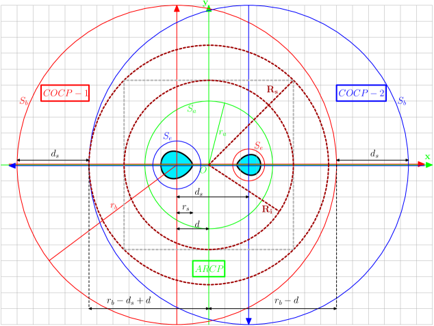
As customary in a $3+1$ decomposition, the spacetime manifold $\mathcal{M}=\mathbb{R}\times\Sigma_{t}$, is foliated by a family of spacelike hypersurface $\Sigma_{t}$, parametrized by $t\in{\mathbb{R}}$. These hypersurfaces may represent data that is stationary (in equilibrium), or quasi-stationary (in quasi-equilibrium) and they are covered by overlapping multiple spherical coordinate patches. In Fig. 1, three such coordinate systems are used to cover the hypersurface. One can think of Fig. 1 as the equatorial plane of a neutron-star binary system. Two spherical coordinate patches are used to cover the area around each neutron star. They are called COCP-1 (from compact object coordinate patch) and COCP-2 and are plotted with red and blue colors, respectively. COCP-1 (COCP-2) include all points inside the outer red (blue) sphere $S_{b}$ of radius $r_{b}$, but outside the red (blue) excised sphere $S_{e}$. Note that these two systems have opposite $(x,y)$ coordinates, but the same $z$ orientation. The reason for introducing the excised sphere $S_{e}$, Tsokaros and Uryū (2007), is to be able to resolve the second compact object with reasonable resources. Without it, the size of the companion neutron star has to be resolved by angular grids, while by using this concept, it is enough to resolve the size of $S_{e}$, which is $\sim d_{s}/2$. This implies that the angle to be resolved is $\sim 2\arcsin 1/2=\pi/3$. As a rule of thumb, the angular resolution of a COCP is determined from the degree of accuracy to resolve the deformation of the neutron stars centered at the patch, and to resolve the size of their excised sphere. The third patch, called the asymptotic-region coordinate patch or ARCP, is denoted by green lines and includes all points outside the sphere $S_{a}$ and infinity, typically a sphere $S_{b}$ not shown here at very large distance from the center of mass $O$.

$r_{a}$:	Radial coordinate where the radial grids start. For
	the COCP patch it is $r_{a}=0$.
$r_{b}$:	Radial coordinate where the radial grids end.
$r_{c}$:	Center of mass point. Excised sphere is located
	at $2r_{c}$ in the COCP patch.
$r_{e}$:	Radius of the excised sphere. Only in the COCP patch.
$r_{s}$:	Radius of the sphere bounding the star’s surface.
	It is $r_{s}\leq 1$. Only in COCP.
$N_{r}$:	Number of intervals $\Delta r_{i}$ in $r\in[r_{a},r_{b}]$.
$N_{r}^{1}$:	Number of intervals $\Delta r_{i}$ in $r\in[0,1]$. Only
	in the COCP patch.
${N_{r}^{\rm f}}$:	Number of intervals $\Delta r_{i}$ in $r\in[0,r_{s}]$ in the COCP patch
	or $r\in[r_{a},r_{a}+1]$ in the ARCP patch.
${N_{r}^{\rm m}}$:	Number of intervals $\Delta r_{i}$ in $r\in[r_{a},r_{c}]$.
$N_{\theta}$:	Number of intervals $\Delta\theta_{j}$ in $\theta\in[0,\pi]$.
$N_{\phi}$:	Number of intervals $\Delta\phi_{k}$ in $\phi\in[0,2\pi]$.
$d$:	Coordinate distance between the center of $S_{a}$ ($r=0$)
	and the center of mass.
$d_{s}$:	Coordinate distance between the center of $S_{a}$ ($r=0$)
	and the center of $S_{e}$.
$L$:	Order of included multipoles.

Table 1: Summary of grid the parameters used for the binary systems computed here.

Type	Patch	$\ r_{a}\$	$\ r_{s}\$	$\ r_{b}\$	$\ r_{c}\$	$\ r_{e}\$	$\ {N_{r}^{\rm f}}\$	$\ N_{r}^{1}\$	$\ {N_{r}^{\rm m}}\$	$\ N_{r}\$	$\ N_{\theta}\$	$\ N_{\phi}\$	$\ L\$
Hs2.0d	${\rm COCP-1}$	$0.0$	$0.7597667$	$10^{2}$	$1.25$	$1.125$	$50$	$64$	$80$	$192$	$48$	$48$	$12$
	${\rm COCP-2}$	$0.0$	$0.7597667$	$10^{2}$	$1.25$	$1.125$	$50$	$64$	$80$	$192$	$48$	$48$	$12$
	${\rm ARCP}$	$5.0$	$-$	$10^{6}$	$6.25$	$-$	$16$	$-$	$20$	$192$	$48$	$48$	$12$
Hs2.5d	${\rm COCP-1}$	$0.0$	$0.7597667$	$10^{2}$	$1.25$	$1.125$	$76$	$96$	$120$	$288$	$72$	$72$	$12$
	${\rm COCP-2}$	$0.0$	$0.7597667$	$10^{2}$	$1.25$	$1.125$	$76$	$96$	$120$	$288$	$72$	$72$	$12$
	${\rm ARCP}$	$5.0$	$-$	$10^{6}$	$6.25$	$-$	$24$	$-$	$30$	$192$	$72$	$72$	$12$
Hs3.0d	${\rm COCP-1}$	$0.0$	$0.7597667$	$10^{2}$	$1.25$	$1.125$	$100$	$128$	$160$	$384$	$96$	$96$	$12$
	${\rm COCP-2}$	$0.0$	$0.7597667$	$10^{2}$	$1.25$	$1.125$	$100$	$128$	$160$	$384$	$96$	$96$	$12$
	${\rm ARCP}$	$5.0$	$-$	$10^{6}$	$6.25$	$-$	$32$	$-$	$40$	$384$	$96$	$96$	$12$
Hs3.5d	${\rm COCP-1}$	$0.0$	$0.7597667$	$10^{2}$	$1.25$	$1.125$	$150$	$192$	$240$	$576$	$144$	$144$	$12$
	${\rm COCP-2}$	$0.0$	$0.7597667$	$10^{2}$	$1.25$	$1.125$	$150$	$192$	$240$	$576$	$144$	$144$	$12$
	${\rm ARCP}$	$5.0$	$-$	$10^{6}$	$6.25$	$-$	$48$	$-$	$60$	$384$	$144$	$144$	$12$

Table 2: Four different grid structures parameters used for the circular binary computation in cocal. All variables are explained in Table 1 and the distances are in normalized quantities. The coc$2$cac driver interpolates from COCP-1,2 when the normalized distance of the point under consideration from the center of mass is less than $R_{i}=69.125$, while from ARCP for larger values.

code	$M_{0}$	$M_{\rm ADM}$	$M_{\rm K}$	$\rho_{c}\times 10^{-4}$	$J_{\rm ADM}$	$\ \Omega\,[{\rm rad/sec}]\$	$\ d_{s}\,[{\rm km}]\$	$\ R_{\rm eq}\,[{\rm km}]\$
cocal Hs2.0d	$\ 1.62504\$	$\ 2.99737\$	$\ 2.99716\$	$\ 9.563899\$	$\ 8.79553\$	$\ 1856.75\$	$\ 44.735\$	$\ 13.595$
cocal Hs2.5d	$\ 1.62505\$	$\ 2.99733\$	$\ 2.99718\$	$\ 9.577718\$	$\ 8.81018\$	$1857.29$	$44.722$	$13.591$
cocal Hs3.0d	$\ 1.62505\$	$\ 2.99817\$	$\ 2.99804\$	$\ 9.582239\$	$\ 8.82099\$	$1857.42$	$44.718$	$13.590$
cocal Hs3.5d	$\ 1.62505\$	$\ 2.99822\$	$\ 2.99811\$	$\ 9.585707\$	$\ 8.82549\$	$1857.48$	$44.715$	$13.589$
lorene	$\ 1.62504\$	$\ 2.99834\$	-	$\ 9.569626\$	$\ 8.81879\$	$\ 1867.49\$	$\ 44.707\$	$\ 13.605\$

Table 3: Physical parameters of the irrotational binaries at the various resolutions of Table 1. The columns denote the rest mass of each star, the ADM mass of the binary, the Komar mass, the central rest mass density, the ADM angular momentum in units of $G=c=M_{\odot}=1$, while the angular velocity, the separation and the equatorial radius are in physical units. The separation changes slightly with resolution as a result of iteration procedure followed by cocal. Similar quantities are reported for the solution computed by lorene. The ADM mass of a spherical solution that corresponds to a rest mass $M_{0}=1.62505$ is $M_{\rm ADM}=1.51481$ and the compactness is $\mathcal{C}:=M/R=0.1401$.

The values of the radii $r_{a}$, $r_{b}$, and $r_{e}$ that correspond to spheres $S_{a}$, $S_{b}$, $S_{e}$ for each of the coordinate patches used are set as follows. For the case of ARCP, the radius $r_{a}$ of the inner boundary $S_{a}$ is taken large enough to be placed outside of the excised spheres $S_{e}$ for each COCP, but small compared to the radius $r_{b}$ of the outer boundary $S_{b}$ for each COCP. Typically, for a neutron star with a mass $M$, $r_{b}=\mathcal{O}(100M)$, and $r_{e}=\mathcal{O}(M)$ for COCP, while $r_{a}=\mathcal{O}(10M)$, and $r_{b}=\mathcal{O}(10^{6}M)$ or larger for ARCP. At present, although no compactification of the ARCP is done, no obvious problem related to our results has been detected.

Another important feature used in cocal, which is relevant for importing correctly the initial data to an evolution code, is the normalization of all its quantities. This is discussed in detail in Section IIIB of Tsokaros et al. (2015), but let us mention the most import facts. In particular, we rescale the spatial coordinates $x^{i}$ as

$$\hat{x}^{i}:=\frac{x^{i}}{R_{0}}\,.$$ (15)

We do this in order to stabilize the root-finding method for the eigenvalues $C,\ \Omega$, the constant of the Euler integral, and the angular velocity of the compact object, as well as for controlling the star surface. For single rotating neutron stars Huang et al. (2008); Uryū et al. (2016), the rescaling factor $R_{0}$ is chosen so that the coordinate equatorial radius of the star is unity (stated differently, the radius of the star along the positive $x$-axis is $R_{0}$). For neutron-star binaries Tsokaros et al. (2015), the scaling factor is chosen in such a way that the coordinate equatorial radius of the star has a fixed value $r_{s}\leq 1$ (stated differently, the radius of the star along the positive $x$-axis is $r_{s}R_{0}$). In typical evolution codes, such as the one employed here, the units are also $G=c=M_{\odot}=1$, so that for an arbitrary point $(x,y,z)_{\rm cac}$, the correspondent cocal point is

$$(x,y,z)_{\rm cac}\longrightarrow(x,y,z)_{\rm coc}=\left(\frac{x_{\rm cac}}{R_{0}},\frac{y_{\rm cac}}{R_{0}},\frac{z_{\rm cac}}{R_{0}}\right)\,,$$ (16)

and similar care has to be paid when one taking derivatives as, for example, in the extrinsic curvature, i.e.,

$$(K_{ij})_{\rm cac}=\frac{(K_{ij})_{\rm coc}}{R_{0}}\,.$$ (17)

For simplicity, hereafter we will assume that one has taken into account the normalizing factor $R_{0}$ when translating points and variables from an evolution code to cocal, and we will describe only the choice that has to be made regarding the coordinate systems.

Figure 1 shows a with light gray color the $z=0$ plane of a Cartesian grid used by an evolution code, as well as the three spherical coordinate systems that are typically used by cocal. The hypersurface $\Sigma_{t}$ where a solution is provided by cocal has the same $z=0$ plane with the evolutionary Cartesian grid whose origin is also identified by the “center of mass” $O$ of cocal. In other words, the asymptotic patch, ARCP, of cocal has the same origin as the evolutionary Cartesian grid, and the $z=0$ plane is the same for all grids. The problem is then to interpolate for each Cartesian gridpoint, $P(x_{p},y_{p},z_{p})$, from the nearby cocal spherical points. We note that $(x_{p},y_{p},z_{p})$ are also the coordinates of $P$ with respect to ARCP. To perform such an interpolation, a choice has to be made regarding the position of $P$ relative to the cocal coordinate systems. Since all distances are measured with respect to $O$, the general rule of thumb is that if the distance $r_{p}=\sqrt{x_{p}^{2}+y_{p}^{2}+z_{p}^{2}}$ is large enough, then the interpolation will be performed in the ARCP. Otherwise for points close to $O$ the interpolation will be done either from COCP-1 or COCP-2. Inside the COCPs (spheres $S_{b}$ in Fig. 1) points are not uniformly distributed and, in addition, there are “holes”, i.e., regions devoid of coordinate points, which are the regions inside the spheres labeled as $S_{e}$. One simple solution is to consider the $x_{p}$ coordinate of $P$. If $x_{p}\leq 0$ then we perform a fourth order Lagrange interpolation from nearby COCP-1 points, otherwise from COCP-2.

As a more concrete example of the procedure followed in the driver, we can adopt the same notation as in Uryū and Tsokaros (2012); Tsokaros et al. (2015) and denote by $d_{s}$ the distance between the two stars (i.e., between the geometric centers of the two stars). We also denote by $d$ the distance from the center of mass of the system to the geometric center of the star on the negative $x$-axis of ARCP. Without loss of generality, we then assume that the heavier star is on the negative $x$-axis, so that $d_{s}\geq 2d$, and that the radii $r_{b}$ of COCP-1 and COCP-2 are the same (we can always make such a choice). As a result, the outermost point of COCP-2 along the negative ARCP $x$-axis is at a distance $r_{b}-d_{s}+d$ from $O$, while the outermost point of COCP-1 along the positive ARCP $x$-axis is at a distance $r_{b}-d$. Let therefore

$$R_{s}:=\min\{r_{b}-d_{s}+d,r_{b}-d\}=r_{b}-d_{s}+d\,,$$ (18)

and consider the cube centered at $O$ with each face having a length $2R_{i}$, $R_{i}:=R_{s}/\sqrt{2}$. In practice we take $R_{i}=0.7R_{s}$. Then, for each Cartesian point $P$, if $r_{p}\geq R_{i}$, we interpolate from ARCP, otherwise we examine the sign of $x_{c}$. For $x_{c}\leq 0$ and $r_{p}<R_{i}$, we interpolate from COCP-1, while we interpolate from COCP-2 otherwise. Notice also that in a region with $x_{c}\leq 0$, COCP-1 is denser than COCP-2, so that the interpolations will be more accurate. The contrary is true for $x_{p}>0$. Typical values for the relevant quantities are $r_{b}=100$, $d_{s}=2.5=2d$, which means that $R_{s}=98.75$ while $R_{i}=69.125$. As a concluding remark, we note that Fig. 1 is not in scale. For example, the inner boundary of ARCP (green sphere $S_{a}$) has radius $r_{a}=5.0$, so that, in reality, there is quite a large space between that and the sphere of radius $R_{i}$, while in the figure they appear quite close.

III.2 Local and global comparison of initial data from lorene and cocal

In this Section we carefully compare the initial data produced by two different codes, namely, cocal and lorene, which use completely different numerical methods for the solution of the constraint equations. In order to do so, we compute the solutions for the physically same irrotational binary having the same gravitational (rest) mass and where the two stars are at a distance of approximately $44.7\,{\rm km}$. The reason we use the adverb “approximately” is because the two codes obtain the final solutions in rather different ways. On the one hand, lorene allows one to set up explicitly the masses of the binary and the distance between the two stars, and an iteration is then carried out until a circular solution is obtained at the desired accuracy. In cocal, on the other hand, distances are expressed in terms of the normalizing factor $R_{0}$, which is only found at the end of the computation.

Details of the logical flow followed by cocal can be found in Tsokaros et al. (2015) Section III-B, with the relevant radii summarised in Table 1. Note that $r_{s}$ is the radius that corresponds to the inner point of the neutron-star’s surface closer to the center of mass, and $d_{s}$ the coordinate distance between the two stars. The physical lengths, though, are $r_{s}R_{0}$ and $d_{s}R_{0}$, so that as one sets the coordinate distance $d_{s}$ and the star radius $r_{s}$, cocal computes binaries whose separation is expressed in terms of the star’s radius. When a converged solution is obtained, the code finds the value of $R_{0}$ (as well as of $\Omega$ and the constant of the Euler integral $C$) and can then compute the physical separation in ${\rm km}$ of the binary. As the resolution changes, $R_{0}$ also changes slightly, with the consequence that the distance $d_{s}$ between the two stars changes too. Of course, this change is only very small and we can safely assume that the binary systems are at the same separation. In the future we plan to address this issue by changing $r_{s}$ and employing a root-finding method to arrive exactly at the requested distance between the two stars.

Figure 2: Left column: from top to bottom, initial data quantities relative to the metric function $g_{xx}=\psi^{4}$, the lapse function $\alpha$, the $y$-component of the shift, the $xy$-component of the extrinsic curvature, and the rest mass density $\rho$, as computed by cocal (red lines) and lorene (blue lines). The $x$-axis is the positive $x$-axis of the Cartesian grid with $x=0$ corresponding to the center of mass of the binary. Right column: relative difference between cocal and lorene as computed from Eq. (23).

Figure 3: The same as Fig. 3 for the $y$-component of the three velocity relative to the Eulerian observers and the corresponding Lorentz factor.

Figure 4: Hamiltonian (top) and momentum-constraint violations (bottom) for the $y$-component of the shift ($\beta^{y}$) along the $x$-axis for the irrotational binary system at the initial time. The origin $x=0$ corresponds to the center of mass of the binary, with the surface of the star to be located at $x\approx 6\,M_{\odot}$ and at $x\approx 24\,M_{\odot}$.

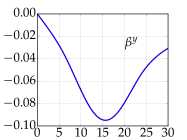
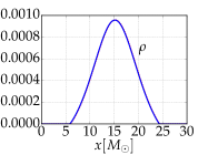
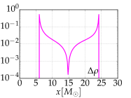
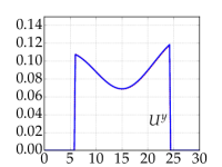
At present, however, we compute the initial data for an irrotational binary at separation of $\simeq 44.7\,{\rm km}$ by fixing $r_{s}=0.7597667$ and $d_{s}=2r_{c}=2.5$, and report in Table 2 the four different resolutions used by cocal to obtain the solutions presented here. Each symbol is explained in Table 1 and in more detail in Tsokaros et al. (2015). For simplicity, and because we are not interested in microphysical effects here, the equation of state is set to be a simple polytrope with polytropic index $\Gamma=2$ and polytropic constant $K=123.6$.

The initial data computed by lorene employs six different domains to cover the computational region around each star, with a number of collocation points for the spectral expansion given by $N_{r}\times N_{\theta}\times N_{\phi}=33\times 25\times 24$, where $N_{r}$, $N_{\theta}$, and $N_{\theta}$ denote the number of points for the radial, polar, and azimuthal directions, respectively. In our model the ratio between the star radius and the separation is roughly three, so that, according to Ref. Taniguchi and Shibata (2010), the resolution that we employ is sufficient to achieve a fractional error of $10^{-5}$ in the ADM mass comparable to the one obtained by cocal.

The physical parameters of the binary are presented in Table 3. Each star of the binary is constructed to correspond to a spherical solution of rest mass $M_{0}=1.62505$ or $M_{\rm ADM}=1.51481$, with a relative accuracy of $\mathcal{O}(10^{-6})$ in the rest mass, which is computed as

$$M_{0}=\int_{\Sigma_{t}}\rho u^{\alpha}dS_{\alpha}\,,$$ (19)

while the ADM and Komar mass are computed as

$$M_{\rm ADM} = -\frac{1}{2\pi}\int_{S_{\infty}}\partial^{i}\psi\,dS_{i}\,,$$ (20)

$$M_{\rm K} = \frac{1}{4\pi}\int_{S_{\infty}}\partial^{i}\alpha\,dS_{i}\,.$$ (21)

The surface integrals are calculated at a certain finite radius, typically around $r\sim 10^{4}\,M$, and the relative differences found between the Komar and ADM mass is of the order of $10^{-5}$ even for the cocal initial data with the coarsest resolution Hs2.0d, thus providing a simple measure of the overall error of the code. The ADM angular momentum is instead computed as

$$J=\frac{1}{8\pi}\int_{S_{\infty}}K^{a}\!{}_{b}\,\phi^{b}\,dS_{a}\,.$$ (22)

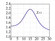
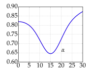
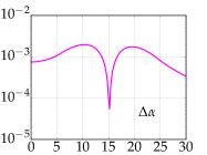
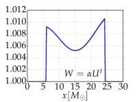
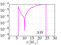
In Fig. 2 we report various quantities of the irrotational solution along the positive $x$-axis of the Cartesian grid, so that $x=0$ is the center of mass of the binary. The star of radius $R_{\rm eq}\approx 9\,M_{\odot}$ is positioned approximately at $x\approx 15\,M_{\odot}$. In both ., on the left column we plot the quantity as computed with cocal (red lines) and lorene (blue lines), relative to the Hs3.0d resolution, while on the right column we plot the relative difference

$$\Delta f:=\left|1-\frac{f_{{}_{\rm COCAL}}}{f_{{}_{\rm LORENE}}}\right|\,.$$ (23)

Going from top to bottom in Fig. 2, the quantities plotted are the metric $g_{xx}=\psi^{4}$ (note that $g_{ij}=\psi^{4}\delta_{ij}$), the lapse function $\alpha$, the $y$-component of the shift, the x$y$-component of the extrinsic curvature, and the rest mass density, while in Fig. 3, the $y$-component of the fluid velocity with respect to the Eulerian observer and the corresponding Lorentz factor.

The 4-velocity can also be written as $u^{\mu}=\alpha u^{t}(n^{\mu}+U^{\mu})$ with $n^{\mu}$, the unit normal to the hypersurface (Eulerian 4-velocity) and

$$U^{y}=\frac{1}{\alpha}\left(\frac{u^{y}}{u^{t}}+\beta^{y}\right)=\frac{\gamma^{y}_{\ \mu}u^{\mu}}{\alpha u^{t}}=\alpha\frac{\psi^{-4}\partial^{y}\Phi}{\lambda}\,,$$ (24)

where, we recall, $\lambda:=C+\omega^{i}D_{i}\Phi$. As it can be seen in Fig. 3, the difference in the computed variables between the two codes is of the order of $1\%$ or less, except for points at or near zero crossings, where the relative error, Eq. 23, produces large values.

Comparing the right columns of Figs. 2 with Fig. 6 of Ref. Uryū et al. (2012), where a similar comparison was made between cocal and kadath for black-hole binary initial data, we note that the difference between the two codes is approximately one order of magnitude larger than in Uryū et al. (2012). There are two main reasons behind this.

First, in Ref. Uryū et al. (2012) the comparison was direct in the sense that the kadath code evaluates the solution at exactly the same gridpoints used by cocal, so that no interpolation needs to be done; here, on the other hand, comparison is done after the solutions of both lorene and cocal are interpolated on the Cartesian grids. Second, and more importantly, the black-hole binary problem is scale free, thus allowing Ref. Uryū et al. (2012) to compare exactly the same physical system. This is no longer true for the neutron-star binaries that we explore here, since the two binaries have slightly different central rest-mass densities and also different separations, radii, etc. (see Table 3). This is also manifested by the fact that Figs. 2, 3 do not change considerably if we increase or decrease the cocal resolution, implying that the observed differences in the metric functions are already dominated by the intrinsic differences in the physical models considered.

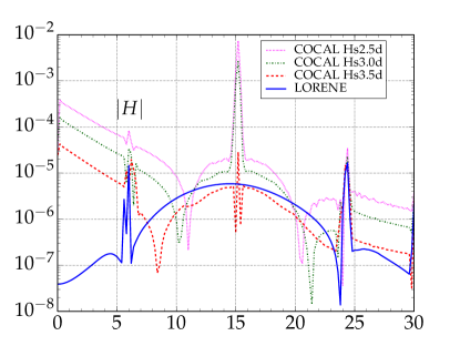
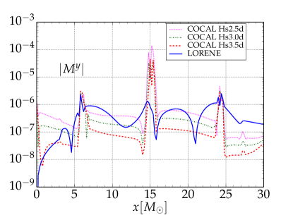
Having examined some of the representative variables of the initial dataset, we next move into an analysis of the constraint equations on the initial spacelike hypersurface. In Fig. 4 we show the residuals for both the Hamiltonian constraint equation and the $y$-component of the momentum constraint equation along the $x$-axis. Here too, $x=0$ corresponds to the center of mass of the binary with the star surface located at $x\approx 6\,M_{\odot}$, and at $x\approx 24\,M_{\odot}$. For the initial data computed with cocal we show the three highest resolutions Hs2.5d, Hs3.0d, Hs3.5d of Table 1 and note that since the star radius is $13.59\,{\rm km}$ and the number of points across the star are ${N_{r}^{\rm f}}=76,\ 100\,{\rm and}\ 150$ at these three resolutions, the spatial resolution along the $x$-axis is $179,\ 136$, and $91\,{\rm m}$, respectively.

A first reading of these plots reveals that inside the star both codes produce errors of approximately the same magnitude. For cocal, however, the Hamiltonian violations have a spike at the center of the star, i.e., at $x\approx 15\,M_{\odot}$, which converges away with resolution (cf., initial dataset Hs3.5d). This spike, which involves $\sim 4-5$ points around the center, is not a reason of major concern and for two distinct reasons. First, the localized violation is rapidly removed when the initial data is actually evolved leaving no apparent influence on the evolution (see also discussion in Section IV).

Second, as we can see from Fig. 2, the conformal factor $\psi$ is computed very accurately in the region around the stellar center; indeed, a closer inspection of the terms that produce this violation reveals that it is the result of the location of the origin of the spherical COCP, which induces local inaccuracies in the second spatial derivatives of the conformal factor, $\partial_{i}^{2}\psi$, near the stellar center. Similarly, the violations of the momentum constraint inside the star are of the same order (or even smaller) than those produced by lorene. Around the stellar surface, both codes exhibit a jump in the violations due to the existing discontinuity in the first derivatives of the matter fields. Outside the star and towards the center of mass, the cocal code produces violations that three orders of magnitude larger than lorene in the Hamiltonian constraint, but of the same order for the momentum constraint. The reason for this behaviour is probably to be found in the resolution of the radial grid, since in that region we have an increasing step of $\delta x$. We plan to study the source of this error in the future, by modifying the grid structure there. From the opposite side of the star and moving towards spatial infinity, again we have a reasonable agreement between the three sets of initial data. It is also important to notice that the cocal violations converge away with the expected second-order accuracy of the finite-difference scheme.

IV Impact on the evolutions of different initial-data solvers

In order to evolve the initial datasets introduced in the previous section, we have used the high-order evolution code WhiskyTHC Radice et al. (2014a, b, 2015), which solves the equations of general-relativistic hydrodynamics in the Valencia formulation Banyuls et al. (1997) using a finite-difference scheme that reconstructs the fluxes in local-characteristic variables using a high-order reconstruction scheme (MP5 Suresh and Huynh (1997)). In these simulations, we also employed a positivity preserving limiter, which is crucial to treat properly the low-density regions of the flow Radice et al. (2014a). The evolution of the spacetime is provided by the McLachlan code Brown et al. (2009), which solves a conformal-traceless “$3+1$” formulation of the Einstein equations either in the BSSNOK Nakamura et al. (1987); Shibata and Nakamura (1995); Baumgarte and Shapiro (1999) or in the CCZ4 form Alic et al. (2012); we have here employed the BSSNOK formulation, leaving to future work the investigation with the CCZ4 formulation. The McLachlan code is part of the open source software framework Einstein Toolkit Löffler et al. (2012); Einstein Toolkit Website , which is based on the cactus Cactus Website computational toolkit. We use a fourth-order finite differencing and the very robust Gamma-driver shift condition together with the ’$1+\log$’ slicing, which have been shown to be numerically well-behaved for spacetimes describing both isolated and neutron-star binaries Baiotti et al. (2005); Baiotti and Rezzolla (2006); Baiotti et al. (2008).

Figure 5: Logarithmic violations of the constraint equations shown at three different times in the different columns: initial time ($t=0$), just after the beginning of the evolution ($t=30.72\,M_{\odot}$), and one orbit later ($t=660.48\,M_{\odot}$). From top to bottom, the first row shows the violations of the Hamiltonian constraint on the $(x,y)$ plane from cocal, while the second row the corresponding violations from lorene. The third and fourth rows show the violations of the $y$-component of the momentum constraint from cocal and lorene, respectively. Note that all panels show data on three finest levels of refinement, with two borders clearly visible. The bounding box in the $(x,y)$ plane encompassing each of the panels spans roughly the range $[0,50]\times[-25,25]\,M_{\odot}$. The oval shape indicates the neutron star surface at every moment.

In particular, we use for these simulations a computational domain in which $0<x,z\leq 1024\,M_{\odot}$ and $-1024\,M_{\odot}\leq y\leq 1024\,M_{\odot}$, i.e.,  we assume $\pi$ symmetry along the $(x,z)$ plane and reflection symmetry on the $(x,y)$ plane. It is important to remark that placing the outer boundary at a sufficiently large radius is crucial to avoid that spurious and constraint-violating reflections from the outer boundaries spoil the convergence order; for example, we have experienced that having a computational domain with outer boundary at $512\,M_{\odot}\simeq 755\,{\rm km}$, which is quite common for neutron-star binary simulations Rezzolla and Takami , would not yield convergence waveforms.

An adaptive mesh-refinement grid (AMR) hierarchy is provided by the carpet driver Schnetter et al. (2004); Carpet Website , and we use six levels of refinement, the finest of which has three different resolutions: low (L), medium (M), and high (H). These three resolutions correspond respectively to spatial mesh spacings of $h=0.2,\ 0.133,\ 0.1\,M_{\odot}\simeq 295,\ 197,\ 148\,{\rm m}$, or, equivalently, to $80,\ 120,\,{\rm and}\ 160$ cells along the $x$-axis for the coarsest grid. See Table 4 for more details on this grid hierarchy.

Level	AMR Box Extent			Mesh Spacing
	$x$	$y$	$z$	$h$
$0$	$[0,1024]$	$[-1024,1024]$	$[0,1024]$	$3.2$
$1$	$[0,240]$	$[-240,240]$	$[0,240]$	$1.6$
$2$	$[0,120]$	$[-120,120]$	$[0,120]$	$0.8$
$3$	$[0,64]$	$[-64,64]$	$[0,48]$	$0.4$
$4$	$[0,40]$	$[-40,40]$	$[0,22]$	$0.2$
$5$	$[0,30]$	$[-30,30]$	$[0,11]$	$0.1$

Table 4: AMR grid hierarchy: reported are the boxes’ extents along the $x$, $y$ and $z$ directions, which reflect whether the symmetry conditions imposed on them, i.e., $\pi$-symmetry along the $x$ coordinate at $x=0$ (on the $(y,z)$ plane); reflection symmetry along the $z$ coordinate at $z=0$, i.e., on the $(x,y)$ equatorial plane. The grid hierarchy was kept fixed throughout the simulation for each one of the different simulations. The mesh spacings listed on the last column are the ones used for the highest-resolution simulation.

The initial data, computed either with lorene and cocal (for the latter we use the Hs3.5d dataset) is then evolved with a Courant factor set to to $0.3$. We note that we reset the shift vector to zero at the start of each evolution, i.e., we do not use the shift as provided be the initial data codes. The two stars inspiral for about three orbits (i.e., approximately seven gravitational-wave cycles) and then merge. Because the initial masses have been chosen to be sufficiently large, the merger leads to a prompt collapse to a black hole surrounded by an accretion torus Baiotti et al. (2008).

Figure 6: Constraint violation $L_{2}$ norms for cocal and lorene as a function of time. The first row shows the Hamiltonian constraint, while the second row represents the $y$-component of the momentum constraint. Each color refers to a given resolution for the evolution grid: low (red), medium (green), and high (blue).

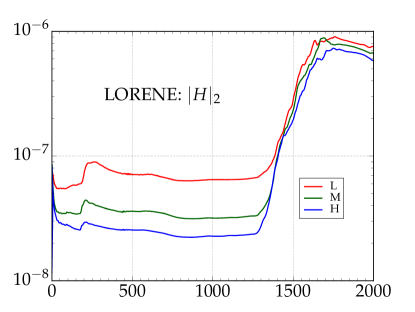
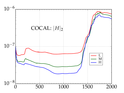
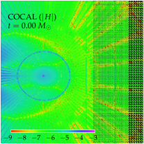
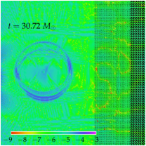
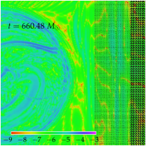
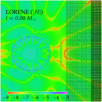
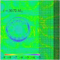
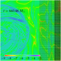
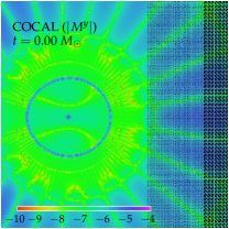
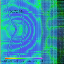
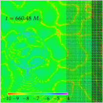
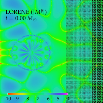
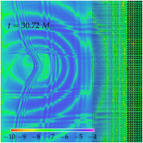
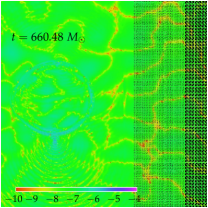
A more complete picture of the constraint violations as a function of time is shown in Fig. 5, where each panel shows the constraint violations in the equatorial plane, or $(x,y)$ plane, of the binary, focusing on the region from the center of mass (middle of left side on each panel) to approximately six neutron-star radii. From top to bottom, the first row represents cocal Hs3.0d initial data, while the second row shows the lorene Hamiltonian violations at three different times: at $t=0$, which corresponds to the initial data, just after the simulation is launched, at $t=30.72\,M_{\odot}$, and after one orbit, at $t=660.48\,M_{\odot}$. When considering the properties of the initial data, it is possible to note the characteristic spherical-coordinates pattern of cocal, while in case of lorene data, one has a wavy kind of structure which reflects the spectral methods used. The surface of the neutron star is easily noticeable as violations of the constraints tend to create a discontinuity there. Also visible is the increase of cocal’s violations towards the center of mass as was seen in Fig. 4. Apparently these violations exist in the region around the $(y,z)$ plane close to the center of mass. The small spike of violations at the center of the neutron star is also visible.

Soon after the beginning of the evolution, at $t=30.72\,M_{\odot}$ (middle column), the stars have rotated of about one degree and the violations of both codes become very similar both inside the star as well as near the center of mass. This tendency continues one orbit afterwards (third column) at $t=660.48\,M_{\odot}$ up until the merger. In the third and fourth rows, we show the momentum violations for cocal and lorene, respectively. Again the characteristic patterns of both codes are visible in the initial data first column, with cocal having less violations inside and around the star. As the binary evolves differences are washed out and both codes produce similar behaviours.

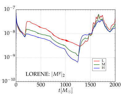
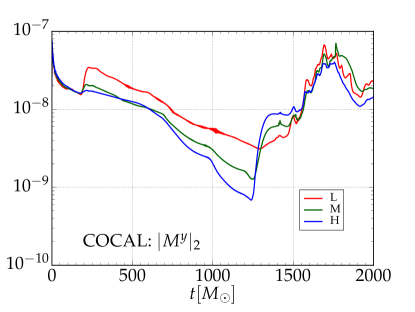
Up until now all convergence analysis has been done with respect to the resolution of the initial data. In what follows we fix the initial data (Hs3.5d for cocal) and perform a convergence analysis with respect to the resolution of the evolution code. In Fig. 6, we monitor the $L_{2}$ norm indicator for the Hamiltonian (first row) and $y$-component of the momentum constraint (second row). It is defined as

$$|f|_{2}:=\sqrt{\frac{1}{N}\sum_{i=1}^{N}|f_{i}|^{2}}\,,$$ (25)

where $N=N_{r}\times N_{\theta}\times N_{\phi}$ is the total number of points. Merger happens at approximately $1500\,M_{\odot}$ or $8\,{\rm ms}$.

Every plot has three solid lines that correspond to the three different evolution resolutions: red is for low, green is for medium, and blue is for high, with outer boundaries at $1024\,M_{\odot}$ as stated earlier. A first feature to be noticed in these plots is the presence of a local maximum around $180\,M_{\odot}$, and the behavior of the violations until that time. It is possible to see in Fig. 6 that this maximum is reduced as the resolution of the evolution increases and that its position in time changes as the position of the second AMR refinement boundary is varied. Together, these considerations clearly indicate that the first local maximum in the constraint violations is simply due to the position of the second AMR box and, albeit, annoying has a clear origin and is not particularly harmful for the subsequent evolution.

A second feature to notice when considering the constraint violations in the time interval $0<t<180\,M_{\odot}$ is that although the ones coming from the Hamiltonian equation scale according to the resolution (except for an initial interval $0<t<50\,M_{\odot}$), this is not happening for the momentum-constraint equation. There, the violations monotonically decrease until the starting of the ”bump” at $t=180\,M_{\odot}$, and increasing the resolution does not affect them. Since the initial data computed with cocal and lorene are already at high resolution, and since for $t=0$ the violations are approximately more than five times the ones at $t=180\,M_{\odot}$, we believe that this behavior is caused by inaccuracies inherent in the initial data formalism, like the omission of certain equations or terms in the Euler and the gravitational field equations. After a certain time ($180\,M_{\odot}$ in our case) these violations are washed out and then evolution errors scale accordingly.

In addition to the $L_{2}$ norm shown here, we have also computed and studied the behaviour of the $L_{1}$ norm (i.e., $|f|_{1}:=\sum_{i=1}^{N}|f_{i}|/N$) and of the $L_{\infty}$ norm (i.e., $|f|_{\infty}:=\max_{i}\{|f_{i}|\}$). More specifically, the $L_{1}$ norm is of the order $\lesssim 10^{-8}$ for all the resolutions considered, both for the cocal and for the lorene initial data, while the $L_{\infty}$ norm is the largest of all, with values of the order of $\lesssim 10^{-6}$. Also this quantity, however, shows a clear convergence scaling in the Hamiltonian violations. Overall, it is evident that the behavior of the evolution of the constraint violations is extremely similar both for cocal as well as for lorene initial data.

Figure 7: First row: real part of $(\Psi_{4})_{22}$ extracted at $\bar{r}=450\,M_{\odot}$ as a function of the retarded time for both cocal Hs3.5d (left panel) and lorene (right panel) initial data and for the three evolution resolutions (L, M, H). On each plot with dashed line we denote the evolution with the highest resolution of the other code initial dataset so that the dephasing between the two datasets to become apparent. Second row: dephasing between different resolutions and the rescaled dephasing between the high and medium resolution assuming a convergence order $p=2.71$. The left panel is for cocal, while right one is for lorene. Third row: relative phase difference for the $\ell=m=2$ mode of $\Psi_{4}$ with respect to the Richardson-extrapolated value (computed assuming a convergence order of $p=2.71$).

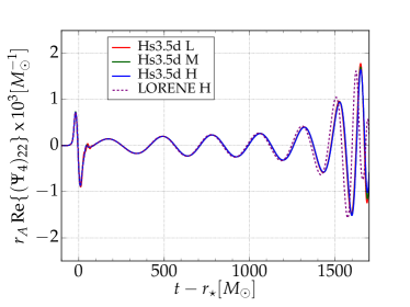
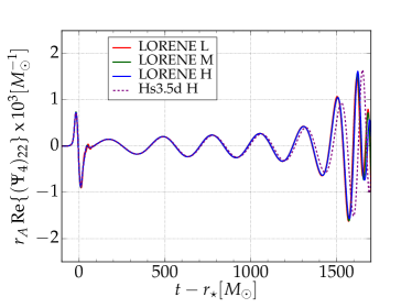
One of the main goals in this work is to estimate the impact that slightly different initial data can have on the observed gravitational-wave signal. It is well known that the Einstein equations are highly nonlinear and is therefore possible that even minute differences in the initial data can result into large and indeed measurable differences in the radiated quantities. The ability of measuring how large this impact is of course essential to weigh it in in the overall budget of numerical-relativity calculations and hence to measure how the extraction of physical parameters of the sources can be affected. Hence, we next concentrate here on the gravitational-wave emission on the $\ell=m=2$ mode of the Weyl scalar $\Psi_{4}$ which we extract at $\bar{r}=450\,M_{\odot}$

$$(\Psi_{4})_{22}=A(t)e^{i\phi(t)}\,.$$ (26)

The real part of $(\Psi_{4})_{22}$ with respect to the retarded time $t-r_{\star}$, is plotted in the top row of Fig. 7, where

$$r_{\star}:=r_{A}+2M_{\rm ADM}\ln\left({r_{A}}/{2M_{\rm ADM}}-1\right)\approx 478.8\,M_{\odot}\,,$$ (27)

is the tortoise radius and $r_{A}:=\bar{r}(1+M_{\rm ADM}/2\bar{r})^{2}$ is the approximated areal radius.

Figure 8: Convergence order $p$ as a function of time as computed by Eq. 28 for cocal (top panel) and lorene (bottom panel) initial data. The average values for cocal (lorene), i.e., $p=2.71\pm 0.27(2.77\pm 0.24)$, are computed as arithmetic averages over the time interval $[650,1500]\,M_{\odot}$ where outlier data points, $p<1$ and $p>4$ are excluded from the average and represent the uncertainty range.

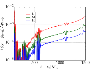
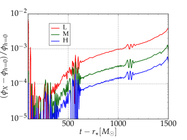
The left panel in the top row of Fig. 7 refers to the cocal Hs3.5d initial data and we report the waveforms as computed at the the three different resolutions L (red line), M (green line) and H (blue line), which, we recall, are relative to spatial mesh spacings of $0.2,\ 0.1333,\ 0.1\,M_{\odot}$ on the finest grid. Note that at these resolutions the differences among the various waveforms are extremely small, both in phase and in amplitude and one needs to zoom-in in the figure to appreciate them. Similar waveforms are shown in the right panel in the top row of Fig. 7, which instead refers to the lorene initial data. On each of these plots we also include a dashed magenta line with the highest resolution run of the other initial dataset in order to emphasize the dephasing that is instead observed when comparing the two initial datasets.

Figure 9: Difference between the Richardson-extrapolated phases for cocal and lorene initial data using the three resolutions L, M, and H.

This dephasing observed in the top row of Fig. 7 is reminiscent of the behaviour observed in Radice et al. (2014b), where a comparison between two evolution codes of different convergence order, Whisky Baiotti and Rezzolla (2006); Baiotti et al. (2008) and WhiskyTHC, has been made. In that work, it was shown that given the exactly same initial data, a second-order evolution code (Whisky) produces a significant phase difference for the gravitational wave at different resolutions. This phase difference was as large as $\sim 2$ radians between a low and a high-resolution simulation. When the same experiment was repeated using the higher-order WhiskyTHC code the dephasing between different resolutions became as small as $\sim 0.6$ radians. Here, the evolution runs have been done with WhiskyTHC only and the small differences in phase are due uniquely to small differences in the initial datasets. In other words, the evolution of the two slightly different initial datasets resembles the dephasing measured when using evolution codes with different orders of accuracy.

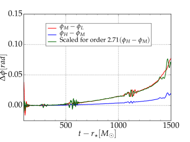
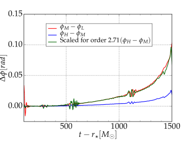
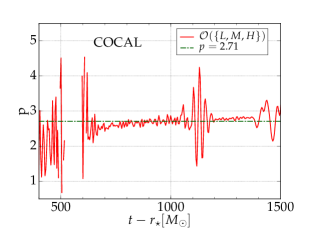
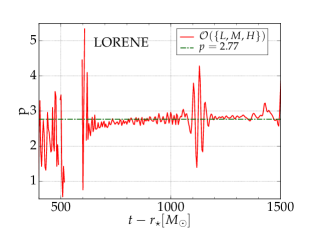
To gain a better understanding of the dephasing and to compare the convergence properties for both sets of initial data, we report the change $\Delta\phi$ between medium and low, as well as the high and medium resolutions in the middle row of Fig. 7. The left plot refers to the cocal initial data, while the right plot to the lorene initial data. Also plotted is the rescaled $\Delta\phi$ for the high-minus-medium resolution, and after employing a convergence order of $p=2.71$ (see Fig. 8 and the discussion below). This exponent $p$ is a genuine measure of the convergence order of our code and we believe similar measurements should accompany any work reporting high-quality gravitational waveforms. Here, $p$ has been computed by solving the equation Rezzolla and Zanotti (2013); Radice et al. (2014a)

$$\frac{\phi_{h_{1}}-\phi_{h_{2}}}{\phi_{h_{2}}-\phi_{h_{3}}}\ =\ \frac{h_{1}^{p}-h_{2}^{p}}{h_{2}^{p}-h_{3}^{p}}\ ,$$ (28)

where $(h_{1},h_{2},h_{3})=(0.2,0.1333,0.1)$ are the intervals of the three resolutions L, M, and H employed. Note that because $p$ is a function of time (see Fig. 8), the value reported refers to the average over time of all convergence orders, after discarding an initial noisy time interval. In this way, we obtain $p=2.71\pm 0.27$ for the cocal initial data and essentially the same value, i.e., $p=2.77\pm 0.24$, for the lorene initial data. A convergence order of this magnitude is consistent with previous studies Radice et al. (2014b) of binaries at close separations. At the last row of Fig. 7 (again left plot refers to cocal while right plot to lorene initial data) we calculate the relative difference between the Richardson-extrapolated phase for the three resolutions used. The value at infinite resolution ($h=0$) is calculated from Eq. (28) by setting, for example $h_{1}=0$, and solving for $\phi_{h_{1}}$, using the previously calculated convergence order $p=2.71$, this is computed as

$$\phi_{h=0}=\phi_{h_{2}}+\frac{\phi_{h_{2}}-\phi_{h_{3}}}{({h_{3}}/{h_{2}})^{p}-1}\,.$$ (29)

In all cases, although the overall behavior looks extremely similar the significant dephasing can result to different observables.

In Fig. 9 we plot the difference between the Richardson-extrapolated ($h=0$) phases of the cocal and lorene initial data using the L, M, H resolutions. As it is quite apparent, even after approximately one orbit, the evolutions resulting from cocal and lorene initial data differ by as much as $0.1$ radians and the difference is approximately $0.5$ radians at merger time. Stated differently, despite employing initial data referring to essentially the same physical binary and computed by two highly accurate numerical codes yielding global (local) differences that are $\lesssim 0.02\%\ (1\%)$, the extrapolated gravitational-wave phases at the merger time can differ by $\sim 0.5$ radians already after $\sim 3$ orbits. Considering that these results have been obtained after using rather high spatial resolutions, we believe that the use of a high-order numerical code such as WhiskyTHC has been crucial in bringing out these differences.

V Conclusions

We have presented the first evolutions of our newly constructed initial-data code cocal Tsokaros et al. (2015), and performed an accurate study on the role that slightly different initial data play on the evolution of neutron-star binaries. The coc$2$cac driver, that enables communication with existing evolution codes in cactus toolkit, was presented and a detailed converge analysis both with respect to the initial data itself, as well as with respect to the WhiskyTHC evolution code was performed for the case of irrotational neutron-star binaries separated at $45\,{\rm km}$. In addition, for benchmark purposes regarding future spinning simulations, we have also examined a corotating solution at $45\,{\rm km}$.

Our main goals in this work have been, on the one hand, to validate the accuracy of the initial data constructed by this new initial data code and, on the other hand, to estimate potential differences on the gravitational-wave signal as it is produced by different initial data codes. For this purpose, we have used the widely used, open-source code lorene and have carried out a close comparison for the initial data computed with the codes when considering the same physical binary. For the first time, we have also explored the impact that the minute differences in the two initial-datasets have on the extrapolated gravitational-wave signal.

In this way, we have found that although the initial data between the the two initial-data codes have global (local) differences that are $\lesssim 0.02\%\ (1\%)$, the extrapolated gravitational-wave signal at the merger time and after about three orbits can have a dephasing of half a radian. This is an alarming reminder of the care that needs to be paid when comparisons are performed between results that start from slightly different initial data or when the initial data errors are not properly taken into account in the simulation error budget.

Appendix A Pointwise comparison of corotating solutions

Figure 10: The same as in Fig. 2 but a corotating binary. The dashed green line refers to the irrotational solution in Fig. 2, and which has a very similar mass (cf., Tables 3 and 5).

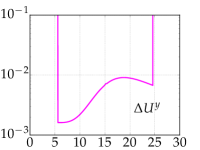
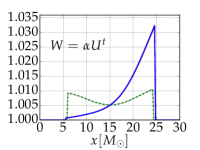
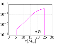
Although corotating solutions are not considered as physically realistic because the shear viscosity in neutron stars is too small to guarantee that this tidal coupling takes place Kochanek (1992); Bildsten and Cutler (1992), in this appendix we calculate a corotating neutron-star binary at $45\,{\rm km}$ and compare our solutions pointwise with a solution calculated from lorene. The reason is that corotating binaries are easier to calculate, since the fluid rotates at the same angular velocity as the binary, and hence they can be considered as a benchmark for error estimation in binary calculations. Also, since they represent the simplest spinning-binary configuration, they provide insight for the magnitude of the error introduced by more complicated arbitrary spinning solutions.

Figure 11: Hamiltonian (top) and momentum violations (bottom) for the $y$-component of the shift ($\beta^{y}$) along the $x$-axis for corotating (solid lines) neutron-star binaries. Dashed lines are the corresponding irrotational cocal and lorene violations as appear in Fig. 4. The origin $x=0$ corresponds to the center of mass of the binary with the surface of the star to be located at $x\approx 6\,M_{\odot}$, and at $x\approx 24\,M_{\odot}$. Grid parameters used in cocal are those of Hs3.0d.

To enforce corotation, we set $V^{\alpha}=0$ and the Eulerian velocity is then given by

$$U^{i}=\frac{\omega^{i}}{\alpha}\,.$$ (30)

We only consider the Hs3.0d resolution and the main physical quantities for both cocal and lorene are reported in Table 5. Note that the central rest-mass density is smaller than for the irrotational binary, while the ADM mass and angular momentum being slightly larger. This is simply due to the stellar rotation, that tends to stabilize the binary by including rotational kinetic energy.

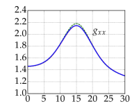
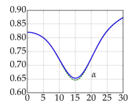
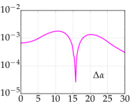
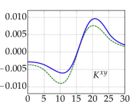
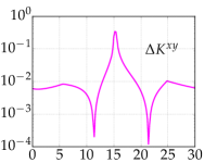
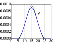
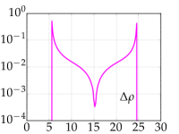
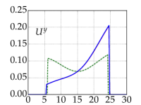
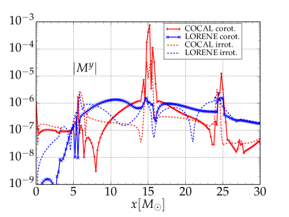
In Fig. 10 we plot along the positive $x$-axis the conformal factor, the lapse function $\alpha$, the $xy$-component of the extrinsic curvature, the rest-mass density $\rho$, the $y$-component of the velocity and the Lorentz factor for both cocal (red lines) and lorene (blue lines) solutions. As in Fig. 2, $x=0$, corresponds to the center of mass of the system. Also plotted with a dashed green line is the corresponding irrotational solution as reported in Fig. 2. A rapid inspection shows that the conformal factor and the lapse are slightly smaller inside the star, while the extrinsic curvature increases (decreases) towards the outer (inner) part of the star. Also the velocity profile has much larger values in the outer parts of the star (i.e., those farther away from the center of mass) and this is the an obvious manifestation of the large spin component introduced by the corotation and that is reflected in the Lorentz factor too. Overall, and as for the irrotational case, also here the differences between the two datasets are $\lesssim 1\%$.

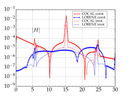
In Fig. 11 we plot the constraint violations as we have done in Fig. 4 for the irrotational binaries. Only one resolution for cocal, the Hs3.0d, is plotted, together with the corresponding violations from the irrotational solutions (shown with dashed lines; cf., Fig. 4), that are shown for comparison.

The comparison with the results from lorene shows a very similar behaviour to the one already discussed for the irrotational case: the Hamiltonian violations are larger but the violations of the momentum constraint smaller. Comparing instead the cocal irrotational data with the the corotating cases, we see that the violations are larger in the corotating binary. Hence, although the fluid formulation is significantly more complicated in the case of irrotational binaries, the large rotation present in corotating binaries induces a small amount of extra violations for both finite-difference and spectral-method codes. We expect that a similar behavior will be shown also by neutron-star binaries with arbitrary spins.

	lorene	cocal
$M_{0}$	$1.62504$	$1.62505$
$M_{\rm ADM}$	$3.00274$	$3.00275$
$M_{\rm K}$	$-$	$3.00243$
$\rho_{c}\ (\times 10^{-4})$	$9.04601$	$9.04969$
$J_{\rm ADM}$	$9.76287$	$9.75909$
$\Omega\ [{\rm rad/sec}]$	$1857.82$	$1848.84$
$d_{s}\ [{\rm km}]$	$44.731$	$44.736$
$R_{\rm eq}\ [{\rm km}]$	$14.193$	$14.181$

Table 5: Physical parameters for a corotating binary computed with either cocal or lorene (see Table 3 for a description of the various quantities). The resolution used for cocal is Hs3.0d of Table 1, except for parameter $r_{s}=0.7925$ in order to create a binary at separation $44.7\,{\rm km}$.

References

- Abbott et al. (2016) B. P. Abbott, R. Abbott, T. D. Abbott, M. R. Abernathy, F. Acernese, K. Ackley, C. Adams, T. Adams, P. Addesso, R. X. Adhikari, and et al., Phys. Rev. Lett. 116, 061102 (2016), arXiv:1602.03837 [gr-qc] .
- Abramovici et al. (1992) A. A. Abramovici, W. Althouse, R. P. Drever, Y. Gursel, S. Kawamura, F. Raab, D. Shoemaker, L. Sievers, R. Spero, K. S. Thorne, R. Vogt, R. Weiss, S. Whitcomb, and M. Zuker, Science 256, 325 (1992).
- Accadia et al. (2011) T. Accadia et al., Class. Quantum Grav. 28, 114002 (2011).
- Kuroda and LCGT Collaboration (2010) K. Kuroda and LCGT Collaboration, Class. Quantum Grav. 27, 084004 (2010).
- Aso et al. (2013) Y. Aso, Y. Michimura, K. Somiya, M. Ando, O. Miyakawa, T. Sekiguchi, D. Tatsumi, and H. Yamamoto, Phys. Rev. D 88, 043007 (2013), arXiv:1306.6747 [gr-qc] .
- Punturo et al. (2010) M. Punturo et al., Class. Quantum Grav. 27, 084007 (2010).
- Narayan et al. (1992) R. Narayan, B. Paczynski, and T. Piran, Astrophysical Journal, Letters 395, L83 (1992), astro-ph/9204001 .
- Eichler et al. (1989) D. Eichler, M. Livio, T. Piran, and D. N. Schramm, Nature 340, 126 (1989).
- Rezzolla et al. (2011) L. Rezzolla, B. Giacomazzo, L. Baiotti, J. Granot, C. Kouveliotou, and M. A. Aloy, Astrophys. J. Letters 732, L6 (2011), arXiv:1101.4298 [astro-ph.HE] .
- Bartos et al. (2013) I. Bartos, P. Brady, and S. Marka, Class. Quant. Grav. 30, 123001 (2013), arXiv:1212.2289 [astro-ph.CO] .
- Berger (2014) E. Berger, Annual Review of Astron. and Astrophys. 52, 43 (2014), arXiv:1311.2603 [astro-ph.HE] .
- Lattimer and Schramm (1974) J. M. Lattimer and D. N. Schramm, Astrophysical Journal, Letters 192, L145 (1974).
- Li and Paczynski (1998) L.-X. Li and B. Paczynski, Astrophys. J. 507, L59 (1998), arXiv:astro-ph/9807272 [astro-ph] .
- Tanvir et al. (2013) N. R. Tanvir, A. J. Levan, A. S. Fruchter, J. Hjorth, R. A. Hounsell, K. Wiersema, and R. L. Tunnicliffe, Nature 500, 547 (2013), arXiv:1306.4971 [astro-ph.HE] .
- Berger et al. (2013) E. Berger, W. Fong, and R. Chornock, Astrophys. J. 774, L23 (2013), arXiv:1306.3960 [astro-ph.HE] .
- Tanaka and Hotokezaka (2013) M. Tanaka and K. Hotokezaka, Astrophys. J. 775, 113 (2013), arXiv:1306.3742 [astro-ph.HE] .
- Rosswog et al. (2014) S. Rosswog, O. Korobkin, A. Arcones, F.-K. Thielemann, and T. Piran, Mon. Not. R. Astron. Soc. 439, 744 (2014), arXiv:1307.2939 [astro-ph.HE] .
- Sekiguchi et al. (2015) Y. Sekiguchi, K. Kiuchi, K. Kyutoku, and M. Shibata, Phys. Rev. D 91, 064059 (2015), arXiv:1502.06660 [astro-ph.HE] .
- Radice et al. (2016) D. Radice, F. Galeazzi, J. Lippuner, L. F. Roberts, C. D. Ott, and L. Rezzolla, ArXiv e-prints (2016), arXiv:1601.02426 [astro-ph.HE] .
- Shibata and Uryū (2000) M. Shibata and K. Uryū, Phys. Rev. D 61, 064001 (2000), gr-qc/9911058 .
- Baiotti et al. (2008) L. Baiotti, B. Giacomazzo, and L. Rezzolla, Phys. Rev. D 78, 084033 (2008), arXiv:0804.0594 [gr-qc] .
- Sekiguchi et al. (2011a) Y. Sekiguchi, K. Kiuchi, K. Kyutoku, and M. Shibata, Phys. Rev. Lett. 107, 211101 (2011a), arXiv:1110.4442 [astro-ph.HE] .
- Takami et al. (2015) K. Takami, L. Rezzolla, and L. Baiotti, Phys. Rev. D 91, 064001 (2015), arXiv:1412.3240 [gr-qc] .
- Sekiguchi et al. (2011b) Y. Sekiguchi, K. Kiuchi, K. Kyutoku, and M. Shibata, Phys. Rev. Lett. 107, 051102 (2011b), arXiv:1105.2125 [gr-qc] .
- Galeazzi et al. (2013) F. Galeazzi, W. Kastaun, L. Rezzolla, and J. A. Font, Phys. Rev. D 88, 064009 (2013), arXiv:1306.4953 [gr-qc] .
- Anderson et al. (2008) M. Anderson, E. W. Hirschmann, L. Lehner, S. L. Liebling, P. M. Motl, D. Neilsen, C. Palenzuela, and J. E. Tohline, Phys. Rev. Lett. 100, 191101 (2008), arXiv:0801.4387 [gr-qc] .
- Liu et al. (2008) Y. T. Liu, S. L. Shapiro, Z. B. Etienne, and K. Taniguchi, Phys. Rev. D 78, 024012 (2008).
- Giacomazzo et al. (2009) B. Giacomazzo, L. Rezzolla, and L. Baiotti, Mon. Not. R. Astron. Soc. 399, L164 (2009).
- Kiuchi et al. (2014) K. Kiuchi, K. Kyutoku, Y. Sekiguchi, M. Shibata, and T. Wada, Phys. Rev. D 90, 041502 (2014), arXiv:1407.2660 [astro-ph.HE] .
- Dionysopoulou et al. (2015) K. Dionysopoulou, D. Alic, and L. Rezzolla, Phys. Rev. D 92, 084064 (2015), arXiv:1502.02021 [gr-qc] .
- Uryū et al. (2012) K. Uryū, A. Tsokaros, and P. Grandclement, Phys. Rev. D86, 104001 (2012), arXiv:1210.5811 [gr-qc] .
- Tsokaros et al. (2015) A. Tsokaros, K. Uryū, and L. Rezzolla, Phys. Rev. D 91, 104030 (2015), arXiv:1502.05674 [gr-qc] .
- (33) Lorene Website, “LORENE Langage Objet pour la RElativité NumériquE,” http://www.lorene.obspm.fr.
- Grandclement (2010) P. Grandclement, J. Comput. Phys. 229, 3334 (2010), arXiv:0909.1228 [gr-qc] .
- Tichy (2009) W. Tichy, Class. Quant. Grav. 26, 175018 (2009), arXiv:0908.0620 [gr-qc] .
- Tichy (2012) W. Tichy, Phys. Rev. D 86, 064024 (2012), arXiv:1209.5336 [gr-qc] .
- (37) SpEC Website, “SpEC Spectral Einstein Code,” http://www.black-holes.org/SpEC.html.
- East et al. (2012) W. E. East, F. M. Ramazanoǧlu, and F. Pretorius, Phys. Rev. D 86, 104053 (2012), arXiv:1208.3473 [gr-qc] .
- Brügmann et al. (2008) B. Brügmann, J. A. González, M. Hannam, S. Husa, U. Sperhake, and W. Tichy, Phys. Rev. D 77, 024027 (2008), gr-qc/0610128, gr-qc/0610128 .
- Baumgarte et al. (1998) T. W. Baumgarte, G. B. Cook, M. A. Scheel, S. L. Shapiro, and S. A. Teukolsky, Phys. Rev. D 57, 7299 (1998), gr-qc/9709026 .
- Kochanek (1992) C. S. Kochanek, Astrophys. J. 398, 234 (1992).
- Bildsten and Cutler (1992) L. Bildsten and C. Cutler, Astrophys. J. 400, 175 (1992).
- Kyutoku et al. (2014) K. Kyutoku, M. Shibata, and K. Taniguchi, Phys. Rev. D 90, 064006 (2014), arXiv:1405.6207 [gr-qc] .
- Moldenhauer et al. (2014) N. Moldenhauer, C. M. Markakis, N. K. Johnson-McDaniel, W. Tichy, and B. Brügmann, Phys. Rev. D 90, 084043 (2014), arXiv:1408.4136 [gr-qc] .
- Bernuzzi et al. (2014) S. Bernuzzi, T. Dietrich, W. Tichy, and B. Brügmann, Phys. Rev. D 89, 104021 (2014), arXiv:1311.4443 [gr-qc] .
- Kastaun et al. (2013) W. Kastaun, F. Galeazzi, D. Alic, L. Rezzolla, and J. A. Font, Phys. Rev. D 88, 021501 (2013), arXiv:1301.7348 [gr-qc] .
- Tsatsin and Marronetti (2013) P. Tsatsin and P. Marronetti, Phys. Rev. D 88, 064060 (2013).
- Dietrich et al. (2015) T. Dietrich, N. Moldenhauer, N. K. Johnson-McDaniel, S. Bernuzzi, C. M. Markakis, B. Brügmann, and W. Tichy, Phys. Rev. D 92, 124007 (2015), arXiv:1507.07100 [gr-qc] .
- Tacik et al. (2015) N. Tacik, F. Foucart, H. P. Pfeiffer, R. Haas, S. Ossokine, J. Kaplan, C. Muhlberger, M. D. Duez, L. E. Kidder, M. A. Scheel, and B. Szilágyi, Phys. Rev. D 92, 124012 (2015), arXiv:1508.06986 [gr-qc] .
- Uryū and Tsokaros (2012) K. Uryū and A. Tsokaros, Phys. Rev. D 85, 064014 (2012), arXiv:1108.3065 [gr-qc] .
- Tsokaros and Uryū (2012) A. Tsokaros and K. Uryū, Journal of Engineering Mathematics 82, 133 (2012).
- Radice et al. (2014a) D. Radice, L. Rezzolla, and F. Galeazzi, Mon. Not. R. Astron. Soc. L. 437, L46 (2014a), arXiv:1306.6052 [gr-qc] .
- Radice et al. (2014b) D. Radice, L. Rezzolla, and F. Galeazzi, Class. Quantum Grav. 31, 075012 (2014b), arXiv:1312.5004 [gr-qc] .
- Radice et al. (2015) D. Radice, L. Rezzolla, and F. Galeazzi, Numerical Modeling of Space Plasma Flows ASTRONUM-2014, Astronomical Society of the Pacific Conference Series, 498, 121 (2015), arXiv:1502.00551 [gr-qc] .
- Baiotti et al. (2010) L. Baiotti, M. Shibata, and T. Yamamoto, Phys. Rev. D 82, 064015 (2010), arXiv:1007.1754 [gr-qc] .
- Read et al. (2013) J. S. Read, L. Baiotti, J. D. E. Creighton, J. L. Friedman, B. Giacomazzo, K. Kyutoku, C. Markakis, L. Rezzolla, M. Shibata, and K. Taniguchi, Phys. Rev. D 88, 044042 (2013), arXiv:1306.4065 [gr-qc] .
- (57) Cactus Website, “Cactus Computational Toolkit,” http://www.cactuscode.org.
- Rezzolla and Zanotti (2013) L. Rezzolla and O. Zanotti, Relativistic Hydrodynamics (Oxford University Press, Oxford, UK, 2013).
- Löffler et al. (2012) F. Löffler, J. Faber, E. Bentivegna, T. Bode, P. Diener, R. Haas, I. Hinder, B. C. Mundim, C. D. Ott, E. Schnetter, G. Allen, M. Campanelli, and P. Laguna, Class. Quantum Grav. 29, 115001 (2012), arXiv:1111.3344 [gr-qc] .
- (60) Einstein Toolkit Website, “Einstein Toolkit: Open Software for Relativistic Astrophysics,” http://einsteintoolkit.org.
- Tsokaros and Uryū (2007) A. A. Tsokaros and K. Uryū, Phys. Rev. D 75, 044026 (2007).
- Huang et al. (2008) X. Huang, C. Markakis, N. Sugiyama, and K. Uryū, Phys. Rev. D78, 124023 (2008), arXiv:0809.0673 [astro-ph] .
- Uryū et al. (2016) K. Uryū, A. Tsokaros, F. Galeazzi, H. Hotta, M. Sugimura, K. Taniguchi, and S. Yoshida, Phys. Rev. D93, 044056 (2016).
- Taniguchi and Shibata (2010) K. Taniguchi and M. Shibata, Astrophys. J., Supp. 188, 187 (2010), arXiv:1005.0958 [astro-ph.SR] .
- Banyuls et al. (1997) F. Banyuls, J. A. Font, J. M. Ibáñez, J. M. Martí, and J. A. Miralles, Astrophys. J. 476, 221 (1997).
- Suresh and Huynh (1997) A. Suresh and H. T. Huynh, Journal of Computational Physics 136, 83 (1997).
- Brown et al. (2009) D. Brown, P. Diener, O. Sarbach, E. Schnetter, and M. Tiglio, Phys. Rev. D 79, 044023 (2009), arXiv:0809.3533 [gr-qc] .
- Nakamura et al. (1987) T. Nakamura, K. Oohara, and Y. Kojima, Progress of Theoretical Physics Supplement 90, 1 (1987).
- Shibata and Nakamura (1995) M. Shibata and T. Nakamura, Phys. Rev. D 52, 5428 (1995).
- Baumgarte and Shapiro (1999) T. W. Baumgarte and S. L. Shapiro, Phys. Rev. D 59, 024007 (1999), gr-qc/9810065 .
- Alic et al. (2012) D. Alic, C. Bona-Casas, C. Bona, L. Rezzolla, and C. Palenzuela, Phys. Rev. D 85, 064040 (2012), arXiv:1106.2254 [gr-qc] .
- Baiotti et al. (2005) L. Baiotti, I. Hawke, P. J. Montero, F. Löffler, L. Rezzolla, N. Stergioulas, J. A. Font, and E. Seidel, Phys. Rev. D 71, 024035 (2005), gr-qc/0403029 .
- Baiotti and Rezzolla (2006) L. Baiotti and L. Rezzolla, Phys. Rev. Lett. 97, 141101 (2006), gr-qc/0608113 .
- (74) L. Rezzolla and K. Takami, arXiv:1604.00246 arXiv:1604.00246 [gr-qc] .
- Schnetter et al. (2004) E. Schnetter, S. H. Hawley, and I. Hawke, Class. Quantum Grav. 21, 1465 (2004), gr-qc/0310042 .
- (76) Carpet Website, “Adaptive mesh refinement with Carpet,” http://www.carpetcode.org/.