Deep Variational Bayes Filters: Unsupervised Learning of State Space Models from Raw Data

Abstract

We introduce Deep Variational Bayes Filters (DVBF), a new method for unsupervised learning and identification of latent Markovian state space models. Leveraging recent advances in Stochastic Gradient Variational Bayes, DVBF can overcome intractable inference distributions via variational inference. Thus, it can handle highly nonlinear input data with temporal and spatial dependencies such as image sequences without domain knowledge. Our experiments show that enabling backpropagation through transitions enforces state space assumptions and significantly improves information content of the latent embedding. This also enables realistic long-term prediction.

1 Introduction

Estimating probabilistic models for sequential data is central to many domains, such as audio, natural language or physical plants, Graves (2013); Watter et al. (2015); Chung et al. (2015); Deisenroth & Rasmussen (2011); Ko & Fox (2011). The goal is to obtain a model $p\mathopen{}\mathclose{{}\left(\mathbf{x}_{1:T}}\right)$ that best reflects a data set of observed sequences $\mathbf{x}_{1:T}$. Recent advances in deep learning have paved the way to powerful models capable of representing high-dimensional sequences with temporal dependencies, e.g., Graves (2013); Watter et al. (2015); Chung et al. (2015); Bayer & Osendorfer (2014).

Time series for dynamic systems have been studied extensively in systems theory, cf. McGoff et al. (2015) and sources therein. In particular, state space models have shown to be a powerful tool to analyze and control the dynamics. Two tasks remain a significant challenge to this day: Can we identify the governing system from data only? And can we perform inference from observables to the latent system variables? These two tasks are competing: A more powerful representation of system requires more computationally demanding inference, and efficient inference, such as the well-known Kalman filters, Kalman & Bucy (1961), can prohibit sufficiently complex system classes.

Leveraging a recently proposed estimator based on variational inference, stochastic gradient variational Bayes (SGVB, Kingma & Welling (2013); Rezende et al. (2014)), approximate inference of latent variables becomes tractable. Extensions to time series have been shown in Bayer & Osendorfer (2014); Chung et al. (2015). Empirically, they showed considerable improvements in marginal data likelihood, i.e., compression, but lack full-information latent states, which prohibits, e.g., long-term sampling. Yet, in a wide range of applications, full-information latent states should be valued over compression. This is crucial if the latent spaces are used in downstream applications.

Our contribution is, to our knowledge, the first model that (i) enforces the latent state-space model assumptions, allowing for reliable system identification, and plausible long-term prediction of the observable system, (ii) provides the corresponding inference mechanism with rich dependencies, (iii) inherits the merit of neural architectures to be trainable on raw data such as images or other sensory inputs, and (iv) scales to large data due to optimization of parameters based on stochastic gradient descent, Bottou (2010). Hence, our model has the potential to exploit systems theory methodology for downstream tasks, e.g., control or model-based reinforcement learning, Sutton (1996).

2 Background and Related Work

2.1 Probabilistic Modeling and Filtering of Dynamical Systems

We consider non-linear dynamical systems with observations $\mathbf{x}_{t}\in\mathcal{X}\subset\mathbb{R}^{n_{x}}$, depending on control inputs (or actions) $\mathbf{u}_{t}\in\mathcal{U}\subset\mathbb{R}^{n_{u}}$. Elements of $\mathcal{X}$ can be high-dimensional sensory data, e.g., raw images. In particular they may exhibit complex non-Markovian transitions. Corresponding time-discrete sequences of length T are denoted as $\mathbf{x}_{1:T}=(\mathbf{x}_{1},\mathbf{x}_{2},\dots,\mathbf{x}_{T})$ and $\mathbf{u}_{1:T}=(\mathbf{u}_{1},\mathbf{u}_{2},\dots,\mathbf{u}_{T})$.

We are interested in a probabilistic model ${p\mathopen{}\mathclose{{}\left(\mathbf{x}_{1:T}\mid\mathbf{u}_{1:T}}\right)}$. Formally, we assume the graphical model

$${p\mathopen{}\mathclose{{}\left(\mathbf{x}_{1:T}\mid\mathbf{u}_{1:T}}\right)}=\int{p\mathopen{}\mathclose{{}\left(\mathbf{x}_{1:T}\mid\mathbf{z}_{1:T},\mathbf{u}_{1:T}}\right)}\,{p\mathopen{}\mathclose{{}\left(\mathbf{z}_{1:T}\mid\mathbf{u}_{1:T}}\right)}\,\mathrm{d}\mathbf{z}_{1:T},$$ (1)

where $\mathbf{z}_{1:T},\,\mathbf{z}_{t}\in\mathcal{Z}\subset\mathbb{R}^{n_{z}},$ denotes the corresponding latent sequence. That is, we assume a generative model with an underlying latent dynamical system with emission model ${p\mathopen{}\mathclose{{}\left(\mathbf{x}_{1:T}\mid\mathbf{z}_{1:T},\mathbf{u}_{1:T}}\right)}$ and transition model ${p\mathopen{}\mathclose{{}\left(\mathbf{z}_{1:T}\mid\mathbf{u}_{1:T}}\right)}$. We want to learn both components, i.e., we want to perform latent system identification. In order to be able to apply the identified system in downstream tasks, we need to find efficient posterior inference distributions ${p\mathopen{}\mathclose{{}\left(\mathbf{z}_{1:T}\mid\mathbf{x}_{1:T}}\right)}$. Three common examples are prediction, filtering, and smoothing: inference of $\mathbf{z}_{t}$ from $\mathbf{x}_{1:t-1}$, $\mathbf{x}_{1:t}$, or $\mathbf{x}_{1:T}$, respectively. Accurate identification and efficient inference are generally competing tasks, as a wider generative model class typically leads to more difficult or even intractable inference.

The transition model is imperative for achieving good long-term results: a bad transition model can lead to divergence of the latent state. Accordingly, we put special emphasis on it through a Bayesian treatment. Assuming that the transitions may differ for each time step, we impose a regularizing prior distribution on a set of transition parameters $\boldsymbol{\beta}_{1:T}$:

$$\eqref{eq:graphical_model}=\iint{p\mathopen{}\mathclose{{}\left(\mathbf{x}_{1:T}\mid\mathbf{z}_{1:T},\mathbf{u}_{1:T}}\right)}{p\mathopen{}\mathclose{{}\left(\mathbf{z}_{1:T}\mid\boldsymbol{\beta}_{1:T},\mathbf{u}_{1:T}}\right)}\,p\mathopen{}\mathclose{{}\left(\boldsymbol{\beta}_{1:T}}\right)\,\mathrm{d}\boldsymbol{\beta}_{1:T}\,\mathrm{d}\mathbf{z}_{1:T}$$ (2)

To obtain state-space models, we impose assumptions on emission and state transition model,

$${p\mathopen{}\mathclose{{}\left(\mathbf{x}_{1:T}\mid\mathbf{z}_{1:T},\mathbf{u}_{1:T}}\right)} =\prod_{t=1}^{T}{p\mathopen{}\mathclose{{}\left(\mathbf{x}_{t}\mid\mathbf{z}_{t}}\right)},$$ (3)

$${p\mathopen{}\mathclose{{}\left(\mathbf{z}_{1:T}\mid\boldsymbol{\beta}_{1:T},\mathbf{u}_{1:T}}\right)} =\prod_{t=0}^{T-1}{p\mathopen{}\mathclose{{}\left(\mathbf{z}_{t+1}\mid\mathbf{z}_{t},\mathbf{u}_{t},\boldsymbol{\beta}_{t}}\right)}.$$ (4)

Equations 3 and 4 assume that the current state $\mathbf{z}_{t}$ contains all necessary information about the current observation $\mathbf{x}_{t}$, as well as the next state $\mathbf{z}_{t+1}$ (given the current control input $\mathbf{u}_{t}$ and transition parameters $\boldsymbol{\beta}_{t}$). That is, in contrast to observations, $\mathbf{z}_{t}$ exhibits Markovian behavior.

A typical example of these assumptions are Linear Gaussian Models (LGMs), i.e., both state transition and emission model are affine transformations with Gaussian offset noise,

$$\mathbf{z}_{t+1} =\mathbf{F}_{t}\mathbf{z}_{t}+\mathbf{B}_{t}\mathbf{u}_{t}+\mathbf{w}_{t} \mathbf{w}_{t}\sim\mathcal{N}(\mathbf{0},\mathbf{Q}_{t}),$$ (5)

$$\mathbf{x}_{t} =\mathbf{H}_{t}\mathbf{z}_{t}+\mathbf{y}_{t} \mathbf{y}_{t}\sim\mathcal{N}(\mathbf{0},\mathbf{R}_{t}).$$ (6)

Typically, state transition matrix $\mathbf{F}_{t}$ and control-input matrix $\mathbf{B}_{t}$ are assumed to be given, so that $\boldsymbol{\beta}_{t}=\mathbf{w}_{t}$. Section 3.3 will show that our approach allows other variants such as $\boldsymbol{\beta}_{t}=(\mathbf{F}_{t},\mathbf{B}_{t},\mathbf{w}_{t})$. Under the strong assumptions (5) and (6) of LGMs, inference is provably solved optimally by the well-known Kalman filters. While extensions of Kalman filters to nonlinear dynamical systems exist, Julier & Uhlmann (1997), and are successfully applied in many areas, they suffer from two major drawbacks: firstly, its assumptions are restrictive and are violated in practical applications, leading to suboptimal results. Secondly, parameters such as $\mathbf{F}_{t}$ and $\mathbf{B}_{t}$ have to be known in order to perform posterior inference. There have been efforts to learn such system dynamics, cf. Ghahramani & Hinton (1996); Honkela et al. (2010) based on the expectation maximization (EM) algorithm or Valpola & Karhunen (2002), which uses neural networks. However, these algorithms are not applicable in cases where the true posterior distribution is intractable. This is the case if, e.g., image sequences are used, since the posterior is then highly nonlinear—typical mean-field assumptions on the approximate posterior are too simplified. Our new approach will tackle both issues, and moreover learn both identification and inference jointly by exploiting Stochastic Gradient Variational Bayes.

2.2 Stochastic Gradient Variational Bayes (SGVB) for Time Series Distributions

Replacing the bottleneck layer of a deterministic auto-encoder with stochastic units $\mathbf{z}$, the variational auto-encoder (VAE, Kingma & Welling (2013); Rezende et al. (2014)) learns complex marginal data distributions on $\mathbf{x}$ in an unsupervised fashion from simpler distributions via the graphical model

$$p\mathopen{}\mathclose{{}\left(\mathbf{x}}\right)=\int p\mathopen{}\mathclose{{}\left(\mathbf{x},\mathbf{z}}\right)\,\mathrm{d}\mathbf{z}=\int{p\mathopen{}\mathclose{{}\left(\mathbf{x}\mid\mathbf{z}}\right)}p\mathopen{}\mathclose{{}\left(\mathbf{z}}\right)\,\mathrm{d}\mathbf{z}.$$

In VAEs, ${p\mathopen{}\mathclose{{}\left(\mathbf{x}\mid\mathbf{z}}\right)}\equiv{p_{\theta}\mathopen{}\mathclose{{}\left(\mathbf{x}\mid\mathbf{z}}\right)}$ is typically parametrized by a neural network with parameters $\theta$. Within this framework, models are trained by maximizing a lower bound to the marginal data log-likelihood via stochastic gradients:

$$\ln p\mathopen{}\mathclose{{}\left(\mathbf{x}}\right)\geq{{\mathbb{E}}_{{q_{\phi}\mathopen{}\mathclose{{}\left(\mathbf{z}\mid\mathbf{x}}\right)}}\mathopen{}\mathclose{{}\left[\ln{p_{\theta}\mathopen{}\mathclose{{}\left(\mathbf{x}\mid\mathbf{z}}\right)}}\right]}-\operatorname{KL}\mathopen{}\mathclose{{}\left({q_{\phi}\mathopen{}\mathclose{{}\left(\mathbf{z}\mid\mathbf{x}}\right)}\mid\mid p\mathopen{}\mathclose{{}\left(\mathbf{z}}\right)}\right)=:\mathcal{L}_{\mathrm{SGVB}}(\mathbf{x},\phi,\theta)$$ (7)

This is provably equivalent to minimizing the KL-divergence between the approximate posterior or recognition model ${{q_{\phi}\mathopen{}\mathclose{{}\left(\mathbf{z}\mid\mathbf{x}}\right)}}$ and the true, but usually intractable posterior distribution ${p\mathopen{}\mathclose{{}\left(\mathbf{z}\mid\mathbf{x}}\right)}$. $q_{\phi}$ is parametrized by a neural network with parameters $\phi$.

The principle of VAEs has been transferred to time series, Bayer & Osendorfer (2014); Chung et al. (2015). Both employ nonlinear state transitions in latent space, but violate eq. 4: Observations are directly included in the transition process. Empirically, reconstruction and compression work well. The state space $\mathcal{Z}$, however, does not reflect all information available, which prohibits plausible generative long-term prediction. Such phenomena with generative models have been explained in Theis et al. (2015).

In Krishnan et al. (2015), the state-space assumptions (3) and (4) are softly encoded in the Deep Kalman Filter (DKF) model. Despite that, experiments, cf. section 4, show that their model fails to extract information such as velocity (and in general time derivatives), which leads to similar problems with prediction.

Johnson et al. (2016) give an algorithm for general graphical model variational inference, not tailored to dynamical systems. In contrast to previously discussed methods, it does not violate eq. 4. The approaches differ in that the recognition model outputs node potentials in combination with message passing to infer the latent state. Our approach focuses on learning dynamical systems for control-related tasks and therefore uses a neural network for inferring the latent state directly instead of an inference subroutine.

Others have been specifically interested in applying variational inference for controlled dynamical systems. In Watter et al. (2015) (Embed to Control—E2C), a VAE is used to learn the mappings to and from latent space. The regularization is clearly motivated by eq. 7. Still, it fails to be a mathematically correct lower bound to the marginal data likelihood. More significantly, their recognition model requires all observations that contain information w.r.t. the current state. This is nothing short of an additional temporal i.i.d. assumption on data: Multiple raw samples need to be stacked into one training sample such that all latent factors (in particular all time derivatives) are present within one sample. The task is thus greatly simplified, because instead of time-series, we learn a static auto-encoder on the processed data.

A pattern emerges: good prediction should boost compression. Still, previous methods empirically excel at compression, while prediction will not work. We conjecture that this is caused by previous methods trying to fit the latent dynamics to a latent state that is beneficial for reconstruction. This encourages learning of a stationary auto-encoder with focus of extracting as much from a single observation as possible. Importantly, it is not necessary to know the entire sequence for excellent reconstruction of single time steps. Once the latent states are set, it is hard to adjust the transition to them. This would require changing the latent states slightly, and that comes at a cost of decreasing the reconstruction (temporarily). The learning algorithm is stuck in a local optimum with good reconstruction and hence good compression only. Intriguingly, E2C bypasses this problem with its data augmentation.

This leads to a key contribution of this paper: We force the latent space to fit the transition—reversing the direction, and thus achieving the state-space model assumptions and full information in the latent states.

3 Deep Variational Bayes Filters

((a))

((b))

Figure 1: Left: Graphical model for one transition under state-space model assumptions. The updated latent state $\mathbf{z}_{t+1}$ depends on the previous state $\mathbf{z}_{t}$, control input $\mathbf{u}_{t}$, and transition parameters $\boldsymbol{\beta}_{t}$. $\mathbf{z}_{t+1}$ contains all information for generating observation $\mathbf{x}_{t+1}$. Diamond nodes indicate a deterministic dependency on parent nodes. Right: Inference performed during training (or while filtering). Past observations are indirectly used for inference as $\mathbf{z}_{t}$ contains all information about them.

3.1 Reparametrizing the Transition

The central problem for learning latent states system dynamics is efficient inference of a latent space that obeys state-space model assumptions. If the latter are fulfilled, the latent space must contain all information. Previous approaches emphasized good reconstruction, so that the space only contains information necessary for reconstruction of one time step. To overcome this, we establish gradient paths through transitions over time so that the transition becomes the driving factor for shaping the latent space, rather than adjusting the transition to the recognition model’s latent space. The key is to prevent the recognition model ${q_{\phi}\mathopen{}\mathclose{{}\left(\mathbf{z}_{1:T}\mid\mathbf{x}_{1:T}}\right)}$ from directly drawing the latent state $\mathbf{z}_{t}$.

Similar to the reparametrization trick from Kingma & Welling (2013); Rezende et al. (2014) for making the Monte Carlo estimate differentiable w.r.t. the parameters, we make the transition differentiable w.r.t. the last state and its parameters:

$$\mathbf{z}_{t+1}=f\mathopen{}\mathclose{{}\left(\mathbf{z}_{t},\mathbf{u}_{t},\boldsymbol{\beta}_{t}}\right)$$ (8)

Given the stochastic parameters $\boldsymbol{\beta}_{t}$, the state transition is deterministic (which in turn means that by marginalizing $\boldsymbol{\beta}_{t}$, we still have a stochastic transition). The immediate and crucial consequence is that errors in reconstruction of $\mathbf{x}_{t}$ from $\mathbf{z}_{t}$ are backpropagated directly through time.

This reparametrization has a couple of other important implications: the recognition model no longer infers latent states $\mathbf{z}_{t}$, but transition parameters $\boldsymbol{\beta}_{t}$. In particular, the gradient $\partial\mathbf{z}_{t+1}/\partial\mathbf{z}_{t}$ is well-defined from (8)—gradient information can be backpropagated through the transition.

This is different from the method used in Krishnan et al. (2015), where the transition only occurs in the KL-divergence term of their loss function (a variant of eq. 7). No gradient from the generative model is backpropagated through the transitions.

Much like in eq. 5, the stochastic parameters includes a corrective offset term $\mathbf{w}_{t}$, which emphasizes the notion of the recognition model as a filter. In theory, the learning algorithm could still learn the transition as $\mathbf{z}_{t+1}=\mathbf{w}_{t}$. However, the introduction of $\boldsymbol{\beta}_{t}$ also enables us to regularize the transition with meaningful priors, which not only prevents overfitting the recognition model, but also enforces meaningful manifolds in the latent space via transition priors. Ignoring the potential of the transition over time yields large penalties from these priors. Thus, the problems outlined in Section 2 are overcome by construction.

To install such transition priors, we split $\boldsymbol{\beta}_{t}=(\mathbf{w}_{t},\mathbf{v}_{t})$. The interpretation of $\mathbf{w}_{t}$ is a sample-specific process noise which can be inferred from incoming data, like in eq. 5. On the other hand, $\mathbf{v}_{t}$ are universal transition parameters, which are sample-independent (and are only inferred from data during training). This corresponds to the idea of weight uncertainty in Hinton & Van Camp (1993). This interpretation leads to a natural factorization assumption on the recognition model:

$${q_{\phi}\mathopen{}\mathclose{{}\left(\boldsymbol{\beta}_{1:T}\mid\mathbf{x}_{1:T}}\right)}={q_{\phi}\mathopen{}\mathclose{{}\left(\mathbf{w}_{1:T}\mid\mathbf{x}_{1:T}}\right)}\,q_{\phi}(\mathbf{v}_{1:T})$$ (9)

When using the fully trained model for generative sampling, i.e., sampling without input, the universal state transition parameters can still be drawn from $q_{\phi}(\mathbf{v}_{1:T})$, whereas $\mathbf{w}_{1:T}$ is drawn from the prior in the absence of input data.

((a))

((b))

Figure 2: Left: General architecture for DVBF. Stochastic transition parameters $\boldsymbol{\beta}_{t}$ are inferred via the recognition model, e.g., a neural network. Based on a sampled $\boldsymbol{\beta}_{t}$, the state transition is computed deterministically. The updated latent state $\mathbf{z}_{t+1}$ is used for predicting $\mathbf{x}_{t+1}$. For details, see section 3.1. Right: Zoom into latent space transition (red box in left figure). One exemplary transition is shown, the locally linear transition from section 3.3.

Figure 1 shows the underlying graphical model and the inference procedure. Figure 2(a) shows a generic view on our new computational architecture. An example of a locally linear transition parametrization will be given in section 3.3.

3.2 The Lower Bound Objective Function

In analogy to eq. 7, we now derive a lower bound to the marginal likelihood ${p\mathopen{}\mathclose{{}\left(\mathbf{x}_{1:T}\mid\mathbf{u}_{1:T}}\right)}$. After reflecting the Markov assumptions (3) and (4) in the factorized likelihood (2), we have:

$${p\mathopen{}\mathclose{{}\left(\mathbf{x}_{1:T}\mid\mathbf{u}_{1:T}}\right)}=\iint p\mathopen{}\mathclose{{}\left(\boldsymbol{\beta}_{1:T}}\right)\prod_{t=1}^{T}{p_{\theta}\mathopen{}\mathclose{{}\left(\mathbf{x}_{t}\mid\mathbf{z}_{t}}\right)}\prod_{t=0}^{T-1}{p\mathopen{}\mathclose{{}\left(\mathbf{z}_{t+1}\mid\mathbf{z}_{t},\mathbf{u}_{t},\boldsymbol{\beta}_{t}}\right)}\,\mathrm{d}\boldsymbol{\beta}_{1:T}\,\mathrm{d}\mathbf{z}_{1:T}$$

Due to the deterministic transition given $\boldsymbol{\beta}_{t+1}$, the last term is a product of Dirac distributions and the overall distribution simplifies greatly:

$${p\mathopen{}\mathclose{{}\left(\mathbf{x}_{1:T}\mid\mathbf{u}_{1:T}}\right)} =\int p\mathopen{}\mathclose{{}\left(\boldsymbol{\beta}_{1:T}}\right)\prod_{t=1}^{T}{p_{\theta}\mathopen{}\mathclose{{}\left(\mathbf{x}_{t}\mid\mathbf{z}_{t}}\right)}\Big{|}_{\mathbf{z}_{t}=f\mathopen{}\mathclose{{}\left(\mathbf{z}_{t-1},\mathbf{u}_{t-1},\boldsymbol{\beta}_{t-1}}\right)}\,\mathrm{d}\boldsymbol{\beta}_{1:T}$$

$$\mathopen{}\mathclose{{}\left(=\int p\mathopen{}\mathclose{{}\left(\boldsymbol{\beta}_{1:T}}\right){p_{\theta}\mathopen{}\mathclose{{}\left(\mathbf{x}_{1:T}\mid\mathbf{z}_{1:T}}\right)}\,\mathrm{d}\boldsymbol{\beta}_{1:T}}\right)$$

The last formulation is for notational brevity: the term ${p_{\theta}\mathopen{}\mathclose{{}\left(\mathbf{x}_{1:T}\mid\mathbf{z}_{1:T}}\right)}$ is not independent of $\boldsymbol{\beta}_{1:T}$ and $\mathbf{u}_{1:T}$. We now derive the objective function, a lower bound to the data likelihood:

$$\ln{p\mathopen{}\mathclose{{}\left(\mathbf{x}_{1:T}\mid\mathbf{u}_{1:T}}\right)} =\ln\int p\mathopen{}\mathclose{{}\left(\boldsymbol{\beta}_{1:T}}\right){p_{\theta}\mathopen{}\mathclose{{}\left(\mathbf{x}_{1:T}\mid\mathbf{z}_{1:T}}\right)}\frac{{q_{\phi}\mathopen{}\mathclose{{}\left(\boldsymbol{\beta}_{1:T}\mid\mathbf{x}_{1:T},\mathbf{u}_{1:T}}\right)}}{{q_{\phi}\mathopen{}\mathclose{{}\left(\boldsymbol{\beta}_{1:T}\mid\mathbf{x}_{1:T},\mathbf{u}_{1:T}}\right)}}\,\mathrm{d}\boldsymbol{\beta}_{1:T}$$

$$\geq\int{q_{\phi}\mathopen{}\mathclose{{}\left(\boldsymbol{\beta}_{1:T}\mid\mathbf{x}_{1:T},\mathbf{u}_{1:T}}\right)}\ln\mathopen{}\mathclose{{}\left({p_{\theta}\mathopen{}\mathclose{{}\left(\mathbf{x}_{1:T}\mid\mathbf{z}_{1:T}}\right)}\frac{p\mathopen{}\mathclose{{}\left(\boldsymbol{\beta}_{1:T}}\right)}{{q_{\phi}\mathopen{}\mathclose{{}\left(\boldsymbol{\beta}_{1:T}\mid\mathbf{x}_{1:T},\mathbf{u}_{1:T}}\right)}}}\right)\,\mathrm{d}\boldsymbol{\beta}_{1:T}$$

$$={{\mathbb{E}}_{q_{\phi}}\mathopen{}\mathclose{{}\left[\ln{p_{\theta}\mathopen{}\mathclose{{}\left(\mathbf{x}_{1:T}\mid\mathbf{z}_{1:T}}\right)}-\ln{q_{\phi}\mathopen{}\mathclose{{}\left(\boldsymbol{\beta}_{1:T}\mid\mathbf{x}_{1:T},\mathbf{u}_{1:T}}\right)}+\ln p\mathopen{}\mathclose{{}\left(\boldsymbol{\beta}_{1:T}}\right)}\right]}$$ (10)

$$={{\mathbb{E}}_{q_{\phi}}\mathopen{}\mathclose{{}\left[\ln{p_{\theta}\mathopen{}\mathclose{{}\left(\mathbf{x}_{1:T}\mid\mathbf{z}_{1:T}}\right)}}\right]}-\operatorname{KL}\mathopen{}\mathclose{{}\left({q_{\phi}\mathopen{}\mathclose{{}\left(\boldsymbol{\beta}_{1:T}\mid\mathbf{x}_{1:T},\mathbf{u}_{1:T}}\right)}\mid\mid p\mathopen{}\mathclose{{}\left(\boldsymbol{\beta}_{1:T}}\right)}\right)$$ (11)

$$=:\mathcal{L}_{\mathrm{DVBF}}(\mathbf{x}_{1:T},\theta,\phi\mid\mathbf{u}_{1:T})$$

Our experiments show that an annealed version of (10) is beneficial to the overall performance:

$$(\ref{eq:loss_VIF_pre_anneal}^{\prime})={{\mathbb{E}}_{q_{\phi}}\mathopen{}\mathclose{{}\left[c_{i}\ln{p_{\theta}\mathopen{}\mathclose{{}\left(\mathbf{x}_{1:T}\mid\mathbf{z}_{1:T}}\right)}-\ln{q_{\phi}\mathopen{}\mathclose{{}\left(\boldsymbol{\beta}_{1:T}\mid\mathbf{x}_{1:T},\mathbf{u}_{1:T}}\right)}+c_{i}\ln p\mathopen{}\mathclose{{}\left(\mathbf{w}_{1:T}}\right)+\ln p\mathopen{}\mathclose{{}\left(\mathbf{v}_{1:T}}\right)}\right]}$$

Here, $c_{i}=\max(1,0.01+i/T_{A})$ is an inverse temperature that increases linearly in the number of gradient updates $i$ until reaching 1 after $T_{A}$ annealing iterations. Similar annealing schedules have been applied in, e.g., Ghahramani & Hinton (2000); Mandt et al. (2016); Rezende & Mohamed (2015), where it is shown that they smooth the typically highly non-convex error landscape. Additionally, the transition prior $p(\mathbf{v}_{1:T})$ was estimated during optimization, i.e., through an empirical Bayes approach. In all experiments, we used isotropic Gaussian priors.

3.3 Example: Locally Linear Transitions

We have derived a learning algorithm for time series with particular focus on general transitions in latent space. Inspired by Watter et al. (2015), this section will show how to learn a particular instance: locally linear state transitions. That is, we set eq. 8 to

$$\mathbf{z}_{t+1} =\mathbf{A}_{t}\mathbf{z}_{t}+\mathbf{B}_{t}\mathbf{u}_{t}+\mathbf{C}_{t}\mathbf{w}_{t}, t=1,\dots,T,$$ (12)

where $\mathbf{w}_{t}$ is a stochastic sample from the recognition model and $\mathbf{A}_{t},\mathbf{B}_{t},$ and $\mathbf{C}_{t}$ are matrices of matching dimensions. They are stochastic functions of $\mathbf{z}_{t}$ and $\mathbf{u}_{t}$ (thus local linearity). We draw

$$\mathbf{v}_{t}=\mathopen{}\mathclose{{}\left\{\mathbf{A}_{t}^{(i)},\mathbf{B}_{t}^{(i)},\mathbf{C}_{t}^{(i)}\mid i=1,\dots,M}\right\},$$

from $q_{\phi}(\mathbf{v}_{t})$, i.e., $M$ triplets of matrices, each corresponding to data-independent, but learned globally linear system. These can be learned as point estimates. We employed a Bayesian treatment as in Blundell et al. (2015). We yield $\mathbf{A}_{t},\mathbf{B}_{t},$ and $\mathbf{C}_{t}$ as state- and control-dependent linear combinations: $\displaystyle\mathbf{A}_{t}=\sum_{i=1}^{M}\alpha_{t}^{(i)}\mathbf{A}_{t}^{(i)}$ $\displaystyle\boldsymbol{\alpha}_{t}$ $\displaystyle=f_{\psi}(\mathbf{z}_{t},\mathbf{u}_{t})\in{\mathbb{R}}^{M}$ $\displaystyle\mathbf{B}_{t}$ $\displaystyle=\sum_{i=1}^{M}\alpha_{t}^{(i)}\mathbf{B}_{t}^{(i)}$ $\displaystyle\mathbf{C}_{t}=\sum_{i=1}^{M}\alpha_{t}^{(i)}\mathbf{C}_{t}^{(i)}$ The computation is depicted in fig. 2(b). The function $f_{\psi}$ can be, e.g., a (deterministic) neural network with weights $\psi$. As a subset of the generative parameters $\theta$, $\psi$ is part of the trainable parameters of our model. The weight vector $\boldsymbol{\alpha}_{t}$ is shared between the three matrices. There is a correspondence to eq. 5: $\mathbf{A}_{t}$ and $\mathbf{F}_{t}$, $\mathbf{B}_{t}$ and $\mathbf{B}_{t}$, as well as $\mathbf{C}_{t}\mathbf{C}_{t}^{\top}$ and $\mathbf{Q}_{t}$ are related.

We used this parametrization of the state transition model for our experiments. It is important that the parametrization is up to the user and the respective application.

4 Experiments and Results

In this section we validate that DVBF with locally linear transitions (DVBF-LL) (section 3.3) outperforms Deep Kalman Filters (DKF, Krishnan et al. (2015)) in recovering latent spaces with full information. We focus on environments that can be simulated with full knowledge of the ground truth latent dynamical system. The experimental setup is described in the Supplementary Material. We published the code for DVBF and a link will be made available at https://brml.org/projects/dvbf.

4.1 Dynamic Pendulum

((a))

((b))

Figure 3: (a) Our DVBF-LL model trained on pendulum image sequences. The upper plots show the latent space with coloring according to the ground truth with angles on the left and angular velocities on the right. The lower plots show regression results for predicting ground truth from the latent representation. The latent space plots show clearly that all information for representing the full state of a pendulum is encoded in each latent state. (b) DKF from Krishnan et al. (2015) trained on the same pendulum dataset. The latent space plot shows that DKF fails to learn velocities of the pendulum. It is therefore not able to capture all information for representing the full pendulum state.

In order to test our algorithm on truly non-Markovian observations of a dynamical system, we simulated a dynamic torque-controlled pendulum governed by the differential equation

$${ml^{2}}\ddot{\varphi}(t)={-\mu\dot{\varphi}(t)+mgl\sin\varphi(t)+u(t)},$$

$m=l=1,\mu=0.5,g=9.81$, via numerical integration, and then converted the ground-truth angle $\varphi$ into an image observation in $\mathcal{X}$. The one-dimensional control corresponds to angle acceleration (which is proportional to joint torque). Angle and angular velocity fully describe the system.

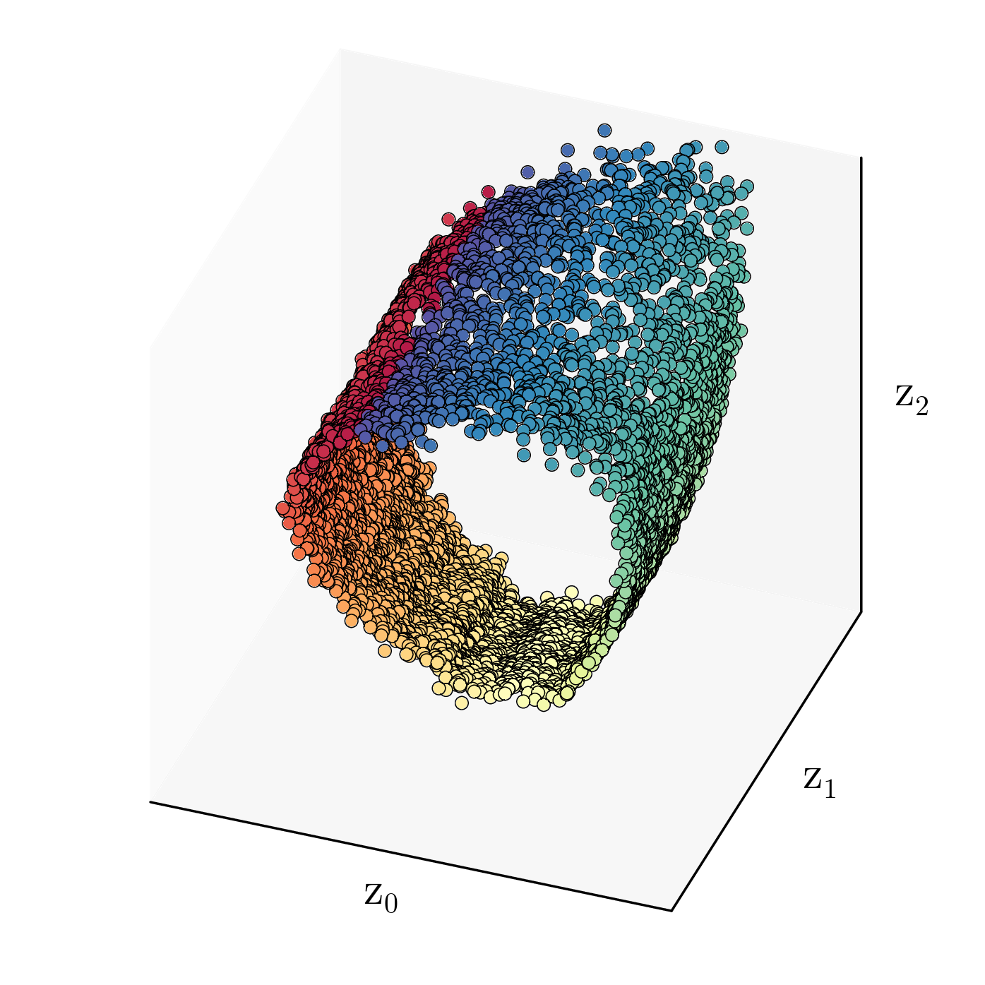
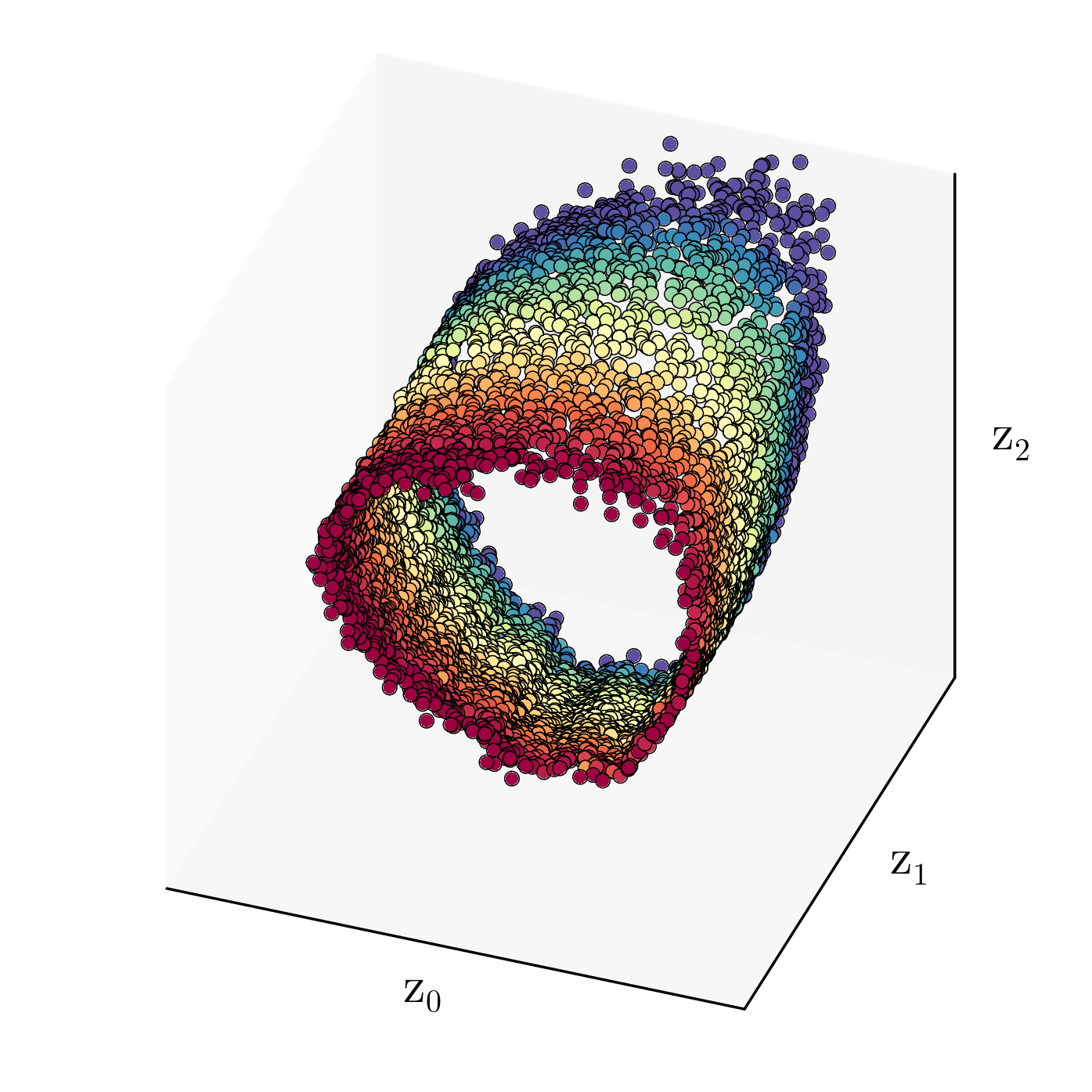
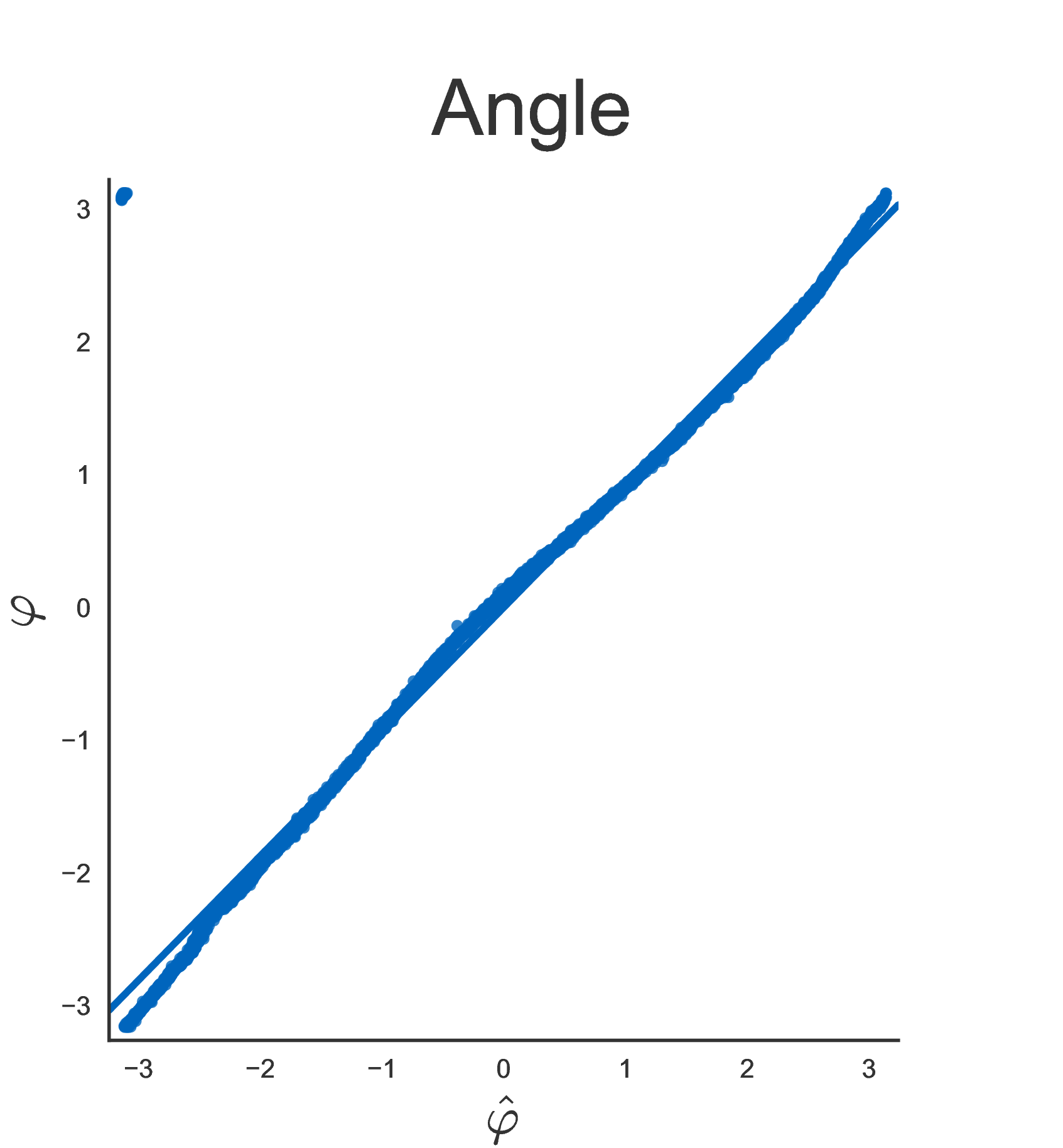
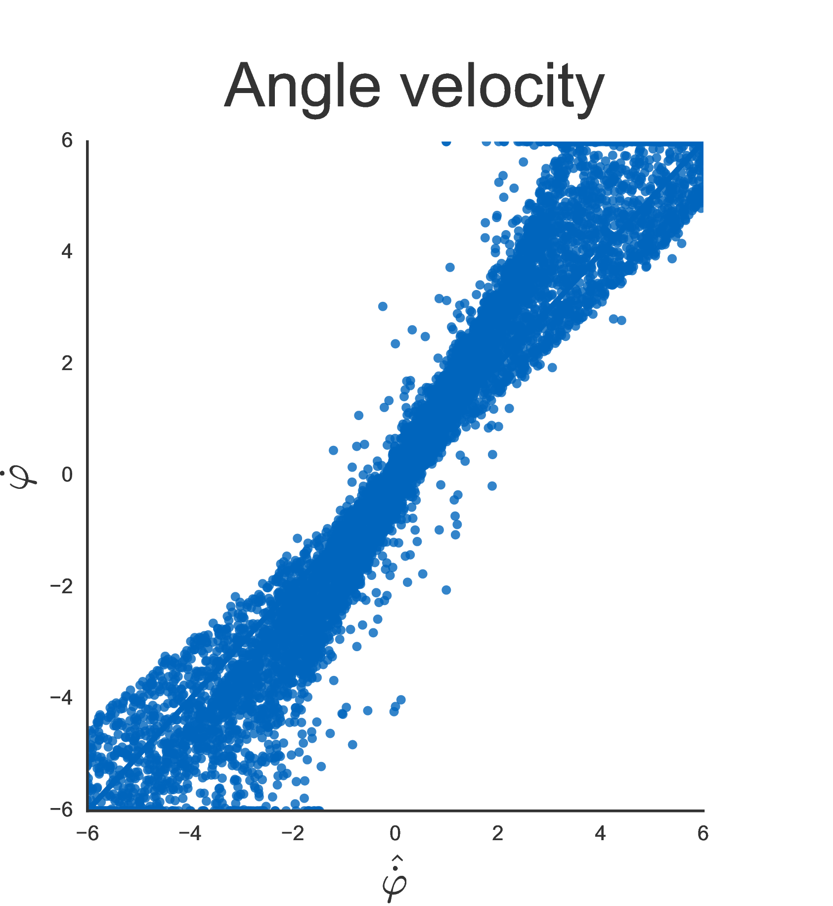
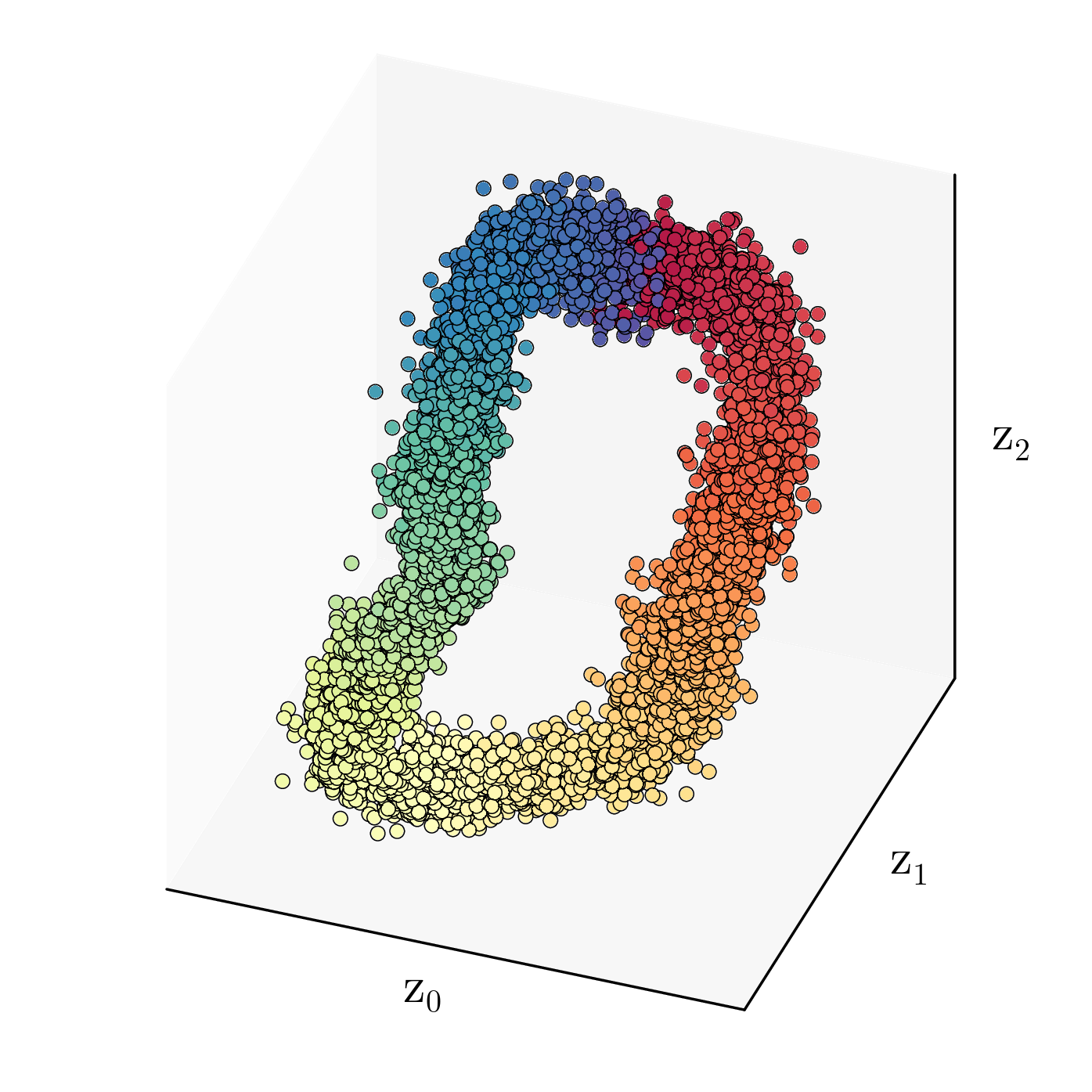
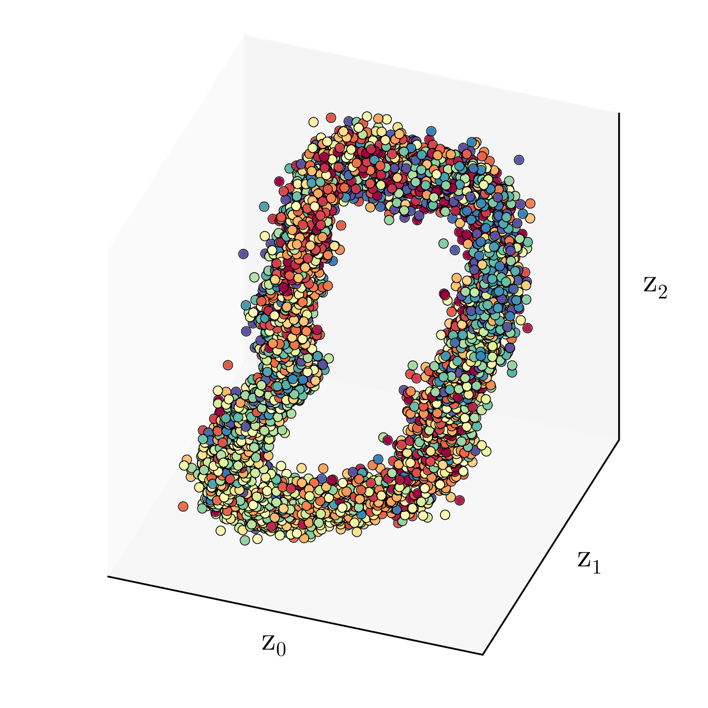
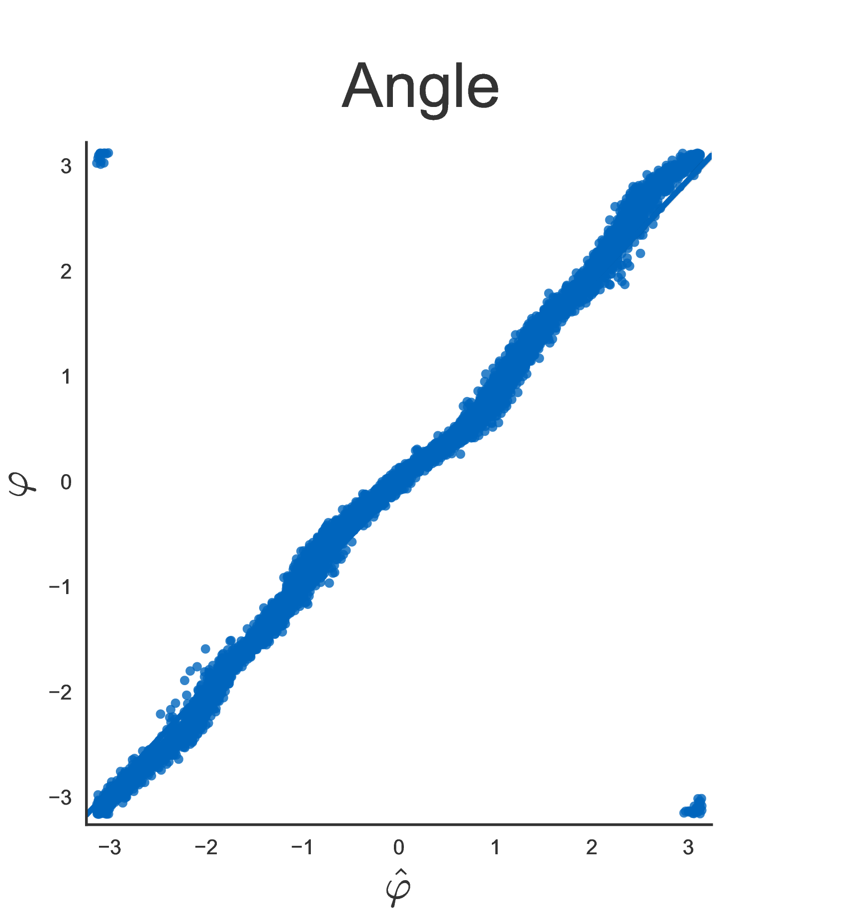
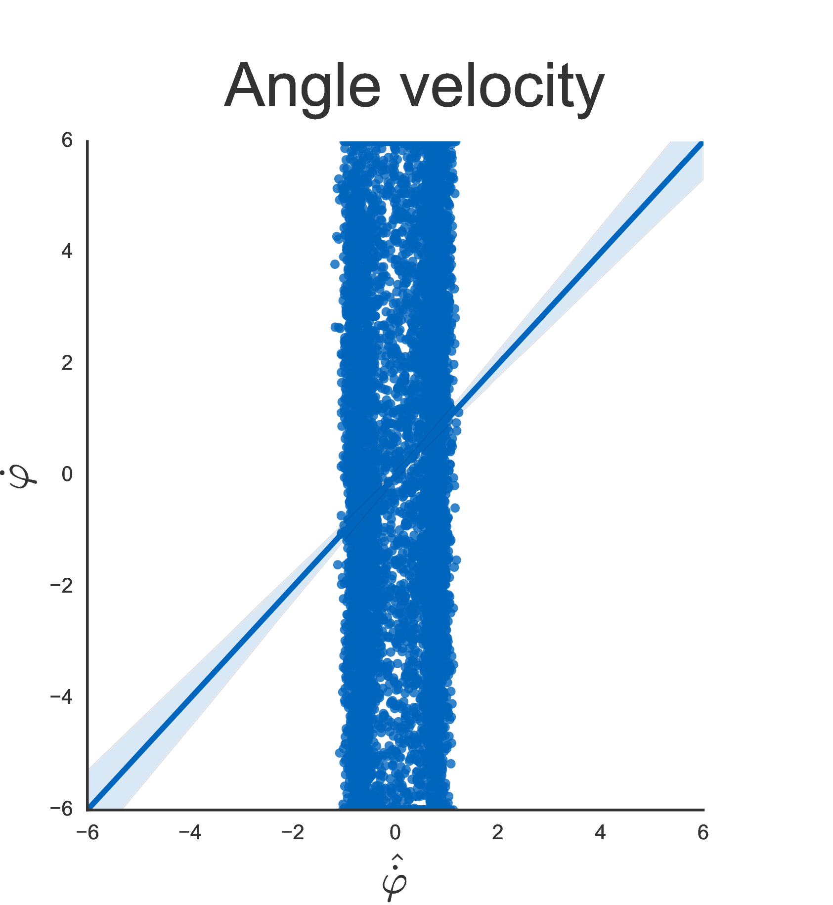
Figure 3 shows the latent spaces for identical input data learned by DVBF-LL and DKF, respectively, colored with the ground truth in the top row. It should be noted that latent samples are shown, not means of posterior distributions. The state-space model was allowed to use three latent dimensions. As we can see in fig. 3(a), DVBF-LL learned a two-dimensional manifold embedding, i.e., it encoded the angle in polar coordinates (thus circumventing the discontinuity of angles modulo $2\pi$). The bottom row shows ordinary least-squares regressions (OLS) underlining the performance: there exists a high correlation between latent states and ground-truth angle and angular velocity for DVBF-LL. On the contrary, fig. 3(b) verifies our prediction that DKF is equally capable of learning the angle, but extracts little to no information on angular velocity.

Table 1: Results for pendulum OLS regressions of all latent states on respective dependent variable.

2cm Dependent
ground truth
variable	DVBF-LL DKF Log-Likelihood $R^{2}$ Log-Likelihood $R^{2}$ $\sin(\varphi)$ 3990.8 0.961 1737.6 0.929 $\cos(\varphi)$ 7231.1 0.982 6614.2 0.979 $\dot{\varphi}$ $-$11139 0.916 $-$20289 0.035

The OLS regression results shown in table 1 validate this observation. Predicting $\sin(\varphi)$ and $\cos(\varphi)$, i.e., polar coordinates of the ground-truth angle $\varphi$, works almost equally well for DVBF-LL and DKF, with DVBF-LL slightly outperforming DKF. For predicting the ground truth velocity $\dot{\varphi}$, DVBF-LL shows remarkable performance. DKF, instead, contains hardly any information, resulting in a very low goodness-of-fit score of $R^{2}=0.035$.

((a))

((b))

((c))

Figure 4: (a) Latent space walk in generative mode. (b) Latent space walk in filtering mode. (c) Ground truth and samples from recognition and generative model. The reconstruction sampling has access to observation sequence and performs filtering. The generative samples only get access to the observations once for creating the initial state while all subsequent samples are predicted from this single initial state. The red bar indicates the length of training sequences. Samples beyond show the generalization capabilities for sequences longer than during training. The complete sequence can be found in the Appendix in fig. 7.

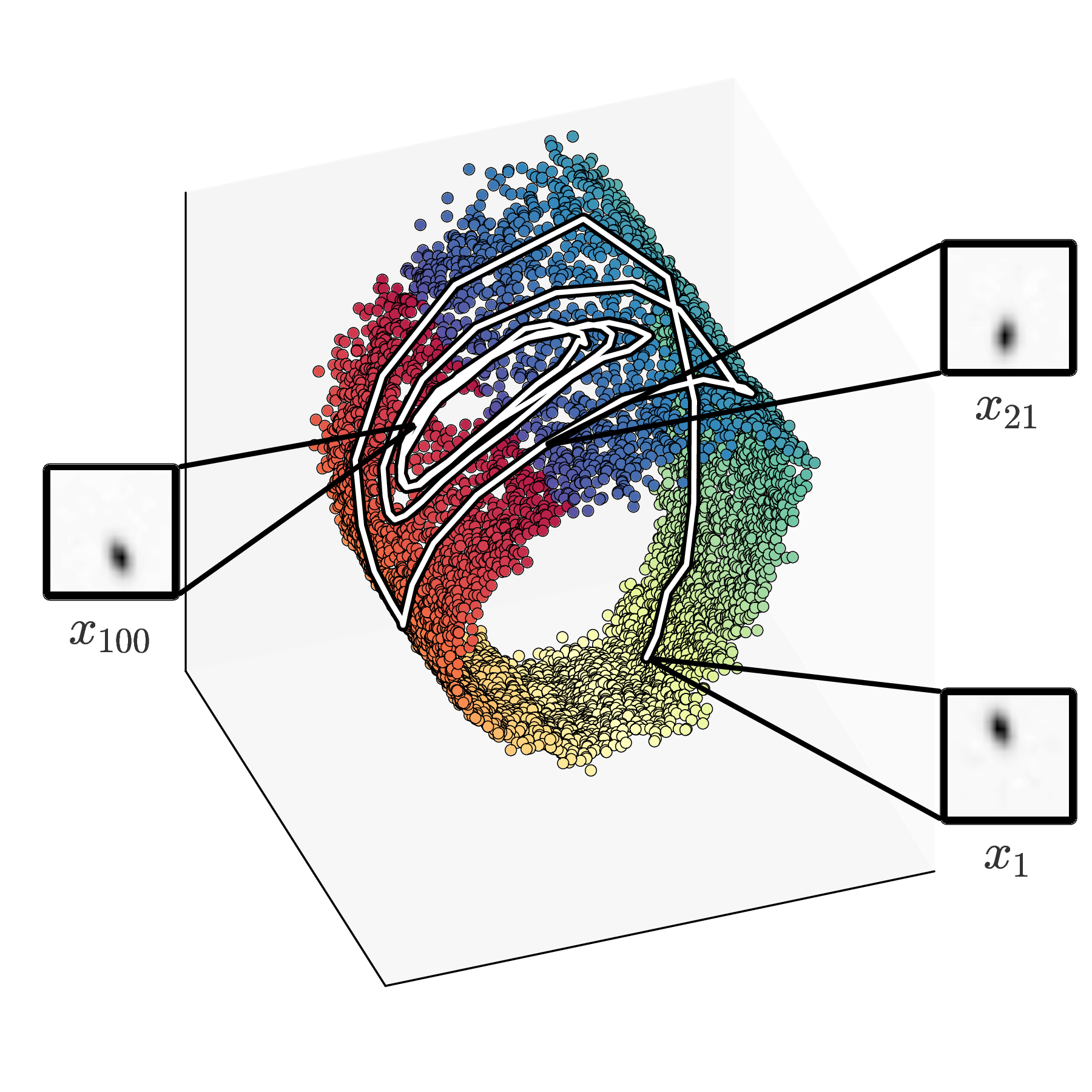
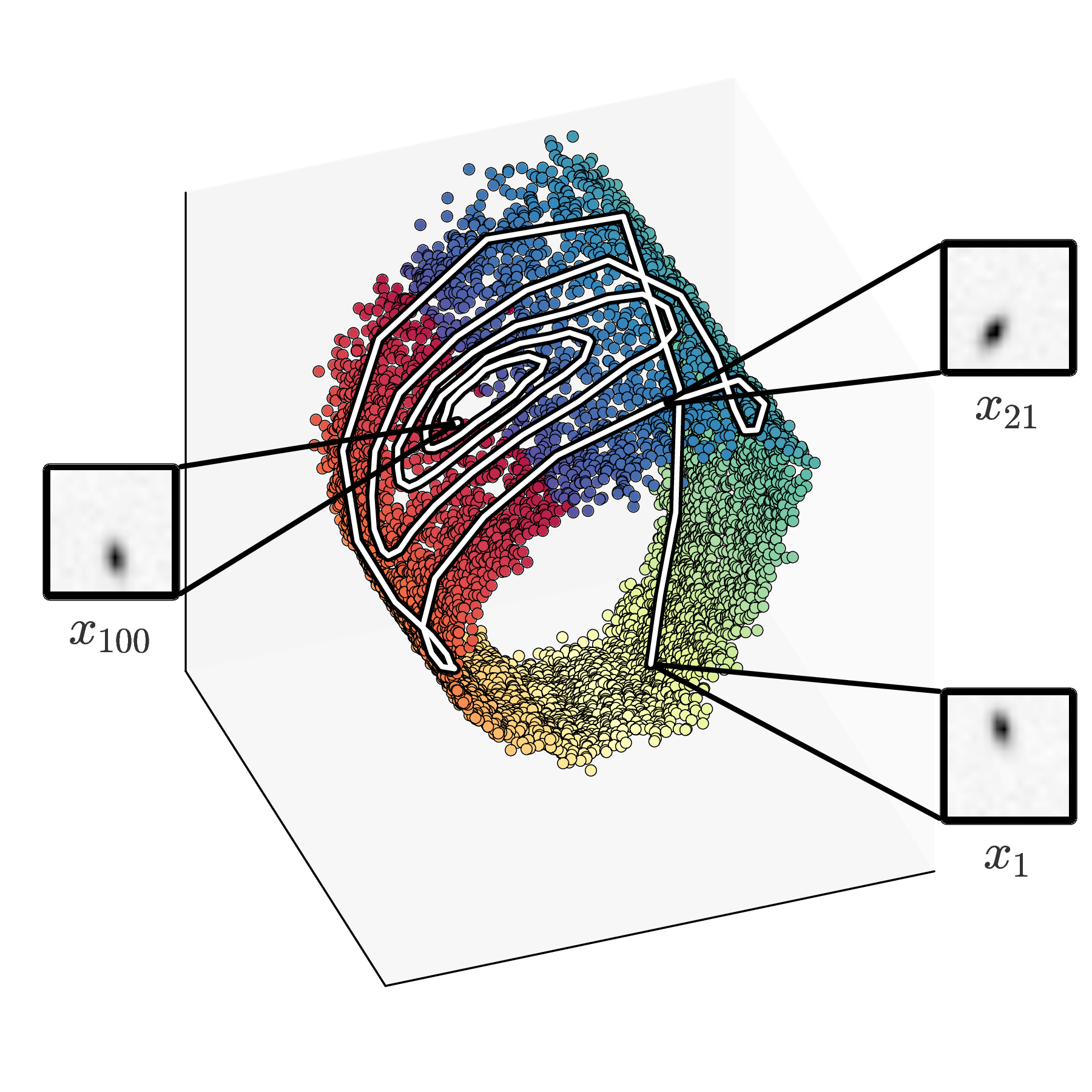
Figure 4 shows that the strong relation between ground truth and latent state is beneficial for generative sampling. All plots show 100 time steps of a pendulum starting from the exact same latent state and not being actuated. The top row plots show a purely generative walk in the latent space on the left, and a walk in latent space that is corrected by filtering observations on the right. We can see that both follow a similar trajectory to an attractor. The generative model is more prone to noise when approaching the attractor.

The bottom plot shows the first 45 steps of the corresponding observations (top row), reconstructions (middle row), and generative samples (without correcting from observations). Interestingly, DVBF works very well even though the sequence is much longer than all training sequences (indicated by the red line).

Table 2: Average test set objective function values for pendulum experiment.

	Lower Bound	$=$	Reconstruction Error	$-$	KL divergence
DVBF-LL	798.56		802.06		3.50
DKF	784.70		788.58		3.88

Table (2) shows values of the lower bound to the marginal data likelihood (for DVBF-LL, this corresponds to eq. 11). We see that DVBF-LL outperforms DKF in terms of compression, but only with a slight margin, which does not reflect the better generative sampling as Theis et al. (2015) argue.

4.2 Bouncing Ball

The bouncing ball experiment features a ball rolling within a bounding box in a plane. The system has a two-dimensional control input, added to the directed velocity of the ball. If the ball hits the wall, it bounces off, so that the true dynamics are highly dependent on the current position and velocity of the ball. The system’s state is four-dimensional, two dimensions each for position and velocity.

((a))

((b))

Figure 5: (a) Two dimensions of 4D bouncing ball latent space. Ground truth x and y coordinates are combined into a regular 3$\times$3 checkerboard coloring. This checkerboard is correctly extracted by the embedding. (b) Remaining two latent dimensions. Same latent samples, colored with ball velocities in x and y direction (left and right image, respectively). The smooth, perpendicular coloring indicates that the ground truth value is stored in the latent dimension.

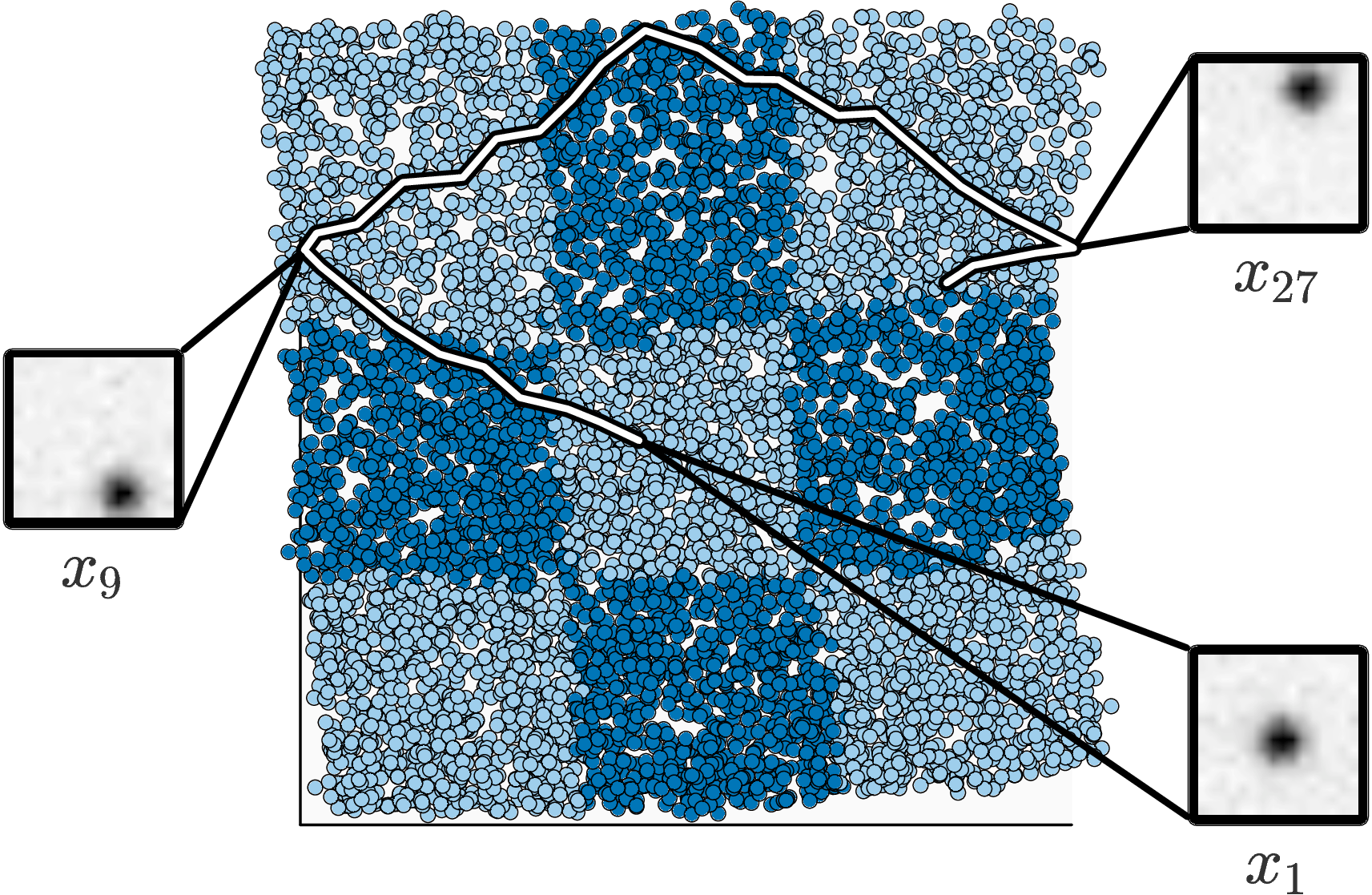
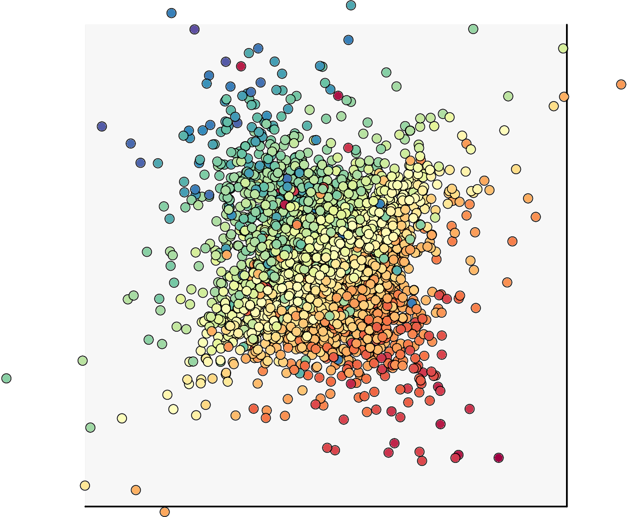
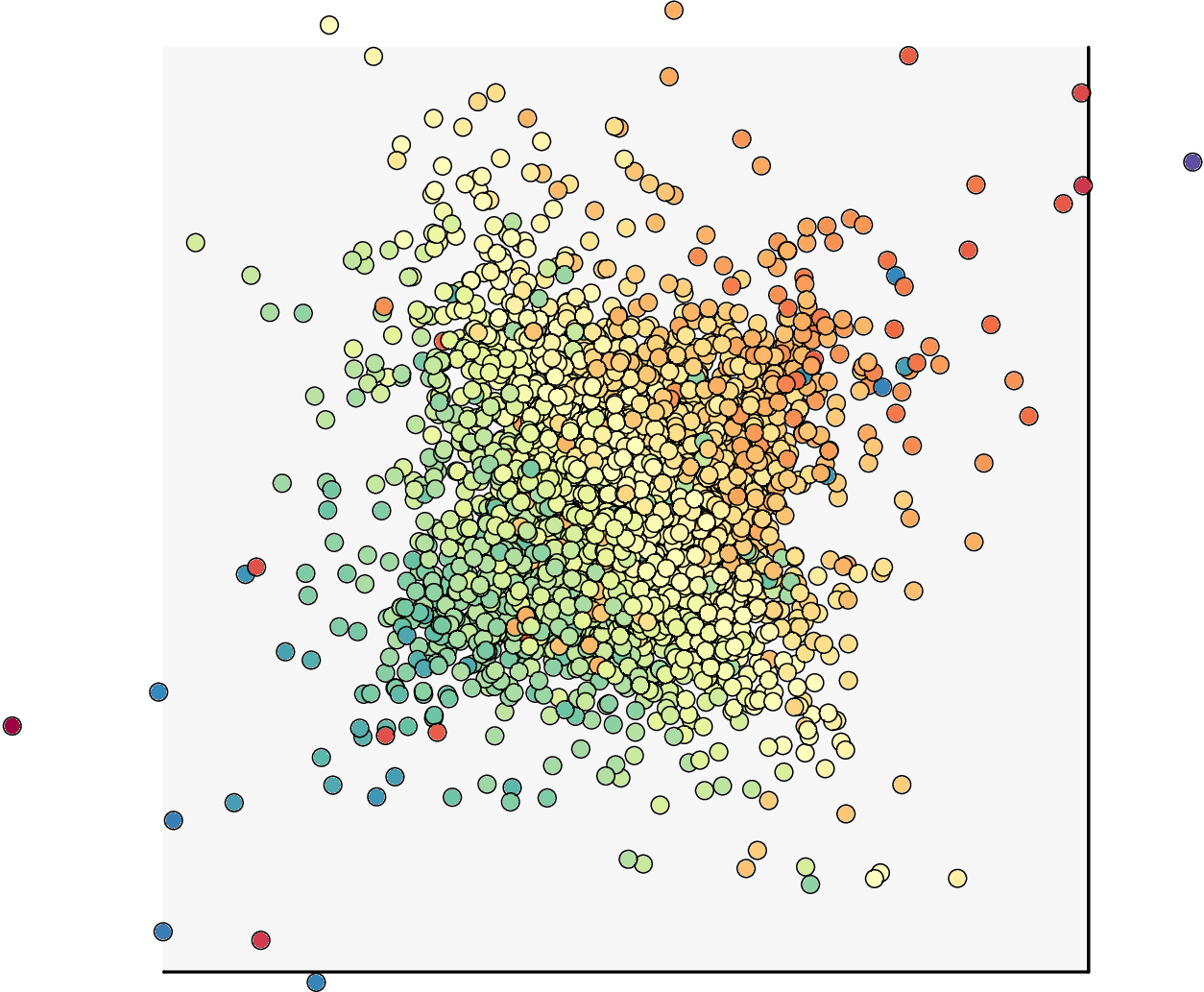
Consequently, we use a DVBF-LL with four latent dimensions. Figure 5 shows that DVBF again captures the entire system dynamics in the latent space. The checkerboard is quite a remarkable result: the ground truth position of the ball lies within the 2D unit square, the bounding box. In order to visualize how ground truth reappears in the learned latent states, we show the warping of the ground truth bounding box into the latent space. To this end, we partitioned (discretized) the ground truth unit square into a regular 3x3 checkerboard with respective coloring. We observed that DVBF learned to extract the 2D position from the 256 pixels, and aligned them in two dimensions of the latent space in strong correspondence to the physical system. The algorithm does the exact same pixel-to-2D inference that a human observer automatically does when looking at the image.

4.3 Two Bouncing Balls

Figure 6: Ground truth (top), reconstructions (middle), generative samples (bottom) from identical initial latent state for the two bouncing balls experiment. Red bar indicates length of training sequences.

Another more complex environment features two balls in a bounding box. We used a 10-dimensional latent space to fully capture the position and velocity information of the balls. Reconstruction and generative samples are shown in fig. 6. Same as in the pendulum example we get a generative model with stable predictions beyond training data sequence length.

5 Conclusion

We have proposed Deep Variational Bayes Filters (DVBF), a new method to learn state space models from raw non-Markovian sequence data. DVBFs perform latent dynamic system identification, and subsequently overcome intractable inference. As DVBFs make use of stochastic gradient variational Bayes they naturally scale to large data sets. In a series of vision-based experiments we demonstrated that latent states can be recovered which identify the underlying physical quantities. The generative model showed stable long-term predictions far beyond the sequence length used during training.

Acknowledgements

Part of this work was conducted at Chair of Robotics and Embedded Systems, Department of Informatics, Technische Universität München, Germany, and supported by the TACMAN project, EC Grant agreement no. 610967, within the FP7 framework programme.

We would like to thank Jost Tobias Springenberg, Adam Kosiorek, Moritz Münst, and anonymous reviewers for valuable input.

Appendix A Supplementary to Lower Bound

A.1 Annealed KL-Divergence

We used the analytical solution of the annealed KL-divergence in eq. 10 for optimization:

$${{\mathbb{E}}_{q_{\phi}}\mathopen{}\mathclose{{}\left[-\ln{q_{\phi}\mathopen{}\mathclose{{}\left(\mathbf{w}_{1:T}\mid\mathbf{x}_{1:T},\mathbf{u}_{1:T}}\right)}+c_{i}\ln p\mathopen{}\mathclose{{}\left(\mathbf{w}_{1:T}}\right)}\right]}=$$

$$c_{i}\frac{1}{2}\ln(2\pi\sigma_{p}^{2})-\frac{1}{2}\ln(2\pi\sigma_{q}^{2})+c_{i}\frac{\sigma_{q}^{2}+(\mu_{q}-\mu_{p})^{2}}{2\sigma_{p}^{2}}-\frac{1}{2}$$

Appendix B Supplementary to Implementation

B.1 Experimental setup

In all our experiments, we use sequences of 15 raw images of the respective system with 16$\times$16 pixels each, i.e., observation space $\mathcal{X}\subset{\mathbb{R}}^{256}$, as well as control inputs of varying dimension and interpretation depending on the experiment. We used training, validation and test sets with 500 sequences each. Control input sequences were drawn randomly (“motor babbling”). Additional details about the implementation can be found in the published code at https://brml.org/projects/dvbf.

B.2 Additional Experiment Plots

Figure 7: Ground truth and samples from recognition and generative model. Complete version of fig. 4 with all missing samples present.

B.3 Implementation details for DVBF in Pendulum Experiment

• Input: 15 timesteps of $16^{2}$ observation dimensions and 1 action dimension

• Latent Space: 3 dimensions

• Observation Network $p(\mathbf{x}_{t}|\mathbf{z}_{t})=\mathcal{N}(\mathbf{x}_{t};\mu(\mathbf{z}_{t}),\sigma)$: 128 ReLU + $16^{2}$ identity output

• Recognition Model: 128 ReLU + 6 identity output

  $$q(\mathbf{w}_{t}|\mathbf{z}_{t},\mathbf{x}_{t+1},\mathbf{u}_{t})=\mathcal{N}(\mathbf{w}_{t};\mu,\sigma),$$

  $$(\mu,\sigma)=f(\mathbf{z}_{t},\mathbf{x}_{t+1},\mathbf{u}_{t})$$

  
  

• Transition Network $\boldsymbol{\alpha}_{t}(\mathbf{z}_{t})$: 16 softmax output

• Initial Network $\mathbf{w}_{1}\sim p(\mathbf{x}_{1:T})$: Fast Dropout BiRNN with: 128 ReLU + 3 identity output

• Initial Transition $\mathbf{z}_{1}(\mathbf{w}_{1})$: 128 ReLU + 3 identity output

• Optimizer: adadelta, 0.1 step rate

• Inverse temperature: $c_{0}=0.01$, updated every 250th gradient update, $T_{A}=10^{5}$ iterations

• Batch-size: 500

B.4 Implementation details for DVBF in Bouncing Ball Experiment

• Input: 15 timesteps of $16^{2}$ observation dimensions and 2 action dimension

• Latent Space: 4 dimensions

• Observation Network $p(\mathbf{x}_{t}|\mathbf{z}_{t})=\mathcal{N}(\mathbf{x}_{t};\mu(\mathbf{z}_{t}),\sigma)$: 128 ReLU + $16^{2}$ identity output

• Recognition Model: 128 ReLU + 8 identity output

  $$q(\mathbf{w}_{t}|\mathbf{z}_{t},\mathbf{x}_{t+1},\mathbf{u}_{t})=\mathcal{N}(\mathbf{w}_{t};\mu,\sigma),$$

  $$(\mu,\sigma)=f(\mathbf{z}_{t},\mathbf{x}_{t+1},\mathbf{u}_{t})$$

  
  

• Transition Network $\boldsymbol{\alpha}_{t}(\mathbf{z}_{t})$: 16 softmax output

• Initial Network $\mathbf{w}_{1}\sim p(\mathbf{x}_{1:T})$: Fast Dropout BiRNN with: 128 ReLU + 4 identity output

• Initial Transition $\mathbf{z}_{1}(\mathbf{w}_{1})$: 128 ReLU + 4 identity output

• Optimizer: adadelta, 0.1 step rate

• Inverse temperature: $c_{0}=0.01$, updated every 250th gradient update, $T_{A}=10^{5}$ iterations

• Batch-size: 500

B.5 Implementation details for DVBF in Two Bouncing Balls Experiment

• Input: 15 timesteps of $20^{2}$ observation dimensions and 2000 samples

• Latent Space: 10 dimensions

• Observation Network $p(\mathbf{x}_{t}|\mathbf{z}_{t})=\mathcal{N}(\mathbf{x}_{t};\mu(\mathbf{z}_{t}),\sigma)$: 128 ReLU + $20^{2}$ sigmoid output

• Recognition Model: 128 ReLU + 20 identity output

  $$q(\mathbf{w}_{t}|\mathbf{z}_{t},\mathbf{x}_{t+1},\mathbf{u}_{t})=\mathcal{N}(\mathbf{w}_{t};\mu,\sigma),$$

  $$(\mu,\sigma)=f(\mathbf{z}_{t},\mathbf{x}_{t+1},\mathbf{u}_{t})$$

  
  

• Transition Network $\boldsymbol{\alpha}_{t}(\mathbf{z}_{t})$: 64 softmax output

• Initial Network $\mathbf{w}_{1}\sim p(\mathbf{x}_{1:T})$: MLP with: 128 ReLU + 10 identity output

• Initial Transition $\mathbf{z}_{1}(\mathbf{w}_{1})$: 128 ReLU + 10 identity output

• Optimizer: adam, 0.001 step rate

• Inverse temperature: $c_{0}=0.01$, updated every gradient update, $T_{A}=2\leavevmode\nobreak\ 10^{5}$ iterations

• Batch-size: 80

B.6 Implementation details for DKF in Pendulum Experiment

• Input: 15 timesteps of $16^{2}$ observation dimensions and 1 action dimension

• Latent Space: 3 dimensions

• Observation Network $p(\mathbf{x}_{t}|\mathbf{z}_{t})=\mathcal{N}(\mathbf{x}_{t};\mu(\mathbf{z}_{t}),\sigma(\mathbf{z}_{t}))$: 128 Sigmoid + 128 Sigmoid + $2\leavevmode\nobreak\ 16^{2}$ identity output

• Recognition Model: Fast Dropout BiRNN 128 Sigmoid + 128 Sigmoid + 3 identity output

• Transition Network $p(\mathbf{z}_{t}|\mathbf{z}_{t-1},\mathbf{u}_{t-1})$: 128 Sigmoid + 128 Sigmoid + 6 output

• Optimizer: adam, 0.001 step rate

• Inverse temperature: $c_{0}=0.01$, updated every 25th gradient update, $T_{A}=2000$ iterations

• Batch-size: 500

References

- Bayer & Osendorfer (2014) Justin Bayer and Christian Osendorfer. Learning stochastic recurrent networks. arXiv preprint arXiv:1411.7610, 2014.
- Blundell et al. (2015) Charles Blundell, Julien Cornebise, Koray Kavukcuoglu, and Daan Wierstra. Weight uncertainty in neural networks. arXiv preprint arXiv:1505.05424, 2015.
- Bottou (2010) Léon Bottou. Large-scale machine learning with stochastic gradient descent. In Proceedings of COMPSTAT’2010, pp. 177–186. Springer, 2010.
- Chung et al. (2015) Junyoung Chung, Kyle Kastner, Laurent Dinh, Kratarth Goel, Aaron C. Courville, and Yoshua Bengio. A recurrent latent variable model for sequential data. CoRR, abs/1506.02216, 2015. URL http://arxiv.org/abs/1506.02216.
- Deisenroth & Rasmussen (2011) Marc Deisenroth and Carl E Rasmussen. Pilco: A model-based and data-efficient approach to policy search. In Proceedings of the 28th International Conference on machine learning (ICML-11), pp. 465–472, 2011.
- Ghahramani & Hinton (1996) Zoubin Ghahramani and Geoffrey E Hinton. Parameter estimation for linear dynamical systems. Technical report, Technical Report CRG-TR-96-2, University of Toronto, Dept. of Computer Science, 1996.
- Ghahramani & Hinton (2000) Zoubin Ghahramani and Geoffrey E Hinton. Variational learning for switching state-space models. Neural computation, 12(4):831–864, 2000.
- Graves (2013) Alex Graves. Generating sequences with recurrent neural networks. arXiv preprint arXiv:1308.0850, 2013.
- Hinton & Van Camp (1993) Geoffrey E Hinton and Drew Van Camp. Keeping the neural networks simple by minimizing the description length of the weights. In Proceedings of the sixth annual conference on Computational learning theory, pp. 5–13. ACM, 1993.
- Honkela et al. (2010) Antti Honkela, Tapani Raiko, Mikael Kuusela, Matti Tornio, and Juha Karhunen. Approximate riemannian conjugate gradient learning for fixed-form variational bayes. Journal of Machine Learning Research, 11(Nov):3235–3268, 2010.
- Johnson et al. (2016) Matthew J Johnson, David Duvenaud, Alexander B Wiltschko, Sandeep R Datta, and Ryan P Adams. Structured VAEs: Composing probabilistic graphical models and variational autoencoders. arXiv preprint arXiv:1603.06277, 2016.
- Julier & Uhlmann (1997) Simon J Julier and Jeffrey K Uhlmann. New extension of the kalman filter to nonlinear systems. In AeroSense’97, pp. 182–193. International Society for Optics and Photonics, 1997.
- Kalman & Bucy (1961) Rudolph E Kalman and Richard S Bucy. New results in linear filtering and prediction theory. Journal of basic engineering, 83(1):95–108, 1961.
- Kingma & Welling (2013) Diederik P Kingma and Max Welling. Auto-encoding variational bayes. arXiv preprint arXiv:1312.6114, 2013.
- Ko & Fox (2011) Jonathan Ko and Dieter Fox. Learning gp-bayesfilters via gaussian process latent variable models. Autonomous Robots, 30(1):3–23, 2011.
- Krishnan et al. (2015) Rahul G Krishnan, Uri Shalit, and David Sontag. Deep Kalman filters. arXiv preprint arXiv:1511.05121, 2015.
- Mandt et al. (2016) Stephan Mandt, James McInerney, Farhan Abrol, Rajesh Ranganath, and David Blei. Variational tempering. In Proceedings of the 19th International Conference on Artificial Intelligence and Statistics, pp. 704–712, 2016.
- McGoff et al. (2015) Kevin McGoff, Sayan Mukherjee, Natesh Pillai, et al. Statistical inference for dynamical systems: A review. Statistics Surveys, 9:209–252, 2015.
- Rezende et al. (2014) Danilo J. Rezende, Shakir Mohamed, and Daan Wierstra. Stochastic backpropagation and approximate inference in deep generative models. In Tony Jebara and Eric P. Xing (eds.), Proceedings of the 31st International Conference on Machine Learning (ICML-14), pp. 1278–1286. JMLR Workshop and Conference Proceedings, 2014. URL http://jmlr.org/proceedings/papers/v32/rezende14.pdf.
- Rezende & Mohamed (2015) Danilo Jimenez Rezende and Shakir Mohamed. Variational inference with normalizing flows. arXiv preprint arXiv:1505.05770, 2015.
- Sutskever & Hinton (2007) Ilya Sutskever and Geoffrey E. Hinton. Learning multilevel distributed representations for high-dimensional sequences. In Marina Meila and Xiaotong Shen (eds.), Proceedings of the Eleventh International Conference on Artificial Intelligence and Statistics (AISTATS-07), volume 2, pp. 548–555. Journal of Machine Learning Research - Proceedings Track, 2007. URL http://jmlr.csail.mit.edu/proceedings/papers/v2/sutskever07a/sutskever07a.pdf.
- Sutton (1996) Leonid Kuvayev Rich Sutton. Model-based reinforcement learning with an approximate, learned model. In Proceedings of the ninth Yale workshop on adaptive and learning systems, pp. 101–105, 1996.
- Theis et al. (2015) Lucas Theis, Aäron van den Oord, and Matthias Bethge. A note on the evaluation of generative models. arXiv preprint arXiv:1511.01844, 2015.
- Valpola & Karhunen (2002) Harri Valpola and Juha Karhunen. An unsupervised ensemble learning method for nonlinear dynamic state-space models. Neural computation, 14(11):2647–2692, 2002.
- Watter et al. (2015) Manuel Watter, Jost Springenberg, Joschka Boedecker, and Martin Riedmiller. Embed to control: A locally linear latent dynamics model for control from raw images. In Advances in Neural Information Processing Systems, pp. 2728–2736, 2015.