Quantifying the accuracy of approximate
diffusions and Markov chains

Abstract.

Markov chains and diffusion processes are indispensable tools in machine learning and statistics that are used for inference, sampling, and modeling. With the growth of large-scale datasets, the computational cost associated with simulating these stochastic processes can be considerable, and many algorithms have been proposed to approximate the underlying Markov chain or diffusion. A fundamental question is how the computational savings trade off against the statistical error incurred due to approximations. This paper develops general results that address this question. We bound the Wasserstein distance between the equilibrium distributions of two diffusions as a function of their mixing rates and the deviation in their drifts. We show that this error bound is tight in simple Gaussian settings. Our general result on continuous diffusions can be discretized to provide insights into the computational–statistical trade-off of Markov chains. As an illustration, we apply our framework to derive finite-sample error bounds of approximate unadjusted Langevin dynamics. We characterize computation-constrained settings where, by using fast-to-compute approximate gradients in the Langevin dynamics, we obtain more accurate samples compared to using the exact gradients. Finally, as an additional application of our approach, we quantify the accuracy of approximate zig-zag sampling. Our theoretical analyses are supported by simulation experiments.

1. Introduction

Markov chains and their continuous-time counterpart, diffusion processes, are ubiquitous in machine learning and statistics, forming a core component of the inference and modeling toolkit. Since faster convergence enables more efficient sampling and inference, a large and fruitful literature has investigated how quickly these stochastic processes converge to equilibrium. However, the tremendous growth of large-scale machine learning datasets – in areas such as social network analysis, vision, natural language processing and bioinformatics – have created new inferential challenges. The large-data setting highlights the need for stochastic processes that are not only accurate (as measured by fast convergence to the target distribution), but also computationally efficient to simulate. These computational considerations have led to substantial research efforts into approximating the underlying stochastic processes with new processes that are more computationally efficient [45, 6, 23].

As an example, consider using Markov chain Monte Carlo (MCMC) to sample from a posterior distribution. In standard algorithms, each step of the Markov chain involves calculating a statistic that depends on all of the observed data (e.g. a likelihood ratio to set the rejection rate in Metropolis-Hastings or a gradient of the log-likelihood as in Langevin dynamics). As data sets grow larger, such calculations increasingly become the computational bottleneck. The need for more scalable sampling algorithms has led to the development of Markov chains which only approximate the desired statistics at each step – for example, by approximating the gradient or sub-sampling the data – and hence are computationally more efficient [45, 14, 30, 28, 5, 6, 36, 23]. The trade-off is that the approximate chain often does not converge to the desired equilibrium distribution, which, in many applications, could be the posterior distribution of some latent parameters given all of the observed data. Therefore, a central question of both theoretical and practical importance is how to quantify the deviation between the equilibrium distribution that the approximate chain converges to and the desired distribution targeted by the original chain. Moreover, we would like to understand, given a fixed computational budget, how to design approximate chains that generate the most accurate samples.

Our contributions. In this paper, we develop general results to quantify the accuracy of approximate diffusions and Markov chains and apply these results to characterize the computational–statistical trade-off in specific algorithms. Our starting point is continuous-time diffusion processes because these are the objects which are discretized to construct many sampling algorithms, such as the unadjusted and Metropolis-adjusted Langevin algorithms [37] and Hamiltonian Monte Carlo [34]. Given two diffusion processes, we bound the deviation in their equilibrium distributions in terms of the deviation in their drifts and the rate at which the diffusion mixes (Theorem 3.1). Moreover, we show that this bound is tight for certain Gaussian target distributions. These characterizations of diffusions are novel and are likely of more general interest beyond the inferential settings we consider. We apply our general results to derive a finite-sample error bound on a specific unadjusted Langevin dynamics algorithm (Theorem 5.1). Under computational constraint, the relevant trade-off here is between computing the exact log-likelihood gradient for few iterations or computing an approximate gradient for more iterations. We characterize settings where the approximate Langevin dynamics produce more accurate samples from the true posterior. We illustrate our analyses with simulation results. In addition, we apply our approach to quantify the accuracy of approximations to the zig-zag process, a recently-developed non-reversible sampling scheme.

Paper outline. We introduce the basics of diffusion processes and other preliminaries in Section 2. Section 3 discusses the main results on bounding the error between an exact and perturbed diffusion. We describe the main ideas behind our analyses in Section 4; all the detailed proofs are deferred to the XXXXXAppendixarxivAppendix. Section 5 applies the main results to derive finite sample error bounds for unadjusted Langevin dynamics and illustrates the computational–statistical trade-off. Section 6 extends our main results to quantify the accuracy of approximate piecewise deterministic Markov processes, including the zig-zag process. Numerical experiments to complement the theory are provided in Section 7. We conclude with a discussion of how our results connect to the relevant literature and suggest directions for further research.

2. Diffusions and preliminaries

Let $\mathcal{X}=\mathbb{R}^{d}$ be the parameter space and let $\pi$ be a probability density over $\mathbb{R}^{d}$ (e.g. it can be the posterior distribution of some latent parameters given data). A Langevin diffusion is characterized by the stochastic differential equation

$$\mathrm{d}X_{t}=\nabla\log\pi(X_{t})\,\mathrm{d}t+\mathchoice{{\hbox{$\displaystyle\sqrt{2\,}$}\lower 0.4pt\hbox{\vrule height=6.44444pt,depth=-5.15558pt}}}{{\hbox{$\textstyle\sqrt{2\,}$}\lower 0.4pt\hbox{\vrule height=6.44444pt,depth=-5.15558pt}}}{{\hbox{$\scriptstyle\sqrt{2\,}$}\lower 0.4pt\hbox{\vrule height=4.51111pt,depth=-3.6089pt}}}{{\hbox{$\scriptscriptstyle\sqrt{2\,}$}\lower 0.4pt\hbox{\vrule height=3.22221pt,depth=-2.57779pt}}}\mathrm{d}W_{t},$$ (2.1)

where $X_{t}\in\mathbb{R}^{d}$ and $W_{t}$ is a standard Brownian motion. The intuition is that $X_{t}$ undergoes a biased random walk in which it is more likely to move in directions that increase the density. Under appropriate regularity conditions, as $t\rightarrow\infty$, the distribution of $X_{t}$ converges to $\pi$. Thus, simulating the Langevin diffusion provides a powerful framework to sample from the target $\pi$. To implement such a simulation, we need to discretize the continuous diffusion into finite-width time steps. For our main results, we focus on analyzing properties of the underlying diffusion processes. This allows us to obtain general results which are independent of any particular discretization scheme.

Beyond Langevin dynamics, more general diffusions can take the form

$$\mathrm{d}X_{t}=b(X_{t})\,\mathrm{d}t+\mathchoice{{\hbox{$\displaystyle\sqrt{2\,}$}\lower 0.4pt\hbox{\vrule height=6.44444pt,depth=-5.15558pt}}}{{\hbox{$\textstyle\sqrt{2\,}$}\lower 0.4pt\hbox{\vrule height=6.44444pt,depth=-5.15558pt}}}{{\hbox{$\scriptstyle\sqrt{2\,}$}\lower 0.4pt\hbox{\vrule height=4.51111pt,depth=-3.6089pt}}}{{\hbox{$\scriptscriptstyle\sqrt{2\,}$}\lower 0.4pt\hbox{\vrule height=3.22221pt,depth=-2.57779pt}}}\mathrm{d}W_{t},$$ (2.2)

where $b:\mathbb{R}^{d}\rightarrow\mathbb{R}^{d}$ is the drift and is not necessarily the gradient of some log-density. Furthermore, we can analyze other continuous-time Markov processes such as piecewise deterministic Markov processes (PDMPs). For example, Hamiltonian Monte Carlo [34] can be viewed as approximating a PDMP and the zig-zag process is a recently-developed non-reversible PDMP designed for large Bayesian inference (see Section 6).

In many large-data settings, computing the drift $b(X_{t})$ in Eq. 2.2 can be expensive; for example, computing $b(X_{t})=\nabla\log\pi(X_{t})$ requires using all of the data and may involve evaluating a complex function such as a differential equation solver. Many recent algorithms have been proposed where we replace $b$ with an approximation $\tilde{b}$. Such an approximation changes the underlying diffusion process to

$$\mathrm{d}\tilde{X}_{t}=\tilde{b}(\tilde{X}_{t})\,\mathrm{d}t+\mathchoice{{\hbox{$\displaystyle\sqrt{2\,}$}\lower 0.4pt\hbox{\vrule height=6.44444pt,depth=-5.15558pt}}}{{\hbox{$\textstyle\sqrt{2\,}$}\lower 0.4pt\hbox{\vrule height=6.44444pt,depth=-5.15558pt}}}{{\hbox{$\scriptstyle\sqrt{2\,}$}\lower 0.4pt\hbox{\vrule height=4.51111pt,depth=-3.6089pt}}}{{\hbox{$\scriptscriptstyle\sqrt{2\,}$}\lower 0.4pt\hbox{\vrule height=3.22221pt,depth=-2.57779pt}}}\mathrm{d}\tilde{W}_{t},$$ (2.3)

where $\tilde{W}_{t}$ is a standard Brownian motion. In order to understand the quality of different approximations, we need to quantify how the equilibrium distribution of Eq. 2.2 differs from the equilibrium distribution of Eq. 2.3. We use the standard Wasserstein metric to measure this distance.

Definition.

The Wasserstein distance between distributions $\pi$ and $\tilde{\pi}$ is

$$d_{\mathcal{W}}(\pi,\tilde{\pi})=\sup_{\phi\in C_{L}(\mathbb{R}^{d})}|E_{\pi}[\phi]-E_{\tilde{\pi}}[\phi]|,$$ (2.4)

where $C_{L}(\mathbb{R}^{d})$ is the set of continuous functions $\phi:\mathbb{R}^{d}\to\mathbb{R}$ with Lipschitz constant $\|\phi\|_{L}\leq 1$.

The distance between $\pi$ and $\tilde{\pi}$ should depend on how good the drift approximation is, which can be quantified by $\|b-\tilde{b}\|_{2}$. It is also natural for the distance to depend on how quickly the original diffusion with drift $b$ mixes, since the faster it mixes, the less time there is for the error to accumulate. Geometric contractivity is a useful property which quantifies fast-mixing diffusions. For each $x\in\mathbb{R}^{d}$, let $\mu_{x,t}$ denote the law of $X_{t}\,|\,X_{0}=x$.

Assumption 2.A (Geometric contractivity).

There exist constants $C>0$ and $0<\rho<1$ such that for all $x,x^{\prime}\in\mathbb{R}^{d}$,

$$d_{\mathcal{W}}(\mu_{x,t},\mu_{x^{\prime},t})\leq C\|x-x^{\prime}\|_{2}\rho^{t}.$$ (2.5)

Geometric contractivity holds in many natural settings. Recall that a twice continuously-differentiable function $\phi$ is $k$-strongly concave if for all $x,x^{\prime}\in\mathbb{R}^{d}$

$$(\nabla\phi(x)-\nabla\phi(x^{\prime}))\cdot(x-x^{\prime})\leq-k\|x-x^{\prime}\|_{2}^{2}.$$ (2.6)

When $b=\nabla\log\pi$ and $\log\pi$ is $k$-strongly concave, the diffusion is exponentially ergodic with $C=1$ and $\rho=e^{-k}$ (this can be shown using standard coupling arguments [11]). In fact, exponential contractivity also follows if Eq. 2.6 is satisfied when $x$ and $x^{\prime}$ are far apart and $\log\pi$ has “bounded convexity” when $x$ and $x^{\prime}$ are close together [20]. Alternatively, Hairer et al. [25] provides a Lyapunov function-based approach to proving exponential contractivity.

To ensure that the diffusion and the approximate diffusion are well-behaved, we impose some standard regularity properties.

Assumption 2.B (Regularity conditions).

Let $\pi$ and $\tilde{\pi}$ denote the stationary distributions of the diffusions in Eq. 2.2 and Eq. 2.3, respectively.

1. The target density satisfies $\pi\in C^{2}(\mathbb{R}^{d},\mathbb{R})$ and $\int x^{2}\pi(\mathrm{d}x)<\infty$. The drift satisfies $b\in C^{1}(\mathbb{R}^{d},\mathbb{R}^{d})$ and $\|b\|_{L}<\infty$.

2. The approximate drift satisfies $\tilde{b}\in C^{1}(\mathbb{R}^{d},\mathbb{R}^{d})$ and $\|\tilde{b}\|_{L}<\infty$.

3. If a function $\phi\in C(\mathbb{R}^{d},\mathbb{R})$ is $\pi$-integrable then it is $\tilde{\pi}$-integrable.

Here $C^{k}(\mathbb{R}^{m},\mathbb{R}^{n})$ denotes the set of $k$-times continuously differentiable functions from $\mathbb{R}^{m}$ to $\mathbb{R}^{n}$ and $C(\mathbb{R}^{m},\mathbb{R}^{n})$ is the set of all Lebesgue-measurable function from $\mathbb{R}^{m}$ to $\mathbb{R}^{n}$. The only notable regularity condition is (3). In the XXXXXAppendixarxivAppendix, we discuss how to verify it and why it can safely be treated as a mild technical condition.

3. Main results

We can now state our main result, which quantifies the deviation in the equilibrium distributions of the two diffusions in terms of the mixing rate and the difference between the diffusions’ drifts.

Theorem 3.1 (Error induced by approximate drift).

Let $\pi$ and $\tilde{\pi}$ denote the invariant distributions of the diffusions in Eq. 2.2 and Eq. 2.3, respectively. If the diffusion Eq. 2.2 is exponentially ergodic with parameters $C$ and $\rho$, the regularity conditions of Assumption 2.B hold, and $\|b-\tilde{b}\|_{2}\leq\epsilon$, then

$$d_{\mathcal{W}}(\pi,\tilde{\pi})\leq\frac{C\epsilon}{\log(1/\rho)}.$$ (3.1)

Remark 3.2 (Coherency of the error bound).

To check that the error bound of Eq. 3.1 has coherent dependence on its parameters, consider the following thought experiment. Suppose we change the time scale of the diffusion from $t$ to $s=at$ for some $a>0$. We are simply speeding up or slowing down the diffusion process depending on whether $a>1$ or $a<1$. Changing the time scale does not affect the equilibrium distribution and hence $d_{\mathcal{W}}(\pi,\tilde{\pi})$ remains unchanged. After time $s$ has passed, the exponential contraction is $\rho^{at}$ and hence the effective contraction constant is $\rho^{a}$ instead of $\rho$. Moreover, the drift at each location is also scaled by $a$ and hence the drift error is $\epsilon a$. The scaling $a$ thus cancels out in the error bound, which is desirable since the error should be independent of how we set the time scale.

Remark 3.3 (Tightness of the error bound).

We can choose $b$ and $\tilde{b}$ such that the bound in Eq. 3.1 is an equality, thus showing that, under the assumptions considered, Theorem 3.1 cannot be improved. Let $\pi(x)=\mathscr{N}(x;\mu,\sigma^{2}I)$ be the Gaussian density with mean $\mu\in\mathbb{R}^{d}$ and covariance matrix $\sigma^{2}I$ and let $\tilde{\pi}(x)=\mathscr{N}(x;\tilde{\mu},\sigma^{2}I)$. The Wasserstein distance between two Gaussians with the same covariance is the distance between their means, so $d_{\mathcal{W}}(\pi,\tilde{\pi})=\|\mu-\tilde{\mu}\|_{2}$. Consider the corresponding diffusions where $b=\nabla\log\pi$ and $\tilde{b}=\nabla\log\tilde{\pi}$. We have that for any $x\in\mathbb{R}^{d}$, $\|b(x)-\tilde{b}(x)\|_{2}=\sigma^{-2}\|\mu-\tilde{\mu}\|_{2}=:\epsilon$. Furthermore, the Hessian is $H[\log\pi]=-\sigma^{-2}I$, which implies that $b$ is $\sigma^{-2}$-strongly concave. Therefore, per the discussion in Section 2, exponential contractivity holds with $C=1$ and $\rho=e^{-\sigma^{-2}}$. We thus conclude that

$$\frac{C\epsilon}{\log(1/\rho)}=\frac{\sigma^{-2}\|\mu-\tilde{\mu}\|_{2}}{\sigma^{-2}}=\|\mu-\tilde{\mu}\|_{2}=d_{\mathcal{W}}(\pi,\tilde{\pi}).$$ (3.2)

and hence the bound of Theorem 3.1 is tight in this setting.

Theorem 3.1 assumes that the approximate drift is a deterministic function and that the error in the drift is uniformly bounded. We can generalize the results of Theorem 3.1 to allow for the approximate diffusion to use stochastic drift with non-uniform drift error. We will see that only the expected magnitude of the drift bias affects the final error bound. Let $\tilde{b}(\tilde{X}_{t},\tilde{Y}_{t})$ denote the approximate drift, which is now a function of both the current location $\tilde{X}_{t}$ and an independent diffusion $\tilde{Y}_{t}\in\mathbb{R}^{\ell}$:

$$\mathrm{d}\tilde{X}_{t}=(\tilde{b}(\tilde{X}_{t},\tilde{Y}_{t}))\,\mathrm{d}t+\mathchoice{{\hbox{$\displaystyle\sqrt{2\,}$}\lower 0.4pt\hbox{\vrule height=6.44444pt,depth=-5.15558pt}}}{{\hbox{$\textstyle\sqrt{2\,}$}\lower 0.4pt\hbox{\vrule height=6.44444pt,depth=-5.15558pt}}}{{\hbox{$\scriptstyle\sqrt{2\,}$}\lower 0.4pt\hbox{\vrule height=4.51111pt,depth=-3.6089pt}}}{{\hbox{$\scriptscriptstyle\sqrt{2\,}$}\lower 0.4pt\hbox{\vrule height=3.22221pt,depth=-2.57779pt}}}\mathrm{d}\tilde{W}_{t}^{X}$$ (3.3)

$$\mathrm{d}\tilde{Y}_{t}=b_{aux}(\tilde{Y}_{t})\,\mathrm{d}t+\Sigma\,\mathrm{d}\tilde{W}^{Y}_{t},$$ (3.4)

where $\Sigma$ is an $\ell\times\ell$ matrix and the notation $\tilde{W}_{t}^{X}$ and $\tilde{W}_{t}^{Y}$ highlights that the Brownian motions in $\tilde{X}_{t}$ and $\tilde{Y}_{t}$ are independent. Let $\tilde{\pi}_{Z}$ denote the stationary distribution of $\tilde{Z}_{t}\triangleq(\tilde{X}_{t},\tilde{Y}_{t})$. For measure $\mu$ and function $f$, we write $\mu(f)\triangleq\int f(x)\mu(\mathrm{d}x)$ to reduce clutter. We can now state a generalization of Theorem 3.1.

Theorem 3.4 (Error induced by stochastic approximate drift).

Let $\pi$ and $\tilde{\pi}$ denote the invariant distributions of the diffusions in Eqs. 2.2 and 3.3, respectively. Assume that there exists a measurable function $\epsilon\in C(\mathbb{R}^{d},\mathbb{R}_{+})$ such that for $(\tilde{X},\tilde{Y})\sim\tilde{\pi}_{Z}$ and for all $x\in\mathbb{R}^{d}$,

$$\|b(x)-\mathbb{E}[\tilde{b}(\tilde{X},\tilde{Y})\,|\,\tilde{X}=x]\|_{2}\leq\epsilon(x).$$ (3.5)

If the diffusion Eq. 2.2 is exponentially ergodic and the regularity conditions of Assumption 2.B hold, then

$$d_{\mathcal{W}}(\pi,\tilde{\pi})\leq\frac{C\,\tilde{\pi}(\epsilon)}{\log(1/\rho)}.$$ (3.6)

Whereas the bound of Theorem 3.1 is proportional to the deterministic drift error $\epsilon$, the bound for the diffusion with a stochastic approximate drift is proportional to the expected drift error bound $\tilde{\pi}(\epsilon)$. The bound of Theorem 3.4 thus takes into account how the drift error varies with the location of the drift. Our results match the asymptotic behavior for stochastic gradient Langevin dynamics documented in Teh et al. [42]: in the limit of the step size going to zero, they show that the stochastic gradient has no effect on the equilibrium distribution.

Example.

Suppose $\tilde{Y}_{t}$ is an Ornstein–Uhlenbeck process with $\ell=d$, the dimensionality of $\tilde{X}_{t}$. That is, for some $\alpha,v>0$, $\mathrm{d}\tilde{Y}_{t}=-\alpha\tilde{Y}_{t}\mathrm{d}t+\mathchoice{{\hbox{$\displaystyle\sqrt{2v\,}$}\lower 0.4pt\hbox{\vrule height=6.44444pt,depth=-5.15558pt}}}{{\hbox{$\textstyle\sqrt{2v\,}$}\lower 0.4pt\hbox{\vrule height=6.44444pt,depth=-5.15558pt}}}{{\hbox{$\scriptstyle\sqrt{2v\,}$}\lower 0.4pt\hbox{\vrule height=4.51111pt,depth=-3.6089pt}}}{{\hbox{$\scriptscriptstyle\sqrt{2v\,}$}\lower 0.4pt\hbox{\vrule height=3.22221pt,depth=-2.57779pt}}}\mathrm{d}\tilde{W}_{t}^{Y}$. Then the equilibrium distribution of $\tilde{Y}_{t}$ is that of a Gaussian with covariance $\sigma^{2}I$, where $\sigma^{2}\triangleq v/\alpha$. Let $\tilde{b}(x,y)=b(x)+y$, so $\mathbb{E}[\tilde{b}(\tilde{X},\tilde{Y})\,|\,\tilde{X}=x]=b(x)$ and hence $d_{\mathcal{W}}(\pi,\tilde{\pi})=0$.

While exponential contractivity is natural and applies in many settings, it is useful to have bounds on the Wasserstein distance of approximations when the diffusion process mixes more slowly. We can prove the analogous guarantee of Theorem 3.1 when a weaker, polynomial contractivity condition is satisfied.

Assumption 3.C (Polynomial contractivity).

There exist constants $C>0$, $\alpha>1$, and $\beta>0$ such that for all $x,x^{\prime}\in\mathbb{R}^{d}$,

$$d_{\mathcal{W}}(\mu_{x,t},\mu_{x^{\prime},t})\leq C\|x-x^{\prime}\|_{2}(t+\beta)^{-\alpha}.$$ (3.7)

The parameters $\alpha$ and $\beta$ determines how quickly the diffusion converges to equilibrium. Polynomial contractivity can be certified using, for example, the techniques from Butkovsky [13] (see also the references therein).

Theorem 3.5 (Error induced by approximate drift, polynomial contractivity).

Let $\pi$ and $\tilde{\pi}$ denote the invariant distributions of the diffusions in Eq. 2.2 and Eq. 2.3, respectively. If the diffusion Eq. 2.2 is polynomially ergodic with parameters $C$, $\alpha$, and $\beta$, the regularity conditions of Assumption 2.B hold, and $\|b-\tilde{b}\|_{2}\leq\epsilon$, then

$$d_{\mathcal{W}}(\pi,\tilde{\pi})\leq\frac{C\epsilon}{(\alpha-1)\beta^{\alpha-1}}.$$ (3.8)

Remark 3.6 (Coherency of the error bound).

The error bound of Eq. 3.8 has a coherent dependence on its parameters, just like Eq. 3.1. If we change the time scale of the diffusion from $t$ to $s=at$ for some $a>0$, the polynomial contractivity constants $C,\alpha$, and $\beta$ become, respectively, $C/a^{\alpha},\alpha$, and $\beta/a$. Making these substitutions and replacing $\epsilon$ by $\epsilon a$, one can check that the scaling $a$ cancels out in the error bound, so the error is independent of how we set the time scale.

4. Overview of analysis techniques

We use Stein’s method [40, 4, 38] to bound the Wasserstein distance between $\pi$ and $\tilde{\pi}$ as a function of a bound on $\|b-\tilde{b}\|_{2}$ and the mixing time of $\pi$. We describe the analysis ideas for the setting when $\|b-\tilde{b}\|_{2}<\epsilon$ (Theorem 3.1); the analysis with stochastic drift (Theorem 3.4) or assuming polynomial contractivity (Theorem 3.5) is similar. All of the details are in the XXXXXAppendixarxivAppendix.

For a diffusion $(X_{t})_{t\geq 0}$ with drift $b$, the corresponding infinitesimal generator satisfies

$$\mathcal{A}_{b}\phi(x) =b(x)\cdot\nabla\phi(x)+\Delta\phi(x)$$ (4.1)

for any function $\phi$ that is twice continuously differentiable and vanishing at infinity. See, e.g., Ethier and Kurtz [21] for an introduction to infinitesimal generators. Under quite general conditions, the invariant measure $\pi$ and the generator $\mathcal{A}_{b}$ satisfy

$$\pi(\mathcal{A}_{b}\phi)=0.$$ (4.2)

For any measure $\nu$ on $\mathbb{R}^{d}$ and set of test functions $\mathcal{F}\subseteq C^{2}(\mathbb{R}^{d},\mathbb{R})$, we can define the Stein discrepancy as:

$$\mathcal{S}(\nu,\mathcal{A}_{b},\mathcal{F}) \triangleq\sup_{\phi\in\mathcal{F}}|\pi(\mathcal{A}_{b}\phi)-\nu(\mathcal{A}_{b}\phi)|=\sup_{\phi\in\mathcal{F}}|\nu(\mathcal{A}_{b}\phi)|.$$ (4.3)

The Stein discrepancy quantifies the difference between $\nu$ and $\pi$ in terms of the maximum difference in the expected value of a function (belonging to the transformed test class $\{\mathcal{A}_{b}\phi\,|\,\phi\in\mathcal{F}\}$) under these two distributions. We can analyze the Stein discrepancy between $\pi$ and $\tilde{\pi}$ as follows. Consider a test set $\mathcal{F}$ such that $\|\nabla\phi\|_{2}\leq 1$ for all $\phi\in\mathcal{F}$, which is equivalent to having $\|\phi\|_{L}\leq 1$. We have that

$$\mathcal{S}(\tilde{\pi},\mathcal{A}_{b},\mathcal{F}) =\sup_{\phi\in\mathcal{F}}|\tilde{\pi}(\mathcal{A}_{b}\phi)|=\sup_{\phi\in\mathcal{F}}|\tilde{\pi}(\mathcal{A}_{b}\phi-\mathcal{A}_{\tilde{b}}\phi)|$$ (4.4)

$$=\sup_{\phi\in\mathcal{F}}|\tilde{\pi}(\nabla\phi\cdot b-\nabla\phi\cdot\tilde{b})|$$ (4.5)

$$\leq\sup_{\phi\in\mathcal{F}}|\tilde{\pi}(\|\nabla\phi\|_{2}\|b-\tilde{b}\|_{2})|\leq\epsilon,$$ (4.6)

where we have used the definition of Stein discrepancy, that $\tilde{\pi}(\mathcal{A}_{\tilde{b}}\phi)=0$, the definition of the generator, the Cauchy-Schwartz inequality, that $\|\nabla\phi\|_{2}\leq 1$, and the assumption $\|b-\tilde{b}\|_{2}\leq\epsilon$. It remains to show that the Wasserstein distance satisfies $d_{\mathcal{W}}(\pi,\tilde{\pi})\leq C_{\pi}\mathcal{S}(\tilde{\pi},\mathcal{A}_{b},\mathcal{F})$ for some constant $C_{\pi}$ that may depend on $\pi$. This would then allow us to conclude that $d_{\mathcal{W}}(\pi,\tilde{\pi})\leq C_{\pi}\epsilon$. To obtain $C_{\pi}$, for each 1-Lipschitz function $h$, we construct the solution $u_{h}$ to the differential equation

$$h-\pi(h)=\mathcal{A}_{g}u$$ (4.7)

and show that $\|\nabla u_{h}\|_{2}\leq C_{\pi}\|\nabla h\|_{2}$. XXXXX4.7

5. Application: computational–statistical trade-offs

As an application of our results we analyze the behavior of the unadjusted Langevin Monte Carlo algorithm (ULA) [37] when approximate gradients of the log-likelihood are used. ULA uses a discretization of the continuous-time Langevin diffusion to approximately sample from the invariant distribution of the diffusion. We prove conditions under which we can obtain more accurate samples by using an approximate drift derived from a Taylor expansion of the exact drift.

For the diffusion $(X_{t})_{t\geq 0}$ driven by drift $b$ as defined in Eq. 2.2 and a non-increasing sequence of step sizes $(\gamma_{i})_{i\geq 1}$, the associated ULA Markov chain is arxiv

$$X^{\prime}_{i+1} =X^{\prime}_{i}+\gamma_{i+1}\,b(X^{\prime}_{i})+\mathchoice{{\hbox{$\displaystyle\sqrt{2\gamma_{i+1}\,}$}\lower 0.4pt\hbox{\vrule height=6.44444pt,depth=-5.15558pt}}}{{\hbox{$\textstyle\sqrt{2\gamma_{i+1}\,}$}\lower 0.4pt\hbox{\vrule height=6.44444pt,depth=-5.15558pt}}}{{\hbox{$\scriptstyle\sqrt{2\gamma_{i+1}\,}$}\lower 0.4pt\hbox{\vrule height=4.51111pt,depth=-3.6089pt}}}{{\hbox{$\scriptscriptstyle\sqrt{2\gamma_{i+1}\,}$}\lower 0.4pt\hbox{\vrule height=3.22221pt,depth=-2.57779pt}}}\xi_{i+1}, \xi_{i+1}\overset{\textrm{\tiny{i.i.d.}}}{\sim}\mathscr{N}(0,1).$$ (5.1)

XXXXX

$$X^{\prime}_{i+1} =X^{\prime}_{i}+\gamma_{i+1}\,b(X^{\prime}_{i})+\mathchoice{{\hbox{$\displaystyle\sqrt{2\gamma_{i+1}\,}$}\lower 0.4pt\hbox{\vrule height=6.44444pt,depth=-5.15558pt}}}{{\hbox{$\textstyle\sqrt{2\gamma_{i+1}\,}$}\lower 0.4pt\hbox{\vrule height=6.44444pt,depth=-5.15558pt}}}{{\hbox{$\scriptstyle\sqrt{2\gamma_{i+1}\,}$}\lower 0.4pt\hbox{\vrule height=4.51111pt,depth=-3.6089pt}}}{{\hbox{$\scriptscriptstyle\sqrt{2\gamma_{i+1}\,}$}\lower 0.4pt\hbox{\vrule height=3.22221pt,depth=-2.57779pt}}}\xi_{i+1},$$ (5.2)

where $\xi_{i+1}\overset{\textrm{\tiny{i.i.d.}}}{\sim}\mathscr{N}(0,1)$. Recently, substantial progress has been made in understanding the approximation accuracy of ULA [16, 12, 18]. These analyses show, as a function of the discretization step size $\gamma_{i}$, how quickly the distribution of $X^{\prime}_{i}$ converges to the desired target distribution.

In many big data settings, however, computing $b(X^{\prime}_{i})$ exactly at every step is computationally expensive. Given a fixed computational budget, one option is to compute $b(X^{\prime}_{i})$ precisely and run the discretized diffusion for a small number of steps to generate samples. Alternatively, we could replace $b(X^{\prime}_{i})$ with an approximate drift $\tilde{b}(X^{\prime}_{i})$ which is cheaper to compute and run the discretized approximate diffusion for a larger number of steps to generate samples. While approximating the drift can introduce error, running for more steps can compensate by sampling from a better mixed chain. Thus, our objective is to compare the ULA chain using an exact drift initialized at some point $x^{\star}\in\mathbb{R}^{d}$ to a ULA chain using an approximate drift initialized at the same point. We denote the exact and approximate drift chains by $X^{\prime}_{x^{\star},i}$ and $\tilde{X}^{\prime}_{x^{\star},i}$, respectively, and denote laws of these chains by $\mu^{\star}_{i}$ and $\tilde{\mu}^{\star}_{i}$.

For concreteness, we analyze generalized linear models with unnormalized log-densities of the form

$$\mathcal{L}(x)\triangleq\log\pi_{0}(x)+\sum_{i=1}^{N}\phi_{i}(x\cdot y_{i}),$$ (5.3)

where $y_{1},\dots,y_{N}\in\mathbb{R}^{d}$ is the data and $x$ is the parameter. In this setting the drift is $b(x)=\nabla\mathcal{L}(x)$. We take $x^{\star}=\operatornamewithlimits{arg\,max}_{x}\mathcal{L}(x)$ and approximate the drift with a Taylor expansion around $x^{\star}$: arxiv

$$\tilde{b}(x)\triangleq(H\log\pi_{0})(x^{\star})(x-x^{\star})+\sum_{i=1}^{N}\phi_{i}^{\prime\prime}(x^{\star}\cdot y_{i})y_{i}y_{i}^{\top}(x-x^{\star}),$$ (5.4)

XXXXX

$$\begin{split}\tilde{b}(x)&\triangleq(H\log\pi_{0})(x^{\star})(x-x^{\star})\\ &\phantom{\triangleq~{}}+\sum_{i=1}^{N}\phi_{i}^{\prime\prime}(x^{\star}\cdot y_{i})y_{i}y_{i}^{\top}(x-x^{\star}),\end{split}$$

where $H$ is the Hessian operator. The quadratic approximation of Section 5 basically corresponds to taking a Laplace approximation of the log-likelihood. In practice, higher-order Taylor truncation or other approximations can be used, and our analysis can be extended to quantify the trade-offs in those cases as well. Here we focus on the second-order approximation as a simple illustration of the computational–statistical trade-off.

In order for the Taylor approximation to be well-behaved, we require the prior $\pi_{0}$ and link functions $\phi_{i}$ to satisfying some regularity conditions, which are usually easy to check in practice.

Assumption 5.D (Concavity, smoothness, and asymptotic behavior of data).

1. The function $\log\pi_{0}\in C^{3}(\mathbb{R}^{d},\mathbb{R})$ is strongly concave, $\|\nabla\log\pi_{0}\|_{L}<\infty$, and $\|H[\partial_{j}\log\pi_{0}]\|_{2}<\infty$ for $j=1,\dots,d$, where $\|\cdot\|_{2}$ denotes the matrix spectral norm.

2. For $i=1,\dots,N$, the function $\phi_{i}\in C^{3}(\mathbb{R},\mathbb{R})$ is strongly concave, $\|\phi_{i}^{\prime}\|_{L}<\infty$, and $\|\phi_{i}^{\prime\prime\prime}\|_{\infty}<\infty$.

3. The data satisfies $\|\sum_{i=1}^{N}y_{i}y_{i}^{\top}\|_{2}=\Theta(N)$.

We measure computational cost by the number of $d$-dimensional inner products performed. Running ULA with the original drift $b$ for $T$ steps costs $TN$ because each step needs to compute $x\cdot y_{i}$ for each of the $N$ $y_{i}$’s. Running ULA with the Taylor approximation $\tilde{b}$, we need to compute $\sum_{i=1}^{N}\phi_{i}^{\prime\prime}(x^{\star}\cdot y_{i})y_{i}y_{i}^{\top}$ once up front, which costs $Nd$, and then for each step we just multiply this $d$-by-$d$ matrix with $x-x^{\star}$, which costs $d$. So the total cost of running approximate ULA for $\tilde{T}$ steps is $(\tilde{T}+N)d$.

Theorem 5.1 (Computational–statistical trade-off for ULA).

Set the step size $\gamma_{i}=\gamma_{1}i^{-\alpha}$ for fixed $\alpha\in(0,1)$ and suppose the ULA of Eq. 5.2 is run for $T>d$ steps. If Assumption 5.D holds and $\tilde{T}$ is chosen such that the computational cost of the second-order approximate ULA using drift Section 5 equals that of the exact ULA, then $\gamma_{1}$ may be chosen such that arxiv

$$d_{\mathcal{W}}^{2}(\mu^{\star}_{T},\pi)=\tilde{O}\left(\frac{d}{TN}\right)\qquad\text{and}\qquad d_{\mathcal{W}}^{2}(\tilde{\mu}^{\star}_{\tilde{T}},\pi)=\tilde{O}\left(\frac{d^{2}}{N^{2}T}+\frac{d^{3}}{N^{2}}\right).$$ (5.5)

XXXXX

$$d_{\mathcal{W}}^{2}(\mu^{\star}_{T},\pi) =\tilde{O}\left(\frac{d}{TN}\right)$$ (5.6)

and

$$d_{\mathcal{W}}^{2}(\tilde{\mu}^{\star}_{\tilde{T}},\pi) =\tilde{O}\left(\frac{d^{2}}{N^{2}T}+\frac{d^{3}}{N^{2}}\right).$$ (5.7)

The ULA procedure of Eq. 5.2 has Wasserstein error decreasing like $1/N$ for data size $N$. Because approximate ULA can be run for more steps at the same computational cost, its error decreases as $1/N^{2}$. Thus, for large $N$ and fixed $T$ and $d$, approximate ULA with drift $\tilde{b}$ achieves more accurate sampling than ULA with $b$. A conceptual benefit of our results is that we can cleanly decompose the final error into the discretization error and the equilibrium bias due to approximate drift. Our theorems in Section 3 quantifies the equilibrium bias, and we can apply existing techniques to bound the discretization error.

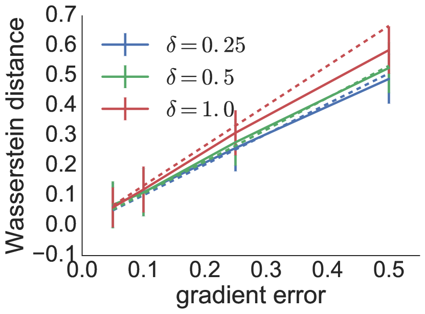
(a)

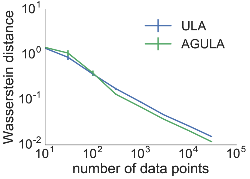
(b)

Figure 1. (a) Gradient error $\epsilon$ versus the Wasserstein distance between $\pi_{\delta}$ and $\tilde{\pi}_{\delta,\epsilon}$, the stationary distribution of the diffusion with approximate drift $\tilde{b}_{\delta,\epsilon}(x)=\nabla\log\pi_{\delta}(x)+\epsilon$. The solid lines are the simulation results and the dotted lines are the theoretical upper bounds obtained from Theorem 3.1. The simulation results closely match the theoretical bounds and show linear growth in $\epsilon$, as predicted by the theory. Due to Monte Carlo error the simulation estimates sometimes slightly exceed the theoretical bounds. (b) The $y$-axis measures the Wasserstein distance between the true posterior distribution and the finite-time distribution of the exact gradient ULA (ULA) and the approximate gradient ULA (AGULA). Except for when the number of data points $N<100$, AGULA shows superior performance, in agreement with the analysis of Theorem 5.1. For all experiments the Wasserstein distance was estimated 10 times, each time using 1,000 samples from each distribution.

XXXXX XXXXX

6. Extension: piecewise deterministic Markov processes

We next demonstrate the generality of our techniques by providing a perturbation analysis of piecewise deterministic Markov processes (PDMPs), which are continuous-time processes that are deterministic except at random jump times. Originating with the work of Davis [17], there is now a rich literature on the ergodic and convergence properties of PDMPs [15, 7, 22, 2, 32]. They have been used to model a range of phenomena including communication networks, neuronal activity, and biologic population models (see [2] and references therein). Recently, PDMPs have also been used to design novel MCMC inference schemes. zig-zag processes (ZZPs) [10, 8, 9] are a class of PDMPs that are particularly promising for inference. ZZPs can be simulated exactly (making Metropolis-Hastings corrections unnecessary) and are non-reversible, which can potentially lead to more efficient sampling [31, 33].

Our techniques can be readily applied to analyze the accuracy of approximate PDMPs. For concreteness we demonstrate the results for ZZPs in detail and defer the general treatment of PDMPs, which includes an idealized version of Hamiltonian Monte Carlo, to the XXXXXAppendixarxivAppendix. The ZZP is defined on the space $E=\mathbb{R}^{d}\times\mathcal{B}$, where $\mathcal{B}\triangleq\{-1,+1\}^{d}$. Densities on $\mathcal{B}$ are with respect to the counting measure.

Informally, the behavior of a ZZP can be described as follows. The trajectory is $X_{t}$ and its velocity is $\Theta_{t}$, so $\frac{d}{dt}X_{t}=\Theta_{t}$. At random times, a single coordinate of $\Theta_{t}$ flips signs. In between these flips, the velocity is a constant and the trajectory is a straight line (hence the name “zig-zag”). The rate at which $\Theta_{t}$ flips a coordinate is time inhomogeneous. The $i$-th component of $\Theta$ switches at rate $\lambda_{i}(X_{t},\Theta_{t})$. By choosing the switching rates appropriately, the ZZP can be made to sample from the desired distribution. More precisely, the ZZP $(X_{t},\Theta_{t})_{t\geq 0}$ is determined by the switching rate $\lambda\in C^{0}(E,\mathbb{R}_{+}^{d})$ and has generator

$$\mathcal{A}_{\lambda}\phi(x,\theta)=\theta\cdot\nabla_{x}\phi(x,\theta)+\lambda(x,\theta)\cdot\nabla_{\theta}\phi(x,\theta)$$ (6.1)

for any sufficiently regular $\phi:E\to\mathbb{R}$. Here $\nabla_{x}\phi$ denotes the gradient of $\phi$ with respect to $x$ and $\nabla_{\theta}\phi$ is the discrete differential operator. Let $(a)^{+}\triangleq\max(0,a)$ denote the positive part of $a\in\mathbb{R}$ and $\partial_{i}\phi\triangleq\frac{\partial\phi}{\partial x_{i}}$. The following result shows how to construct a ZZP with invariant distribution $\pi$.

Theorem 6.1 (Bierkens et al. [10, Theorem 2.2, Proposition 2.3]).

Suppose $\log\pi\in C^{1}(\mathbb{R}^{d})$ and $\gamma\in C^{0}(E,\mathbb{R}^{d}_{+})$ satisfies $\gamma_{i}(x,\theta)=\gamma_{i}(x,R_{i}\theta)$. Let

$$\lambda_{i}(x,\theta)=(-\theta_{i}\partial_{i}\log\pi(x))^{+}+\gamma_{i}(x,\theta).$$ (6.2)

Then the Markov process with generator $\mathcal{A}_{\lambda}$ has invariant distribution $\pi_{E}(\mathrm{d}x,\theta)=2^{-d}\pi(\mathrm{d}x)$.

Analogously to the approximate diffusion setting, we compare $(X_{t},\Theta_{t})_{t\geq 0}$ to an approximating ZZP $(\tilde{X}_{t},\tilde{\Theta}_{t})_{t\geq 0}$ with switching rate $\tilde{\lambda}\in C^{0}(E,\mathbb{R}_{+}^{d})$. For example, if $\tilde{\pi}$ is an approximating density, the approximate switching rate could be chosen as

$$\tilde{\lambda}_{i}(x,\theta)=(-\theta_{i}\partial_{i}\log\tilde{\pi}(x))^{+}+\gamma_{i}(x,\theta).$$ (6.3)

To relate the errors in the switching rates to the Wasserstein distance in the final distributions, we use the same strategy as before: apply Stein’s method to the ZZP generator in Eq. 6.1. We rely on ergodicity and regularity conditions that are analogous to those for diffusions. We write $(X_{x,\theta,t},\Theta_{x,\theta,t})$ to denote the version of the ZZP satisfying $(X_{x,\theta,0},\Theta_{x,\theta,0})=(x,\theta)$ and denote its law by $\mu_{x,\theta,t}$.

Assumption 6.E (ZZP polynomial ergodicity).

There exist constants $C>0$, $\alpha>1$, and $\beta>0$ such that for all $x\in\mathbb{R}^{d}$, $\theta\in\mathcal{B}$, and $i\in[d]$,

$$d_{\mathcal{W}}(\mu_{x,\theta,t},\mu_{x,R_{i}\theta,t}) \leq C(t+\beta)^{-\alpha}.$$ (6.4)

The ZZP polynomial ergodicity condition is looser than that used for diffusions. Indeed, we only need a quantitative bound on the ergodicity constant when the chains are started with the same $x$ value. Together with the fact that $\mathcal{B}$ is compact, this simplifies verification of the condition, which can be done using well-developed coupling techniques from the PDMP literature [7, 22, 2, 32] as well as more general Lyapunov function-based approaches [25].

Our main result of this section bounds the error in the invariant distributions due to errors in the ZZP switching rates. It is more natural to measure the error between $\lambda$ and $\tilde{\lambda}$ in terms of the $\ell^{1}$ norm.

Theorem 6.2 (ZZP error induced by approximate switching rate).

Assume the ZZP with switching rate $\lambda$ (respectively $\tilde{\lambda}$) has invariant distribution $\pi$ (resp. $\tilde{\pi}$). Also assume that $\int_{E}x^{2}\pi(\mathrm{d}x,\mathrm{d}\theta)<\infty$ and if a function $\phi\in C(E,\mathbb{R})$ is $\pi$-integrable then it is $\tilde{\pi}$-integrable. If the ZZP with switching rate $\lambda$ is polynomially ergodic with constants $C$, $\alpha$, and $\beta$ and $\|\lambda-\tilde{\lambda}\|_{1}\leq\epsilon$, then

$$d_{\mathcal{W}}(\pi,\tilde{\pi})\leq\frac{C\epsilon}{(\alpha-1)\beta^{\alpha-1}}.$$ (6.5)

Remark 6.3.

If the approximate switching rate takes the form of Eq. 6.3, then $\|\nabla\log\pi-\nabla\log\tilde{\pi}\|_{1}\leq\epsilon$ implies $\|\lambda-\tilde{\lambda}\|_{1}\leq\epsilon$.

XXXXX

7. Experiments

XXXXX We used numerical experiments to investigate whether our bounds capture the true behavior of approximate diffusions and their discretizations.

Approximate Diffusions. For our theoretical results to be a useful guide in practice, we would like the Wasserstein bounds to be reasonably tight and have the correct scaling in the problem parameters (e.g., in $\|b-\tilde{b}\|_{2}$). To test our main result concerning the error induced from using an approximate drift (Theorem 3.1), we consider mixtures of two Gaussian densities of the form

$$\pi_{\delta}(x)=\frac{1}{2(2\pi)^{d/2}}\left(e^{-\|x-\delta/2\|_{2}^{2}/2}+e^{-\|x+\delta/2\|_{2}^{2}/2}\right),$$ (7.1)

where $\delta\in\mathbb{R}^{d}$ parameterizes the difference between the means of the Gaussians. If $\|\delta\|_{2}<2$, then $\pi_{\delta}$ is $(1-\|\delta\|_{2}/4)$-strongly log-concave; if $\|\delta\|_{2}=2$, then $\pi_{\delta}$ is log-concave; and if $\|\delta\|_{2}>2$, then $\pi_{\delta}$ is not log-concave, but is log-concave in the tails. Thus, for all choices of $\delta$, the diffusion with drift $b_{\delta}(x)\triangleq\nabla\log\pi_{\delta}(x)$ is exponentially ergodic. Importantly, this class of Gaussian mixtures allows us to investigate a range of practical regimes, from strongly unimodal to highly multi-modal distributions. For $d=1$ and a variety of choices of $\delta$, we generated 1,000 samples from the target distribution $\pi_{\delta}$ (which is the stationary distribution of a diffusion with drift $b_{\delta}(x)$) and from $\tilde{\pi}_{\delta,\epsilon}$ (which is the stationary distribution of the approximate diffusion with drift $\tilde{b}_{\delta,\epsilon}(x)\triangleq b_{\delta}(x)+\epsilon$) for $\epsilon=0.05,0.1,0.25,0.5$. We then calculated the Wasserstein distance between the empirical distribution of the target and the empirical distribution of each approximation. Fig. 1(a) shows the empirical Wasserstein distance (solid lines) for $\delta=0.25,0.5,1.0$ along with the corresponding theoretical bounds from Theorem 3.1 (dotted lines). The two are in close agreement. We also investigated larger distances for $\delta=1.0,2.0,3.0$. Here the exponential contractivity constants that can be derived from Eberle [20] are rather loose. Importantly, however, for all values of $\delta$ considered, the Wasserstein distance grows linearly in $\epsilon$, as predicted by our theory. Results for $d>1$ show similar linear behavior in $\epsilon$, though we omit the plots.

Computational–statistical trade-off. We illustrate the computational–statistical trade-off of Theorem 5.1 in the case of logistic regression. This corresponds to $\phi_{i}(t)=\phi_{lr}(t)\triangleq-\log(1+e^{-t})$. We generate data $y_{1},y_{2},\dots$ according to the following process:

$$z_{i} \sim{\sf{Bern}}(.5), \zeta_{i} \sim\mathscr{N}(\mu_{z_{i}},I), y_{i} =(2z_{i}-1)\zeta_{i},$$ (7.2)

where $\mu_{0}=(0,0,1,1)$ and $\mu_{1}=(1,1,0,0)$. We restrict the domain $\mathcal{X}$ to a ball of radius 3, $\mathcal{X}=\{x\in\mathbb{R}^{4}\,|\,\|x\|_{2}\leq 3\}$, and add a projection step to the ULA algorithm [12], replacing $Z^{\prime}_{i}$ with $\operatornamewithlimits{arg\,min}_{z\in\mathcal{X}}\|Z^{\prime}_{i}-z\|_{2}$. While Theorem 5.1 assumes $\mathcal{X}=\mathbb{R}^{4}$, the numerical results here on the bounded domain still illustrate our key point: for the same computational budget, computing fast approximate gradients and running the ULA chain for longer can produce a better sampler. Fig. 1(b) shows that except for very small $N$, the approximate gradient ULA (AGULA), which uses the approximation in Section 5, produces better performance than exact gradient ULA (ULA) with the same budget. For each data-set size ($N$), the true posterior distribution was estimated by running an adaptive Metropolis-Hastings (MH) sampler for 100,000 iterations. ULA and AGULA were each run 1,000 times to empirically estimate the approximate posteriors. We then calculated the Wasserstein distance between the ULA and AGULA empirical distributions and the empirical distribution obtained from the MH sampler.

XXXXX

8. Discussion

XXXXX Related Work. Recent theoretical work on scalable MCMC algorithms has yielded numerous insights into the regimes in which such methods produce computational gains [35, 39, 1, 26, 27]. Many of these works focused on approximate Metropolis-Hastings algorithms, rather than gradient-based MCMC. Moreover, the results in these papers are for discrete chains, whereas our results also apply to continuous diffusions as well as other continuous-time Markov processes such as the zig-zag process. Perhaps the closest to our work is that of Rudolf and Schweizer [39] and Gorham et al. [24]. The former studies general perturbations of Markov chains and includes an application to stochastic Langevin dynamics. They also rely on a Wasserstein contraction condition, like our Assumption 2.A, in conjunction with a Lyapunov condition on the perturbed chain. However, our more specialized analysis is particularly transparent and leads to tighter bounds in terms of the contraction constant $\rho$: the bound of Rudolf and Schweizer [39] is proportional to $(1-\rho)^{-1}$ whereas our bound is proportional to $-(\log\rho)^{-1}$. Another advantage of our approach is that our results are more straightforward to apply since we do not need to directly analyze the Lyapunov potential and the perturbation ratios as in Rudolf and Schweizer [39]. Our techniques also apply to the weaker polynomial contraction setting. Gorham et al. [24] have results of similar flavor to ours and also rely on Stein’s method, but their assumptions and target use cases differ from ours. Our results in Section 5, which apply when ULA is used with a deterministic approximation to the drift, complement the work of Teh et al. [42] and Vollmer et al. [43], which provides (non-)asymptotic analysis when the drift is approximated stochastically at each iteration.

Conclusion. We have established general results on the accuracy of diffusions with approximate drifts. As an application, we show how this framework can quantify the computational–statistical trade-off in approximate gradient ULA. The example in Section 7 illustrates how the log-concavity constant can be estimated in practice and how theory provides reasonably precise error bounds. We expect our general framework to have many further applications. In particular, an interesting direction is to extend our framework to analyze the trade-offs in subsampling Hamiltonian Monte Carlo algorithms and stochastic Langevin dynamics.

Acknowledgments

Thanks to Natesh Pillai for helpful discussions and to Trevor Campbell for feedback on an earlier draft. Thanks to Ari Pakman for pointing out some typos and to Nick Whiteley for noticing Theorem 5.1 was missing a necessary assumption. JHH is supported by the U.S. Government under FA9550-11-C-0028 and awarded by the DoD, Air Force Office of Scientific Research, National Defense Science and Engineering Graduate (NDSEG) Fellowship, 32 CFR 168a.

Appendix A Exponential contractivity

A natural generalization of the strong concavity case is to assume that $\log\pi$ is strongly concave for $x$ and $x^{\prime}$ far apart and that $\log\pi$ has “bounded convexity” when $x$ and $x^{\prime}$ are close together. It turns out that in such cases Assumption 2.A still holds. More formally, the following assumption can be used even when the drift is not a gradient. For $f:\mathcal{X}\to\mathbb{R}^{d}$ and $r>0$, let

$$\kappa(r)\triangleq\inf\left\{-2\frac{(f(x)-f(x^{\prime}))\cdot(x-x^{\prime})}{r^{2}}:x,x^{\prime}\in\mathcal{X},\|x-x^{\prime}\|_{2}=r\right\}.$$ (A.1)

Define the constant $R_{0}=\inf\{R\geq 0:\kappa(r)\geq 0~{}\forall r\geq R\}$.

Assumption A.6 (Strongly log-concave tails).

For the function $f\in C^{1}(\mathcal{X},\mathbb{R}^{d})$, there exist constants $R,\ell\in[0,\infty)$ and $k\in(0,\infty)$ such that

$$\begin{aligned} \kappa(r)\geq-\ell\text{ for all }r\leq R\text{ and }\kappa(r)\geq k\text{ for all }r>R.\end{aligned}$$ (A.2)

Furthermore, $\kappa(r)$ is continuous and $\int_{0}^{1}r\kappa(r)^{-}\mathrm{d}r<\infty$.

Theorem A.1 (Eberle [20], Wang [44]).

If Assumption A.6 holds for $f=b$ then Assumption 2.A holds for

$$C =\exp\left(\frac{1}{4}\int_{0}^{R_{0}}r\kappa(r)\mathrm{d}s\right)$$ (A.3)

$$\frac{1}{\log(1/\rho)} \leq\begin{cases}\frac{3e}{2}\max(R^{2},8k^{-1})&\text{if }\ell R_{0}^{2}\leq 8\\ 8\mathchoice{{\hbox{$\displaystyle\sqrt{2\pi\,}$}\lower 0.4pt\hbox{\vrule height=6.44444pt,depth=-5.15558pt}}}{{\hbox{$\textstyle\sqrt{2\pi\,}$}\lower 0.4pt\hbox{\vrule height=6.44444pt,depth=-5.15558pt}}}{{\hbox{$\scriptstyle\sqrt{2\pi\,}$}\lower 0.4pt\hbox{\vrule height=4.51111pt,depth=-3.6089pt}}}{{\hbox{$\scriptscriptstyle\sqrt{2\pi\,}$}\lower 0.4pt\hbox{\vrule height=3.22221pt,depth=-2.57779pt}}}R^{-1}\ell^{-1/2}(\ell^{-1}+k^{-1})e^{\ell R^{2}/8}+32R^{-2}k^{-2}&\text{otherwise.}\end{cases}$$ (A.4)

For detailed calculations for the case of a mixture of Gaussians model, see Gorham et al. [24].

Appendix B Proofs of the main results in Section 3

We state all our results in the more general case of a diffusion on a convex space $\mathcal{X}\subseteq\mathbb{R}^{d}$. We begin with some additional definitions. Any set $\mathcal{G}\subseteq C(\mathcal{X})$ defines an integral probability metric (IPM)

$$d_{\mathcal{G}}(\mu,\nu) =\sup_{\phi\in\mathcal{G}}|\mu(\phi)-\nu(\phi)|,$$ (B.1)

where $\mu$ and $\nu$ are measures on $\mathcal{X}$. The Wasserstein metric $d_{\mathcal{W}}$ corresponds to $\mathcal{W}\triangleq\{\phi\in C(\mathcal{X})\,|\,\|\phi\|_{L}\leq 1\}$. The set $\mathcal{H}\triangleq\{\phi\in C^{1}(\mathcal{X})\,|\,\|h\|_{L}\leq 1\}$ will be used to define an IPM $d_{\mathcal{H}}$. For a set $\mathcal{Z}\subseteq\mathbb{R}^{n}$, we use $\partial\mathcal{Z}$ to denote the boundary of $\mathcal{Z}$.

Suppose $\|b-\tilde{b}\|_{2}\leq\epsilon$. We first state several standard properties of the Wasserstein metric and invariant measures of diffusions. The proofs are included here for completeness.

Lemma B.1.

For any $\mu,\nu\in\mathcal{P}(\mathcal{X})$, $d_{\mathcal{H}}(\mu,\nu)=d_{\mathcal{W}}(\mu,\nu)$.

Proof sketch.

The result follows since any Lipschitz function is continuous and a.e.-differentiable, and continuously differentiable functions are dense in the class of continuous and a.e.-differentiable functions. ∎

We use the notation $(X_{t})_{t\geq 0}\sim{\sf{Diff}}(b,\Sigma)$ if $X_{t}$ is a diffusion defined by

$$\mathrm{d}X_{t}=b(X_{t})\,\mathrm{d}t+\Sigma\mathrm{d}W_{t}-n_{t}L(\mathrm{d}t).$$ (B.2)

A diffusion $X_{t}$ is said to be strong Feller if its semigroup operator $(\pi_{t}\phi)(x)\triangleq\mathbb{E}[\phi(X_{x,t})]$, $\phi\in C(\mathcal{X})$, satisfies the property that for all bounded $\phi$, $\pi_{t}\phi$ is bounded and continuous.

Proposition B.2.

Assume Assumption 2.B(1) holds and let $(X_{t})_{t\geq 0}\sim{\sf{Diff}}(b,I)$. Then for each $x\in\mathcal{X}$, $X_{x,t}$ has the invariant density $\pi$ and is strong Feller.

Proof.

The existence of the diffusions follows from Tanaka [41, Theorem 4.1], the strong Feller property follows from Ethier and Kurtz [21, Ch. 8, Theorems 1.5 & 1.6], and the fact that $\pi$ is the unique stationary measure follows since $\mathcal{A}_{b}^{*}\pi=0$. ∎

By the same proof as Proposition B.2, we have

Proposition B.3 (Diffusion properties).

For $f\in C^{0}(\mathcal{X},\mathbb{R}^{d})$ with $\|f\|_{L}<\infty$, the diffusion $(X_{t})_{t\geq 0}\sim{\sf{Diff}}(f,I)$ exists and has an invariant distribution $\pi_{f}$.

Proposition B.4 (Expectation of the generator).

For $f\in C^{0}(\mathcal{X},\mathbb{R}^{d})$, let the diffusion $(X_{t})_{t\geq 0}\sim{\sf{Diff}}(f,I)$ have invariant density $\pi_{f}$ and assume that linear functions are $\pi_{f}$-integrable. Then for all $\phi\in C^{2}(\mathcal{X})$ such that $\|\phi\|_{L}<\infty$ and $\mathcal{A}_{f}\phi$ is $\pi_{f}$-integrable, $\pi_{f}(\mathcal{A}_{f}\phi)=0$.

Proof.

Let $P_{t}$ be the semigroup operator associated with $(X_{t})_{t\geq 0}$:

$$(P_{t}\phi)(x)=\mathbb{E}[\phi(X_{x,t})].$$ (B.3)

Since by hypothesis linear functions are $\pi_{f}$-integrable and $\phi$ is Lipschitz, $\phi$ is $\pi_{f}$-integrable. Thus, $P_{t}\phi$ is $\pi_{f}$-integrable and by the definition of an invariant measure (see [3, Definition 1.2.1] and subsequent discussion),

$$\pi_{f}(P_{t}\phi)=\pi_{f}\phi.$$ (B.4)

Using the fact that $\partial_{t}P_{t}=P_{t}\mathcal{A}_{f}$ [3, Eq. (1.4.1)], differentiating both size of Eq. B.4, applying dominated convergence, and using the hypothesis that $\mathcal{A}_{f}\phi$ is $\pi_{f}$-integrable yields

$$0=\partial_{t}\pi_{f}(P_{t}\phi)=\pi_{f}(\partial_{t}P_{t}\phi)=\pi_{f}(P_{t}\mathcal{A}_{f}\phi)=\pi_{f}(\mathcal{A}_{f}\phi).$$ (B.5)

∎

We next show that the solution to Eq. 4.7 is Lipschitz continuous with a Lipschitz constant depending on the mixing properties of the diffusion associated with the generator.

Proposition B.5 (Differential equation solution properties).

If Assumptions 2.A and 2.B(1) hold, then for any $h\in C^{1}(\mathcal{X})$ with $\|h\|_{L}<\infty$, the function

$$u_{h}(x)\triangleq\int_{0}^{\infty}(\pi(h)-\mathbb{E}[h(X_{x,t})])\,\mathrm{d}t$$ (B.6)

exists and satisfies

$$\|u_{h}\|_{L} \leq\frac{C}{\log(1/\rho)}\|h\|_{L}$$ (B.7)

$$(\mathcal{A}_{b}u_{h})(x) =h(x)-\pi(h).$$ (B.8)

Proof.

We follow the approach of Mackey and Gorham [29]. By Assumption 2.A and the definition of Wasserstein distance, we have that there is a coupling between $X_{x,t}$ and $X_{x^{\prime},t}$ such that

$$\mathbb{E}[\|X_{x,t}-X_{x^{\prime},t}\|_{2}]\leq C\|x-x^{\prime}\|_{2}\rho^{t}.$$ (B.9)

The function $u_{h}$ is well-defined since for any $x\in\mathcal{X}$,

$$\int_{0}^{\infty}|\pi(h)-\mathbb{E}[h(X_{x,t})]|\,\mathrm{d}t =\int_{0}^{\infty}\left|\int_{\mathcal{X}}\left(\mathbb{E}[h(X_{x^{\prime},t})]-\mathbb{E}[h(X_{x,t})]\right)\pi(x^{\prime})\,\mathrm{d}x^{\prime}\right|\,\mathrm{d}t$$ (B.10)

$$\leq\sup_{z\in\mathcal{X}}\|\nabla h(z)\|_{2}\int_{0}^{\infty}\int_{\mathcal{X}}\mathbb{E}[\|X_{x,t}-X_{x^{\prime},t}\|_{2}]\pi(x^{\prime})\,\mathrm{d}x^{\prime}\,\mathrm{d}t$$ (B.11)

$$=\sup_{z\in\mathcal{X}}\|\nabla h(z)\|_{2}\int_{0}^{\infty}\int_{\mathcal{X}}\|x-x^{\prime}\|_{2}C\rho^{t}\pi(x^{\prime})\,\mathrm{d}x^{\prime}\,\mathrm{d}t$$ (B.12)

$$\leq\|h\|_{L}\,\mathbb{E}_{X\sim\pi}[\|x-X\|_{2}]\int_{0}^{\infty}C\rho^{t}\,\mathrm{d}t$$ (B.13)

$$<\infty,$$ (B.14)

where the first line uses the property that $\pi(h)=\int_{\mathcal{X}}\mathbb{E}[h(X_{x^{\prime},t})]\pi(x^{\prime})\mathrm{d}x^{\prime}$ and the final inequality follows from Assumption 2.B(1) and the assumption that $0<\rho<1$. Furthermore, $u_{h}$ has bounded Lipschitz constant since for any $x,x^{\prime}\in\mathcal{X}$,

$$|u_{h}(x)-u_{h}(x^{\prime})| =\left|\int_{0}^{\infty}\mathbb{E}[h(X_{x,t})-h(X_{x^{\prime},t})]\,\mathrm{d}t\right|$$ (B.15)

$$\leq\sup_{z\in\mathcal{X}}\|\nabla h(z)\|_{2}\int_{0}^{\infty}\mathbb{E}[\|X_{x,t}-X_{x^{\prime},t}\|_{2}]\,\mathrm{d}t$$ (B.16)

$$\leq\|h\|_{L}\|x-x^{\prime}\|_{2}\int_{0}^{\infty}C\rho^{t}\,\mathrm{d}t$$ (B.17)

$$=\frac{C\|h\|_{L}}{\log(1/\rho)}\|x-x^{\prime}\|_{2}.$$ (B.18)

Finally, we show that $(\mathcal{A}_{b}u_{h})(x)=h(x)-\pi(h)$. Recall that for $h\in C(\mathcal{X})$, the semigroup operator is given by $(\pi_{t}h)(x)=\mathbb{E}[h(X_{x,t})]$. Since $X_{x,t}$ is strong Feller for all $x\in\mathcal{X}$ by Proposition B.2, for all $t\geq 0$, its generator satisfies [21, Ch. 1, Proposition 1.5]

$$h-\pi_{t}h=\mathcal{A}_{b}\int_{0}^{t}(\pi(h)-\pi_{s}h)\,\mathrm{d}s.$$ (B.19)

Hence,

$$\begin{split}\hbox to0.0pt{$\displaystyle|h(x)-\pi(h)-[h(x)-(\pi_{t}h)(x)]|$\hss}\\ &=\left|\int_{\mathcal{X}}\mathbb{E}[h(X_{x,t})]-\mathbb{E}[h(X_{x^{\prime},t})]\pi(x^{\prime})\,\mathrm{d}x^{\prime}\right|\\ &\leq\sup_{z\in\mathcal{X}}\|\nabla h(z)\|_{2}\int_{\mathcal{X}}\mathbb{E}[\|X_{x^{\prime},t}-X_{x,t}\|_{2}]\pi(x^{\prime})\,\mathrm{d}x^{\prime}\\ &\leq\|h\|_{L}\,\mathbb{E}_{X\sim\pi}[\|x-X\|_{2}]C\rho^{t}.\end{split}$$

Thus, conclude that the left-hand side of Eq. B.19 converges pointwise to $h(x)-\pi(h)$ as $t\to\infty$. Since $\mathcal{A}_{b}$ is closed [21, Ch. 1, Proposition 1.6], the right-hand side of Eq. B.19 limits to $\mathcal{A}_{b}u_{h}$. Hence, $u_{h}$ solves Eq. B.8. ∎

We can now prove the main result bounding the Wasserstein distance between the invariant distributions of the original and perturbed diffusions.

Proof of Theorem 3.1.

By Proposition B.3 and Assumption 2.B, the hypotheses of Proposition B.4 hold for $f=\tilde{b}$. Let $\mathcal{F}\triangleq\{u_{h}\,|\,h\in\mathcal{H}\}$. Then

$$d_{\mathcal{W}}(\pi,\tilde{\pi}) =\sup_{h\in\mathcal{H}}|\pi(h)-\tilde{\pi}(h)|\quad\text{by definition and \lx@cref{creftype~refnum}{asm:regularity}}$$ (B.20)

$$=\sup_{h\in\mathcal{H}}|\pi(\mathcal{A}_{b}u_{h})-\tilde{\pi}(\mathcal{A}_{b}u_{h})|\quad\text{by \lx@cref{creftype~refnum}{eq:stein-equation}}$$ (B.21)

$$=\sup_{h\in\mathcal{H}}|\tilde{\pi}(\mathcal{A}_{b}u_{h})|\quad\text{by \lx@cref{creftype~refnum}{prop:expected-b-generator-zero}}$$ (B.22)

$$=\sup_{u\in\mathcal{F}}|\tilde{\pi}(\mathcal{A}_{b}u)|\quad\text{by definition of $\mathcal{F}$}$$ (B.23)

$$=\sup_{u\in\mathcal{F}}|\tilde{\pi}(\mathcal{A}_{b}u-\mathcal{A}_{\tilde{b}}u)|\quad\text{by \lx@cref{creftype~refnum}{prop:expected-b-generator-zero}}$$ (B.24)

$$=\sup_{u\in\mathcal{F}}|\tilde{\pi}(\nabla u\cdot b-\nabla u\cdot\tilde{b})|\qquad\text{by definition of $\mathcal{A}_{b}$}$$ (B.25)

$$\leq\sup_{u\in\mathcal{F}}|\tilde{\pi}(\|\nabla u\|_{2}\|b-\tilde{b})\|_{2})|$$ (B.26)

$$\leq\frac{C\epsilon}{\log(1/\rho)}\qquad\text{by \lx@cref{creftype~refnum}{eq:u-h-lipschitz} and $\|b-\tilde{b}\|_{2}\leq\epsilon$}.$$ (B.27)

∎

A similar analysis can be used to bound the Wasserstein distance between $\pi$ and $\tilde{\pi}$ when the approximate drift $\tilde{b}$ is itself stochastic.

Proof of Theorem 3.4.

We will need to consider the joint diffusions $Z_{t}=(X_{t},Y_{t})$ and $\tilde{Z}_{t}=(\tilde{X}_{t},\tilde{Y}_{t})$ on $\mathcal{Z}\triangleq\mathcal{X}\times\mathbb{R}^{d}$, where

$$\mathrm{d}Z_{t} =(b(X_{t}),b_{aux}(Y_{t}))\,\mathrm{d}t+(\mathchoice{{\hbox{$\displaystyle\sqrt{2\,}$}\lower 0.4pt\hbox{\vrule height=6.44444pt,depth=-5.15558pt}}}{{\hbox{$\textstyle\sqrt{2\,}$}\lower 0.4pt\hbox{\vrule height=6.44444pt,depth=-5.15558pt}}}{{\hbox{$\scriptstyle\sqrt{2\,}$}\lower 0.4pt\hbox{\vrule height=4.51111pt,depth=-3.6089pt}}}{{\hbox{$\scriptscriptstyle\sqrt{2\,}$}\lower 0.4pt\hbox{\vrule height=3.22221pt,depth=-2.57779pt}}}\mathrm{d}W^{X}_{t},\Sigma\,\mathrm{d}W^{Y}_{t})-n_{t}L(\mathrm{d}t)$$ (B.28)

$$\mathrm{d}\tilde{Z}_{t} =(\tilde{b}(\tilde{X}_{t},\tilde{Y}_{t}),b_{aux}(\tilde{Y}_{t}))\,\mathrm{d}t+(\mathchoice{{\hbox{$\displaystyle\sqrt{2\,}$}\lower 0.4pt\hbox{\vrule height=6.44444pt,depth=-5.15558pt}}}{{\hbox{$\textstyle\sqrt{2\,}$}\lower 0.4pt\hbox{\vrule height=6.44444pt,depth=-5.15558pt}}}{{\hbox{$\scriptstyle\sqrt{2\,}$}\lower 0.4pt\hbox{\vrule height=4.51111pt,depth=-3.6089pt}}}{{\hbox{$\scriptscriptstyle\sqrt{2\,}$}\lower 0.4pt\hbox{\vrule height=3.22221pt,depth=-2.57779pt}}}\mathrm{d}\tilde{W}^{X}_{t},\Sigma\,\mathrm{d}\tilde{W}^{Y}_{t})-n_{t}\tilde{L}(\mathrm{d}t).$$ (B.29)

Notice that $X_{t}$ and $Y_{t}$ are independent and the invariant distribution of $X_{t}$ is $\pi$. Let $\pi_{Z}$ and $\tilde{\pi}_{Z}$ be the invariant distributions of $Z_{t}$ and $\tilde{Z}_{t}$, respectively. Also note that the generators for $Z_{t}$ and $\tilde{Z}_{t}$ are, respectively,

$$\mathcal{A}_{Z}\phi(z) =\nabla\phi\cdot(b(x),b_{aux}(y))+\Delta\phi_{x}(z)+\Sigma^{\top}\Sigma:H\phi_{y}(z)$$ (B.30)

$$\mathcal{A}_{\tilde{Z}}\phi(z) =\nabla\phi\cdot(\tilde{b}(x,y),b_{aux}(y))+\Delta\phi_{x}(z)+\Sigma^{\top}\Sigma:H\phi_{y}(z).$$ (B.31)

where $H$ is the Hessian operator.

By Proposition B.3 and 2.B, the hypotheses of Proposition B.4 hold for $f(x,y)=(\tilde{b}(x,y),b_{aux}(y))$. Let $\mathcal{H}_{Z}\triangleq\{h\in C^{1}(\mathcal{Z})\,|\,\|h\|_{L}\leq 1\}$ and $\mathcal{F}_{Z}\triangleq\{u_{h}\,|\,h\in\mathcal{H}_{Z}\}$. Also, for $z=(x,y)\in\mathcal{Z}$, let $\textrm{id}_{Y}(z)=y$. Then, by reasoning analogous to that in the proof of Theorem 3.1,

$$d_{\mathcal{W}}(\pi,\tilde{\pi}) \leq d_{\mathcal{W}}(\pi_{Z},\tilde{\pi}_{Z})$$ (B.32)

$$=\sup_{h\in\mathcal{H}_{Z}}|\pi_{Z}(h)-\tilde{\pi}_{Z}(h)|$$ (B.33)

$$=\sup_{u\in\mathcal{F}_{Z}}|\tilde{\pi}_{Z}(\mathcal{A}_{Z}u-\mathcal{A}_{\tilde{Z}}u)|$$ (B.34)

$$=\sup_{u\in\mathcal{F}_{Z}}|\tilde{\pi}_{Z}(\nabla u\cdot b-\nabla u\cdot\tilde{b})|$$ (B.35)

$$=\sup_{u\in\mathcal{F}_{Z}}|\mathbb{E}[\nabla u(\tilde{X},\tilde{Y})\cdot\mathbb{E}[b(\tilde{X})-\tilde{b}(\tilde{X},\tilde{Y})\,|\,\tilde{X}]]|$$ (B.36)

$$\leq\sup_{u\in\mathcal{F}_{Z}}|\mathbb{E}[\|\nabla u(\tilde{X},\tilde{Y})\|_{2}\|\mathbb{E}[b(\tilde{X})-\tilde{b}(\tilde{X},\tilde{Y})\,|\,\tilde{X}]\|_{2}]|$$ (B.37)

$$\leq\frac{C\,\tilde{\pi}(\epsilon)}{\log(1/\rho)}.$$ (B.38)

∎

Proof of Theorem 3.5.

The proof is very similar to that of Theorem 3.1, the only difference is in the Lipshitz coefficient of the differential equation solution $u_{h}(x)$ in B.5. Using polynomial contractivity, we have

$$|u_{h}(x)-u_{h}(x^{\prime})| =\left|\int_{0}^{\infty}\mathbb{E}[h(X_{x,t})-h(X_{x^{\prime},t})]\,\mathrm{d}t\right|$$ (B.39)

$$\leq\sup_{z\in\mathcal{X}}\|\nabla h(z)\|_{2}\int_{0}^{\infty}\mathbb{E}[\|X_{x,t}-X_{x^{\prime},t}\|_{2}]\,\mathrm{d}t$$ (B.40)

$$\leq\|h\|_{L}\|x-x^{\prime}\|_{2}\int_{0}^{\infty}C(t+\beta)^{-\alpha}\,\mathrm{d}t$$ (B.41)

$$=\frac{C\|h\|_{L}}{(\alpha-1)\beta^{\alpha-1}}\|x-x^{\prime}\|_{2}.$$ (B.42)

Plugging in this Lipschitz constant, we have

$$d_{\mathcal{W}}(\pi,\tilde{\pi})\leq\frac{C\epsilon}{(\alpha-1)\beta^{\alpha-1}}.$$ (B.43)

∎

Appendix C Checking the Integrability Condition

The following result gives checkable conditions under which Assumption 2.B(3) holds. Let $\mathbb{B}_{R}\triangleq\{x\in\mathbb{R}^{d}\,|\,\|x\|_{2}\leq R\}$.

Proposition C.1 (Ensuring integrability).

Assumption 2.B(3) is satisfied if $b=\nabla\log\pi$, $\tilde{b}=\nabla\log\tilde{\pi}$, $\|b-\tilde{b}\|_{2}\leq\epsilon$, and either

1. there exist constants $R>0,B>0,\delta>0$ such that for all $x\in\mathcal{X}\setminus\mathbb{B}_{R}$, $\|b(x)-\tilde{b}(x)\|_{2}\leq B/\|x\|_{2}^{1+\delta}$; or

2. there exists a constant $R>0$ such that for all $x\in\mathcal{X}\setminus\mathbb{B}_{R}$ $x\cdot(b(x)-\tilde{b}(x))\geq 0$.

Proof.

For case (1), first we note that since $\int_{\mathcal{X}}(\pi(x)-\tilde{\pi}(x))\,\mathrm{d}x=0$, by the (generalized) intermediate value theorem, there exists $x^{*}\in\mathcal{X}$ such that $\pi(x^{*})-\tilde{\pi}(x^{*})=0$, and hence $\log\pi(x^{*})-\log\tilde{\pi}(x^{*})=0$. Let $p[x^{*},x]$ be any path from $x^{*}$ to $x$. By the fundamental theorem of calculus for line integrals,

$$|\log\pi(x)-\log\tilde{\pi}(x)| =\Big{|}\log\tilde{\pi}(x^{*})-\log\pi(x^{*})+\int_{\gamma[x^{*},x]}(b(r)-\tilde{b}(r))\cdot\mathrm{d}r\Big{|}$$ (C.1)

$$=\Big{|}\int_{\gamma[x^{*},x]}(b(r)-\tilde{b}(r))\cdot r^{\prime}(t)\,\mathrm{d}t\Big{|}$$ (C.2)

$$\leq\int_{\gamma[x^{*},x]}\|b(r)-\tilde{b}(r)\|_{2}\|r^{\prime}(t)\|_{2}\,\mathrm{d}t.$$ (C.3)

First consider $x\in\mathcal{X}\cap\mathbb{B}_{R}$. Choosing $p[x^{*},x]$ to be the linear path $\gamma[x^{*},x]$, we have

$$|\log\pi(x)-\log\tilde{\pi}(x)| \leq\epsilon\int_{\gamma[x^{*},x]}\|r^{\prime}(t)\|_{2}\,\mathrm{d}t$$ (C.4)

$$=\epsilon\|x-x^{*}\|_{2}$$ (C.5)

$$\leq(R+\ell^{*})\epsilon,$$ (C.6)

where $\ell^{*}\triangleq\|x^{*}\|_{2}$.

Next consider $x\in\mathcal{X}\setminus\mathbb{B}_{R}$. Let $\ell\triangleq\|x\|_{2}$ and $x^{\prime}=\frac{R}{\ell}x$. Choose $p[x^{*},x]$ to consist of the concatenation of the linear paths $\gamma[x^{*},0]$, $\gamma[0,x^{\prime}]$, and $\gamma[x^{\prime},0]$, so

$$\begin{split}\hbox to0.0pt{$\displaystyle\int_{p[x^{*},x]}\|b(r)-\tilde{b}(r)\|_{2}\|r^{\prime}(t)\|_{2}\,\mathrm{d}t$\hss}\\ &=\int_{\gamma[x^{*},0]}\|b(r)-\tilde{b}(r)\|_{2}\|r^{\prime}(t)\|_{2}\,\mathrm{d}t+\int_{\gamma[0,x^{\prime}]}\|b(r)-\tilde{b}(r)\|_{2}\|r^{\prime}(t)\|_{2}\,\mathrm{d}t\\ &\phantom{=~{}}+\int_{\gamma[x^{\prime},x]}\|b(r)-\tilde{b}(r)\|_{2}\|r^{\prime}(t)\|_{2}\,\mathrm{d}t.\end{split}$$

Now, we bound each term:

$$\int_{\gamma[x^{*},0]}\|b(r)-\tilde{b}(r)\|_{2}\|r^{\prime}(t)\|_{2}\,\mathrm{d}t \leq\ell^{*}\epsilon$$ (C.7)

$$\int_{\gamma[0,x^{\prime}]}\|b(r)-\tilde{b}(r)\|_{2}\|r^{\prime}(t)\|_{2}\,\mathrm{d}t \leq R\epsilon$$ (C.8)

$$\int_{\gamma[x^{\prime},x]}\|b(r)-\tilde{b}(r)\|_{2}\|r^{\prime}(t)\|_{2}\,\mathrm{d}t \leq(\ell-R)B\int_{0}^{1}\frac{1}{(R+(\ell-R)t)^{1+\delta}}$$ (C.9)

$$=(\ell-R)B\left[\frac{1}{(\ell-R)R^{\delta}}-\frac{1}{(\ell-R)\ell^{\delta}}\right]$$ (C.10)

$$\leq\frac{B}{R^{\delta}}.$$ (C.11)

It follows that there exists a constant $\tilde{B}>0$ such that for all $x\in\mathcal{X}$, $|\log\pi(x)-\log\tilde{\pi}(x)|<\tilde{B}$. Hence $\tilde{B}^{-1}\pi<\tilde{\pi}<\tilde{B}\pi$, so $\phi$ is $\pi$-integrable if and only if it is $\tilde{\pi}$-integrable.

Case (2) requires a slightly more delicate argument. Let $x^{*}$ and $\ell^{*}$ be the same as in case (1). For $x\in\mathcal{X}\cap\mathbb{B}_{R}$, it follows from Eq. C.6 that

$$\log\pi(x)-\log\tilde{\pi}(x)\geq-(R+\ell^{*})\epsilon.$$ (C.12)

For $x\in\mathcal{X}\setminus\mathbb{B}_{R}$, arguing as above yields

$$\log\pi(x)-\log\tilde{\pi}(x) =\int_{p[x^{*},x]}(b(r)-\tilde{b}(r))\cdot\mathrm{d}r$$ (C.13)

$$\begin{split}&\geq-\int_{p[x^{*},r^{\prime}]}\|b(r)-\tilde{b}(r)\|_{2}\|r^{\prime}(t)\|_{2}\,\mathrm{d}t\\ &\phantom{\geq~{}}+\int_{\gamma[x^{\prime},x]}(b(r)-\tilde{b}(r))\cdot r^{\prime}(t)\,\mathrm{d}t\end{split}$$

$$\geq-(R+\ell^{*})\epsilon+\int_{\gamma[x^{\prime},x]}(b(q(t)x)-\tilde{b}(q(t)x))\cdot ax\,\mathrm{d}t$$ (C.14)

$$\geq-(R+\ell^{*})\epsilon,$$ (C.15)

where we have used the fact that $r(t)=q(t)x$ for some linear function $q(t)$ with slope $a>0$. Combining the previous two displays, conclude that for all $x\in\mathcal{X}$, $\tilde{\pi}(x)\leq e^{(R+\ell^{*})\epsilon}\pi(x)$, hence Assumption 2.B(3) holds. ∎

We suspect Proposition C.1 continues to hold even when $b\neq\nabla\log\pi$ and $\tilde{b}\neq\nabla\log\tilde{\pi}$. Note that condition (1) always holds if $\mathcal{X}$ is compact, but also holds for unbounded $\mathcal{X}$ as long as the error in the gradients decays sufficiently quickly as $\|x\|_{2}$ grows large. Given an approximate distribution for which $\|b-\tilde{b}\|_{2}\leq\epsilon/2$, it is easy to construct a new distribution that satisfies condition (2):

Proposition C.2.

Assume that $\tilde{\pi}$ satisfies $\|b-\tilde{b}\|_{2}\leq\epsilon/2$ and let

$$f_{R}(x)\triangleq-\frac{\epsilon x}{2\|x\|_{2}}\left\{(2\|x\|_{2}/R-1)\mathds{1}[R/2\leq\|x\|_{2}<R]+\mathds{1}[\|x\|_{2}\geq R]\right\}.$$ (C.16)

Then the distribution

$$\tilde{\pi}_{R}(x)\propto\tilde{\pi}(x)e^{f_{R}(x)}$$ (C.17)

satisfies condition (2) of Proposition C.1.

Proof.

Let $\tilde{b}_{R}\triangleq\nabla\log\tilde{\pi}_{R}$. First we verify that $\|b-\tilde{b}_{R}\|_{2}\leq\epsilon$. For $x\in\mathcal{X}\cap\mathbb{B}_{R/2}$, $\tilde{\pi}_{R}(x)=\tilde{\pi}(x)$, so $\|b(x)-\tilde{b}_{R}(x)\|_{2}\leq\epsilon/2$. Otherwise $x\in\mathcal{X}\setminus\mathbb{B}_{R/2}$, in which case since $\|f_{R}(x)\|\leq\epsilon/2$ it follows that $\|b(x)-\tilde{b}_{R}(x)\|_{2}\leq\epsilon$. To verify condition (2), calculate that for $x\in\mathcal{X}\setminus\mathbb{B}_{R}$,

$$x\cdot(b(x)-\tilde{b}_{R}(x)) =x\cdot\left(b(x)-\tilde{b}(x)-\frac{\epsilon x}{2\|x\|_{2}}\right)\geq\frac{\epsilon\|x\|_{2}}{2}-\frac{x\cdot\epsilon x}{2\|x\|_{2}}=0.$$ (C.18)

∎

By taking $R$ very large in Proposition C.2, we can ensure the integrability condition holds without having any practical effect on the approximating drift since $\tilde{b}_{R}(x)=\tilde{b}(x)$ for all $x\in\mathbb{B}_{R/2}$. Thus, it is safe to view Assumption 2.B(3) as a mild regularity condition.

Appendix D Approximation Results for Piecewise Deterministic Markov Processes

In the section we obtain results for a broader class of PDMPs which includes the ZZP a special case [7]. The class of PDMPs we consider are defined on the space $E\triangleq\mathbb{R}^{d}\times\mathcal{B}$, where $\mathcal{B}$ is a finite set. Let $A\in C^{0}(E,\mathbb{R}_{+}^{\mathcal{B}})$ and let $F\in C^{0}(E,\mathbb{R}^{d})$ be such that for each $\theta\in\mathcal{B}$, $F(\cdot,\theta)$ is a smooth vector field for which the differential equation $\partial_{t}x_{t}=F(x_{t},\theta)$ with initial condition $x_{0}=x$ has a unique global solution. For $\phi\in C(E)$, the standard differential operator $\nabla_{x}\phi(x,\theta)\in\mathbb{R}^{d}$ is given by $(\nabla_{x}\phi(x,\theta))_{i}\triangleq\frac{\partial\phi}{\partial x_{i}}(x,\theta)$ for $i\in[d]$ and the discrete differential operator $\nabla_{\theta}\phi(x,\theta)\in\mathbb{R}^{\mathcal{B}}$ is given by $(\nabla_{\theta}\phi(x,\theta))_{\theta^{\prime}}\triangleq\phi(x,\theta^{\prime})-\phi(x,\theta)$. The PDMP $(X_{t},\Theta_{t})_{t\geq 0}$ determined by the pair $(F,A)$ has infinitesimal generator

$$\mathcal{A}_{F,A}\phi=F\cdot\nabla_{x}\phi+A\cdot\nabla_{\theta}\phi.$$ (D.1)

We consider the cases when either or both of $A$ and $F$ are approximated (in the case of ZZP, only $A$ is approximated while $F$ is exact). The details of the polynomial contractivity condition depend on which parts of $(F,A)$ are approximated. We use the same notation for the true and approximating PDMPs with, respectively, infinitesimal generators $\mathcal{A}_{F,A}$ and $\mathcal{A}_{\tilde{F},\tilde{A}}$, as we did for the ZZPs in Section 6.

Assumption D.7 (PDMP error and polynomial contractivity).

1. There exist $\epsilon_{F},\epsilon_{A}\geq 0$ such that $\|F-\tilde{F}\|_{2}\leq\epsilon_{F}$ and $\|A-\tilde{A}\|_{1}\leq\epsilon_{A}$.

2. For each $(x,\theta)\in E$, let $\mu_{x,\theta,t}$ denote the law of the PDMP $(X_{x,\theta,t},\Theta_{x,\theta,t})$ with generator $\mathcal{A}_{F,A}$. There exist constants $\alpha>1$ and $\beta>0$ and a function $B\in C(E\times E,\mathbb{R}_{+})$ such that for all $x,x^{\prime}\in\mathbb{R}^{d}$ and $\theta,\theta^{\prime}\in\mathcal{B}$,

   $$d_{\mathcal{W}}(\mu_{x,\theta,t},\mu_{x^{\prime},\theta^{\prime},t}) \leq B(x,\theta,x^{\prime},\theta^{\prime})(t+\beta)^{-\alpha}.$$ (D.2)

   Furthermore, if $\epsilon_{F}>0$, then there exists $C_{F}>0$ such that $B(x,\theta,x^{\prime},\theta)\leq C_{F}\|x-x^{\prime}\|_{2}$ and if $\epsilon_{A}>0$, then there exists $C_{A}>0$ such that $B(x,\theta,x,\theta^{\prime})\leq C_{A}$. If $\epsilon_{F}=0$ take $C_{F}=0$ and if $\epsilon_{A}=0$ take $C_{A}=0$.

We also require some regularity conditions similar to those for diffusions.

Assumption D.8 (PDMP regularity conditions).

Let $\pi$ and $\tilde{\pi}$ denote the stationary distributions of the PDMPs with, respectively, infinitesimal generators $\mathcal{A}_{F,A}$ and $\mathcal{A}_{\tilde{F},\tilde{A}}$.

1. The stationary distributions $\pi$ and $\tilde{\pi}$ exist.

2. The target density satisfies $\int_{E}x^{2}\pi(\mathrm{d}x,\mathrm{d}\theta)<\infty$.

3. If a function $\phi\in C(E,\mathbb{R})$ is $\pi$-integrable then it is $\tilde{\pi}$-integrable.

Theorem D.1 (PDMP error bounds).

If Assumptions D.7 and D.8 hold, then

$$d_{\mathcal{W}}(\pi,\tilde{\pi})\leq\frac{C_{F}\epsilon_{F}+C_{A}\epsilon_{A}}{(\alpha-1)\beta^{\alpha-1}}.$$ (D.3)

Proof sketch.

For $h\in C_{L}(\mathbb{R}^{d})$, we need to solve

$$h-\pi(h)=\mathcal{A}_{F,A}u.$$ (D.4)

Similarly to before, the solution is

$$u_{h}(x,\theta)\triangleq\int_{0}^{\infty}(\pi(h)-\mathbb{E}[h(X_{x,\theta,t})])\,\mathrm{d}t,$$ (D.5)

which can be verified as in the diffusion case using Assumptions D.7(2) and D.8. Furthermore, for $x,x^{\prime}\in\mathbb{R}^{d}$ and $\theta,\theta^{\prime}\in\mathcal{B}$, by Assumption D.7(2),

$$|u_{h}(x,\theta)-u_{h}(x^{\prime},\theta)| \leq\|h\|_{L}\int_{0}^{\infty}C_{F}\|x-x^{\prime}\|_{2}(t+\beta)^{-\alpha}\,\mathrm{d}t$$ (D.6)

$$=\frac{C_{F}\|h\|_{L}}{(\alpha-1)\beta^{\alpha-1}}\|x-x^{\prime}\|_{2}$$ (D.7)

and

$$|u_{h}(x,\theta)-u_{h}(x,\theta^{\prime})| \leq\|h\|_{L}\int_{0}^{\infty}C_{A}(t+\beta)^{-\alpha}\,\mathrm{d}t=\frac{C_{A}\|h\|_{L}}{(\alpha-1)\beta^{\alpha-1}}.$$ (D.8)

We bound $d_{\mathcal{W}}(\pi,\tilde{\pi})$ as in Theorem 3.4, but now using the fact that for $u=u_{h}$, $h\in C_{L}(\mathbb{R}^{d})$, we have

$$\mathcal{A}_{F,A}u_{h}-\mathcal{A}_{\tilde{F},\tilde{A}}u_{h} =(F-\tilde{F})\cdot\nabla_{x}u_{h}+(A-\tilde{A})\cdot\nabla_{\theta}u_{h}$$ (D.9)

$$\leq\|F-\tilde{F}\|_{2}\|\nabla_{x}u_{h}\|_{2}+\|A-\tilde{A}\|_{1}\|\nabla_{\theta}u_{h}\|_{\infty}$$ (D.10)

$$\leq\frac{C_{F}\epsilon_{F}+C_{A}\epsilon_{A}}{(\alpha-1)\beta^{\alpha-1}}.$$ (D.11)

∎

D.1. Hamiltonian Monte Carlo

We can write an idealized form of Hamiltonian Monte Carlo (HMC) as a PDMP $(X_{t},P_{t})_{t\geq 0}$ by having the momentum vector $P_{t}\in\mathbb{R}^{d}$ refresh at a constant rate $\lambda$. Let $R_{t}$ be a compound Poisson process with rate $\lambda>0$ and jump size distribution $\mathscr{N}(0,M)$, where $M\in\mathbb{R}^{d\times d}$ is a positive-definite mass matrix. That is, if $\Gamma_{t}$ is a homogenous Poisson (counting) process with rate $\lambda$ and $J_{i}\sim\mathscr{N}(0,M)$, then

$$R_{t}\sim\sum_{i=1}^{\Gamma_{t}}J_{i}.$$ (D.12)

We can then write the HMC dynamics as

$$\mathrm{d}X_{t} =M^{-1}P_{t}\,\mathrm{d}t$$ (D.13)

$$\mathrm{d}P_{t} =\nabla\log\pi(X_{T})\,\mathrm{d}t+\mathrm{d}R_{t}.$$ (D.14)

The infinitesimal generator for $(X_{t},P_{t})_{t\geq 0}$ is

$$\mathcal{A}_{\lambda,M,\pi}\phi(x,p)$$ (D.15)

$$=M^{-1}p\cdot\nabla_{x}\phi(x,p)+\nabla\log\pi(x)\cdot\nabla_{p}\phi(x,p)+\lambda\left(\int\phi(x,p^{\prime})\nu_{M}(\mathrm{d}p^{\prime})-\phi(x,p)\right),$$ (D.16)

where $\nu_{M}$ is the density of $\mathscr{N}(0,M)$. Let $\mu_{x,p,t}$ denote the law of $(X_{x,p,t},P_{x,p,t})$ with generator $\mathcal{A}_{\lambda,M,\pi}$. The proof of the following theorem is similar to that for Theorem D.1:

Theorem D.2 (HMC error bounds).

Assume that:

1. $\|\nabla\log\pi-\nabla\log\tilde{\pi}\|_{2}\leq\epsilon$.

2. There exist constants $C>0$ and $0<\rho<1$ such that

   $$d_{\mathcal{W}}(\mu_{x,p,t},\mu_{x,p^{\prime},t})\leq C\|p-p^{\prime}\|_{2}\rho^{t}.$$ (D.17)

3. The stationary distributions of the PDMPs with, respectively, infinitesimal generators $\mathcal{A}_{\lambda,M,\pi}$ and $\mathcal{A}_{\lambda,M,\tilde{\pi}}$, exist (they are, respectively, $\pi\times\mu_{M}$ and $\tilde{\pi}\times\mu_{M}$).

4. The target density satisfies $\int_{E}x^{2}\pi(\mathrm{d}x)<\infty$.

5. If a function $\phi\in C(\mathbb{R}^{d},\mathbb{R})$ is $\pi$-integrable then it is $\tilde{\pi}$-integrable.

Then

$$d_{\mathcal{W}}(\pi,\tilde{\pi})\leq\frac{C\epsilon}{\log(1/\rho)}.$$ (D.18)

Appendix E Analysis of computational–statistical trade-off

In this section we prove Theorem 5.1. In order to apply results on the approximation accuracy of ULA [16, 12, 18], we need the following property to hold for the exact and approximate drift functions.

Assumption E.9 (Strong log-concavity).

There exists a positive constant $k_{f}>0$ such that for all $x,x^{\prime}\in\mathcal{X}$,

$$(f(x)-f(x^{\prime}))\cdot(x-x^{\prime}) \leq-k_{f}\|x-x^{\prime}\|_{2}^{2}.$$ (E.1)

We restate the requirements given in Assumption 5.D with some additional notations.

Assumption E.10.

1. The function $\log\pi_{0}\in C^{3}(\mathbb{R}^{d},\mathbb{R})$ is $k_{0}$-strongly concave, $L_{0}\triangleq\|\nabla\log\pi_{0}\|_{L}<\infty$, and $\|H[\partial_{j}\log\pi_{0}]\|_{2}\leq M_{0}<\infty$ for $j=1,\dots,d$.

2. There exist constants $k_{\phi}$, $L_{\phi}$, and $M_{\phi}$ such that for $i=1,\dots,N$, the function $\phi_{i}\in C^{3}(\mathbb{R},\mathbb{R})$ is $k_{\phi}$-strongly concave, $\|\phi_{i}^{\prime}\|_{L}\leq L_{\phi}<\infty$, and $\|\phi_{i}^{\prime\prime\prime}\|_{\infty}\leq M_{\phi}<\infty$.

3. The matrix $A_{N}\triangleq\sum_{i=1}^{N}y_{i}y_{i}^{\top}$ satisfies $\|A_{N}\|_{2}=\Theta(N)$.

Note that under Assumption E.9, there is a unique $x^{\star}\in\mathbb{R}^{d}$ such that $f(x^{\star})=0$. Our results in this section on based on the following bound on the Wasserstein distance between the law of ULA Markov chain and $\pi_{f}$:

Theorem E.1 ([18, Theorem 3], [19, Corollary 3]).

Assume that E.9 holds and the $L_{f}\triangleq\|f\|_{L}<\infty$. Let $\kappa_{f}\triangleq 2k_{f}L_{f}/(k_{f}+L_{f})$ and let $\mu_{x,T}$ denote the law of $X_{x,T}^{\prime}$. Take $\gamma_{i}=\gamma_{1}i^{-\alpha}$ with $\alpha\in(0,1)$ and set

$$\gamma_{1}=2(1-\alpha)\kappa_{f}^{-1}(2/T)^{1-\alpha}\log\left(\frac{\kappa_{f}T}{2(1-\alpha)}\right).$$ (E.2)

If $\gamma_{1}<1/(k_{f}+L_{f})$, then

$$d_{\mathcal{W}}^{2}(\mu_{x,T},\pi_{f})\leq 16(1-\alpha)L_{f}^{2}\kappa_{f}^{-3}dT^{-1}\log\left(\frac{\kappa_{f}T}{2(1-\alpha)}\right).$$ (E.3)

For simplicity we fix $\alpha=1/2$, though the same results hold for all $\alpha\in(0,1)$, just with different constants. Take $\{\gamma_{i}\}_{i=1}^{\infty}$ as defined in Theorem E.1. Let $x^{\star}\triangleq\operatornamewithlimits{arg\,max}_{x}\mathcal{L}(x)$ and let $S_{k}\triangleq\sum_{i=1}^{N}\|y_{i}\|_{2}^{k}$. The drift for this model is

$$b(x)\triangleq\nabla\mathcal{L}(x)=\nabla\log\pi_{0}(x)+\sum_{i=1}^{N}\phi_{i}^{\prime}(x\cdot y_{i})y_{i}.$$ (E.4)

By Taylor’s theorem, the $j$-th component of $b(x)$ can be rewritten as

$$\begin{split}b_{j}(x)&=\partial_{j}\log\pi_{0}(x^{\star})+\nabla\partial_{j}\log\pi_{0}(x^{\star})\cdot(x-x^{\star})+R(\partial_{j}\log\pi_{0},x)\\ &\phantom{=~{}}+\sum_{i=1}^{N}\phi_{i}^{\prime}(x^{\star}\cdot y_{i})y_{ij}+\phi_{i}^{\prime\prime}(x^{\star}\cdot y_{i})y_{ij}y_{i}\cdot(x-x^{\star})+R(\phi_{i}^{\prime}(\cdot\cdot y_{i})y_{ij},x)\end{split}$$

$$\begin{split}&=\nabla\partial_{j}\log\pi_{0}(x^{\star})\cdot(x-x^{\star})+R(\partial_{j}\log\pi_{0},x)\\ &\phantom{=~{}}+\sum_{i=1}^{N}\phi_{i}^{\prime\prime}(x^{\star}\cdot y_{i})y_{ij}y_{i}\cdot(x-x^{\star})+R(\phi_{i}^{\prime}(\cdot\cdot y_{i})y_{ij},x),\end{split}$$

where

$$R(f,x)\triangleq\|x-x^{\star}\|_{2}^{2}\int_{0}^{1}(1-t)Hf(x^{\star}+t(x-x^{\star}))\,\mathrm{d}t.$$ (E.5)

Hence we can approximate the drift with a first-order Taylor expansion around $x^{\star}$:

$$\tilde{b}(x)\triangleq(H\log\pi_{0})(x^{\star})(x-x^{\star})+\sum_{i=1}^{N}\phi_{i}^{\prime\prime}(x^{\star}\cdot y_{i})y_{i}y_{i}^{\top}(x-x^{\star}).$$ (E.6)

Observe that Assumption E.9 is satisfied for $f=b$ and $f=\tilde{b}$ with $k_{f}=k_{N}\triangleq k_{0}+k_{\phi}\|A_{N}\|_{2}$. Furthermore, Assumption 2.B is satisfied with $\|\tilde{b}\|_{L}\leq L_{N}\triangleq L_{0}+L_{\phi}S_{2}$ and $\|b\|_{L}\leq L_{N}$ as well since

$$\|\phi_{i}^{\prime}(x_{1}\cdot y_{i})y_{i}-\phi_{i}^{\prime}(x_{2}\cdot y_{i})y_{i}\|_{2} \leq|\phi_{i}^{\prime}(x_{1}\cdot y_{i})-\phi_{i}^{\prime}(x_{2}\cdot y_{i})|\|y_{i}\|_{2}$$ (E.7)

$$\leq L_{\phi}|x_{1}\cdot y_{i}-x_{2}\cdot y_{i}|\|y_{i}\|_{2}$$ (E.8)

$$\leq L_{\phi}\|y_{i}\|_{2}^{2}\|x_{1}-x_{2}\|_{2}.$$ (E.9)

Thus, $b$ and $\tilde{b}$ satisfy the same regularity conditions.

We next show that they cannot deviate too much from each other. Using Appendix E and regularity assumptions we have

$$\|b(x)-\tilde{b}(x)\|_{2}^{2} =\sum_{j=1}^{d}\left(R(\partial_{j}\log\pi_{0},x)+\sum_{i=1}^{N}R(\phi_{i}^{\prime}(\cdot\cdot y_{i})y_{ij},x)\right)^{2}$$ (E.10)

$$\leq\|x-x^{\star}\|_{2}^{4}\sum_{j=1}^{d}\left(M_{0}+\sum_{i=1}^{N}M_{\phi}\|y_{i}\|_{2}^{2}y_{ij}\right)^{2}$$ (E.11)

$$\leq d\|x-x^{\star}\|_{2}^{4}\left(M_{0}+M_{\phi}\sum_{i=1}^{N}\|y_{i}\|_{2}^{3}\right)^{2}.$$ (E.12)

It follows from [18, Theorem 1(ii)] that

$$\tilde{\pi}(\|b-\tilde{b}\|_{2})\leq d^{3/2}M_{N}k_{N}^{-1},$$ (E.13)

where $M_{N}\triangleq M_{0}+M_{\phi}S_{3}$.

Putting these results together with Theorems E.1 and 3.1 and applying the triangle inequality, we conclude that

$$d_{\mathcal{W}}^{2}(\mu^{\star}_{T},\pi) \leq\frac{(k_{N}+L_{N})^{3}d}{k_{N}^{3}L_{N}}\frac{\log\left(\frac{2k_{N}L_{N}}{k_{N}+L_{N}}T\right)}{T}$$ (E.14)

$$d_{\mathcal{W}}^{2}(\tilde{\mu}^{\star}_{\tilde{T}},\pi) \leq\frac{2(k_{N}+L_{N})^{3}d}{k_{N}^{3}L_{N}}\frac{\log\left(\frac{2k_{N}L_{N}}{k_{N}+L_{N}}\tilde{T}\right)}{\tilde{T}}+\frac{2d^{3}M_{N}^{2}}{k_{N}^{4}}.$$ (E.15)

In order to compare the bounds we must make the computational budgets of the two algorithms equal. Recall that we measure computational cost by the number of $d$-dimensional inner products performed, so ULA with $b$ costs $TN$ and ULA with $\tilde{b}$ costs $(\tilde{T}+N)d$. Equating the two yields $\tilde{T}=N(T/d-1)$, so we must assume that $T>d$. For the purposes of asymptotic analysis, assume also that $S_{i}/N$ is bounded from above and bounded away from zero. Under these assumptions, in the case of $k_{\phi}>0$, we conclude that

$$d_{\mathcal{W}}^{2}(\mu^{\star}_{T},\pi)=\tilde{O}\left(\frac{d}{TN}\right)\qquad\text{and}\qquad d_{\mathcal{W}}^{2}(\tilde{\mu}^{\star}_{\tilde{T}},\pi)=\tilde{O}\left(\frac{d^{2}}{N^{2}T}+\frac{d^{3}}{N^{2}}\right),$$ (E.16)

establishing the result of Theorem 5.1. For large $N$, the approximate ULA with $\tilde{b}$ is more accurate.

References

• Alquier et al. [2016] P. Alquier, N. Friel, R. Everitt, and A. Boland. Noisy Monte Carlo: convergence of Markov chains with approximate transition kernels. Statistics and Computing, 26:29–47, 2016.
• Azaïs et al. [2014] R. Azaïs, J.-B. Bardet, A. Génadot, N. Krell, and P.-A. Zitt. Piecewise deterministic Markov process — recent results. ESAIM: Proceedings, 44:276–290, Jan. 2014.
• Bakry et al. [2014] D. Bakry, I. Gentil, and M. Ledoux. Analysis and Geometry of Markov Diffusion Operators. Springer, 2014.
• Barbour [1990] A. D. Barbour. Stein’s Method for Diffusion Approximations. Probability theory and related fields, 84:297–322, 1990.
• Bardenet et al. [2014] R. Bardenet, A. Doucet, and C. C. Holmes. Towards scaling up Markov chain Monte Carlo: an adaptive subsampling approach. In International Conference on Machine Learning, pages 405–413, 2014.
• Bardenet et al. [2015] R. Bardenet, A. Doucet, and C. C. Holmes. On Markov chain Monte Carlo methods for tall data. arXiv.org, May 2015.
• Benaïm et al. [2012] M. Benaïm, S. Le Borgne, F. Malrieu, and P.-A. Zitt. Quantitative ergodicity for some switched dynamical systems. Electronic Communications in Probability, 17(0), 2012.
• Bierkens and Duncan [2016] J. Bierkens and A. Duncan. Limit theorems for the Zig-Zag process. arXiv.org, July 2016.
• Bierkens and Roberts [2016] J. Bierkens and G. O. Roberts. A piecewise deterministic scaling limit of Lifted Metropolis-Hastings in the Curie-Weiss model. The Annals of Applied Probability, 2016.
• Bierkens et al. [2016] J. Bierkens, P. Fearnhead, and G. O. Roberts. The Zig-Zag Process and Super-Efficient Sampling for Bayesian Analysis of Big Data. arXiv.org, July 2016.
• Bolley et al. [2012] F. Bolley, I. Gentil, and A. Guillin. Convergence to equilibrium in Wasserstein distance for Fokker–Planck equations. Journal of Functional Analysis, 263(8):2430–2457, Oct. 2012.
• Bubeck et al. [2015] S. Bubeck, R. Eldan, and J. Lehec. Finite-Time Analysis of Projected Langevin Monte Carlo. In Advances in Neural Information Processing Systems, July 2015.
• Butkovsky [2014] O. Butkovsky. Subgeometric rates of convergence of Markov processes in the Wasserstein metric. The Annals of Applied Probability, 24(2):526–552, Apr. 2014.
• Chen et al. [2014] T. Chen, E. B. Fox, and C. Guestrin. Stochastic Gradient Hamiltonian Monte Carlo. In International Conference on Machine Learning, 2014.
• Costa and Dufour [2008] O. L. V. Costa and F. Dufour. Stability and Ergodicity of Piecewise Deterministic Markov Processes. SIAM Journal on Control and Optimization, 47(2):1053–1077, Jan. 2008.
• Dalalyan [2017] A. S. Dalalyan. Theoretical guarantees for approximate sampling from smooth and log-concave densities. Journal of the Royal Statistical Society: Series B (Statistical Methodology), 2017.
• Davis [1984] M. H. A. Davis. Piecewise-deterministic Markov processes: A general class of non-diffusion stochastic models. Journal of the Royal Statistical Society: Series B (Statistical Methodology), 1984.
• Durmus and Moulines [2016a] A. Durmus and E. Moulines. Sampling from a strongly log-concave distribution with the Unadjusted Langevin Algorithm. HAL, pages 1–25, Apr. 2016a.
• Durmus and Moulines [2016b] A. Durmus and E. Moulines. Supplement to “Sampling from a strongly log-concave distribution with the Unadjusted Langevin Algorithm”. HAL, pages 1–17, Apr. 2016b.
• Eberle [2015] A. Eberle. Reflection couplings and contraction rates for diffusions. Probability theory and related fields, pages 1–36, Oct. 2015.
• Ethier and Kurtz [2009] S. N. Ethier and T. G. Kurtz. Markov processes: characterization and convergence, volume 282. John Wiley & Sons, 2009.
• Fontbona et al. [2012] J. Fontbona, H. Guérin, and F. Malrieu. Quantitative estimates for the long-time behavior of an ergodic variant of the telegraph process. Advances in Applied Probability, 44:977–994, 2012.
• Ge and Zou [2015] R. Ge and J. Zou. Rich Component Analysis. arXiv.org, July 2015.
• Gorham et al. [2016] J. Gorham, A. B. Duncan, S. J. Vollmer, and L. Mackey. Measuring Sample Quality with Diffusions. arXiv.org, Nov. 2016.
• Hairer et al. [2009] M. Hairer, J. C. Mattingly, and M. Scheutzow. Asymptotic coupling and a general form of Harris’ theorem with applications to stochastic delay equations. Probability theory and related fields, 149(1-2):223–259, Oct. 2009.
• Johndrow et al. [2015] J. E. Johndrow, J. C. Mattingly, S. Mukherjee, and D. Dunson. Approximations of Markov Chains and High-Dimensional Bayesian Inference. arXiv.org, Aug. 2015.
• Johndrow et al. [2016] J. E. Johndrow, J. C. Mattingly, S. Mukherjee, and D. Dunson. Approximations of Markov Chains and Bayesian Inference. arXiv.org, stat.CO:1–53, Jan. 2016.
• Korattikara et al. [2014] A. Korattikara, Y. Chen, and M. Welling. Austerity in MCMC Land: Cutting the Metropolis-Hastings Budget. In International Conference on Machine Learning, 2014.
• Mackey and Gorham [2015] L. Mackey and J. Gorham. Multivariate Stein Factors for Strongly Log-concave Distributions. arXiv.org, 2015.
• Maclaurin and Adams [2014] D. Maclaurin and R. P. Adams. Firefly Monte Carlo: Exact MCMC with Subsets of Data. In Uncertainty in Artificial Intelligence, Mar. 2014.
• Mira and Geyer [2000] A. Mira and C. J. Geyer. On non-reversible Markov chains. Monte Carlo Methods, Fields Institute/AMS, pages 95–110, 2000.
• Monmarché [2015] P. Monmarché. On $\mathcal{H}^{1}$ and entropic convergence for contractive PDMP. Electronic Journal of Probability, 20:1–30, 2015.
• Neal [2004] R. M. Neal. Improving asymptotic variance of MCMC estimators: Non-reversible chains are better. Technical Report 0406, University of Toronto, 2004.
• Neal [2011] R. M. Neal. MCMC using Hamiltonian dynamics. In Handbook of Markov Chain Monte Carlo, pages 113–162. Chapman and Hall/CRC, 2011.
• Pillai and Smith [2014] N. S. Pillai and A. Smith. Ergodicity of Approximate MCMC Chains with Applications to Large Data Sets. arXiv.org, May 2014.
• Quiroz et al. [2015] M. Quiroz, M. Villani, and R. Kohn. Scalable MCMC for Large Data Problems using Data Subsampling and the Difference Estimator. arXiv.org, July 2015.
• Roberts and Tweedie [1996] G. O. Roberts and R. L. Tweedie. Exponential convergence of Langevin distributions and their discrete approximations. Bernoulli, 2(4):341–363, Nov. 1996.
• Ross [2011] N. Ross. Fundamentals of Stein’s method. Probability Surveys, 8:210–293, 2011.
• Rudolf and Schweizer [2015] D. Rudolf and N. Schweizer. Perturbation theory for Markov chains via Wasserstein distance. arXiv.org, Mar. 2015.
• Stein [1972] C. Stein. A bound for the error in the normal approximation to the distribution of a sum of dependent random variables. In Proceedings of the Sixth Berkeley Symposium on Mathematical Statistics and Probability (Univ. California, Berkeley, Calif., 1970/1971), Vol. II: Probability theory, pages 583–602, 1972.
• Tanaka [1979] H. Tanaka. Stochastic differential equations with reflecting boundary condition in convex regions. Hiroshima Math. J., 9:163–177, 1979.
• Teh et al. [2016] Y. W. Teh, A. H. Thiery, and S. Vollmer. Consistency and fluctuations for stochastic gradient Langevin dynamics. Journal of Machine Learning Research, 17(7):1–33, Mar. 2016.
• Vollmer et al. [2016] S. J. Vollmer, K. C. Zygalakis, and Y. W. Teh. (Non-) asymptotic properties of Stochastic Gradient Langevin Dynamics. Journal of Machine Learning Research, 17(159):1–48, 2016.
• Wang [2016] J. Wang. $L^{p}$-Wasserstein distance for stochastic differential equations driven by Lévy processes. Bernoulli, 22(3):1598–1616, Aug. 2016.
• Welling and Teh [2011] M. Welling and Y. W. Teh. Bayesian Learning via Stochastic Gradient Langevin Dynamics. In International Conference on Machine Learning, 2011.