Investigation of the bi-drifting subpulses of radio pulsar B1839–04 utilising the open-source data-analysis project PSRSALSA

Abstract

Aims. The usefulness and versatility of the PSRSALSA open-source pulsar data-analysis project is demonstrated through an analysis of the radio pulsar B1839–04. This study focuses on the phenomenon of bi-drifting, an effect where the drift direction of subpulses is systematically different in different pulse profile components. Bi-drifting is extremely rare in the pulsar population, and the theoretical implications are discussed after comparing B1839–04 with the only other known bi-drifter.

Methods. Various tools in PSRSALSA, including those allowing quantification of periodicities in the subpulse modulation, their flux distribution, and polarization properties, are exploited to obtain a comprehensive picture of the radio properties of PSR B1839–04. In particular, the second harmonic in the fluctuation spectra of the subpulse modulation is exploited to convincingly demonstrate the existence of bi-drifting in B1839–04. Bi-drifting is confirmed with a completely independent method allowing the average modulation cycle to be determined. Polarization measurements were used to obtain a robust constraint on the magnetic inclination angle.

Results. The angle between the rotation and magnetic axis is found to be smaller than $35\degr$. Two distinct emission modes are discovered to be operating, with periodic subpulse modulation being present only during the weaker mode. Despite the variability of the modulation cycle and interruption by mode-changes, the modulation pattern responsible for the bi-drifting is strictly phase locked over a timescale of years such that the variability is identical in the different components.

Conclusions. The phase locking implies that a single physical origin is responsible for both drift directions. Phase locking is hard to explain for many models, including those specifically proposed in the literature to explain bi-drifting, and they are therefore shown to be implausible. It is argued that within the framework of circulating beamlets, bi-drifting could occur if the circulation were severely distorted, possibly by distortions in the magnetic field.

1 Introduction

The aim of the discussion in this manuscript is two-fold. First of all, the unusual radio behaviour of PSR B1839$-$04, especially at the individual pulse level, is presented, and the consequences for our theoretical understanding of the mechanism responsible for the emission are discussed. Secondly, the software tools that were used to obtain these results, which are part of a new open-source data-analysis project called PSRSALSA (A Suite of ALgorithms for Statistical Analysis of pulsar data), are described in some detail.

As reported by Clifton & Lyne (1986), PSR B1839–04 (J1842–0359) was discovered with the Lovell telescope at Jodrell Bank. It is a slow rotator ($P=1.84$ s; Hobbs et al. 2004), with a relatively large characteristic age ($\tau_{c}=57$ Myr), which places it somewhat close to the radio death line (e.g. Chen & Ruderman 1993). Nevertheless, its spin properties do not appear to be in any way remarkable.

Most of the existing literature about PSR B1839–04 focuses on the time-averaged radio properties of this pulsar. For instance, Wu et al. (1993) reported that at 1560 MHz the emission is moderately linearly polarized (25%). The double-peaked pulse profile is relatively wide, with the width measured at 10% of the peak intensity, $w_{10}$, being $66\degr$. This, in combination with the observed polarization position angle as a function of rotational phase, led these authors to suggest that the magnetic inclination is very small ($\alpha=9\degr$). These results are consistent with other studies (e.g. Gould & Lyne 1998; Wu et al. 1993, 2002; Chen & Wang 2014).

Weltevrede et al. (2006a) studied a large sample of radio pulsars for individual pulse modulation. They found that the modulation of PSR B1839–04 shows a high degree of organisation with clearly defined drifting subpulses at a centre frequency of 1380 MHz. This means that in a plot of the intensity as a function of pulse number and rotational phase a repeating pattern can be discerned that is reminiscent of an imprint left by tires on a soft surface (see Fig. 1, which is described in more detail below). The systematic shift in rotational phase of these subpulses, that is, the substructure discernible in the shape of an individual pulse, is often ascribed to physics in the charge depletion region directly above the magnetic pole (the polar gap). In such a scenario the polar gap produces radio beamlets associated with “sparks”, which are distributed on a circular path around the magnetic axis. In such a “carousel model” this pattern of beamlets circulates around the magnetic axis because of a so-called $\bm{E}\times\bm{B}$ drift, giving rise to the observed pattern of drifting subpulses (e.g. Ruderman & Sutherland 1975; Gil et al. 2003).

That drifting subpulses were discovered for PSR B1839–04 was not remarkable in itself, since they exist in at least one third of the pulsar population (Weltevrede et al., 2006a). What makes this pulsar highly unusual is that the drifting subpulses detected in the two components of the pulse profile appear to drift in opposite directions, a phenomenon dubbed bi-drifting by Qiao et al. (2004b). Bi-drifting has only been observed for one other pulsar: PSR J0815+0939 (McLaughlin et al., 2004; Champion et al., 2005). The pulse profile of PSR J0815+0939 at 430 and 327 MHz shows four very distinct components. The leading component has an unclear drift sense that appears to change during observations. The following component shows subpulses drifting towards later phases (positive drift), while negative drifting is observed for the remaining two components.

Bi-drifting is hard to interpret in the framework of circulating beamlets. Two models have been put forward to explain bi-drifting, but we argue in Sect. 6 that they both have a fundamental problem in explaining the extremely high degree of coherence in the modulation cycles observed for the regions showing positive and negative drift in PSR B1839–04. The first model is based on an “inner annular gap” (Qiao et al., 2004a), the second model includes both proton and ion acceleration (Jones, 2013, 2014). Both models allow for circulation to occur in opposite directions in different parts of the gap region above the magnetic pole.

The manuscript is organised as follows. In the next section the functionality of the PSRSALSA package is briefly summarised. Section 3 describes the observations of PSR B1839–04, followed by the results of the subpulse modulation analysis and a description of two emission modes that were not reported before in the literature (Sect. 4). The polarization properties are analysed in Sect. 5 and the consequences of these new results for existing models are discussed in Sect. 6, followed by a summary in Sect. 7.

2 PSRSALSA

The analysis of pulsar data requires specialised software to make progress in understanding these exciting and extreme plasma-physics laboratories. Over the years the author has developed a number of different tools to analyse pulsar data in various ways. These tools have some overlap with tools provided by for instance PSRCHIVE (Hotan et al., 2004), but the emphasis is on single-pulse modulation and polarization analysis. The functionality of the PSRSALSA package includes the following:

• Tools to analyse periodic subpulse modulation in various ways (Weltevrede et al., 2006a, 2007a, 2012; Serylak et al., 2009).

• A tool to fit the rotating vector model (RVM; Radhakrishnan & Cooke 1969) to the polarization position angle curve of pulsars to derive viewing geometries (Rookyard et al., 2015).

• Tools to analyse and fit the observed flux-distribution of individual pulses, including the possibility to remove the effect of the noise distribution during the fitting process (e.g. Weltevrede et al. 2006b).

• Plotting tools for various types of data, visualised in various different ways, either from the command line or interactively.

• Functionality to do various standard data processing operations, including de-dispersion, averaging, rebinning, rotating data in pulse phase and removing the average noise level (baseline) in various ways. There is functionality to flag and remove frequency channels and subintegrations from a data set.

• Support of the PSRFITS (Hotan et al., 2004), SIGPROC (Lorimer, 2011), EPN (Lorimer et al., 1998), and ASCII data formats.

PSRSALSA makes use of slalib for astronomical calculations, the GNU Scientific Library, FFTW 3, PGPLOT, and cfitsio. By describing the analysis of the PSR B1839–04 data, many of the main features of PSRSALSA are introduced and used. It is expected that more features will be added in the future.

3 Observations

Table 1: Observational parameters of the analysed data.

ID	MJD	Freq.	BW	$t_{\mathrm{samp}}$	$N_{\mathrm{pulses}}$
		[MHz]	[MHz]	[msec]
2003	53004.4	1380	80	9.830	1025
2005a	53674.6	1380	80	0.819	6008
2005b	53677.8	1380	80	0.819	2162
2005c	53686.8	1380	80	0.819	4378

PSR B1839–04 was observed once in 2003 and three times in 2005 with the Westerbork Synthesis Radio Telescope (WSRT). An explanation of the process of recording the data and the generation of a pulse-stack, an array of intensities as a function of rotational phase and pulse number, can be found in Weltevrede et al. (2006a). The most relevant parameters related to these observations can be found in Table 1, including the definitions of identifiers used in the text to refer to the individual observations. Observation 2003 is the observation analysed in Weltevrede et al. (2006a).

Before proceeding with the analysis, it is important to subtract the average noise level (baseline) from the data. This is complicated because the baseline is time dependent. As long as the timescale of the fluctuations is long compared to the pulse period, removing the baseline should not be problematic. The level of the baseline can be determined by considering the noise values in the off-pulse region (those pulse longitudes where no pulsar signal is detected). PSRSALSA offers the possibility to remove a running mean, which can be especially useful if the number of off-pulse bins is limited. However, for these data sets the baseline was independently determined for each pulse by calculating the average intensity of the off-pulse bins. These baseline-subtracted data sets were used in the analysis described in the next section.

4 Subpulse modulation and emission modes

4.1 Basic appearance of the emission variability

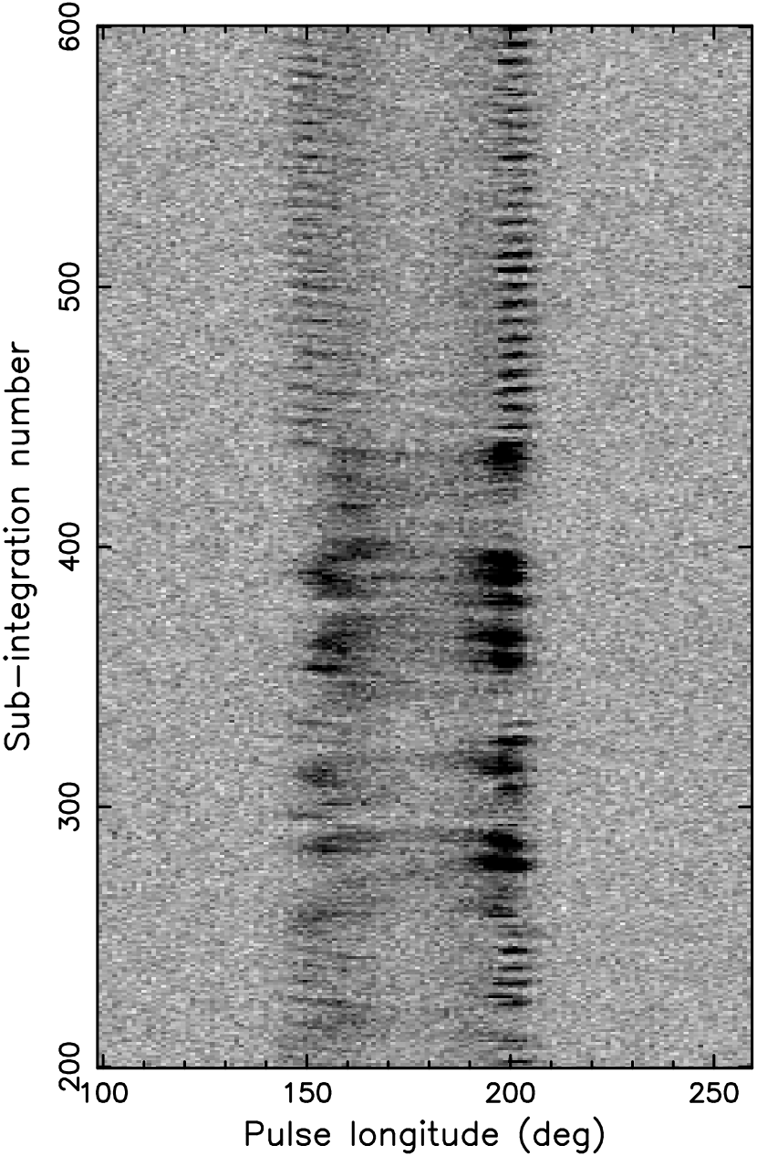
Figure 1: Pulse stack of PSR B1839–04. This is data set 2005a, rebinned into 300 pulse longitude bins. Every two pulses are summed together, so each subintegration contains the signal of two rotational periods. The data are clipped, meaning that all intensities above a certain threshold are set to that threshold value, thereby restricting the dynamic range. This makes the weaker features better visible.

PSRSALSA can visualise the data in various ways. In Fig. 1 a pulse stack is shown in grey-scale. The data shown in this figure are modified in several ways to emphasise the weaker emission features. To increase the signal-to-noise ($S/N$) ratio of each sample, the data were rebinned from 2246 to 300 pulse longitude bins. Secondly, since in the case of this pulsar the pulse shapes do not change too rapidly from pulse to pulse, each pair of pulses was summed, so that the first row in the figure is the sum of the first two pulses. These two steps greatly increase the $S/N$ per plotted intensity sample, hence improve the visibility of the pulse shape evolution. Finally, to make the organised patterns in the pulse stack even clearer, the data were clipped. This means that intensity values above a certain threshold were set to the threshold value. As a consequence, black regions in Fig. 1 which appear to have a uniform intensity, might in reality show some intensity variation. However, since the colour scale varies more rapidly over a narrower intensity range, intensity variations in weaker emission become much clearer.

Figure 1 shows several properties of the emission that are analysed in more detail later in this section. First of all, the emission is separated into a leading and trailing pulse longitude component that are referred to as components I ($\sim 140\degr-170\degr$) and II ($\sim 180\degr-210\degr$). These main profile components will be shown to be composed of two largely overlapping components themselves, resulting in components Ia, Ib, IIa, and IIb. Throughout this manuscript, including Fig. 1, the pulse longitude axis is defined such that component II peaks at $200\degr$, hence placing the saddle region between the two peaks approximately at $180\degr$.

The pulse stack shows that the emission of PSR B1839–04 is highly variable. Firstly, a clear periodic on- and off-switching is visible, which is clearest at the top of the figure from subintegration 450 and above. The bright emission phases are separated by approximately six subintegrations, hence 12 stellar rotations. This phenomenon is known as drifting subpulses, and the repetition period is referred to as $P_{3}$. Especially for component I, centred at pulse longitude $\sim 150\degr$, the bright emission phases appear as bands that are slightly diagonal in the figure, indicating that the bright emission “drifts” toward earlier times in subsequent stellar rotations. The emission bands seen in the trailing half of the profile are essentially horizontal with little evidence of drift, although for some bands a small tilt in the opposite direction compared to those in component I can be observed. These effects are quantified in Sects. 4.4 and 4.5.

Secondly, Fig. 1 shows that the subpulse behavior is distinctly different between subintegrations $\sim 250$ and $\sim 450$, indicating that two distinct emission modes operate in this pulsar. The mode referred to as the quiet mode (or Q mode) shows the regular and highly periodic subpulse modulation. However, during the more intense bright mode (B mode) the periodic subpulse modulation appears to be far less pronounced, or even absent. During the B mode the emission is not only brighter, components I and II are also closer to each other in pulse longitude with more emission in the saddle region. The modes are described in more detail in the next section.

4.2 Mode separation and concatenating data sets

To quantify the difference in the emission properties of the B and Q mode, the start and end pulse number of each mode was identified. Because of the variability caused by subpulse modulation, this process cannot easily be automated reliably. Instead, the classification was made by eye by interactively plotting the pulse stack using PSRSALSA, allowing smaller subsets of the data to be investigated efficiently. Identifying the mode transitions for this pulsar is a somewhat subjective process because of the intrinsic variability observed during a mode. Therefore it is often not clear with a single-pulse precision when a mode starts or ends. For instance, in Fig. 1 it might be argued that the B mode is interrupted for a short Q mode around subintegration 330, but it is hard to be certain. In addition, the transitions sometimes appear to be somewhat gradual, which could be because of the limited $S/N$ of the single pulses. To ensure that as much of the data as possible is labelled with the correct mode, some of the data were not assigned to either mode.

For all individual observations the fraction of rotations without an assigned mode was less than 10% (the average was 3%), except for the 2005c observation, for which 35% was in an undetermined mode. This was because the source was setting towards the end of the observation, resulting in an increase of the system temperature. Ignoring this observation, of the remaining 9195 rotations, 25% and 72% were assigned to the B and Q mode, respectively, with the remaining 3% being unclear. The median duration of a B and Q mode was 85 and 270 pulse periods, respectively.

To improve the $S/N$ of the following analysis, it is desirable to combine the data sets. PSRSALSA allows different observations to be concatenated, which was only done for the three 2005 data sets, since they have the same time resolution. The data sets were aligned in pulse longitude in a two-step process. First, an analytic description of the 2005a profile was obtained by decomposing the profile in von-Mises functions using PSRCHIVE. This allows PSRSALSA to align the data sets by cross-correlating this analytic description of the profile with the remaining two data sets. Since the profile is different during B and Q modes, the pulse profiles obtained by summing all pulses will vary from observation to observation. Therefore, the analytic template was based on the 2005a Q-mode pulses alone. The offsets in pulse longitude between the different data sets were determined by only cross-correlating the template with the Q-mode emission of all observations. The offsets obtained were applied to the full observations before concatenation.

During the process of concatenation, it is possible to specify that only multiples of a given block size defined in number of pulses are used from each data set. Similarly, when the mode separation was applied, it was possible to only use continuous stretches of data of the same specified length. This results in a combined data set that consists of blocks of continuous stretches of data of a given length, which is important when analysing fluctuation properties of the data with Fourier-based techniques (see Sect. 4.4).

Figure 2: Pulse profile of the different modes of PSR B1839–04. These are the combined 2005 data sets (the Q- and B-mode profiles consist of 7605 and 3188 individual pulses, respectively), rebinned with a factor two. The thick solid line and the long-dashed profile show the Q- and B-mode profiles, respectively. The peak flux of the B-mode profile is normalised and the Q-mode profile is scaled accordingly after taking into account the difference in number of pulses. The dotted profile is a scaled-down B-mode profile to aid a comparison between the shapes of the profiles in the two modes. The location of the four profile components are labelled.

Figure 2 shows the pulse profiles of the two modes. As expected, the B mode is brighter than the Q mode (compare the highest amplitude profile with the thick solid line). In addition, the saddle region of the profile is more pronounced in the B mode (compare the thick solid line with the dotted line, which is a scaled-down B-mode profile). As noted from an inspection of the pulse stack (Fig. 1), the two components are slightly closer together in the B mode. Figure 2 demonstrates that this is predominantly because the leading component shifts to later phases, although the trailing component also shifts slightly inwards. Especially the Q-mode profile shows that the main profile components show structure. In Fig. 2 four profile components are defined and labelled.

4.3 Pulse energy distribution

The difference in the brightness of the pulses in the two modes can be further quantified by analysing the so-called pulse energy distribution. The methods used here largely follow those described in Weltevrede et al. (2006b). The pulse energies were calculated for each individual pulse by summing the intensity values of the pulse longitude bins corresponding to the on-pulse region. The pulse energy distribution is shown in the inset of Fig. 3 together with an energy distribution obtained by summing off-pulse bins using an equally wide pulse longitude interval. Since the observations were not flux calibrated, the obtained pulse energies were normalised by the average pulse energy $\left<E\right>$.

Figure 3: Inset: The normalised pulse energy distribution of the combined 2005 data sets (solid histogram), and that of the off-pulse region (dotted histogram). The latter is scaled down by a factor three to make their amplitudes comparable. Main panel: The similarly normalised energy distribution of the Q (thin dashed histogram) and B mode (thick solid distribution) are shown separately. The fitted distribution functions are shown as the thin solid (B mode) and dashed curve (Q mode).

The pulse energy distribution including both modes shown in the inset of Fig. 3 shows no clear evidence for bi-modality. Bi-modality could have been expected since the distribution contains a mixture of bright and quiet mode pulses which, per definition, should have a different average brightness. The absence of bi-modality is a consequence of the significant pulse-to-pulse brightness variability observed during a mode, although random noise fluctuations can be expected to broaden the intrinsic energy distributions as well. The latter is quantified by the off-pulse distribution shown as the dotted histogram in the inset. The absence of clear bi-modality makes it hard to separate the modes in a more objective way than the method described in Sect. 4.2.

The energy distributions of the two modes are shown separately in the main panel of Fig. 3. The B-mode pulses are indeed brighter on average than the Q-mode pulses. As expected, the distributions significantly overlap. The cross-over point between the two distributions is located close to the average pulse energy $\left<E\right>$, which is where, in the overall energy distribution shown in the inset of Fig. 3, a small kink can be identified.

The distributions of both modes can be fairly well characterised by an intrinsic lognormal distribution convolved with the noise distribution. The lognormal distribution is defined to be

$$P(E/\left<E\right>)=\frac{\left<E\right>}{\sqrt{2\pi}\sigma E}\exp\left[-\left(\ln\frac{E}{\left<E\right>}-\mu\right)^{2}/\left(2\sigma^{2}\right)\right].$$ (1)

The parameters $\mu$ and $\sigma$ were refined in PSRSALSA using the Nelder-Mead algorithm (Nelder & Mead, 1965), which is an iterative process. For each iteration a large number of values of $E/\left<E\right>$ were drawn at random from the lognormal distribution. A randomly picked value from the off-pulse distribution was added to each value, resulting in a lognormal distribution convolved with the noise distribution. The goodness of fit used during the optimisation is based on a $\chi^{2}$ test using the cumulative distribution functions of the model and observed distribution and does therefore not depend on an arbitrarily chosen binning of the distributions. More detailed information about the method is available in the help of the relevant tools in PSRSALSA.

Table 2: Parameters quantifying the observed energy distribution of the Q and B modes after correcting for the effect of the noise distribution.

Mode	$\mu$	$\sigma$	KS prob.	Rejection significance
B	0.23	0.49	$1.4\times 10^{-1}$	1.5
Q	$-0.15$	0.44	$2.7\times 10^{-3}$	3.0

Table 2 lists the results of the fitting process. The overall goodness of fit after optimisation was quantified using the Kolmogorov-Smirnov (KS) test implemented in PSRSALSA (see e.g. Press et al. 1992 for a description of a similar implementation of the algorithm). It is a non-parametric test of the model and observed distribution, which does not require binning either. The null hypothesis is that the samples from both distributions are drawn from the same parent distribution. The probability that random sampling is responsible for the difference between the model and observed distributions can be estimated (hence a small probability means that the distributions are drawn from a different distribution). This probability can be expressed as a significance, in terms of a standard deviation of a normal distribution, of the rejection of the null hypothesis. In other words, a high significance means that the two distributions are likely to be different. The probability and significance are quoted in Table 2. Although the B mode is described with sufficient accuracy by a lognormal distribution, the fit of the Q-mode distribution is less accurate.

These results are consistent with the results of Burke-Spolaor et al. (2012), who also used a lognormal distribution to describe the observed energy distribution. A detailed comparison is not possible because Burke-Spolaor et al. (2012) neither separated the emission into different modes, nor did they convolve the model distribution with the noise distribution to obtain the intrinsic distribution. Nevertheless, their parameters are in between those derived for the B and Q modes in this work.

4.4 Fluctuation analysis

A sensitive method to determine time-averaged properties of the periodic subpulse modulation is the analysis of fluctuation spectra. The techniques described here are largely based on the work of Edwards & Stappers (2002), and for more details about the analysis, we also refer to Weltevrede et al. (2006a, 2007a, 2012). Two types of fluctuation spectra are exploited here, the first being the longitude-resolved fluctuation spectrum (LRFS; Backer 1970). The LRFS is computed by separating the pulse stack into blocks with a fixed length. As explained in more detail below, in this case, block lengths of either 512 or 128 pulses were used. For each block and each column of constant pulse longitude, a discrete Fourier transform (DFT) was computed, revealing the presence of periodicities for each pulse longitude bin. The final LRFS is obtained by averaging the square of the spectra obtained for the consecutive blocks of data.

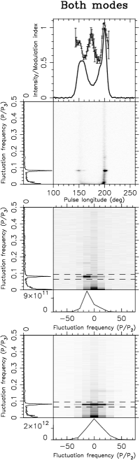
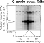
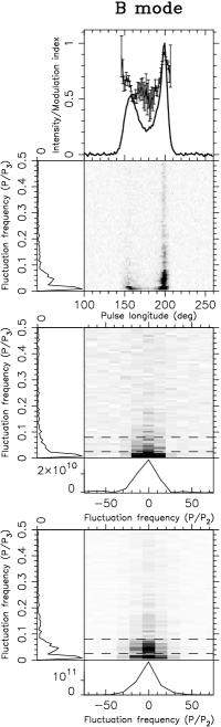
Figure 4: Fluctuation analysis of the emission including both modes of PSR B1839–04, and those of the Q and B mode separately. These are the combined 2005 data sets, rebinned with a factor 9 in pulse longitude. Top row: The pulse profile and the modulation index (points with error bars). Second row: The LRFS and a side panel showing the horizontally integrated power. Third row: The 2DFS of component I and side panels showing the horizontally (left) and vertically, between the dashed lines, integrated power (bottom). Bottom row: The 2DFS of component II. Third column: The 2DFS of Q-mode emission of component II with an adjusted vertical range and grey-scale emphasizing the second harmonic.

The fluctuation analysis was made for the Q and B modes separately, and for both modes combined. To achieve the highest $S/N$, the combined 2005 data sets were used. However, it is important to ensure that the combined data set consists of an integer number of blocks with an equal number of single pulses $n_{\mathrm{dft}}$ each, where $n_{\mathrm{dft}}$ is the length of the DFTs used to compute the fluctuation spectra. This ensures that the single pulses used in each DFT are continuous. For the left column of Fig. 4, which shows the results of the fluctuation analysis before mode separation, $n_{\mathrm{dft}}$ was set to 512 pulses to achieve a relatively high frequency resolution. Since this implies that only a multiple of 512 pulses could be used, some of the recorded pulses of each 2005 data set were not included in the analysis (resulting in 11776 analysed pulses). The fluctuation analysis of the individual modes was hampered by the fact that the mode changes occur too often to find long enough stretches of data without a mode switch. Therefore $n_{\mathrm{dft}}$ was reduced to 128 consecutive pulses for the mode-separated data. Next, some general results for the non-mode-separated data are summarised and the methods used are explained. This is followed by the results of the mode-separated data.

4.4.1 Non-mode-separated data

In Fig. 4 the top panels show the pulse profile (solid curve). The panel below shows the LRFS in grey-scale, which is aligned in pulse longitude with the panel above. The side panel of the LRFS of the whole data set (first column) shows a clear spectral feature at $P/P_{3}\simeq 0.08$ cycles per period (cpp). This spectral feature corresponds to the pattern repetition period of the drifting subpulses $P_{3}\simeq 12P$ that was identified by eye in the pulse stack (Fig. 1). The narrowness of the spectral feature (high quality factor) indicates that the periodicity is well defined. The LRFS itself shows that most of this periodic modulation power is associated with the outer halves of the two main components where most of the spectral power is detected (darker colour), that is, components Ia and IIb corresponding to pulse longitudes $145\degr-155\degr$ and $195\degr-205\degr$. As mentioned before and illustrated further in Sect. 4.5, this suggests that the two main profile components are double themselves, resulting in at least four distinct profile components. Although much weaker, the second harmonic at $\sim 0.16$ cpp is detected as well.

In addition to this well-defined spectral feature, a weak white noise component is most clearly seen as the vertical darker band in the LRFS centred at pulse longitude $\sim 200\degr$. This indicates non-periodic random fluctuations. A red-noise-like component is strongest below $P/P_{3}=0.02$ cpp, corresponding to fluctuations on a timescale of 50 pulse periods and above.

The power in the LRFS can be used to quantify the longitude-resolved modulation index, which is shown as the points with error bars in the top panels of Fig. 4 together with the pulse profile. This is a measure for the amount of intensity variability (standard deviation), normalised by the average intensity at a given pulse longitude. An advantage of computing the modulation index through the spectral domain is that for instance periodic radio frequency interference (RFI), which affects a specific spectral channel, can be masked, thereby removing its effect on the modulation index. In addition, the effect of white noise as determined from the off-pulse region, resulting from a finite system temperature, for instance, can be subtracted from the measured modulation index.

PSRSALSA can determine the error bar on the modulation index using a method analogous to that used by Edwards & Stappers (2002), or through bootstrapping, which generally results in more reliable (although conservative) errors (see Weltevrede et al. 2012 for details). A pure sinusoidal drifting subpulse signal would result in a modulation index of $1/\sqrt{2}\simeq 0.71$. Since both lower and higher values are observed at different pulse longitude ranges (see Fig. 4), the presence of both non-fluctuating power and additional non-periodic intensity fluctuations can be inferred. Burke-Spolaor et al. (2012) found the minimum in the longitude-resolved modulation index of PSR B1839–04 to be $1.12$, significantly higher than what is shown in Fig. 4. This is most likely because the authors included system-temperature-induced white noise in the result (private communication).

The LRFS is a powerful tool to identify any periodically repeating patterns as a function of pulse longitude, but it cannot be used to identify if the emission drifts in pulse longitude from pulse to pulse (i.e. drifting subpulses). If drifting subpulses are present, the pattern of the emission in the pulse stack resembles a two-dimensional sinusoid. This makes the two-dimensional fluctuation spectrum (2DFS; Edwards & Stappers 2002) especially effective in detecting this type of pattern since most modulation power is concentrated in a small region in this spectrum.

The 2DFS was computed for components I and II separately, resulting in the grey-scale panels in the one but last and last rows in Fig. 4, respectively. Like for the LRFS, the vertical frequency axis of the 2DFS corresponds to $P/P_{3}$, and the spectra for both components show the same $P_{3}\simeq 12P$ pattern repetition periodicity as identified in the LRFS. The horizontal axis of the 2DFS denotes the pattern repetition frequency along the pulse longitude axis, expressed as $P/P_{2}$, where $P_{2}$ corresponds to the separation between the subpulses of successive drift bands in pulse longitude, that is, their horizontal separation in Fig. 1. The first 2DFS in the left column of Fig. 4 shows that the power corresponding to the drifting subpulses (found at $P/P_{3}\simeq 0.08$ cpp between the dashed lines) is asymmetric, such that most of the power is concentrated in the left-hand half of the spectrum. This indicates that the subpulses move towards earlier pulse longitudes from pulse to pulse. The power peaks at $P/P_{2}\simeq-15$ cpp, suggesting that $P_{2}\simeq 360\degr/15\simeq 25\degr$. This implies that the drift bands in component I have a drift rate (slope in the pulse stack) $P_{2}/P_{3}\simeq 2\degr$ per $P$ and thus that the subpulses drift. The 2DFS of the trailing component shows again clear $P_{3}$ modulation, but the spectral feature is much more centred on the vertical axis. This suggests that if the subpulses do drift in pulse longitude, $P_{2}$ will be much larger for the trailing component, corresponding to more horizontal drift bands in the pulse stack. This is consistent with Fig. 1, which showed little evidence for drift in component II.

4.4.2 Mode-separated data

The second and last column of Fig. 4 show the results of the same type of analysis, but now for the mode-separated data. As discussed before, it is important to use blocks of continuous stretches of data with a length determined by $n_{\mathrm{dft}}$. Since the modes only last for a certain amount of time, the amount of usable data decreases the larger $n_{\mathrm{dft}}$ is. For this reason a reduced $n_{\mathrm{dft}}$ of 128 pulses was used for the mode separated data. The Q- and B-mode analysis is based on all available continuous stretches of 128 pulses in a given mode found in each of the 2005 data sets, resulting in 6016 and 896 available pulses for the Q and B mode, respectively. The spectra of the Q mode clearly show the $P_{3}\simeq 12P$ periodic subpulse modulation, while this feature is absent from the B-mode data. On the other hand, the B mode shows a low-frequency red-noise component that is absent during the Q mode. This clearly indicates that the features in the spectra seen in the first column of Fig. 4 are the superposition of features seen in the two modes.

Weltevrede et al. (2006a) measured $P_{2}$ and $P_{3}$ from the 2DFS by calculating the centroid of a region in the 2DFS containing the drifting subpulse feature, which therefore does not rely on any assumption about the shape of the feature. The associated uncertainties are typically the combination of three effects. First of all, there is a statistical error caused by white noise in the data (hence in the 2DFS), resulting in an uncertainty in the centroid calculation. Typically, this error can be neglected because there is a larger systematic error associated with the somewhat subjective choice of which rectangular region in the 2DFS to include in the centroid calculation. This error can be estimated in PSRSALSA by using an interactive tool that allows the user to select a rectangular region in the 2DFS after which the centroid and statistical error is determined. By repeating this process a number of times by making different selections, this systematic error can be quantified. The third contribution to the uncertainty is that pulsar emission is in practice inherently erratic in the sense that if a certain feature is statistically significant for a certain data set, it still might not be an intrinsic (reproducible) feature of the pulsar emission. This is always an issue when analysing a limited data set that is too short to determine the true average properties of the pulsar emission. To assess the importance of this effect, the data set could be split in different ways to see if the same feature is persistent. In addition, the order of the pulses can be randomized to determine the strength of any apparent “significant” periodic features, which in this case clearly must be the result of having a finite data set. For PSR B1839–04, the features reported here are confirmed in all data sets, ensuring that they truly reflect intrinsic properties of the pulsar emission.

After taking the above systematics into consideration, Weltevrede et al. (2006a) reported (based on the 2003 observation) that components I and II show periodic modulation with $P_{3}=12.4\pm 0.3\;P$ and $P_{2}=-35^{+5}_{-15}$ and $120^{+20}_{-20}$ degrees, respectively. Note in particular the sign difference in the two $P_{2}$ values, implying that the subpulses drift towards earlier phases in component I, but in the opposite direction for component II. This is referred to as bi-drifting and the existence of this phenomenon has important theoretical consequences. The claim for bi-drifting was based on a lower $S/N$ equivalent of the plot in the first column (not mode-separated data) of Fig. 4. The $P_{2}$ value of the leading component is convincingly negative (see bottom side-panel of the first 2DFS, which shows that the vertically integrated power between the two dashed lines clearly peaks at a negative $P_{2}\simeq-15$ cpp. Bi-drifting should result in a feature at the same $P_{3}$ in the second 2DFS (bottom row of Fig. 4), which is offset in the opposite direction. This is not immediately obvious from the spectrum (even with the greatly increased $S/N$), since the power peaks at 0 cpp, suggesting no drift at all. Nevertheless, utilising the centroid method outlined above, it is found that $P_{3}=12.4\pm 0.2\;P$ and $P_{2}=-35^{+7}_{-5}$ degrees for component I and $P_{3}=12.4\pm 0.1\;P$ and $P_{2}=260^{+60}_{-10}$ degrees for component II. These measurements are consistent with those by Weltevrede et al. (2006a) and confirm the slight offset of the centroid of the feature in the 2DFS of the second component, resulting in the claim of bi-drifting. However, given the importance of the claim, and the level of uncertainty in the errors, more convincing evidence is highly desirable.

By exploiting the high $S/N$ of the combined 2005 data, further evidence for bi-drifting comes from analysing the second harmonic in the 2DFS of component II. This harmonic is shown more clearly in the third column of Fig. 4, which only shows the bottom half of the 2DFS with the brightest features clipped to emphasize the weaker features. This harmonic should be located twice as far from the origin than the fundamental, that is, $P/P_{3}$ and $P/P_{2}$ can be expected to be twice as large. Especially the increased offset from the vertical axis helps greatly since the resolution in $P/P_{2}$ is relatively poor. As clearly demonstrated by the bottom side-panel, the integrated power between the dashed lines is asymmetric with an excess at positive $P_{2}$, convincingly confirming bi-drifting. The centroid position of the second harmonic was determined to be $P_{3}=6.1\pm 0.2\;P$ and $P_{2}=50^{+60}_{-2}$ degrees, consistent with the measurements based on the fundamental. The separate 2005 data sets show a similar second harmonic (not shown), and even the 2003 data analysed by Weltevrede et al. (2006a) weakly show the same feature. Although the detection of a second harmonic was mentioned by Weltevrede et al. (2006a), its offset from the vertical axis was neither measured nor used.

4.5 Subpulse phase analysis

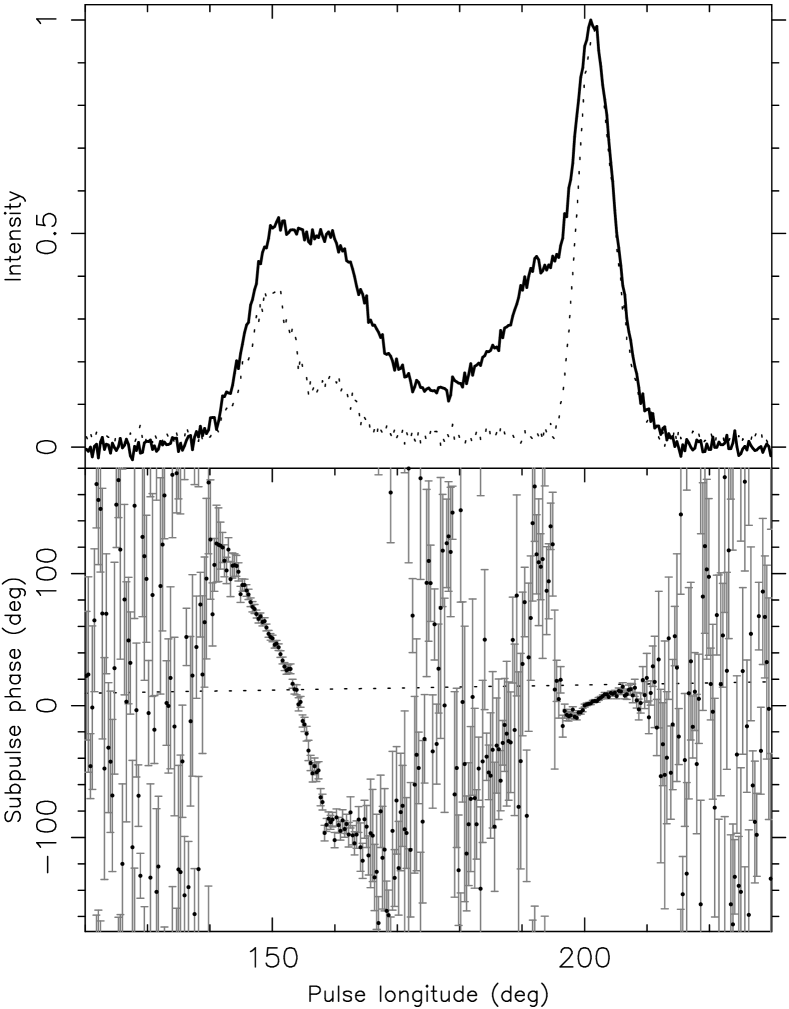
Figure 5: These are the combined 2005 Q-mode data rebinned with a factor of 2. Upper panel: The strength of the $12P$ modulation pattern as a function of pulse longitude (dotted curve) and the pulse profile (black curve). Lower panel: The corresponding subpulse phase. An arbitrary phase offset has been applied to make the subpulse phase zero at the peak of the profile. The dotted line indicates the gradient of the phase relation expected for a modulation pattern that is longitude stationary in the co-rotating pulsar frame.

Although the 2DFS is very effective in detecting drifting subpulses in noisy data, it does not allow easy characterisation of all the relevant average properties. In particular, there is only limited information about their pulse longitude dependence, including for instance the phase relation of the modulation cycle as observed in different components. Following Edwards & Stappers (2002) and as explained in Weltevrede et al. (2012), PSRSALSA allows this phase relation as a function of pulse longitude to be extracted using spectral analysis. This information, as shown in Fig. 5, is obtained by first of all computing the LRFS for the Q-mode data of the combined data set. Relatively short DFTs were used: $n_{\mathrm{dft}}=64$ pulses. This ensured that the majority of the power associated with the drifting subpulses was concentrated in a single spectral bin. In addition, this allowed more blocks of consecutive pulses in the Q mode to be analysed: 6720 pulses in total.

The LRFS as discussed in Sect. 4.4 was constructed by taking the square of the complex values obtained from the DFTs, while here the complex phase was considered as well. The complex phase is related to the subpulse phase, while the magnitude of the complex values is related to the strength of the drifting subpulse signal. A difference in subpulse phase obtained for two pulse longitude bins quantifies the difference in phase of the modulation pattern at those two longitudes. In other words, if there is no phase difference, the subpulse modulation pattern is in phase in the sense that the maximum brightness occurs at the same pulse numbers (which is often referred to as longitude stationary modulation).

Here the spectral bin centered at 0.078125 cpp was analysed, which contains most of the subpulse modulation. The complex phase will be different for the subsequent blocks of data because $P_{3}$ will be variable over time. As a consequence, a process is required to coherently add the complex numbers obtained for the subsequent blocks of data. The required phase offsets are independent of pulse longitude, but vary from block to block. The iterative process used to obtain these phases maximises the correlation between the phase profiles of the different blocks in the on-pulse region. The coherent addition results in the complex subpulse modulation envelope, with a complex phase corresponding to the subpulse phase. Error bars were determined by applying a similar method to that used to determine the uncertainties on the modulation index. In addition to the complex phase of the resulting complex modulation envelope, its amplitude is also obtained (see also Edwards & Stappers 2002; Edwards et al. 2003). The resulting subpulse amplitude envelope as calculated with PSRSALSA is normalised such that it would be identical to the normalised pulse profile if the subpulse modulation were sinusoidal with a frequency $P/P_{3}$ equal to that of the spectral bin analysed. The actual measured amplitude depends on the presence of non-modulated power, the stability of the subpulse phase differences between pulse longitude bins, and the accuracy of the determined offsets used to do the coherent addition.

Figure 5 shows the results of this analysis. For component I the subpulse phase decreases with pulse longitude. In the sign convention used here (and in Weltevrede et al. 2007b, 2012), this corresponds to negative drift, that is, drift towards earlier pulse longitudes. The slope of the subpulse phase track is opposite for the trailing component, confirming the bi-drifting phenomenon.

The top panel of Fig. 5 shows that the subpulse amplitude profile is high in both the leading part of the leading half of the profile (component Ia) and especially the trailing part of the trailing half of the profile (component IIb). The subpulse amplitude profile shows component Ib as a more distinct component compared to the intensity profile. This again suggests that the pulse profile should be considered to be composed of four components: two pairs of components that are blended to form the roughly double-peaked pulse profile as indicated in Fig. 2. This could be interpreted as the line of sight making a relatively central cut through a nested double-conal structure, with the modulation being strongest in the outer cone.

Interestingly, the subpulse phase at the trailing end of component Ib becomes longitude stationary, more like what is observed for component IIb. In the bridge region between the two emission peaks the error bars on the subpulse phase are large, partly because the errors are somewhat conservative, but mainly because the emission barely shows the $12P$ modulation. Nevertheless, there appears to be a clustering of subpulse phase points that smoothly connects the subpulse phase tracks observed for the strongly modulated outer components. Possible relatively sharp deviations are observed at pulse longitudes $\sim 177\degr$ and $\sim 192\degr$.

When interpreting the subpulse phase as a function of rotational phase, it should kept in mind that if the pulsar generates a modulation pattern that is longitude stationary in the pulsar (co-rotational) frame, that is, a pure intensity modulation without any drift, the observer will still observe an apparent drift (e.g. Weltevrede et al. 2007b). This is because for a given pulse number, a later pulse longitude is observed later in time, which means that a later part of the modulation cycle will be observed. An intrinsically pure intensity modulation will therefore result in a slow apparent positive drift (i.e. emission appearing to drift toward later phases). This drift rate is indicated by the dotted line in the lower panel of Fig. 5, which has a gradient of $P/P_{3}$ degrees of subpulse phase per degree of pulse longitude.

4.6 Phase-locking

As we discuss in Sect. 6, bi-drifting can be more easily explained if the modulation cycle observed in the two profile components operate, at some level, independent of each other. It is therefore important to determine if the two modulation cycles are phase locked, meaning that if the modulation cycle slows down in the leading component, it is equally slow in the trailing component, such that the modulation patterns of both components stay in phase. Phase-locking can be expected for PSR B1839–04 given that the subpulse amplitude in Fig. 5 is high for both components. This would only occur if the subpulse phase relationship with pulse longitude as shown in the lower panel is fixed over time. Phase-locking is confirmed by computing and comparing the subpulse phase profiles of the Q-mode data of the individual observations listed in Table 1. The shape of the subpulse phase profile, including the phase delay between the components, is the same for the separate observations (not shown), confirming that strict phase-locking is maintained over a period of years. This strongly suggests that the modulation patterns in both components have a single physical origin.

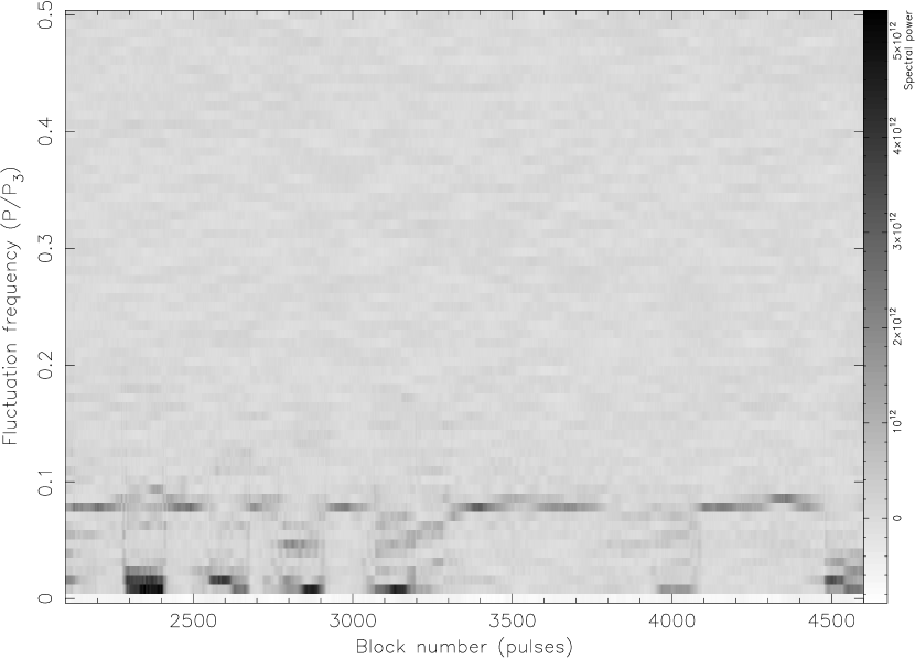
Figure 6: Part of the S2DFS of observation 2005a of PSR B1839–04, showing spectral power as a function of pattern repetition frequency in component II and time (defined as the start pulse number of the 128 pulses long sequence of pulses used to determine the spectral power). Transitions from the Q mode, during which there is a strong $P/P_{3}=0.08$ spectral feature, to the B mode, during which low-frequency modulation dominates, are evident.

As noted before, the spectral features in the LRFS have a high quality factor, suggesting a relatively stable periodicity. Nevertheless, we observe significant broadening. The variability of $P_{3}$ can be demonstrated more directly by exploiting the Sliding 2DFS (S2DFS; Serylak et al. 2009), which has temporal resolution. The S2DFS is obtained by computing the 2DFS for separate blocks of data (here component II, for which both the modulation and intensity are strongest), where the block-size is $n_{\mathrm{dft}}$ pulses of data. The first block analysed contains the first $n_{\mathrm{dft}}$ pulses, and successive blocks start one pulse later. Therefore, the results for each block are not independent of each other. The spectra obtained for each block were integrated over $P_{2}$, resulting in Fig. 6. See Serylak et al. (2009) for a full description of the method.

Figure 6 clearly shows mode changes between the Q mode (strong spectral power at $P/P_{3}=0.08$ cpp) and B mode (strong spectral power at lower frequencies). However, since the resolution is limited by $n_{\mathrm{dft}}$ pulses, this method cannot be used to separate the modes more accurately than the method described in Sect. 4.2. Despite the somewhat limited fluctuation frequency resolution defined by $n_{\mathrm{dft}}$, the fluctuation frequency is observed to be variable (see for example the increase in fluctuation frequency at block number 4300).

The magnitude of the variability was quantified for the Q mode by fitting the curves shown in Fig. 4 in the left side-panels of the 2DFS of both profile components. The spectral feature was fit with a Gaussian function, while the background was described by a second-order polynomial. The $P/P_{3}=0$ bin and all bins above and including the second harmonic were excluded. Although not perfect, a Gaussian fit was deemed accurate enough to define the width. We found that the width of the spectral feature, hence the magnitude of the observed variability in $P_{3}$, is within the errors identical in both components (the ratio is $1.07\pm 0.06$). This is expected since phase-locking implies that the magnitude of the variations in $P_{3}$ is the same in the two components.

4.7 $P_{3}$-fold

So far, the subpulse modulation of PSR B1839–04 has been detected and quantified using Fourier based techniques. A completely independent method to visualise the time-averaged properties of subpulse modulation is by folding the data at the period $P_{3}$. $P_{3}$-folding essentially averages the pulse stack over the modulation cycle, resulting in the average drift band shape without assuming a sinusoidal modulation pattern. A complication is that $P_{3}$ is variable throughout the observation, hence the fluctuations in $P_{3}$ have to be detected and compensated for. This allows longer stretches of data to be folded, without the modulation cycle being smeared out because of misaligned modulation cycles during the averaging process. Since the spectral feature in the LRFS is indeed smeared out over a finite range of $P_{3}$ (see Figs. 4 and 6), this correction can be expected to be essential to obtain a satisfactory result for PSR B1839–04. $P_{3}$-folding has been done before, but without resolving the $P_{3}$ variations (e.g. Deshpande & Rankin 2001; Edwards et al. 2003). The same algorithm as described below was used by Hassall et al. (2013).

The process of $P_{3}$-folding starts with specifying the $P_{3}$ value used for the folding, here taken to be $12.4P$ as measured in Sect. 4.4.2. Here, the 2005 data in the Q mode were analysed. In PSRSALSA, the basic approach to fold the data is to separate out blocks of continuous pulses (in this case taken to have a length of 37 pulses, or about three modulation cycles). Then each block is folded with the specified $P_{3}$ value (fixed-period folding). The variability in $P_{3}$ is taken into account by finding appropriate phase offsets as explained below. Analogous to what is done for the fluctuation analysis, only stretches of continuous data with a duration of a multiple of 37 pulses were used to ensure that the pulses in each block of data being analysed is continuous (resulting in 7141 usable pulses). Increasing the block-size would increase the accuracy to correct for $P_{3}$ variability because of the increased overall $S/N$ per block. However, an increased block size will result in a pattern that is more smeared out because the fixed-period folding is not accurate enough within a block of data, hence a compromise needs to be made.

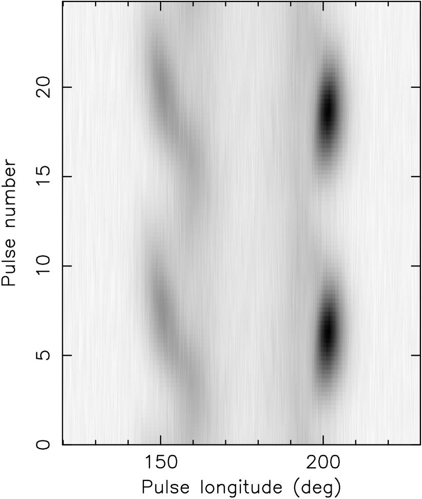
Figure 7: $P_{3}$-fold of the added 2005 data of PSR B1839–04 in the Q mode. The average $P_{3}=12.4P$ modulation cycle is shown twice for continuity.

The variations in $P_{3}$ are resolved by an iterative process during which the modulation patterns obtained for the individual blocks of data are compared, resulting in their relative offsets. This means that if $P_{3}$ is slightly larger than the typical value specified, the drift band will appear slightly later in the second block than in the first. Hence when folding the data, this additional offset has to be subtracted first. These offsets are determined by cross-correlating the modulation pattern of the blocks of data and a template. Only the on-pulse region, containing signal, was used to correlate to determine the offsets, but the full pulse longitude range is folded. Since the cross-correlation relies on knowledge about the shape of the modulation pattern, an iterative process is required. During the first iteration this knowledge is not available, hence the modulation pattern of the first block of data is used to determine the offset of the second block of data. After coherent addition, this result is used to determine the offset of the third block, etc. After folding the full data set using these offsets, the result is the “average drift band”. However, the determined offsets can be refined by using this high $S/N$ average drift band as a template to compute new cross-correlations, allowing more precise offsets to be determined for each block. In total, four iterations were used to calculate Fig. 7. The result is shown twice on top of each other for continuity.

The intrinsic resolution of the $P_{3}$-fold is one pulse period, but “oversampling” could give a cosmetically improved display of the result. This means specifying more than $P_{3}/P$ bins covering the modulation cycle, resulting in bins that are not completely independent of each other. Here the $P_{3}$ cycle was divided into 50 equally spaced bins. A given pulse was added to each of the 50 bins during the averaging process after applying a weight from a Gaussian distribution with a standard deviation of 4 bins and an offset corresponding to the difference between the expected modulation phase of the given pulse and that of the bin. This Gaussian smoothing effectively makes the obtained resolution of the modulation cycle equal to one pulse period.

Figure 7 shows the resulting $P_{3}$-fold in which the power is concentrated in two pulse longitude ranges corresponding to components Ia and IIb. The leading component clearly shows negative drift, that is, subpulses moving towards the leading edge. The power in the trailing peak does not clearly show drifting, consistent with the fact that the drift-rate should be much lower. Nevertheless, the figure reveals that there is drift such that at the trailing side the pattern is brighter at later times (higher up along the vertical axis). This is confirmed by analysing the centroid of the power in each column as a function of pulse longitude. This confirms that indeed subpulses drift in opposite directions in components Ia and IIb using a completely different method independent of Fourier techniques.

5 Polarization

Radio polarization, in particular the observed position angle (PA) of the linear polarization, can be used to constrain the magnetic inclination angle $\alpha$ of the magnetic axis and the inclination angle $\zeta$ of our line of sight with respect to the rotation axis. Here we apply the methodology described in Rookyard et al. (2015) and implemented in PSRSALSA on the 1408 MHz polarimetric pulse profile of PSR B1839–04 published by Gould & Lyne (1998), which is made available through the European Pulsar Network Data Archive, to derive robust constraints after systematic consideration of the relevant uncertainties.

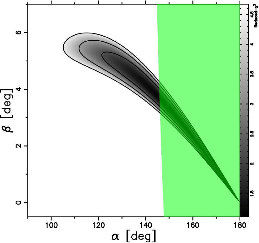
Figure 8: Top panel: Polarimetric pulse profile of PSR B1839–04 observed at 1408 MHz (Gould & Lyne, 1998) showing total intensity (solid line), linear polarization (dashed line) and circular polarization (dotted line). Below the profile the PA measurements are shown with the solid curve showing the best fit of the RVM. Lower panel: The goodness-of-fit of the RVM is shown in grey-scale, with the contours corresponding to 1, 2, and $3\sigma$ levels. For the green area of the graph the observed pulse width is consistent with considerations of the expected beam size for this pulsar (see main text).

The top panel of Fig. 8 shows the polarimetric profile as derived by PSRSALSA from the recorded Stokes parameters. By default the amount of linear polarization is computed using the method described in Wardle & Kronberg (1974). The PA points are only shown and used when the linear polarization exceeds three times the standard deviation as observed in the off-pulse region.

The pulse longitude dependence of the observed PA (i.e. PA-swing) can be related to $\alpha$ and $\zeta$ through the rotating vector model (RVM; Radhakrishnan & Cooke 1969; Komesaroff 1970). The observed PA-swing can be explained well with this model, as shown in the top panel of Fig. 8 and is quantified by the reduced $\chi^{2}$ of 1.2. The geometrical parameters of the RVM are not well constrained by the PA-swing, which is, as is often the case, limited by the duty cycle of the profile. The degeneracy in the model parameters is quantified in the lower panel of Fig. 8, which shows the goodness-of-fit of the RVM as function of $\alpha$ and $\beta$, where $\beta=\zeta-\alpha$ is the impact parameter of the line of sight with respect to the magnetic axis. The black contours correspond to $\chi^{2}$ levels that are two, three, and four times higher than the lowest reduced-$\chi^{2}$, equivalent to the 1, 2 and $3\sigma$ levels. It can be seen that $\beta$ is constrained to be positive, corresponding to a positive gradient of the PA-swing. The fact that $\alpha$ is constrained to be larger than $90\degr$ means for a positive $\beta$ that there is an “inner” line of sight, or in other words, that the line of sight passes in between the rotational and magnetic axis.

Table 3: Measured parameters used to obtain the green region as indicated in Fig. 8.

$\phi_{\mathrm{left}}$	$\phi_{\mathrm{right}}$	$\phi_{\mathrm{fid}}$	$\phi_{\mathrm{0}}$
[deg]	[deg]	[deg]	[deg]
$141.5\pm 2.9$	$208.5\pm 1.6$	$175\pm 25$	$174.9^{+0.5}_{-0.4}$

Rookyard et al. (2015) provided a more elaborate discussion about the used RVM fit methodology and also discussed how beam opening angle considerations in combination with constraints on aberration and retardation effects and the observed pulse width can be used to obtain a further constraint on $\alpha$ and $\beta$. The relevant input parameters and their uncertainties can be found in Table 3. Here the pulse longitude of the left and right edge of the pulse profile are defined at the 10% peak intensity level and the error bars are determined from the difference with those at the 20% level. The fiducial plane position, the pulse longitude corresponding to the line of sight being closest to the magnetic axis, was set to the mid-point between the left and right edge of the profile. Since the profile is not perfectly symmetric, this is a somewhat subjective choice. To account for a possible partially active open field line region, the uncertainty was taken to be relatively large such that the range of fiducial plane positions includes the position of the two main profile peaks. This would allow for a “missing” component either before or after the observed profile. Following the procedure outlined in Rookyard et al. (2015), only a subsection of parameter space as indicated by the green region in Fig. 8 is consistent with the predicted open field line region of a dipole field.

Figure 8 suggests that $\alpha$ is likely to be relatively small (i.e. close to $180\degr$). The magnetic inclination angle is likely to be smaller than $35\degr$. This is because the observed pulse width is relatively wide ($w_{10}=67\degr$), while there is no evidence for a large emission height from the offset between the fiducial plane position and the inflection point of the PA-swing (Blaskiewicz et al., 1991). In fact, the measured value of the inflection point slightly precedes the assumed fiducial plane position, although not significantly so. Since the opposite is expected, it suggests that if the fiducial plane position is close to the defined central point in the pulse profile, the emission height should be low. In that case the pulsar will be a relatively aligned rotator with $\alpha$ close to $180\degr$. A small inclination angle is consistent with the analysis of Wu et al. (2002), for instance, who found $\alpha=7.4\degr$ without a defined uncertainty.

6 Discussion

In this section the bi-drifting phenomenon is discussed by first of all comparing the two known bi-drifters. Explaining these results is challenging, and a range of ideas, some specifically proposed in the literature as a model for bi-drifting, are argued to be implausible. Finally, potential ways to avoid these theoretical problems are identified.

6.1 Comparison with PSR J0815+0939

As noted above, bi-drifting was reported for one more pulsar: J0815+0939 (McLaughlin et al., 2004; Champion et al., 2005). With a shorter period ($P=0.645$ seconds), but an almost four times higher spin-down rate, the characteristic age of PSR J0815+0939 ($\tau_{c}=74$ Myr) is similar to that of B1839–04 ($\tau_{c}=57$ Myr). This places both pulsars at the lower spin-down rate end of the distribution of known pulsars in the $P-\dot{P}$ diagram. Nevertheless, their spin-down properties are by no means exceptional, making it unlikely that spin-down parameters alone determine if pulsars show bi-drifting.

In addition to the bi-drifting, another interesting feature about PSR J0815+0939 is its distinct pulse profile shape at a frequency of 327 and 430 MHz, which has four very clearly separated components with deep minima between them (Champion et al., 2005). However, at 1400 MHz the profile is comparable to that of PSR B1839–04 at a similar frequency, with overlapping profile components resulting in a much more double-peaked structure. At 408 MHz the profile of PSR B1839–04 shows no evidence for a similar frequency evolution as J0815+0939 (Gould & Lyne, 1998), although it cannot be ruled out that at even lower frequencies something similar might occur. Nevertheless, our analysis does show the presence of four profile components in the profile of PSR B1839–04.

The profile of PSR J0815+0939 is more narrow when expressed in seconds. Champion et al. (2005), for example, reported ${w_{10}=183}$ ms at 430 MHz. However, it is more relevant that its duty cycle is very large, almost 28% and slightly more at 1400 MHz. This is even larger than the duty cycle measured here for PSR B1839–04 at 1380 MHz (19%). This suggest that PSR J0815+0939 is a relatively aligned rotator, similar to PSR B1839–04. A difference is that the profile of PSR J0815+0939 appears to narrow at lower frequencies, while that of PSR B1839–04 widens (e.g. Chen & Wang 2014).

Subpulse modulation is observed for all four components of PSR J0815+0939. The first component has an unclear drift sense (appears to change during observations). The second component has positive drift, while the remaining components have negative drift. This feature is reported to be stable from observation to observation (Champion et al., 2005). It must be noted that a more detailed analysis of the first component of PSR J0815+0939 might reveal if there is any systematic drift direction detectable. Therefore it is unclear if the first component of PSR J0815+0939 is comparable with the second component of PSR B1839–04 in the sense that at first glance the drift sense is unclear. The bi-drifting in both pulsars is consistent with a symmetry such that the drift sense is opposite in the two halves of the profile, but the same within a given half of the profile. This could well be a generic feature of the bi-drifting phenomenon.

6.2 Basic requirements for a model for bi-drifting

Any model for bi-drifting should be able to explain at least the following basic observed properties.

1. Why different profile components can have subpulses drifting in opposite directions.

2. Why this is so uncommon in the overall pulsar population.

3. Why $P_{3}$ is the same in the different components.

4. How very strict phase-locking of the modulation cycle in different components can be maintained.

Especially the last point is a critically difficult property to be explained by emission models. Phase-locking is explicitly demonstrated here for PSR B1839–04 over a timescale of years. In addition, it is unaffected by disruptions by mode changes.

6.3 Theoretical difficulties in interpreting bi-drifting

As mentioned in the introduction, a widely used model to explain drifting subpulses is the carousel model. This is a specific physical model based on circulation of pair-production sites (known as sparks), responsible for beamlets of radio emission. The circulation around the magnetic axis is caused by an $\bm{E}\times\bm{B}$ drift. Although much of the following discussion is described in terms of this model, the arguments in this subsection apply equally to any model that tries to explains drifting subpulses by a circulation of radio beamlets around the magnetic pole.

6.3.1 Oppositely circulating nested beamlet systems

Qiao et al. (2004b) argued, motivated by the results for PSR J0815+0939, that bi-drifting can be explained in the context of the inner annular gap (IAG) discussed by Qiao et al. (2004a). Within the framework of the Ruderman & Sutherland (1975) model, particle acceleration is expected in the charge-depleted region in the open field line zone close to the neutron star surface (polar gap). This polar gap is divided into two regions: a central region (the inner core gap; ICG) above which the charge density of the magnetosphere has an opposite sign compared to that above the annular region surrounding it (IAG). The IAG is likely to require the star to be a bare strange star in order for it to develop. It was argued by Qiao et al. (2004b) that a carousel of sparks could exist in both regions, each rotating in an opposite sense. This provides the physical basis for different components having opposite drift senses.

As pointed out by van Leeuwen & Timokhin (2012), the Ruderman & Sutherland (1975) model without the addition of an IAG does not necessarily imply that only one sense of carousel rotation is allowed. Therefore without invoking emission from the IAG, two nested beamlet systems rotating in opposite directions could be considered. The arguments made below about the Qiao et al. (2004b) model therefore equally apply to such a model, or any model based on circulation occurring in opposite directions.

In its most simple form, this model would predict that there is a pair of inner components with the same drift sense, and an outer pair both having the same drift sense (opposite from the inner pair). This is inconsistent with the patterns observed for both bi-drifting pulsars. Therefore a symmetry-breaking mechanism needs to be invoked to change the natural symmetry implied by the IAG model. Qiao et al. (2004b) proposed that emission produced at multiple emission heights in combination with delays arising from retardation and aberration could be responsible. For PSR J0815+0939 it was proposed that for both the IAG and ICG radio emission is generated at two separate heights, giving effectively rise to four systems of rotating radio beamlets, the higher emission height producing a copy of the lower emission height system of rotating beamlets with a larger opening angle. For a relatively central cut of the line through the emission beam, eight profile components are expected. It was argued that for each beamlet system only the trailing component is bright enough to be observed and that the emission height difference of the IAG compared to the ICG is large enough to explain the observed pattern of drift senses for PSR J0815+0939. Especially now that two pulsars show a similar “unnatural” symmetry in the observed drift senses of the different components, such a scenario appears to be unlikely.

An even more fundamental problem of such a model is that $P_{3}$ is not required to be the same for components showing opposite drift senses. This is first of all because the two beamlet systems not necessarily have the same number of beamlets. Secondly, the circulation time of the two beamlet systems cannot be expected to be the same. In the model of Qiao et al. (2004b), $\bm{E}\times\bm{B}$ can be expected to be different for the two carousels (see also their Eq. 2) because $\bm{B}$ will be slightly different in the two gaps, but in addition, $\bm{E}$ will not be the same. Qiao et al. (2004b) simulated the drifting subpulses of PSR J0815+0939 with two carousels containing 21 and 32 sparks. This implies that the circulation time needs to be different, and fine tuned, to make the observed $P_{3}$ to be the same for the different components.

It is very hard to imagine a way to keep the extremely strict phase relation between the two carousels that are circulating with different speeds in opposite directions. As argued by Qiao et al. (2004b), non-linear interactions between the two gaps might potentially lead to frequency-locking into a rational ratio. Even if such a mechanism exists, it would be a coincidence that the apparent $P_{3}$ is the same for both carousels. The fact that both known bi-drifting pulsars show that $P_{3}$ is identical and now phase-locking is explicitly demonstrated for PSR B1839–04, it is very unlikely that oppositely rotating carousels are responsible. It must be stressed that any model with oppositely circulating beamlet systems faces the same problems, hence other routes need to be explored to explain bi-drifting.

6.3.2 Localised beamlet drift

In the model of Jones (2013), subbeam circulation is not caused by an $\bm{E}\times\bm{B}$ drift. Therefore, if a circulating beamlet system were to exist, it could rotate in both directions. This is in contrast to the Ruderman & Sutherland (1975) model, which in its basic form does not allow circulation in both directions (although again, see van Leeuwen & Timokhin 2012). Moreover, as pointed out by Jones (2014), his model does not require that subbeams are organised in a rigid circular pattern. The drift of subbeams can be a localised effect with sparks moving along possible open paths in any desired direction. Within this framework, bi-drifting is not problematic, and in Jones (2014) a possible subbeam configuration for PSR J0815+0939 is presented.

As for the scenario discussed in Sect. 6.3.1, the increase in flexibility in the model leads to fundamental problems in explaining the observational results. Why is bi-drifting so uncommon? Why is $P_{3}$ the same in the different components and how can the modulation be phase-locked over years? Any model that attempts to explain the oppositely drifting subpulses by two separate localised systems requires a mechanism to synchronise the modulation, thereby making it effectively a single system.

6.3.3 Alias effect of circulating beamlets

A fundamental problem so far in interpreting bi-drifting has been the observed phase-locking. For pulsars without bi-drifting phase-locking of modulation observed in different components resulting in identical $P_{3}$ values is very common (e.g. Weltevrede et al. 2006a, 2007a). When multiple carousels are required to reproduce the data, phase locking can most easily be achieved by having two subbeam systems rotating with the same period and the same number of sparks in effectively a single locked system. The two nested rings of emission might be out of phase such that a spark on the inner ring is kept in place through an interaction with the preceding and following sparks on the outer ring by maintaining a fixed separation.

Such a phase-locked system with two carousels circulating in the same direction has been successfully used to model the drifting subpulses of for instance PSR B0818–41 (Bhattacharyya et al., 2007, 2009) and PSR B0826–34 (Gupta et al., 2004; Esamdin et al., 2005; Bhattacharyya et al., 2008). Moreover, both these pulsars show reversals of the observed drift direction such that the observed drift sense is different at different times. Some of these authors attribute the apparent drift reversals to an alias effect caused by a change in circulation period, without an actual reversal of the circulation. Alias can occur when a periodicity (here the circulation) is sampled with a different periodicity (here the stellar rotation). To give a numerical example: if each beamlet rotates by 0.1 beamlet separation per stellar rotation, the observed $P_{3}$ would be $10P$. However, if in the same amount of time each beamlet rotated by 0.9 beamlet separation, the observed $P_{3}$ would also be $10P$, but the observed drift sense would be opposite. The two cases correspond to two different alias orders. This means that an observed reversal of drift direction does not imply that the subbeam system reverses its sense of circulation.

This raises the question as to whether bi-drifting can be explained by having the leading and trailing half of a carousel be in a different alias order, or whether two phase-locked carousels can have a different alias order. The beamlets in a single circulation system could in principle move with different angular velocities in different parts of the carousel. However, to conserve the number of beamlets (otherwise phase-locking cannot be maintained), any increase in average angular velocity at a given location should be balanced by an increase in beamlet separation. As a result, both $P_{3}$ and the alias order will be identical. This is a powerful prediction of a circulation model that makes it a good model to explain the phase-locking as observed for most pulsars, but it makes such a model unsuitable to explain bi-drifting.

A scenario with two carousels having different alias orders is also highly unlikely. First of all, as for the scenario discussed in Sect. 6.3.1, the wrong type of symmetry is expected with each pair of components corresponding to a single carousel having the same drift sense. Secondly, in Sect. 4.6 we demonstrated that the amount of variability in $P_{3}$ is, within the errors, identical in the two components. In a circulation scenario this suggests that the underlying circulation period is the same as well, since increasing the alias order would result in more $P_{3}$ variability for a given fractional change of the circulation period. This makes it unlikely that the alias order is different within a phase-locked system.

There is an even more fundamental problem with such a double carousel interpretation. To have two phase-locked carousels implies that the rotation period of both carousels should have a fixed ratio (with a ratio of one being the most natural choice to explain phase locking). In principle, another free parameter is the number of beamlets on each carousel. To have different alias orders for the two carousels implies that the carousel rotation period and the number of beamlets cannot be the same for both carousels. Therefore, fine-tuning is required to make $P_{3}$ the same for all the components as is observed for both bi-drifters. This makes this scenario highly improbable.

6.3.4 Alias effect in a pulsation model

The theoretical ideas discussed so far assume that a circulation of subbeams is responsible for subpulse drift. However, this is not the only geometrical configuration that could be the explanation. Clemens & Rosen (2004) demonstrated that drifting subpulses can be explained with non-radial pulsations, an idea already considered by Drake & Craft (1968). In such a model $P_{3}$ is determined by the beat frequency between the oscillation period and the stellar rotation period. The observed phase-locking and the fact that $P_{3}$ is identical strongly suggest that in such a model the oscillation frequency responsible for the drifting subpulses should be the same in each profile component. This implies that the alias order should also be the same, making it impossible to explain bi-drifting in this scenario.

6.3.5 Multiple projections of a single carousel

It is, at least in principle, possible that a single carousel produces two beamlet systems. For instance this could occur if radio emission is produced at two separate heights on the same field lines (see also Sect. 6.3.1). This would result in two sets of circulating beamlets that are phase-locked, but with a different opening angle with respect to the magnetic axis. These two radio projections of the same carousel are magnified by different amounts because of the curved magnetic field lines. The two projections will very naturally result in identical observed $P_{3}$ values and phase-locking. However, the drift sense should be the same in all components.

An alternative physical mechanism for producing multiple projections would be refraction in the magnetosphere. When refraction occurs towards the magnetic axis by a large enough amount, beamlets produced by a spark could be visible at the other side of the magnetic pole (see e.g. Petrova 2000; Weltevrede et al. 2003). If the refraction confines the radiation to the planes containing the dipolar field lines, the resulting beamlets appear $180\degr$ out of phase in magnetic azimuth (see also Edwards et al. 2003). However, in this scenario the drift sense is not affected either, hence it cannot be used as a model for bi-drifting.

6.3.6 Multiple projections by two magnetic poles

Some pulsars show both a main- and interpulse, which in general are thought to be produced at opposite magnetic poles. There are two pulsars known with an interpulse showing the same $P_{3}$ modulation and phase-locking compared with the main-pulse: PSRs B1702–19 (Weltevrede et al., 2007b) and B1055–52 (Weltevrede et al., 2012). Inspired by these results, a different way of generating multiple projections can be considered with opposite magnetic poles producing a carousel with the same number of sparks and the same rotation period. In addition, the phase-locking suggests there must be communication between the two poles, making it effectively a single system. How this communication can be established is by no means obvious (see the two mentioned papers and references therein).

Could bi-drifting be explained by one projection being formed from the carousel at the far side of the neutron star? This is in principle possible if radio emission is also generated directed towards the neutron star (e.g. Dyks et al. 2005b). If the magnetic inclination angle is not very close to orthogonality, as is likely in the case of both pulsars showing bi-drifting, each magnetic pole is only observed once per stellar rotation, one as outward-directed radiation and the other as inward-directed radiation. Both poles can be expected to be observed at roughly the same rotational phase. One difficulty with such a model is to explain why bi-drifting is not observed more often since the same argument could apply to all pulsars. Secondly, even in this scenario no bi-drifting is expected to be observed. This is because in a circulation model based on Ruderman & Sutherland (1975) the $\bm{E}\times\bm{B}$ drift is expected to be such that the two carousels rotate in the same direction so that the sparks at the two poles can be imagined to be connected by rigid spokes through the neutron star interior. In such a scenario, assuming a roughly dipolar field, for any possible line of sight the drift sense is expected to be the same for the visible parts of the projections produced by both poles. For such a scenario to work, it requires additional effects that were not considered, such as potentially gravitational bending or distortions of the projection through magnetospheric plasma interactions (e.g. Dyks et al. 2005a).

6.4 What could work?

After pointing out how problematic explaining bi-drifting is with any geometric model, even after ignoring the question whether such a configuration is physically plausible, are there any possibilities left?

If drifting subpulses are caused by circulation, the following requirements appear to be unavoidable to ensure phase-locking with identical $P_{3}$ values in different components:

1. There must be circulation along a closed loop(s).

2. If there are multiple loops involved, they must be phase-locked and therefore rotating in the same direction.

3. Continuity of subbeam “flux”: on average the same number of subbeams per unit time should pass a given point along the circulation path.

The last point allows $P_{2}$ to be different for different components by having a different separation between the subbeams at different points along their path, while maintaining the same observed $P_{3}$ value. This also implies that the alias order is the same along the path.

Closed loops are not necessarily required to maintain phase-locking in different components. It could be imagined that there is a single point in the pulsar magnetosphere, for example the centre of the magnetic pole, driving structures away from the magnetic axis simultaneously in different directions. This could result in bi-drifting without the need for closed loops. It is not clear which physical mechanism could be responsible, and therefore this scenario is not discussed in more detail.

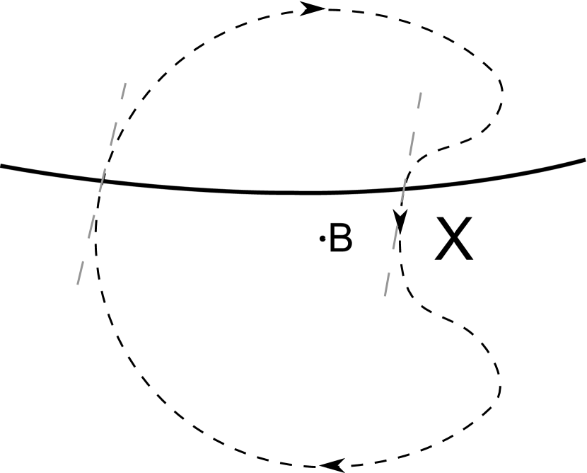
Figure 9: Example of a possible closed subbeam circulation loop (dashed line) around the magnetic pole (labelled $\bm{B}$) that would result in bi-drifting as observed by an observer whose line of sight samples a path indicated by the thick solid line. The rotational axis is somewhere above the magnetic axis (not shown). To observe bi-drifting, the tangents of the path at the intersection points (grey dashed lines) should be roughly parallel, unlike what would occur for a circular path. The X indicates the position of a possible obstruction responsible for the distorted circulation path.

Subbeam circulation configurations exist that meet the above requirements and could explain bi-drifting. An example of such a configuration is shown in Fig. 9. Drifting subpulses can be expected to be observed at all intersection points of the line of sight with the subbeam path where the two are not perpendicular to each other (otherwise longitude stationary on/off modulation would be observed without any drift). For a circular subbeam configuration the tangents to the subbeam path will be mirror-symmetric with respect to the meridian connecting the magnetic and rotation axis (vertical through the middle of the figure). This would mean that the same drift direction would be observed for two intersection points. Any path for which the two tangents are roughly parallel rather than mirror-symmetric would result in bi-drifting.

Any closed loop with the same tangents at the intersection points with the line of sight would result in identical observed drifting subpulse properties, hence Fig. 9 should be considered as an example of a possible configuration. The example in Fig. 9 might result from a distortion in the polar cap shape, forcing the subbeams to circulate around an obstruction (indicated with an X). For more realistic magnetic field line configurations the polar cap is indeed non-circular and a notch (Dyks et al., 2004) is expected. However, since both bi-drifters are likely to have relatively small magnetic inclinations, this effect cannot be expected to be particularly strong for these pulsars. Particularly large departures of an idealized dipolar field structure might be responsible for the deformed circulation path. The rarity of bi-drifters might indicate that there is a fine balance between having a large enough deformation without preventing regular circulation from being maintained. Possibly the mode changes are a consequence of the circulation failing at certain times. The observed drift rate as function of rotational phase, as can be quantified using the subpulse phase track, might in principle be used to quantify the shape of the circulation path and might be used to relate this to the required distortion in the magnetic field.

7 Summary and conclusions

A new set of software tools, available as a new open-source data-analysis project called PSRSALSA, were described and its power is illustrated by analysing the radio data of PSR B1839–04. In particular, the highly unusual phenomenon of bi-drifting was quantified in detail. Bi-drifting is the phenomenon that the drift direction of subpulses is different in different pulse profile components, which is very hard to explain theoretically.

A robust constraint on the magnetic inclination angle $\alpha$ was derived from archival radio polarization measurements after systematic consideration of the relevant uncertainties following the methodology described in Rookyard et al. (2015). PSR B1839–04 is likely to be relatively aligned ($\alpha$ is constrained to be smaller than $35\degr$). It is likely that the only other known bi-drifter, PSR J0815+0939, shares this property. Another similarity is that the wide profiles of both pulsars appear to be composed of four components.

WSRT observations revealed that two distinct emission modes operate in this pulsar, with the bi-drifting periodic subpulse modulation being present only during the Q mode. During the B mode, no regular drifting subpulses are observed, the pulse profile is more intense, and its components are closer to each other.

The bi-drifting in PSR B1839–04 is not clearly visible in a pulse stack. Nevertheless, utilising high-$S/N$ mode-separated data for the Q mode and sensitive analysis techniques, the existence of bi-drifting was convincingly demonstrated by exploiting the modulation power in the second harmonic observed in fluctuation analysis. Furthermore, bi-drifting was confirmed using $P_{3}$-folding. This is a completely independent method to visualise the subpulse modulation pattern by averaging over all pattern repetition periods $P_{3}$.

Three additional properties related to bi-drifting need to be explained by a viable model for subpulse modulation. First of all, while drifting subpulses are very common in the pulsar population, there are only two known examples of pulsars showing bi-drifting. This makes bi-drifting extremely rare. Secondly, for both bi-drifting pulsars $P_{3}$ is identical for all profile components. Thirdly, both bi-drifting pulsars are consistent with a symmetry such that all components in each half of the profile show the same drift sense, or no clear drift.

The modulation cycle of PSR B1839–04 is somewhat unstable, with significant variability in $P_{3}$ being detected. The variability in $P_{3}$ was shown to be identical in both components. Further analysis firmly established that the modulation pattern responsible for the bi-drifting is strictly phase-locked over a timescale of years. This means that if the modulation cycle is slow in one component, it is equally slow in the other such that the modulation patterns of both components stay in phase. The phase-locking is not disrupted by the mode changes, even though the modulation disappears during the B mode. This implies that a single physical origin is responsible for the modulation pattern observed in both components.

Phase-locking is critically difficult to explain by models. As a result, many ideas, some specifically proposed in the literature as a model for bi-drifting, were argued to be implausible. These include any model that requires oppositely circulating nested beamlet systems and any model invoking alias effects in the framework of nested beamlet systems or non-radial pulsations. Any model based on separate localised systems to explain the oppositely drifting subpulses requires communication between these systems to maintain synchronicity, effectively making it a single physical system. Phase-locking of subpulse modulation is reported for opposite magnetic poles of some pulsars, and the radiation of both poles could in principle be observed in a single on-pulse window if radiation is allowed to be directed towards the neutron star. However, such a scenario does not naturally lead to bi-drifting. The same is true for multiple projections of a single beamlet system, even if for instance magnetospheric refraction causes radiation to cross the magnetic axis.

We argued that within the framework of circulating beamlets scenarios exist that could explain drifting subpulses. They require subbeams to circulate around closed loops above the magnetic pole. For bi-drifting to occur, the loop must be distorted such that the tangents to the circulation path are roughly parallel rather than mirror-symmetric with respect to the meridian connecting the magnetic and rotation axis. This might reflect distortions in the magnetic field structure. It is possibly difficult to distort the circulation path enough for bi-drifting to occur without disrupting circulation altogether, which would explain the rarity of bi-drifting.