Social contagions on time-varying community networks

Abstract

Time-varying community structures widely exist in various real-world networks. However, the spreading dynamics on this kind of network has not been fully studied. To this end, we systematically study the effects of time-varying community structures on social contagions. We first propose a non-Markovian social contagion model on time-varying community networks based on the activity driven network model, in which an individual adopts a behavior if and only if the accumulated behavioral information it has ever received reaches a threshold. Then, we develop a mean-field theory to describe the proposed model. From theoretical analyses and numerical simulations, we find that behavior adoption in the social contagions exhibits a hierarchical feature, i.e., the behavior first quickly spreads in one of the communities, and then outbreaks in the other. Moreover, under different behavioral information transmission rates, the final behavior adoption proportion in the whole network versus the community strength shows one of the patterns, which are a monotone increasing pattern, a non-monotonic changing pattern, and a monotone decreasing pattern. An optimal community strength maximizing the final behavior adoption can be found in a suitable range of behavioral information transmission rate. Finally, for a given average degree, increasing the number of edges generated by active nodes is more beneficial to the social contagions than increasing the average activity potential.

I Introduction

The spreading dynamics is one of the hottest research topics in network science, which has attracted extensive attention from scholars in physics, mathematics, biology and other fields. The spreading dynamics aims to reveal the mechanisms in real spreading processes such as epidemic spreading, information spreading, behavior contagion and innovation diffusion, and further provides the theoretical support for forecasting and controlling these processes Pastor-Satorras2015 . The spreading dynamics can be divided into biological spreading and social contagion. The former focuses on the spreads of disease or virus on networks Pastor-Satorras2001 ; Newman2002a ; Gross2006 ; Small2007 , while the latter mainly studies contagions of information and behaviors on networks young2011 ; Centola2011 ; Adam2014 ; Gleeson2016 . The social reinforcement effect in social contagion is the essential difference between biological spreading and social contagion RMP2009 , which contains the idea that adoption behaviors of an individual often depends on his neighbors’ attitudes to the behavior watts2004 ; watts2005 ; centola2010 . For an individual, who has two friends having adopted a particular behavior before a given time and whose third friend newly adopts the behavior, his/her decision to adopt this behavior will take all the three friends into account.

For social contagions, researches focus on how social reinforcement effect influences the spreads of behaviors on static networks. The Markovian linear threshold model is a classic social contagion model to describe this reinforcement effect watts2002 . In the model, an individual that has not adopted a behavior becomes an adopter only when the number or proportion of its adopted neighbors exceeds a threshold. Watts found that the final behavior adoption proportion, following the increase of average degree, first grows continuously and then decreases discontinuously watts2002 . In fact, an individual’s decision to adopt a behavior not only depends on the current state of his/her neighbors, but also considers the behavioral information he has received. So the social reinforcement effect based on memory thus becomes an essential characteristic of social contagions. To describe the memory effect (i.e., non-Markovian effect), Wang et al. proposed a social contagion model based on non-redundant memory information, and found that the behavior adoption proportion versus the information transmission rate could exhibit a continuous growth or behavior as a discontinuous growth wangwei2015a ; Wang2016 . They also found that the individual’s limited contact capacity would reduce the final behavior adoption proportion Wangwei2015b .

The latest empirical studies showed that the connections among individuals in social networks vary with time, which can not be described by the static network. To this end, the conception of time-varying network (or temporal networks, dynamical networks) was proposed HolmePR . Perra et al. proposed an activity-driven network model to describe time-varying networks Perra2012 ; PerraPRL , which allows for an explicit representation of dynamical connectivity patterns. At each time step, every node becomes active or not according to its active potential. If a node becomes active, it will randomly connect to some nodes and form an instantaneous network structure. Spreading processes in activity-driven networks model show striking differences with respect to the well-known results obtained in quenched and annealed networks. Perra et al. found that the outbreak threshold of SIS model on an activity driven network is greater than that of the corresponding aggregated network Perra2012 . Liu et al. found that a disease spreads slower on activity driven networks than it does on the corresponding aggregated networks, and the invasion threshold on the former was hundreds of times greater than that of the latter LiuSY2013 . Holme et al. studied the threshold model on the time-varying networks based on empirical data, and found that time-varying network structures could enhance the final behavior adoption proportion holme2013 .

Community structures exist ubiquitously in real world networks Newman2002 ; Newman2006 , greatly affecting the spreading dynamics. For example, Liu et al. found that community structures make the epidemic spread more easily on static networks Liu2005 , and Ahn et al. found that there is an optimal community strength which can greatly promote the social contagions Ann2014 . Recent empirical studies showed that community structures also exists on time-varying networks HolmePR ; Mucha2012 . However, the effects of time-varying community structures on social contagion are little studied and full of challenges. On the one hand, the contacts on time-varying community networks change over time and do not happen continuously. On the other hand, the social reinforcement effects lead to the non-Markovian characteristic, making the existing theoretical method on static network difficult to accurately describe the spreading processes. In this paper, we systematically study the effects of time-varying community structures on social contagions. Firstly, we propose a non-Markovian social contagion model on time-varying community networks. Then, we develop a mean-field theory to quantify this contagion process and verify the accuracy of our predictions via extensive numerical simulations. With analyses and simulations, we find that behavior adoption exhibits a hierarchical feature: the behavior first spreads in one of the communities, and then outbreaks in the other. Moreover, under different transmission rates, the final behavior adoption proportion in the whole network versus community strength shows one of the following three patterns, which are an increasing pattern, a non-monotonic changing pattern, and a monotone decreasing pattern. An optimal community strength maximizing the final behavior adoption proportion can be found in a suitable transmission rate range. Moreover, we find that for a given average degree, adding the edges generated by active individuals is more beneficial to social contagions than increasing the average activity potential.

II Models

In order to study the effects of time-varying community networks on social contagions, we propose a non-Markovian social contagion model on activity-driven community network.

II.1 Activity-driven community network

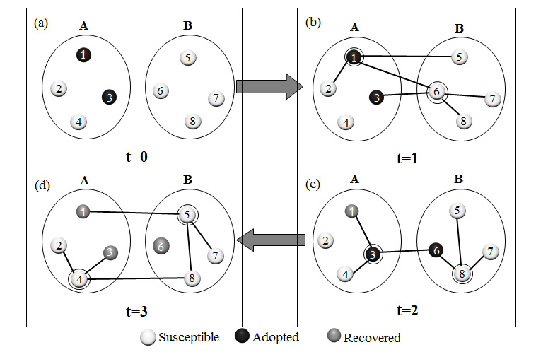
We generate a time-varying community network based on the activity driven network model Perra2012 . To simplify analysis, we suppose a network with $N$ nodes (representing individuals), consisting of two communities $A$ and $B$ with equal sizes. Initially, each node is assigned an equal activity potential $a$. The instantaneous network structure $G_{t}$ is generated as below: At time step $t$, each node is activated with probability $a$. If a node $v$ is activated, it will generate $m$ edges, each of which randomly connects to a node in the same community with probability $\mu$, called community strength, and connect to a node in the different community with probability $1-\mu$ [see Fig. 1]. Multiple edges and self-loops are not allowed. In order to form community structures, we set $\mu\in[0.5,1]$. Obviously, there will be less edges between the communities with the increase of $\mu$. For a small value of $\mu$, the community structure is not obvious. Note that when $\mu=0.5$, the probabilities of an edge connecting to the same and the different communities are equal, and the edges are connected completely randomly, thus the time-varying community structures disappear. When $\mu=1$, there is no edges between communities, leading to two totally isolated communities. At the end of time step $t$, we delete all the generated edges. Repeating the above process generates a time-varying community network.

Figure 1: (Color online) An illustration of social contagion model on activity-driven community network. The network is divided into two equal sized communities $A$ and $B$, each of which has 4 nodes. The circle around node reflects that node is active. (a) At $t=0$, randomly choose nodes 1 and 3 as seeds on community $A$, and the remaining nodes are susceptible. (b) At $t=1$, generate the instantaneous structure $G_{1}$, in which nodes 1 and 6 are activated with probability $a=0.25$ and generate $m=3$ edges. Every edge connects to nodes in the same community with probability $u=0.6$ and with probability $1-u=0.4$ to the other community. Adopted nodes 1 and 3 transmit the behavioral information to susceptible neighbors with $\lambda=0.8$. Node 6 receives 2 pieces of information successfully, and reaches the adoption threshold $\pi=2$, thus it becomes adopted. Nodes 1 and 3 become recovered with $\gamma=0.1$. Delete all edges generated at this time step. (c) At $t=2$, nodes 3 and 8 are active and form the instantaneous structure $G_{2}$. Node 3 transmits the behavioral information to node 8 successfully, and nodes 3 and 6 become recovered. (d) At $t=3$, nodes 4 and 5 are activated in the instantaneous structure $G_{3}$. The contagion process terminates since all adopted nodes become recovered.

II.2 Social contagion model

We propose a non-Markovian social contagion model, called susceptible-adopted-recovered (SAR) model, to describe behavior spreading on time-varying community networks wangwei2015a ; Shu2016 . At a given time step, a node can be in one of the three states: susceptible, adopted, and recovered. In the susceptible state, a node has not adopted the behavior and is willing to receive behavioral information from its neighbors who has adopted the behavior. In the adopted state, a node who has adopted the behavior and is keen to spread the behavioral information to its neighbors. In the recovered state, a node will lose its interest to the behavior and no longer anticipate the spreading process. Each node holds a static equal adoption threshold $\pi$, which reflects the wills of this node to adopt the behavior. Each node has variable $\chi_{i}$ to count how many pieces of behavioral information it has received.

At the beginning, a proportion $\rho_{0}$ of nodes are randomly chosen as seeds (initial adopters), while the remaining nodes are susceptible. We use synchronous updating method to update nodes’ state wangwei2015a . At each time step, we first generate an instantaneous structure $G_{t}$ according to the method described in Sec. II.1. Then, the behavior spreads on network $G_{t}$ as follows. Every adopted node $v$ transmits the behavioral information to each susceptible neighbor $u$ with probability $\lambda$. If $u$ receives the information successfully, his corresponding accumulated information counter $\chi_{u}$ will add one. If $\chi_{u}$ reaches or exceeds the adoption threshold $\pi$, the node $u$ becomes adopted state. The dynamics of social contagion is a non-Markovian stochastic process. For the case of $\pi=1$, the model becomes memoryless, thus we only discuss the situations when $\pi>1$. At the same time step, the adopted nodes become recovered with probability $\gamma$. The contagion process terminates when all adopted nodes become recovered. In this model, the probabilities $\lambda$ and $\gamma$ can be interpreted as transmission rate and recover rate respectively, for they are expected to equal to the proportion of information successfully arrived and nodes turning into recover state at each time step. An illustration of our social contagion model on time-varying community network is given in Fig. 1.

III Theory

In this section, we develop a mean-field approximation theory to quantitatively describe the non-Markovian social contagions on time-varying community network. We denote the proportion of susceptible nodes who have received $r$ pieces of behavioral information in community $A$ and community $B$ at time step $t$ as $S_{A}(r,t)$ and $S_{B}(r,t)$ (denominator is $N/2$), respectively. We respectively use $\rho_{A}(t)$ and $\rho_{B}(t)$ to denote the proportion of adopted nodes in communities $A$ and $B$, and $R_{A}(t)$ and $R_{B}(t)$ to denote the proportion of recovered nodes at time step $t$. When $t\rightarrow\infty$, all adopted nodes become recovered. We denote the final proportion of nodes in the recovered state in communities $A$ and $B$ as $R_{A}(\infty)$ and $R_{B}(\infty)$, respectively. The final behavior adoption proportion in the whole network is then $R(\infty)=[R_{A}(\infty)+R_{B}(\infty)]/2$, since communities $A$ and $B$ have the same size.

Due to the symmetry of the two communities, we only introduce the theoretical analyses on community $A$ detailedly, and the results on community $B$ can be derived by simply exchanging the index $A$ and $B$. At time step $t$, a node $v_{A}$ forms its $k$ edges in the instantaneous structure $G_{t}$ in two different ways: (i) edges generated by $v_{A}$ itself, denoted as its out-going degree $k_{o}$; (ii) edges generated by other active nodes in the network connecting to $v_{A}$, denoted as its in-coming degree $k_{i}$. As a result, the degrees of node $v_{A}$ is $k=k_{i}+k_{o}$. One can assume that the degrees of active nodes are equal, and the degree of inactive nodes are also the same. According to the formation of the time-varying community networks described in Sec. II, node $v_{A}$ generates $m$ edges to connect to other nodes when it is active, thus $k_{o}=m$. At the same time, other active nodes in the network generate edges and try to connect to $v_{A}$. For there are expected $am(N-1)$ edges to be remained on $G_{t}$, node $v_{A}$ will get $k_{i}=(N-1)am/N\approx ma$ connections since the communities $A$ and $B$ are symmetric. Thus, we obtain the expected degree of active nodes as $k=m+ma$ Lixiang2014 . When $v_{A}$ is inactive, $k_{o}=0$ while $k_{i}$ remains the same, thus $k=k_{i}=ma$. For active nodes, each of its edges connects to a node in the same community with probability $\mu$ and connects to the different community with probability $1-\mu$. The probability that node $v_{A}$ connecting to $n$ nodes in community $A$ when it is active can thus be written as

$$\omega^{AA}_{Active}(n)=\binom{m+ma}{n}\mu^{n}(1-\mu)^{m+ma-n}.$$ (1)

Similarly, the probability that node $v_{A}$ connecting to $n$ nodes in community $B$ is given by

$$\omega^{AB}_{Active}(n)=\binom{m+ma}{n}(1-\mu)^{n}\mu^{m+ma-n}.$$ (2)

If node $v_{A}$ is inactive, the probability that $v_{A}$ has $n$ edges connecting to nodes in community $A$ or $B$ are

$$\omega^{AA}_{Inactive}(n)=\binom{ma}{n}\mu^{n}(1-\mu)^{ma-n}$$ (3)

and

$$\omega^{AB}_{Inactive}(n)=\binom{ma}{n}(1-\mu)^{n}\mu^{ma-n},$$ (4)

respectively.

On the instantaneous structure $G_{t}$, the probability that a node $v_{A}$ in community $A$ with degree $k=k_{A}$ has $x_{A}$ adopted neighbors in community $A$ is

$$\xi_{AA}(k_{AA},x_{A},t)=\binom{k_{AA}}{x_{A}}[\rho_{A}(t)]^{x_{A}}[1-\rho_{A}(t)]^{k_{AA}-x_{A}},$$ (5)

where $k_{AA}$ denotes the number of neighbors of node $v_{A}$ in community $A$. Similarly, the probability that $v_{A}$ has $x_{B}$ adopted neighbors in community $B$ can be written as

$$\xi_{AB}(k_{AB},x_{B},t)=\binom{k_{AB}}{x_{B}}[\rho_{B}(t)]^{x_{B}}[1-\rho_{B}(t)]^{k_{AB}-x_{B}},$$ (6)

where $k_{AB}$ is the number of neighbors of $v_{A}$ in community $B$ and $k_{AB}=k_{A}-k_{AA}$.

We separately consider the situations that $v_{A}$ is active or inactive at time step $t$. For the former situation, combining Eqs. (1) and (5)-(6), the probability that the active $v_{A}$ connects to $n$ adopted nodes is

$$\begin{split}\theta^{A}_{Active}(n,t)&=\sum^{m+ma}_{i=0}\omega^{AA}_{Active}(i)\sum^{{\rm min}(n,i)}_{j=0}[\xi_{AA}(i,j,t)\\ &\times\xi_{AB}(m+ma-i,n-j,t)],\end{split}$$ (7)

where we use ${\rm min}(x,y)$, meaning the minimum value of $x$ and $y$, to avoid the situations that $j$ exceeds $i$. When node $v_{A}$ is inactive at time step $t$, the probability that $v_{A}$ connects to $n$ adopted nodes can be obtained by combining Eqs. (3) and (5)-(6),

$$\begin{split}\theta^{A}_{Inactive}(n,t)&=\sum^{ma}_{i=0}\omega^{AA}_{Inactive}(i)\sum^{{\rm min}(n,i)}_{j=0}[\xi_{AA}(i,j,t)\\ &\times\xi_{AB}(ma-i,n-j,t)].\end{split}$$ (8)

Summarize the two situations and combining Eqs. (7)-(8), the probability that $v_{A}$ connects to $n$ adopted individuals on $G_{t}$ is given by

$$\theta_{A}(n,t)=a\theta^{A}_{Active}(n,t)+(1-a)\theta^{A}_{Inactive}(n,t).$$ (9)

Then we focus on the time evolution of the density of nodes in each state. According to the social contagion model, when a susceptible node $v_{A}$ has $n$ adopted neighbors at time step $t$, the probability that it receives at least one piece of behavioral information from its neighbors is

$$\psi_{A}(t)=\sum^{m+ma}_{n=1}\theta_{A}(n,t)[1-(1-\lambda)^{n}].$$ (10)

The probability that $v_{A}$ receives $i\geq 1$ pieces of behavioral information can be expressed as

$$\phi_{A}(i,t)=\sum^{m+ma}_{n=i}\theta_{A}(n,t)\binom{n}{i}\lambda^{i}(1-\lambda)^{n-i}.$$ (11)

Obviously, Eq. (10) can be derived by Eq. (11) as

$$\psi_{A}(t)=\sum^{m+ma}_{i=1}\phi_{A}(i,t).$$ (12)

Then the time evolution of the contagion process can be described by a developed mean-field method. For those nodes who have not received any behavioral information at time step $t$, denoted as $S_{A}(0,t)$, they change into other states when receiving at least one piece of behavioral information, yielding

$$\frac{dS_{A}(0,t)}{dt}=-S_{A}(0,t)\psi_{A}(t).$$ (13)

When $1\leq r<\pi$, the increase of $S_{A}(r,t)$ comes from these nodes who have only received less than $r$ pieces of behavioral information, that is $S_{A}(q,t)$ ($0\leq q<r$), change into $S_{A}(r,t)$ after receiving $r-q$ pieces of behavioral information, with probability $\sum^{r-1}_{q=0}S_{A}(q,t)\phi_{A}(r-q,t)$. At the same time, $S_{A}(r,t)$ decreases after those nodes receive at least one information and then turns to other states, with the probability $S_{A}(r,t)\psi_{A}(t)$. Thus, the evolution equation of $S_{A}(r,t)$ can be written as

$$\frac{dS_{A}(r,t)}{dt}=\sum^{r-1}_{q=0}S_{A}(q,t)\phi_{A}(r-q,t)-S_{A}(r,t)\psi_{A}(t).$$ (14)

Similarly, the increase of adopted nodes results from the state change of susceptible nodes who have received information being equal or over the threshold $\pi$, with probability $\sum^{\pi-1}_{q=0}S_{A}(q,t)[\psi_{A}(t)-\sum^{\pi-1-q}_{i=1}\phi_{A}(i,t)]$, and the decrease owes to the recovering of themselves, with probability $\gamma\rho_{A}(t)$. Thus the evolution of the densities of adopted and recovered nodes can be written as

$$\frac{d\rho_{A}(t)}{dt}=\sum^{\pi-1}_{q=0}S_{A}(q,t)[\psi_{A}(t)-\sum^{\pi-1-q}_{i=1}\phi_{A}(i,t)]-\gamma\rho_{A}(t)$$ (15)

and

$$\frac{dR_{A}(t)}{dt}=\gamma\rho_{A}(t),$$ (16)

respectively.

Now, Eqs. (13)-(16) form a complete description of the social contagion process, allowing us to compute the proportion of nodes in any state in community $A$ at any time step. By transferring our knowledge to community $B$ i.e., exchanging the positions of index $A$ and $B$, the time evolutions in community $B$ and in the whole network are also available. When all adopted nodes become recovered, we count the final behavior adoption proportion $R(\infty)=[R_{A}(\infty)+R_{B}(\infty)]/2$.

The outbreak threshold of social contagion $\lambda_{c}$ is a crucial parameter. When the information transmission rate $\lambda$ is greater than $\lambda_{c}$, a finite fraction of nodes adopt the behavior. When $\lambda\leq\lambda_{c}$, there is only a vanishingly small fraction of nodes adopting the behavior. Initially, there are a few nodes in the adopted state, thus $\rho_{A}(0)\rightarrow 0$, $\rho_{B}(0)\rightarrow 0$, $R_{A}(0)\rightarrow 0$ and $R_{B}(0)\rightarrow 0$. Previous studies indicate that the behavior can outbreak over the network, if and only if the proportion of adopted individuals can exponentially grow at initial time WangWeiSR ; NewmanBook . Thus, one expects to obtain $\lambda_{c}$ by stability analysis method. Unfortunately, this method is useless to our model because of the memory effect. On the one hand, a vanishingly small fraction of initial adopters can not lead to the quick growth of behavior at initial time in our model, for the susceptible nodes cannot immediately accumulate the information memory to reach or exceed the adoption threshold $\pi$ when the initial adopters are very rare. On the other hand, the appearance of nonlinearity in the system makes the linearization method near the stability point ineffective Radicchi2015 . Therefore, the outbreak threshold can not be obtained by the existing method. To get the outbreak threshold, further researches are needed.

IV Simulation Results

Based on the proposed model, we performed extensive simulations to investigate the social contagions on time-varying community networks. In simulations, the size of network, recover probability and adoption threshold are set to be $N=10,000$, $\gamma=0.1$ and $\pi=3$, respectively. At the beginning, a proportion $\rho_{0}=0.06$ of nodes in Community $A$ are randomly chosen as seeds, while the remaining nodes are susceptible. The simulation results of the final adoption proportion $R_{A}(\infty)$, $R_{B}(\infty)$ and $R(\infty)$ are obtained by averaging the results over $2000$ independent realizations. The theoretical values of $R_{A}(\infty)$, $R_{B}(\infty)$ and $R(\infty)$ are given by solving Eqs. (13)-(16). We separately discuss the effects of community structure and the time-varying structure on the social contagions.

IV.1 Effects of community structure

Figure 2: (Color online) The final behavior adoption proportion $R_{A}(\infty)$, $R_{B}(\infty)$ and $R(\infty)$ versus information transmission probability $\lambda$ under different community strengths. (a) $\mu=0.5$, (b) $\mu=0.9$, (c) $\mu=0.95$, and (d) $\mu=0.97$. The solid line (circles), dotted line (squares) and dotted line (diamonds) represent the theoretical predictions (simulation results) of $R_{A}(\infty)$, $R_{B}(\infty)$ and $R(\infty)$. The insets of (b) and (d) show simulation results of $\rho_{A}(t)$, $\rho_{B}(t)$ and $\rho(t)$ versus $t$. Other parameters are set to be $N=10,000$, $\rho_{0}=0.03$, $a=0.2$, $m=5$, $\gamma=0.1$ and $\pi=3$, respectively.

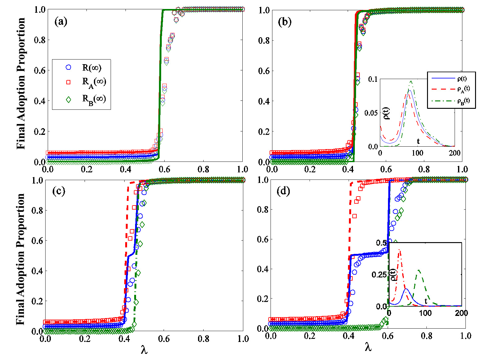
We firstly study the growths of $R_{A}(\infty)$, $R_{B}(\infty)$ and $R(\infty)$ versus $\lambda$ under different $\mu$ in Fig. 2, which show different growth patterns. For relatively small values $\mu=0.5$ and $0.9$, nodes in community $A$ and community $B$ adopt the behavior at almost the same time [see Figs. 2(a)-(b)]. That is because the community structure is not obvious when $\mu$ is relatively small, and the adopted nodes are able to transmit the behavioral information to nodes in the whole network. For relatively large values of $\mu=0.95$ and $0.97$, the behavior adoption exhibits a hierarchical feature: nodes in community $A$ first adopt the behavior, and then nodes in community $B$ adopt the behavior with the increase of $\lambda$ [Figs. 2(c)-(d)]. When $\mu$ is relatively large, nodes tend to transmit information to those nodes in the same community, which adds difficulty to transmit the information to community $B$. The insets of Figs. 2 (b) and (d) show the corresponding growth patterns of $\rho_{A}(\infty)$, $\rho_{B}(\infty)$ and $\rho(\infty)$ versus time $t$, which confirms the hierarchical feature shown in the behavior adoption process. The theoretical predictions agree well with the simulation results, giving a quantitative description of the above phenomena. The deviations between the theoretical predictions and the simulation results are caused by the dynamical correlations among the states of the neighbors and finite-size network effects Reche2011 ; Cui2014 .

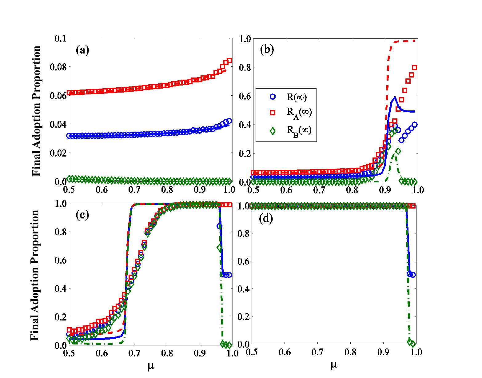
Figure 3 exhibits the growths of $R_{A}(\infty)$, $R_{B}(\infty)$ and $R(\infty)$ versus $\mu$ under different $\lambda$. Three different growth patterns can be observed. For small values of $\lambda$ in Fig. 3(a), $R(\infty)$, $R_{A}(\infty)$ and $R_{B}(\infty)$ monotonically increase with growing $\mu$. With the increase of $\lambda$, shown in Figs. 3 (b)-(c), $R_{A}(\infty)$ increases with $\mu$ monotonically, while $R_{B}(\infty)$ and $R(\infty)$ first increase and then decrease, which indicates the existence of optimal community strength promoting the behavior adoption. The optimal contagion phenomena can be explained as below: There are more edges in the community for a larger $\mu$, which promotes the behavior spreading on community $A$. Meanwhile, the amount of bridge edges between communities decreases with growing $\mu$. If $\mu$ is large enough, the global behavior adoption will be inhibited, which leads to the decrease of $R_{B}(\infty)$ and $R(\infty)$. When $\lambda$ is very large, nodes in both communities adopt the behavior easily [see Fig. 3(d)]. For any given $\mu$, the $R_{A}(\infty)$ can always reach a remarkable value. Only when $\lambda$ is great enough, the two communities tend to be isolated and the global behavior adoption is suppressed, thus $R_{B}(\infty)$ and $R(\infty)$ begin to decrease.

Figure 3: (Color online) The final behavior adoption proportion $R_{A}(\infty)$, $R_{B}(\infty)$ and $R(\infty)$ versus community strength $\mu$ under different information transmission rates (a) $\lambda=0.35$, (b) $\lambda=0.4$3, (c) $\lambda=0.55$ and (d) $\lambda=0.7$. The solid line (circles), dotted line (squares) and dotted line (diamonds) represent the theoretical values (simulation values) of $R_{A}(\infty)$, $R_{B}(\infty)$ and $R(\infty)$, respectively. Other parameters are set to be $N=10,000$, $\rho_{0}=0.03$, $a=0.2$, $m=5$, $\gamma=0.1$ and $\pi=3$, respectively.

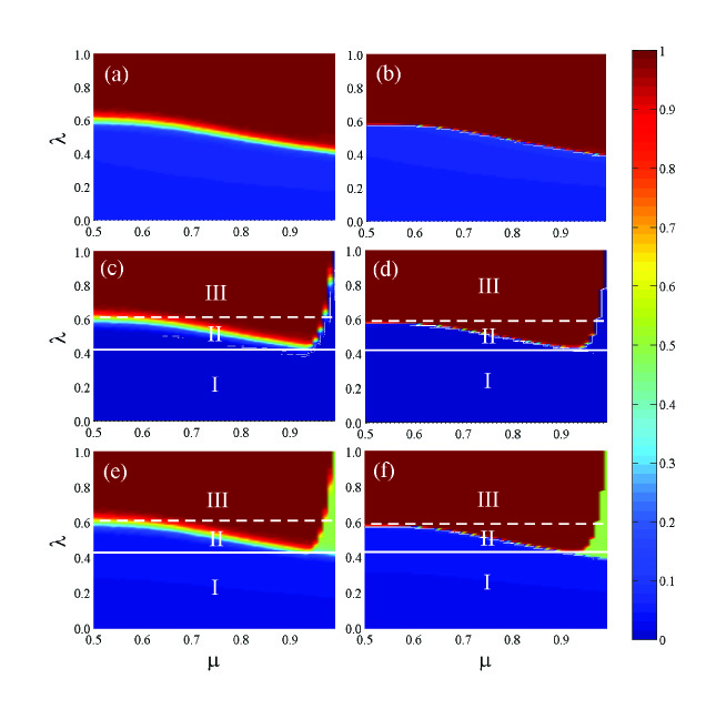
We show the effects of $\lambda$ and $\mu$ on $R_{A}(\infty)$, $R_{B}(\infty)$ and $R(\infty)$ in Fig. 4. According to the growth patterns of $R(\infty)$, $R_{A}(\infty)$ and $R_{B}(\infty)$ versus $\mu$ in Figs. 4(c)-(f), $\mu$-$\lambda$ plane can be divided into three regions: (I) monotonically increasing region, (II) non-monotonically changing region and (III) monotonically decreasing region. As $R_{A}(\infty)$ increases monotonically with $\mu$, Figs.4(a)-(b) only exist region I. Due to the effect of time-varying community structures, Figs. 4(c)-(f) exhibits three different regions, which means that there exists an optimal community strength in a certain range of $\lambda$, making the values of $R_{B}(\infty)$ and $R(\infty)$ reach the maximum values. The theoretical results in Fig. 4(b),(d),(f) can well predict the simulation results in Figs. 4(a),(c),(e).

Figure 4: (Color online) The final behavior adoption proportion $R_{A}(\infty)$, $R_{B}(\infty)$ and $R(\infty)$ versus community strength $\mu$ and information transmission rate $\lambda$. Color-coded values show simulation results in (a) $R_{A}(\infty)$ ,(c) $R_{B}(\infty)$ and (e) $R(\infty)$, and theoretical predictions in (b) $R_{A}(\infty)$, (d) $R_{B}(\infty)$ and (f) $R(\infty)$. Other parameters are set to be $N=10,000$, $\rho_{0}=0.03$, $a=0.2$, $m=5$, $\gamma=0.1$ and $\pi=3$, respectively.

IV.2 Effects of time-varying structure

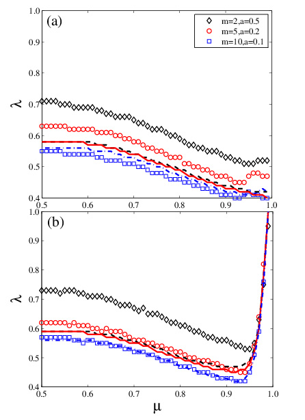
In Fig. 5, we investigate the effect of time-varying structure on social contagions. According to the description of the time-varying community structures, the average degree of $G_{t}$ is $\langle k\rangle=2ma$ at time step $t$, which allows us to compare the relative importance of time-varying structure parameters $m$ and $a$ on the social contagions. We keep the rest of parameters the same as Fig. 2 and fix the average degree $\langle k\rangle=2$, then adjust the values of $m$ and $a$. For a given $R(\infty)$ and $\mu$, we record the corresponding values of $\lambda$, i.e., getting the contours of different $R(\infty)$ in the $\lambda$-$\mu$ plane. If the importance of $m$ and $a$ are equal, their influences on social contagions will counteract each other, and the simulation results will remain almost the same. However, we find that the information transmission rate $\lambda$ needed to reach the specified $R(\infty)$ decreases with the increase of $m/a$, which implies that, compared to adjusting the the value of $a$, adjusting $m$ is more beneficial to social contagions. We can understand the phenomenon in the following way: Increasing the value of $m/a$ means decreasing the number of active nodes and increasing the average degree of active nodes, which leads to emerge of active nodes with high degree. When active nodes have high degree, they will have high probability to touch enough adopted nodes and become adopted at one time step, thus these contacts are effective. On the contrary, small $m/a$ will result in low degree of active nodes in instantaneous structure. These active nodes will not receive enough information at one time step, and wait for another round of activating, which is not so effective. Though active nodes existing at one step are few because of small $a$, high degree situation can be more efficiently, and eventually reach the assigned $R(\infty)$ more quickly. For other average degree, such as $\langle k\rangle=0.2,1,3$, the same phenomena can be observed. Our theoretical method also displays the same phonomania about the effects of $m/a$ in Fig. 5.

Figure 5: (Color online) The behavioral information transmission rate $\lambda$ versus community strength $\mu$ for a given behavior adoption proportion (a) $R(\infty)=0.4$ and (b) $R(\infty)=0.7$. The dotted line (diamonds), solid (circles) and dotted line (squares) denote the theoretical values (simulated values) of $m=2$, $a=0.5$, $m=5$, $a=0.2$ and $m=10$, a=0.1, respectively Other parameters are set to be $N=10,000$, $\rho_{0}=0.03$, $a=0.2$, $m=5$, $\gamma=0.1$ and $\pi=3$, respectively.

V Discussion

In this paper, we studied the effects of time-varying community structures on social contagions. We first proposed a non-Markovian social contagion model on time-varying community network, and then develop a mean-field theory to quantitatively describe the proposed model. Through theoretical analyses and extensive numerical simulations, we found that behavior adoption exhibits a hierarchical feature. The behavior first spreads in one of the communities, and then outbreaks in the other. Moreover, under different behavioral information transmission rates, the final behavior adoption proportion in the whole network versus the community strength can show one of the different patterns, such as, a monotone increasing pattern, a non-monotonic changing pattern, and a monotone decreasing pattern. In non-monotonic changing pattern, we found an optimal community strength under which the final behavior adoption proportion reaches its maximum value. Finally, we discovered that for a given average degree, increasing the number of edges generated by active nodes is more beneficial to the social contagions than increasing the average activity potential. Our proposed theory predicted the phenomena on social contagion well.

We qualitatively and quantitatively studied how time-varying community structures affect the social contagions. First, we described timeliness of the edges by using the time-varying network model, compensating the lack of static network research methods. In addition, the proposed non-Markovian social contagion model described social contagion process on time-varying community network more accurately than Markovian models. Furthermore, our developed theory predicted qualitatively the occurrence of various phenomena in simulations. In conclusion, this work helps us in better understanding, predicting and controlling the social contagions on social networks. The effects of social contagions on epidemic spreading and the relationship between time-varying networks and multilayer networks are worthy of future study Ruan2012 ; YangHX2015 ; Arenas2013 ; Arenas2014 .