Support Vector Algorithms for Optimizing the
Partial Area Under the ROC Curve

Harikrishna Narasimhan111This work was done when the author was a PhD student at the Indian Institute of Science, Bangalore.
John A. Paulson School of Engineering and Applied Sciences, Harvard University
Cambridge, MA 02138, USA
Email: hnarasimhan@seas.harvard.edu
   Shivani Agarwal
Radcliffe Institute for Advanced Study, Harvard University
Cambridge, MA 02138, USA
Department of Computer Science and Automation, Indian Institute of Science
Bangalore 560012, INDIA
Email: shivani@csa.iisc.ernet.in
Abstract

The area under the ROC curve (AUC) is a widely used performance measure in machine learning. Increasingly, however, in several applications, ranging from ranking to biometric screening to medicine, performance is measured not in terms of the full area under the ROC curve, but in terms of the partial area under the ROC curve between two false positive rates. In this paper, we develop support vector algorithms for directly optimizing the partial AUC between any two false positive rates. Our methods are based on minimizing a suitable proxy or surrogate objective for the partial AUC error. In the case of the full AUC, one can readily construct and optimize convex surrogates by expressing the performance measure as a summation of pairwise terms. The partial AUC, on the other hand, does not admit such a simple decomposable structure, making it more challenging to design and optimize (tight) convex surrogates for this measure.

Our approach builds on the structural SVM framework of Joachims (2005) to design convex surrogates for partial AUC, and solves the resulting optimization problem using a cutting plane solver. Unlike the full AUC, where the combinatorial optimization needed in each iteration of the cutting plane solver can be decomposed and solved efficiently, the corresponding problem for the partial AUC is harder to decompose. One of our main contributions is a polynomial time algorithm for solving the combinatorial optimization problem associated with partial AUC. We also develop an approach for optimizing a tighter non-convex hinge loss based surrogate for the partial AUC using difference-of-convex programming. Our experiments on a variety of real-world and benchmark tasks confirm the efficacy of the proposed methods.

footnotetext:  
Parts of this paper were presented at the 30th International Conference on Machine Learning, 2013 [29] and at the 19th ACM SIGKDD Conference on Knowledge Discovery and Data Mining, 2013 [30].

1 Introduction

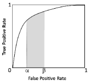
The receiver operating characteristic (ROC) curve plays an important role as an evaluation tool in machine learning and data science. In particular, the area under the ROC curve (AUC) is widely used to summarize the performance of a scoring function in binary classification problems, and is often a performance measure of interest in bipartite ranking [8, 3]. Increasingly, however, in several applications, the performance measure of interest is not the full area under the ROC curve, but instead, the partial area under the ROC curve between two specified false positive rates (FPRs) (see Figure 1). For example, in ranking applications where accuracy at the top is critical, one is often interested in the left-most part of the ROC curve [38, 1, 35]; this corresponds to maximizing partial AUC in a false positive range of the form [0,β]0𝛽[0,\beta]. In biometric screening, where false positives are intolerable, one is again interested in maximizing the partial AUC in a false positive range [0,β]0𝛽[0,\beta] for some suitably small β𝛽\beta. In the KDD Cup 2008 challenge on breast cancer detection, performance was measured in terms of the partial AUC in a specific false positive range [α,β]𝛼𝛽[\alpha,\beta] deemed clinically relevant [36].222More specifically, the KDD Cup 2008 challenge used the partial area under the free-response operating characteristic curve, where a scaled version of usual FPR is used.

In this paper, we develop support vector machine (SVM) based algorithms for directly optimizing the partial AUC between any two false positive rates α𝛼\alpha and β𝛽\beta. Our methods are based on minimizing a suitable proxy or surrogate objective for the partial AUC error. In the case of the full AUC, where the evaluation measure can be expressed as a summation of pairwise indicator terms, one can readily construct and optimize surrogates by exploiting this structure. The partial AUC, on the other hand, does not admit such a decomposable structure, as the set of negative instances associated with the specified false positive range can be different for different scoring models; as a result, it becomes more challenging to design and optimize convex surrogates for this measure.
Refer to caption
Figure 1: Partial AUC in false positive range [α,β]𝛼𝛽[\alpha,\beta].

For instance, a popular approach for constructing convex surrogates for the full AUC is to replace the indicator terms in its definition with a suitable pairwise convex loss such as the pairwise hinge loss; in fact, there are several efficient methods available to solve the resulting optimization problem [14, 17, 18]. This is not the case with the more complex partial AUC measure; here, a surrogate constructed by replacing the indicators with the pairwise hinge loss is non-convex in general. Even in the special case of FPR intervals of the form [0,β]0𝛽[0,\beta], where the hinge loss based surrogate turns out to be convex, solving the resulting optimization problem is not straightforward.

In our approach, we construct and optimize convex surrogates on the partial AUC by building on the structural SVM formulation of Joachims (2005) developed for general complex performance measures [18]. It is known that for the full AUC, this formulation recovers the corresponding hinge surrogate [19]. On the other hand, a direct application of this framework to the partial AUC results in a loose approximation to the performance measure (in a sense that we will elaborate in later sections). Instead, we first rewrite the evaluation measure as a maximum of a certain term over subsets of negative instances, and leverage the structural SVM setup to construct a convex approximation to the inner term. This yields a tighter surrogate, which for the special case of partial AUC in the [0,β]0𝛽[0,\beta] range, is equivalent to the hinge surrogate obtained by replacing the indicators with the pairwise hinge loss; for general FPR intervals [α,β]𝛼𝛽[\alpha,\beta], the surrogate obtained can be seen as a convex relaxation to the (non-convex) hinge surrogate.

We make use of the cutting plane method to optimize the proposed structural SVM surrogates. Each iteration of this solver requires a combinatorial search over subsets of instances and over binary matrices (representing relative orderings of positive and negative training instances) to find the currently most violated constraint. In the case of the full AUC (where the optimization is only over binary matrices), this problem decomposes neatly into one where each matrix entry can be chosen independently [18]. Unfortunately, for the partial AUC, a straightforward decomposition is not possible, again because the negative instances involved in the relevant false positive range can be different for different orderings of instances.

One of our main contributions in this paper is a polynomial time algorithm for solving the corresponding combinatorial optimization within the cutting plane method for the partial AUC, by breaking down the problem into smaller tractable ones. When the specified false positive range is of the form [0,β]0𝛽[0,\beta], we show that after fixing the optimal subset of negatives to the top ranked negatives, one can still optimize the individual entries of the ordering matrix separately. For the general case [α,β]𝛼𝛽[\alpha,\beta], we require to further formulate an equivalent optimization problem over a restricted search space, where each row of the matrix can be optimized separately – and efficiently.

While the use of convex surrogates in the above approach allows for efficient optimization and guarantees convergence to the global surrogate optimum, it turns out that for the partial AUC in a general FPR interval [α,β]𝛼𝛽[\alpha,\beta], the previous non-convex hinge surrogate (obtained by replacing the indicators with the pairwise hinge loss) is a tighter approximation to the original evaluation measure. Hence, as a next step, we also develop a method for directly optimizing this non-convex surrogate using a popular non-convex optimization technique based on difference-of-convex (DC) programming; here we exploit the fact that the partial AUC in [α,β]𝛼𝛽[\alpha,\beta] can be written as a difference of (scaled) partial AUC values in [0,β]0𝛽[0,\beta] and [0,α]0𝛼[0,\alpha].

We evaluate the proposed methods on a variety of real-world applications where partial AUC is an evaluation measure of interest and on benchmark data sets. We find that in most cases, the proposed methods yield better partial AUC performance compared to an approach for optimizing the full AUC, thus confirming the focus of our methods on a select false positive range of the ROC curve. Our methods are also competitive with existing algorithms for optimizing partial AUC. For partial AUC in [α,β]𝛼𝛽[\alpha,\beta], we find that in some settings, the proposed DC programming method for optimizing the non-convex hinge surrogate (despite having the risk of getting stuck at a locally optimal solution) performs better than the structural SVM method, though overall there is no clear winner.

1.1 Related Work

There has been much work on developing algorithms to optimize the full AUC, mostly in the context of ranking [14, 17, 13, 5, 18]. There has also been interest in the ranking literature in optimizing measures focusing on the left end of the ROC curve, corresponding to maximizing accuracy at the top of the list [38]; in particular, the Infinite Push ranking algorithm [1, 35] can be viewed as maximizing the partial AUC in the range [0,1n]01𝑛\big{[}0,\frac{1}{n}\big{]}, where n𝑛n is the number of negative training examples.

While the AUC is widely used in practice, increasingly, the partial AUC is being preferred as an evaluation measure in several applications in bioinformatics and medical diagnosis [33, 34, 36, 16], and more recently even in domains like computer vision [31, 32], personalized medicine [25], and demand forecasting [39]. The problem of optimizing the partial AUC in false positive ranges of the form [0,β]0𝛽[0,\beta] has received some attention primarily in the bioinformatics and biometrics literature [33, 11, 44, 37, 15]; however in most cases, the algorithms developed are heuristic in nature. The asymmetric SVM algorithm of [45] also aims to maximize the partial AUC in a range [0,β]0𝛽[0,\beta] by using a variant of one-class SVM; but the optimization objective used does not directly approximate the partial AUC in the specified range, but instead seeks to indirectly promote good partial AUC performance through a fine-grained parameter tuning procedure. There has also been some work on optimizing the partial AUC in general false positive ranges of the form [α,β]𝛼𝛽[\alpha,\beta] including the boosting-based algorithms pAUCBoost [22] and pU-AUCBoost [40].

Support vector algorithms have been extensively used in practice for various supervised learning tasks, with both standard and complex performance measures [9, 10, 6, 17, 41]. The proposed methods are most closely related to the structural SVM framework of Joachims for optimizing the full AUC [18]. To our knowledge, ours is the first work to develop principled support vector methods that can directly optimize the partial AUC in an arbitrary false positive range [α,β]𝛼𝛽[\alpha,\beta].

1.2 Paper organization.

We begin with the problem setting in Section 2, along with background material on the previous structural SVM framework for full AUC maximization. In Section 3, we consider two initial surrogates for the partial AUC, one based on the pairwise hinge loss and the other based on a naïve application of the structural SVM formulation, and point out drawbacks in each case. We then present a tight convex surrogate for the special case of FPR range [0,β]0𝛽[0,\beta] in Section 4 and for the general case of [α,β]𝛼𝛽[\alpha,\beta] intervals in Section 5, along with cutting plane solvers for solving the resulting optimization problem. Subsequently in Section 6, we also describe a DC programming approach for directly optimizing the non-convex hinge surrogate for partial AUC in [α,β]𝛼𝛽[\alpha,\beta]. We provide a generalization bound for the partial AUC in Section 7, and present our experimental results on real-world and benchmark tasks in Section 8.  

2 Preliminaries and Background

2.1 Problem Setting

Let X𝑋X be an instance space and 𝒟+subscript𝒟{\mathcal{D}}_{+} and 𝒟subscript𝒟{\mathcal{D}}_{-} be probability distributions over positive and negative instances in X𝑋X. We are given a training sample S=(S+,S)𝑆subscript𝑆subscript𝑆S=(S_{+},S_{-}) containing m𝑚m positive instances S+=(x1+,,xm+)Xmsubscript𝑆subscriptsuperscript𝑥1subscriptsuperscript𝑥𝑚superscript𝑋𝑚S_{+}=(x^{+}_{1},\ldots,x^{+}_{m})\in X^{m} drawn iid according to 𝒟+subscript𝒟{\mathcal{D}}_{+} and n𝑛n negative instances S=(x1,,xn)Xnsubscript𝑆subscriptsuperscript𝑥1subscriptsuperscript𝑥𝑛superscript𝑋𝑛S_{-}=(x^{-}_{1},\ldots,x^{-}_{n})\in X^{n} drawn iid according to 𝒟subscript𝒟{\mathcal{D}}_{-}. Our goal is to learn from S𝑆S a scoring function f:X:𝑓𝑋f:X{\,\rightarrow\,}{\mathbb{R}} that assigns higher scores to positive instances compared to negative instances, and in particular yields good performance in terms of the partial AUC between some specified false positive rates α𝛼\alpha and β𝛽\beta, where 0α<β10𝛼𝛽10\leq\alpha<\beta\leq 1. In a ranking application, this scoring function can then be deployed to rank new instances accurately, while in a classification setting, the scoring function along with a suitable threshold serves as a binary classifier.

Partial AUC. Define for a scoring function f:X:𝑓𝑋f:X{\,\rightarrow\,}{\mathbb{R}} and threshold t𝑡t\in{\mathbb{R}}, the true positive rate (TPR) of the binary classifier sign(f(x)t)sign𝑓𝑥𝑡\textup{{sign}}(f(x)-t) as the probability that it correctly classifies a random positive instance from 𝒟+subscript𝒟{\mathcal{D}}_{+} as positive:333Here sign(z)=1sign𝑧1\textup{{sign}}(z)=1 if z>0𝑧0z>0 and 11-1 otherwise.

TPRf(t)=Px+𝒟+[f(x+)>t]subscriptTPR𝑓𝑡subscriptPsimilar-tosuperscript𝑥subscript𝒟delimited-[]𝑓superscript𝑥𝑡\textup{{TPR}}_{f}(t)=\textbf{P}_{x^{+}\sim{\mathcal{D}}_{+}}[f(x^{+})>t]

and the false positive rate (FPR) of the classifier as the probability that it misclassifies a random negative instance from 𝒟subscript𝒟{\mathcal{D}}_{-} as positive:

FPRf(t)=𝐏x𝒟[f(x)>t].subscriptFPR𝑓𝑡subscript𝐏similar-tosuperscript𝑥subscript𝒟delimited-[]𝑓superscript𝑥𝑡\textup{{FPR}}_{f}(t)={\mathbf{P}}_{x^{-}\sim{\mathcal{D}}_{-}}[f(x^{-})>t].

The ROC curve for the scoring function f𝑓f is then defined as the plot of TPRf(t)subscriptTPR𝑓𝑡\textup{{TPR}}_{f}(t) against FPRf(t)subscriptFPR𝑓𝑡\textup{{FPR}}_{f}(t) for different values of t𝑡t. The area under this curve can be computed as

AUCfsubscriptAUC𝑓\displaystyle\textup{{AUC}}_{f} =\displaystyle= 01TPRf(FPRf1(u))𝑑u,superscriptsubscript01subscriptTPR𝑓superscriptsubscriptFPR𝑓1𝑢differential-d𝑢\displaystyle\int_{0}^{1}\textup{{TPR}}_{f}\big{(}\textup{{FPR}}_{f}^{-1}(u)\big{)}\,du\,,

where FPRf1(u)=inf{t|FPRf(t)u}.superscriptsubscriptFPR𝑓1𝑢infimumconditional-set𝑡subscriptFPR𝑓𝑡𝑢\textup{{FPR}}_{f}^{-1}(u)=\inf\big{\{}t\in{\mathbb{R}}~{}|~{}\textup{{FPR}}_{f}(t)\leq u\big{\}}\,. Assuming there are no ties, it can be shown [8] that the AUC can be written as

AUCf=𝐏(x+,x)𝒟+×𝒟[f(x+)>f(x)].subscriptAUC𝑓subscript𝐏similar-tosuperscript𝑥superscript𝑥subscript𝒟subscript𝒟delimited-[]𝑓superscript𝑥𝑓superscript𝑥\textup{{AUC}}_{f}={\mathbf{P}}_{(x^{+},x^{-})\sim{\mathcal{D}}_{+}\times{\mathcal{D}}_{-}}[f(x^{+})>f(x^{-})]\,.

Our interest here is in the area under the curve between FPRs α𝛼\alpha and β𝛽\beta. The (normalized) partial AUC of f𝑓f in the range [α,β]𝛼𝛽[\alpha,\beta] is defined as

pAUCf(α,β)subscriptpAUC𝑓𝛼𝛽\displaystyle\textup{{pAUC}}_{f}(\alpha,\beta) =\displaystyle= 1βααβTPRf(FPRf1(u))𝑑u.1𝛽𝛼superscriptsubscript𝛼𝛽subscriptTPR𝑓superscriptsubscriptFPR𝑓1𝑢differential-d𝑢\displaystyle\frac{1}{\beta-\alpha}\int_{\alpha}^{\beta}\textup{{TPR}}_{f}\big{(}\textup{{FPR}}_{f}^{-1}(u)\big{)}\,du\,.

Empirical Partial AUC. Given a sample S=(S+,S)𝑆subscript𝑆subscript𝑆S=(S_{+},S_{-}) as above, one can plot an empirical ROC curve corresponding to a scoring function f:X:𝑓𝑋f:X{\,\rightarrow\,}{\mathbb{R}}; assuming there are no ties, this is obtained by using

TPR^f(t)=1mi=1m𝟏(f(xi+)>t) and FPR^f(t)=1nj=1n𝟏(f(xj)>t)subscript^TPR𝑓𝑡1𝑚superscriptsubscript𝑖1𝑚1𝑓subscriptsuperscript𝑥𝑖𝑡 and subscript^FPR𝑓𝑡1𝑛superscriptsubscript𝑗1𝑛1𝑓subscriptsuperscript𝑥𝑗𝑡\widehat{\textup{{TPR}}}_{f}(t)=\frac{1}{m}\sum_{i=1}^{m}{\mathbf{1}}\big{(}f(x^{+}_{i})>t\big{)}~{}~{}\text{ and }~{}~{}\widehat{\textup{{FPR}}}_{f}(t)=\frac{1}{n}\sum_{j=1}^{n}{\mathbf{1}}\big{(}f(x^{-}_{j})>t\big{)}

instead of TPRf(t)subscriptTPR𝑓𝑡\textup{{TPR}}_{f}(t) and FPRf(t)subscriptFPR𝑓𝑡\textup{{FPR}}_{f}(t) respectively. The area under this empirical curve is given by

AUC^f=1mni=1mj=1n𝟏(f(xi+)>f(xj)).subscript^AUC𝑓1𝑚𝑛superscriptsubscript𝑖1𝑚superscriptsubscript𝑗1𝑛1𝑓superscriptsubscript𝑥𝑖𝑓superscriptsubscript𝑥𝑗\widehat{\textup{{AUC}}}_{f}=\frac{1}{mn}\sum_{i=1}^{m}\sum_{j=1}^{n}{\mathbf{1}}\big{(}f(x_{i}^{+})>f(x_{j}^{-})\big{)}\,. (1)

Denoting jα=nαsubscript𝑗𝛼𝑛𝛼j_{\alpha}={\lfloor n\alpha\rfloor} and jβ=nβsubscript𝑗𝛽𝑛𝛽j_{\beta}={\lceil n\beta\rceil}, the (normalized) empirical partial AUC of f𝑓f in the FPR range [α,β]𝛼𝛽[\alpha,\beta] can then be written as [11]:

pAUC^f(α,β)=1m(jβjα)i=1mj=jα+1jβ𝟏(f(xi+)>f(x(j))).subscript^pAUC𝑓𝛼𝛽1𝑚subscript𝑗𝛽subscript𝑗𝛼superscriptsubscript𝑖1𝑚superscriptsubscript𝑗subscript𝑗𝛼1subscript𝑗𝛽1𝑓superscriptsubscript𝑥𝑖𝑓subscriptsuperscript𝑥𝑗\displaystyle\widehat{\textup{{pAUC}}}_{f}(\alpha,\beta)\,=\,\frac{1}{m(j_{\beta}-j_{\alpha})}\sum_{i=1}^{m}\sum_{j=j_{\alpha}+1}^{j_{\beta}}{\mathbf{1}}\big{(}f(x_{i}^{+})>f(x^{-}_{(j)})\big{)}. (2)

where x(j)subscriptsuperscript𝑥𝑗x^{-}_{(j)} denotes the negative instance in Ssubscript𝑆S_{-} ranked in j𝑗j-th position (among negatives, in descending order of scores) by f𝑓f.444The empirical partial AUC in [29] includes two additional terms to avoid the use of ceil and floor approximations in computing jαsubscript𝑗𝛼j_{\alpha} and jβsubscript𝑗𝛽j_{\beta}. For ease of exposition, we work with a simpler definition here.

x1+superscriptsubscript𝑥1x_{1}^{+} x2+superscriptsubscript𝑥2x_{2}^{+} x3+superscriptsubscript𝑥3x_{3}^{+} x4+superscriptsubscript𝑥4x_{4}^{+} x1superscriptsubscript𝑥1x_{1}^{-} x2superscriptsubscript𝑥2x_{2}^{-} x3superscriptsubscript𝑥3x_{3}^{-} x4superscriptsubscript𝑥4x_{4}^{-} x5superscriptsubscript𝑥5x_{5}^{-}
f1subscript𝑓1f_{1} 9.1 6.8 6.1 5.7 8.5 8.1 4.2 3.6 2.3
f2subscript𝑓2f_{2} 9.9 8.7 3.3 2.1 7.6 5.3 4.9 4.4 0.8
Refer to caption
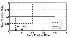
Figure 2: ROC curves for scoring functions f1subscript𝑓1f_{1} and f2subscript𝑓2f_{2} described in the above table on a sample containing 4 positive instances and 5 negative instances.

Partial AUC vs. Full AUC. It is important to note that for the AUC to take its maximum value of 1, a scoring function needs to rank the positive instances above all the negative instances. On the other hand, for the partial AUC in a specified interval [α,β]𝛼𝛽[\alpha,\beta] to take a value of 1, it is sufficient that a scoring function ranks the positives above a subset of the negative instances (specifically, above those in positions jα+1subscript𝑗𝛼1j_{\alpha}+1 to jβsubscript𝑗𝛽j_{\beta} in the ranking of negatives). Another key difference between the two evaluation measures is that the full AUC can be expressed as an expectation or sum of indicator terms over pairs of positive-negative instances (see Eq. (1)), whereas the partial AUC does not have such a simple additive structure. This is clearly evident in the definition in Eq. (2), where the set of negatives corresponding to FPR range [α,β]𝛼𝛽[\alpha,\beta] that appear in the inner summation is not fixed and can be different for different scoring functions f𝑓f.

We would also like to stress that a scoring function with a high AUC value need not be optimal in terms of partial AUC in a particular FPR range. This is illustrated in Figure 2, which shows scores assigned by two scoring functions f1subscript𝑓1f_{1} and f2subscript𝑓2f_{2} on a hypothetical sample of 4 positive and 6 negative instances, and the corresponding ROC curves. As can be seen, while f1subscript𝑓1f_{1} gives a higher AUC value, f2subscript𝑓2f_{2} has higher partial AUC in the FPR range [0.1,0.2]0.10.2[0.1,0.2]. This motivates the need to design algorithms that are tailored to directly optimize partial AUC.

2.2 Background on Structural SVM Framework for Full AUC

As a first step towards developing a method for optimizing the partial AUC, we shall provide some background on the popular structural SVM framework for maximizing the full AUC [18]. Unless otherwise specified, we shall assume that Xd𝑋superscript𝑑X\subseteq{\mathbb{R}}^{d} for some d+𝑑subscriptd\in{\mathbb{Z}}_{+} and shall consider linear scoring functions of the form f(x)=wx𝑓𝑥superscript𝑤top𝑥f(x)=w^{\top}x for some wd𝑤superscript𝑑w\in{\mathbb{R}}^{d}; the methods described will easily extend to non-linear functions / non-Euclidean instance spaces using kernels [46].

Hinge loss based surrogate. Given a training sample S𝑆S, our goal here is to find a scoring function that yields maximum empirical AUC on S𝑆S, or equivalently minimizes one minus the empirical AUC, given as follows:

R^AUC(w;S)=1mni=1mj=1n𝟏(wxi+wxj).subscript^𝑅AUC𝑤𝑆1𝑚𝑛superscriptsubscript𝑖1𝑚superscriptsubscript𝑗1𝑛1superscript𝑤topsuperscriptsubscript𝑥𝑖superscript𝑤topsuperscriptsubscript𝑥𝑗\widehat{R}_{\textup{{AUC}}}(w;\,S)\,=\,\frac{1}{mn}\sum_{i=1}^{m}\sum_{j=1}^{n}{\mathbf{1}}\big{(}w^{\top}x_{i}^{+}\leq w^{\top}x_{j}^{-}\big{)}. (3)

Owing to its discrete nature, minimizing this objective is a hard problem in general. One instead works with a convex proxy or surrogate objective for the above risk that is easier to optimize. A common approach is to replace the above indicator term with a pair-wise loss such as the pair-wise hinge loss, which for any scoring function f𝑓f and instances x+superscript𝑥x^{+} and xsuperscript𝑥x^{-} is defined as (1(wx+wx))+subscript1superscript𝑤topsuperscript𝑥superscript𝑤topsuperscript𝑥(1-(w^{\top}x^{+}-w^{\top}x^{-}))_{+}, where (z)+=max{0,z}subscript𝑧0𝑧(z)_{+}=\max\{0,z\}; this is clearly convex in w𝑤w and an upper bound on 𝟏(wx+wx)1superscript𝑤topsuperscript𝑥superscript𝑤topsuperscript𝑥{\mathbf{1}}\big{(}w^{\top}x^{+}\leq w^{\top}x^{-}\big{)}. The following is then the well-known pairwise hinge surrogate for the AUC risk:

R^AUChinge(w;S)=1mni=1mj=1n(1(wxi+wxj))+.subscriptsuperscript^𝑅hingeAUC𝑤𝑆1𝑚𝑛superscriptsubscript𝑖1𝑚superscriptsubscript𝑗1𝑛subscript1superscript𝑤topsuperscriptsubscript𝑥𝑖superscript𝑤topsuperscriptsubscript𝑥𝑗\widehat{R}^{\textup{{hinge}}}_{\textup{{AUC}}}(w;\,S)\,=\,\frac{1}{mn}\sum_{i=1}^{m}\sum_{j=1}^{n}(1-(w^{\top}x_{i}^{+}-w^{\top}x_{j}^{-}))_{+}. (4)

This surrogate is convex in w𝑤w, upper bounds the AUC risk, and is minimized by a scoring function that ranks positives instances above the negative instances with a sufficient margin of separation. It is also evident that one can minimize this objective over all model vectors w𝑤w using a standard convex optimization solver. In fact, there are several specialized methods available to solve (a regularized form of) this optimization problem [14, 17, 18]. For example, one popular approach is to solve the corresponding dual optimization problem using a coordinate descent type method [17].

On the other hand, the partial AUC has a more complex structure as the subset of negatives relevant to the given FPR range can be different for different scoring models; as a result, a surrogate obtained by replacing the indicators with the pairwise hinge loss turns out to be non-convex in general. The approach that we take for the partial AUC will instead make use of the structural SVM framework developed by Joachims (2005) for designing surrogate minimizing methods for general complex performance measures [18]. For the full AUC, it has been shown that this formulation recovers the corresponding hinge surrogate in Eq. (4) [19]. We give the details for AUC below, and in subsequent sections build on this formulation to construct and optimize convex surrogates for the partial AUC.

Structural SVM formulation. For any ordering of the training instances, we shall represent (errors in) the relative ordering of the m𝑚m positive instances in S+subscript𝑆S_{+} and n𝑛n negative instances in Ssubscript𝑆S_{-} via a matrix π=[πij]{0,1}m×n𝜋delimited-[]subscript𝜋𝑖𝑗superscript01𝑚𝑛\pi=[\pi_{ij}]\in\{0,1\}^{m\times n} as follows:

πij={1if xi+ is ranked below xj0if xi+ is ranked above xj.subscript𝜋𝑖𝑗cases1if xi+ is ranked below xj0if xi+ is ranked above xj.\pi_{ij}=\left\{\begin{array}[]{ll}1&~{}~{}\mbox{if $x^{+}_{i}$ is ranked \emph{below} $x^{-}_{j}$}\\[2.0pt] 0&~{}~{}\mbox{if $x^{+}_{i}$ is ranked above $x^{-}_{j}$.}\\ \end{array}\right.

Not all 2mnsuperscript2𝑚𝑛2^{mn} matrices in {0,1}m×nsuperscript01𝑚𝑛\{0,1\}^{m\times n} represent a valid relative ordering (due to transitivity requirements). We let Πm,nsubscriptΠ𝑚𝑛\Pi_{m,n} denote the set of all matrices in {0,1}m×nsuperscript01𝑚𝑛\{0,1\}^{m\times n} that do correspond to valid orderings. Clearly, the correct relative ordering πsuperscript𝜋\pi^{*} has πij=0i,jsubscriptsuperscript𝜋𝑖𝑗0for-all𝑖𝑗\pi^{*}_{ij}=0~{}\forall i,j. For any πΠm,n𝜋subscriptΠ𝑚𝑛\pi\in\Pi_{m,n}, we can define the AUC loss of π𝜋\pi with respect to πsuperscript𝜋\pi^{*} as

ΔAUC(π,π)=1mni=1mj=1nπi,j.subscriptΔAUCsuperscript𝜋𝜋1𝑚𝑛superscriptsubscript𝑖1𝑚superscriptsubscript𝑗1𝑛subscript𝜋𝑖𝑗\displaystyle\Delta_{\textup{{AUC}}}(\pi^{*},\pi)=\frac{1}{mn}\sum_{i=1}^{m}\sum_{j=1}^{n}\pi_{i,j}. (5)

It can be verified that for any π𝜋\pi that is consistent with scoring function wxsuperscript𝑤top𝑥w^{\top}x, ΔAUC(π,π)subscriptΔAUCsuperscript𝜋𝜋\Delta_{\textup{{AUC}}}(\pi^{*},\pi) evaluates to the AUC risk R^AUC(w;S)subscript^𝑅AUC𝑤𝑆\widehat{R}_{\textup{{AUC}}}(w;\,S) in Eq. (3).

Further, we shall also define a joint feature map between the input training sample and an output ordering matrix ϕ:(Xm×Xn)×Πm,nd:italic-ϕsuperscript𝑋𝑚superscript𝑋𝑛subscriptΠ𝑚𝑛superscript𝑑\phi:(X^{m}\times X^{n})\times\Pi_{m,n}{\,\rightarrow\,}{\mathbb{R}}^{d} as

ϕ(S,π)=1mni=1mj=1n(1πij)(xi+xj).italic-ϕ𝑆𝜋1𝑚𝑛superscriptsubscript𝑖1𝑚superscriptsubscript𝑗1𝑛1subscript𝜋𝑖𝑗subscriptsuperscript𝑥𝑖subscriptsuperscript𝑥𝑗\phi(S,\pi)=\frac{1}{mn}\sum_{i=1}^{m}\sum_{j=1}^{n}(1-\pi_{ij})(x^{+}_{i}-x^{-}_{j})\,.\vspace{-4pt} (6)

The above expression evaluates to a (normalized) sum of feature vector differences over all pairs of positive-negative instances in S𝑆S in which the positive instance is ordered by π𝜋\pi above the negative instance. This choice of ϕ(S,π)italic-ϕ𝑆𝜋\phi(S,\pi) ensures that for any fixed wd𝑤superscript𝑑w\in{\mathbb{R}}^{d}, maximizing wϕ(S,π)superscript𝑤topitalic-ϕ𝑆𝜋w^{\top}\phi(S,\pi) over πΠm,n𝜋subscriptΠ𝑚𝑛\pi\in\Pi_{m,n} yields an ordering matrix consistent with the scoring function wxsuperscript𝑤top𝑥w^{\top}x, and thus for which the loss term evaluates to R^AUC(w;S)subscript^𝑅AUC𝑤𝑆\widehat{R}_{\textup{{AUC}}}(w;\,S). The problem of optimizing the AUC now reduces to finding a wd𝑤superscript𝑑w\in{\mathbb{R}}^{d} for which the maximizer over πΠm,n𝜋subscriptΠ𝑚𝑛\pi\in\Pi_{m,n} of wϕ(S,π)superscript𝑤topitalic-ϕ𝑆𝜋w^{\top}\phi(S,\pi) has minimum AUC loss. This is approximated by the following structural SVM based relaxation of the AUC loss:

R^AUCstruct(w;S)=maxπΠm,n{ΔAUC(π,π)(wϕ(S,π)wϕ(S,π))}.subscriptsuperscript^𝑅structAUC𝑤𝑆𝜋subscriptΠ𝑚𝑛subscriptΔAUCsuperscript𝜋𝜋superscript𝑤topitalic-ϕ𝑆superscript𝜋superscript𝑤topitalic-ϕ𝑆𝜋\widehat{R}^{\textup{{struct}}}_{\textup{{AUC}}}(w;\,S)\,=\,\underset{\pi\,\in\,\Pi_{m,n}}{\max}\big{\{}\Delta_{\textup{{AUC}}}(\pi^{*},\pi)\,-\,(w^{\top}\phi(S,\pi^{*})-w^{\top}\phi(S,\pi))\big{\}}. (7)

Clearly, this surrogate is convex in w𝑤w as it is a maximum of linear functions in w𝑤w. Moreover, this is also an upper bound on the empirical AUC risk R^AUC(w;S)subscript^𝑅AUC𝑤𝑆\widehat{R}_{\textup{{AUC}}}(w;\,S): let π¯¯𝜋\bar{\pi} be the maximizer of wϕ(S,π)superscript𝑤topitalic-ϕ𝑆𝜋w^{\top}\phi(S,\pi) over Πm,nsubscriptΠ𝑚𝑛\Pi_{m,n}; then from the above definition R^AUCstruct(w;S)ΔAUC(π,π¯)(wϕ(S,π)wϕ(S,π¯))ΔAUC(π,π¯)=R^AUC(w;S)subscriptsuperscript^𝑅structAUC𝑤𝑆subscriptΔAUCsuperscript𝜋¯𝜋superscript𝑤topitalic-ϕ𝑆superscript𝜋superscript𝑤topitalic-ϕ𝑆¯𝜋subscriptΔAUCsuperscript𝜋¯𝜋subscript^𝑅AUC𝑤𝑆\widehat{R}^{\textup{{struct}}}_{\textup{{AUC}}}(w;\,S)\,\geq\,{\Delta_{\textup{{AUC}}}(\pi^{*},\bar{\pi})-(w^{\top}\phi(S,\pi^{*})-w^{\top}\phi(S,\bar{\pi}))}\,\geq\,\Delta_{\textup{{AUC}}}(\pi^{*},\bar{\pi})=\widehat{R}_{\textup{{AUC}}}(w;\,S).

Interestingly, this surrogate can be shown to be equivalent to the hinge-loss based surrogate in Eq. (4).

Theorem 1 (Joachims, 2006 [19]).

For any wd𝑤superscript𝑑w\in{\mathbb{R}}^{d} and training sample SXm×Xn𝑆superscript𝑋𝑚superscript𝑋𝑛S\in X^{m}\times X^{n}, R^AUCstruct(w;S)=R^AUChinge(w;S).subscriptsuperscript^𝑅structAUC𝑤𝑆subscriptsuperscript^𝑅hingeAUC𝑤𝑆\widehat{R}^{\textup{{struct}}}_{\textup{{AUC}}}(w;\,S)\,=\,\widehat{R}^{\textup{{hinge}}}_{\textup{{AUC}}}(w;\,S).

For completeness, we provide a proof for the theorem in Appendix A.1 (see Supplementary Material).

Thus the problem of minimizing a pairwise hinge surrogate for the AUC can be cast as one of optimizing the above structural SVM surrogate (along with a suitable regularizer), which results in the following SVM style convex (quadratic) program:

minw,ξ012w2+Cξsubscript𝑤𝜉012superscriptnorm𝑤2𝐶𝜉\min_{w,\,\xi\geq 0}\,\frac{1}{2}||w||^{2}+C\xi
s.t.πΠm,n:w(ϕ(S,π)ϕ(S,π))ΔAUC(π,π)ξ,:s.t.for-all𝜋subscriptΠ𝑚𝑛superscript𝑤topitalic-ϕ𝑆superscript𝜋italic-ϕ𝑆𝜋subscriptΔAUCsuperscript𝜋𝜋𝜉\text{s.t.}~{}~{}\forall\pi\in\Pi_{m,n}:~{}~{}w^{\top}\big{(}\phi(S,\pi^{*})-\phi(S,\pi)\big{)}~{}\geq~{}\Delta_{\textup{{AUC}}}(\pi^{*},\pi)-\xi\,,

where C>0𝐶0C>0 is a regularization parameter.

Cutting plane method. While the above optimization problem contains an exponential number of constraints (one for each πΠmn𝜋subscriptΠ𝑚𝑛\pi\in\Pi_{mn}), it can be solved efficiently using the cutting plane method [41]. Each iteration of this solver requires a combinatorial optimization over matrices in ΠmnsubscriptΠ𝑚𝑛\Pi_{mn}. By exploiting the simple structure of the AUC loss, this combinatorial problem can be decomposed into simpler ones, where each entry of the matrix can be optimized independently [18]. The cutting plane method is guaranteed to yield an ϵitalic-ϵ\epsilon-accurate solution in O(1/ϵ)𝑂1italic-ϵO(1/\epsilon) iterations [19]; in the case of the AUC, each iteration requires O((m+n)log(m+n))𝑂𝑚𝑛𝑚𝑛O((m+n)\log(m+n)) computational time. We elaborate on this solver in Section 4 when we develop a structural SVM approach for the partial AUC.

3 Candidate Surrogates for Partial AUC

As noted earlier, our goal in this paper is to design efficient methods for optimizing the partial AUC in a specified false positive range. In particular, given a training sample S=(S+,S)𝑆subscript𝑆subscript𝑆S=(S_{+},S_{-}), we wish to find a scoring function f(x)=wx𝑓𝑥superscript𝑤top𝑥f(x)=w^{\top}x that maximizes partial AUC in [α,β]𝛼𝛽[\alpha,\beta], or equivalently minimizes the following risk:

R^pAUC(α,β)(w;S)=1mjβi=1mj=jα+1jβ𝟏(wxi+wx(j)w).subscript^𝑅pAUC𝛼𝛽𝑤𝑆1𝑚subscript𝑗𝛽superscriptsubscript𝑖1𝑚superscriptsubscript𝑗subscript𝑗𝛼1subscript𝑗𝛽1superscript𝑤topsuperscriptsubscript𝑥𝑖superscript𝑤topsuperscriptsubscript𝑥subscript𝑗𝑤\displaystyle\widehat{R}_{\textup{{pAUC}}(\alpha,\beta)}(w;\,S)\,=\,\frac{1}{mj_{\beta}}\sum_{i=1}^{m}\sum_{j=j_{\alpha}+1}^{j_{\beta}}{\mathbf{1}}\big{(}w^{\top}x_{i}^{+}\leq w^{\top}x_{(j)_{w}}^{-}\big{)}. (8)

As before, optimizing this quantity directly is computationally hard in general. Hence, we work with a continuous surrogate objective that acts as a proxy for the above risk. As first-cut attempts at devising surrogates for the partial AUC, we replicate the two approaches used above for constructing surrogates for the full AUC, namely those based on the hinge loss and the structural SVM framework respectively. As we shall see, the surrogates obtained in both cases have certain drawbacks, requiring us to use a somewhat different approach.

3.1 Hinge Loss Based Surrogate

We begin by considering a hinge style surrogate for the partial AUC obtained by replacing the indicator functions in the partial AUC risk with the pairwise hinge loss.

R^pAUC(α,β)hinge(w;S)=1m(jβjα)i=1mj=jα+1jβ(1(wxi+wx(j)w))+.subscriptsuperscript^𝑅hingepAUC𝛼𝛽𝑤𝑆1𝑚subscript𝑗𝛽subscript𝑗𝛼superscriptsubscript𝑖1𝑚superscriptsubscript𝑗subscript𝑗𝛼1subscript𝑗𝛽subscript1superscript𝑤topsuperscriptsubscript𝑥𝑖superscript𝑤topsuperscriptsubscript𝑥subscript𝑗𝑤\widehat{R}^{\textup{{hinge}}}_{\textup{{pAUC}}(\alpha,\beta)}(w;\,S)\,=\,\frac{1}{m(j_{\beta}-j_{\alpha})}\sum_{i=1}^{m}\sum_{j=j_{\alpha}+1}^{j_{\beta}}\big{(}1\,-\,(w^{\top}x_{i}^{+}\,-\,w^{\top}x_{(j)_{w}}^{-})\big{)}_{+}. (9)

In the case of the full AUC (i.e. when the FPR interval is [0,1]01[0,1]), the hinge surrogate is convex in w𝑤w and can hence be optimized efficiently. However, the corresponding surrogate given above for the partial AUC turns out to be non-convex in general. This is because the surrogate is defined on only a subset of negative instances relevant to the given FPR range, and this subset can be different for different scoring functions.

Theorem 2.

Let 0<α<β0𝛼𝛽0<\alpha<\beta with jα>0subscript𝑗𝛼0j_{\alpha}>0. Then there exists a training sample SXm×Xn𝑆superscript𝑋𝑚superscript𝑋𝑛S\in X^{m}\times X^{n} for which the surrogate R^pAUC(α,β)hinge(w;S)subscriptsuperscript^𝑅hingepAUC𝛼𝛽𝑤𝑆\widehat{R}^{\textup{{hinge}}}_{\textup{{pAUC}}(\alpha,\beta)}(w;\,S) is non-convex in w𝑤w.

Proof (Sketch).

Consider the FPR range [n1n,1]𝑛1𝑛1\displaystyle\bigg{[}\frac{n-1}{n},1\bigg{]} where jα=n1>0subscript𝑗𝛼𝑛10j_{\alpha}=n-1>0 and jβ=nsubscript𝑗𝛽𝑛j_{\beta}=n. Here the hinge surrogate reduces to a ‘min’ of convex functions in w𝑤w and it is easy to see that there are samples S𝑆S where the surrogate is non-convex in w𝑤w. Note the same also holds for a general kthsuperscript𝑘thk^{\text{th}} order statistic of a set of convex functions in w𝑤w when k>1𝑘1k>1. In similar lines, one can construct a sample S𝑆S where the hinge surrogate is non-convex for more general FPR intervals. The details are provided in Appendix A.2 (see Supplementary Material). ∎

Fortunately, for the case where α=0𝛼0\alpha=0 and jα=nα=0subscript𝑗𝛼𝑛𝛼0j_{\alpha}=\lfloor n\alpha\rfloor=0, i.e. for FPR intervals of the form [0,β]0𝛽[0,\beta], the hinge loss based surrogate turns out to be convex. Here the surrogate is given by

R^pAUC(0,β)hinge(w;S)=1mjβi=1mj=1jβ(1(wxi+wx(j)w))+,subscriptsuperscript^𝑅hingepAUC0𝛽𝑤𝑆1𝑚subscript𝑗𝛽superscriptsubscript𝑖1𝑚superscriptsubscript𝑗1subscript𝑗𝛽subscript1superscript𝑤topsuperscriptsubscript𝑥𝑖superscript𝑤topsuperscriptsubscript𝑥subscript𝑗𝑤\widehat{R}^{\textup{{hinge}}}_{\textup{{pAUC}}(0,\beta)}(w;\,S)\,=\,\frac{1}{mj_{\beta}}\sum_{i=1}^{m}\sum_{j=1}^{j_{\beta}}\big{(}1\,-\,(w^{\top}x_{i}^{+}\,-\,w^{\top}x_{(j)_{w}}^{-})\big{)}_{+}, (10)

and we have:

Theorem 3.

Let β>0𝛽0\beta>0. For any training sample SXm×Xn𝑆superscript𝑋𝑚superscript𝑋𝑛S\in X^{m}\times X^{n}, the surrogate R^pAUC(0,β)hinge(w;S)subscriptsuperscript^𝑅hingepAUC0𝛽𝑤𝑆\widehat{R}^{\textup{{hinge}}}_{\textup{{pAUC}}(0,\beta)}(w;\,S) is convex in w𝑤w.

Proof.

Fix SXm×Xn𝑆superscript𝑋𝑚superscript𝑋𝑛S\in X^{m}\times X^{n}. Let w1,w2dsubscript𝑤1subscript𝑤2superscript𝑑w_{1},w_{2}\in{\mathbb{R}}^{d}. Let λ(0,1)𝜆01\lambda\in(0,1), and w~=λw1+(1λ)w2~𝑤𝜆subscript𝑤11𝜆subscript𝑤2\widetilde{w}=\lambda w_{1}+(1-\lambda)w_{2}. We wish to then show that

R^pAUC(0,β)hinge(w~;S)λR^pAUC(0,β)hinge(w1;S)+(1λ)R^pAUC(0,β)hinge(w2;S).subscriptsuperscript^𝑅hingepAUC0𝛽~𝑤𝑆𝜆subscriptsuperscript^𝑅hingepAUC0𝛽subscript𝑤1𝑆1𝜆subscriptsuperscript^𝑅hingepAUC0𝛽subscript𝑤2𝑆\widehat{R}^{\textup{{hinge}}}_{\textup{{pAUC}}(0,\beta)}(\widetilde{w};\,S)\,\leq\,\lambda\widehat{R}^{\textup{{hinge}}}_{\textup{{pAUC}}(0,\beta)}(w_{1};\,S)\,+\,(1-\lambda)\widehat{R}^{\textup{{hinge}}}_{\textup{{pAUC}}(0,\beta)}(w_{2};\,S).

Define for any negative xsuperscript𝑥x^{-}, r(w;S+,x)=1mi=1m𝟏(wxi+wx)𝑟𝑤subscript𝑆superscript𝑥1𝑚superscriptsubscript𝑖1𝑚1superscript𝑤topsuperscriptsubscript𝑥𝑖superscript𝑤topsuperscript𝑥r(w;\,S_{+},x^{-})=\frac{1}{m}\sum_{i=1}^{m}{\mathbf{1}}\big{(}w^{\top}x_{i}^{+}\leq w^{\top}x^{-}\big{)}. Notice that r(w;S+,x)𝑟𝑤subscript𝑆superscript𝑥r(w;\,S_{+},x^{-}) is convex in w𝑤w, and moreover is monotonically increasing in the score wxsuperscript𝑤topsuperscript𝑥w^{\top}x^{-} assigned to xsuperscript𝑥x^{-}. Expanding the left hand side from the desired inequality,

R^pAUC(0,β)hinge(w~;S)subscriptsuperscript^𝑅hingepAUC0𝛽~𝑤𝑆\displaystyle{\widehat{R}^{\textup{{hinge}}}_{\textup{{pAUC}}(0,\beta)}(\widetilde{w};\,S)} =\displaystyle= 1jβj=1jβr(w~;S+,x(j)w~)1subscript𝑗𝛽superscriptsubscript𝑗1subscript𝑗𝛽𝑟~𝑤superscript𝑆superscriptsubscript𝑥subscript𝑗~𝑤\displaystyle\frac{1}{j_{\beta}}\sum_{j=1}^{j_{\beta}}r(\widetilde{w};S^{+},x_{(j)_{\widetilde{w}}}^{-})
\displaystyle\leq λ1jβj=1jβr(w1;S+,x(j)w~)+(1λ)1jβj=1jβr(w2;S+,x(j)w~)𝜆1subscript𝑗𝛽superscriptsubscript𝑗1subscript𝑗𝛽𝑟subscript𝑤1superscript𝑆superscriptsubscript𝑥subscript𝑗~𝑤1𝜆1subscript𝑗𝛽superscriptsubscript𝑗1subscript𝑗𝛽𝑟subscript𝑤2superscript𝑆superscriptsubscript𝑥subscript𝑗~𝑤\displaystyle\lambda\frac{1}{j_{\beta}}\sum_{j=1}^{j_{\beta}}r(w_{1};S^{+},x_{(j)_{\widetilde{w}}}^{-})\,\,+\,\,(1-\lambda)\frac{1}{j_{\beta}}\sum_{j=1}^{j_{\beta}}r(w_{2};S^{+},x_{(j)_{\widetilde{w}}}^{-})
\displaystyle\leq λ1jβj=1jβr(w1;S+,x(j)w1)+(1λ)1jβj=1jβr(w2;S+,x(j)w2)𝜆1subscript𝑗𝛽superscriptsubscript𝑗1subscript𝑗𝛽𝑟subscript𝑤1superscript𝑆superscriptsubscript𝑥subscript𝑗subscript𝑤11𝜆1subscript𝑗𝛽superscriptsubscript𝑗1subscript𝑗𝛽𝑟subscript𝑤2superscript𝑆superscriptsubscript𝑥subscript𝑗subscript𝑤2\displaystyle\lambda\frac{1}{j_{\beta}}\sum_{j=1}^{j_{\beta}}r(w_{1};S^{+},x_{(j)_{w_{1}}}^{-})\,\,+\,\,(1-\lambda)\frac{1}{j_{\beta}}\sum_{j=1}^{j_{\beta}}r(w_{2};S^{+},x_{(j)_{w_{2}}}^{-})
=\displaystyle= λR^pAUC(0,β)hinge(w1;S)+(1λ)R^pAUC(0,β)hinge(w2;S).𝜆subscriptsuperscript^𝑅hingepAUC0𝛽subscript𝑤1𝑆1𝜆subscriptsuperscript^𝑅hingepAUC0𝛽subscript𝑤2𝑆\displaystyle\lambda\widehat{R}^{\textup{{hinge}}}_{\textup{{pAUC}}(0,\beta)}(w_{1};\,S)\,+\,(1-\lambda)\widehat{R}^{\textup{{hinge}}}_{\textup{{pAUC}}(0,\beta)}(w_{2};\,S).

The second step follows by convexity of r𝑟r (notice that the negative instances here are still ranked by w~~𝑤\widetilde{w}). The third step uses the fact that r(w1;S+,x)𝑟subscript𝑤1superscript𝑆superscript𝑥r(w_{1};S^{+},x^{-}) is monotonic in w1xsuperscriptsubscript𝑤1topsuperscript𝑥w_{1}^{\top}x^{-} and r(w2;S+,x)𝑟subscript𝑤2superscript𝑆superscript𝑥r(w_{2};S^{+},x^{-}) is monotonic in w2xsuperscriptsubscript𝑤2topsuperscript𝑥w_{2}^{\top}x^{-}; hence the top ranked negative jβsubscript𝑗𝛽j_{\beta} instances according to w1subscript𝑤1w_{1} will yield higher summation value than those ranked according to w~~𝑤\widetilde{w}, and similarly for w2subscript𝑤2w_{2}. This completes the proof. ∎

Despite the hinge surrogate for FPR intervals of the form [0,β]0𝛽[0,\beta] being convex, it is not immediate how the resulting optimization problem can be solved efficiently. For instance, a common approach for optimizing the full AUC surrogate is to derive and solve the corresponding dual optimization problem. Since the surrogate for the partial AUC is defined on a subset of negative instances that can be different for different scoring functions, even deriving the dual problem for the hinge partial AUC surrogate turns out to be non-trivial.

3.2 Naïve Structural SVM Surrogate

As an alternative to the hinge surrogate, we next consider constructing a convex surrogate for the partial AUC by a direct application of the structural SVM formulation described in the previous section for the AUC. Specifically, we consider the surrogate obtained by replacing the loss term in the structural SVM surrogate for the AUC in Eq. (7) with an appropriate loss for the partial AUC in [α,β]𝛼𝛽[\alpha,\beta]:

ΔpAUC(π,π)=1m(jβjα)i=1mj=jα+1jβπi,(j)π,subscriptΔpAUCsuperscript𝜋𝜋1𝑚subscript𝑗𝛽subscript𝑗𝛼superscriptsubscript𝑖1𝑚superscriptsubscript𝑗subscript𝑗𝛼1subscript𝑗𝛽subscript𝜋𝑖subscript𝑗𝜋\displaystyle\Delta_{\textup{{pAUC}}}(\pi^{*},\pi)=\frac{1}{m(j_{\beta}-j_{\alpha})}\sum_{i=1}^{m}\sum_{j=j_{\alpha}+1}^{j_{\beta}}\pi_{i,(j)_{\pi}},

where (j)πsubscript𝑗𝜋(j)_{\pi} denotes the index of the j𝑗j-th ranked negative instance by any fixed ordering of instances consistent with π𝜋\pi; the resulting surrogate is given by:

R^pAUC(α,β)struct(w;S)=maxπΠm,n{ΔpAUC(π,π)(wϕ(S,π)wϕ(S,π))}.subscriptsuperscript^𝑅structpAUC𝛼𝛽𝑤𝑆𝜋subscriptΠ𝑚𝑛subscriptΔpAUCsuperscript𝜋𝜋superscript𝑤topitalic-ϕ𝑆superscript𝜋superscript𝑤topitalic-ϕ𝑆𝜋\widehat{R}^{\text{struct}}_{\textup{{pAUC}}(\alpha,\beta)}(w;S)\,=\,\underset{\pi\,\in\,\Pi_{m,n}}{\max}\big{\{}\Delta_{\textup{{pAUC}}}(\pi^{*},\pi)\,-\,(w^{\top}\phi(S,\pi^{*})-w^{\top}\phi(S,\pi))\big{\}}. (11)

As with the AUC, this surrogate serves as a convex upper bound for the partial AUC risk in Eq. (8). At first glance, this surrogate does appear as a good proxy for the partial AUC risk. However, on closer look, one can show that this surrogate does have drawbacks, as explained below.

Recall that with the AUC, the structural SVM surrogate is equivalent to the corresponding hinge surrogate (see Theorem 1). However, even for the special case of partial AUC in FPR intervals of the form [0,β]0𝛽[0,\beta] (where the hinge surrogate is convex), the above structural SVM surrogate turns out to be looser convex upper bound on the partial AUC risk than the hinge surrogate in Eq. (9). In particular, one can show that in its simplified form, the above structural SVM surrogate for the partial AUC contains redundant terms that penalize misrankings of the scoring function with respect to negative instances outside the relevant FPR range, and in particular, in positions jβ+1,,nsubscript𝑗𝛽1𝑛j_{\beta}+1,\ldots,n of the ranked list. These additional terms appear because the joint feature map ϕitalic-ϕ\phi in the surrogate is defined on all negative instances and not just the ones relevant to the given FPR range (see Eq. (6)). Clearly, these terms disrupt the emphasis of the surrogate on the specified FPR interval. The details can be found in the earlier conference versions of this paper [29, 30] and are left out here to keep the exposition simple.

Thus a naïve application of the structural SVM formulation yields a loose surrogate for the partial AUC. Of course, one could look at tightening the surrogate by restricting the joint feature map to only a subset of negative instances; however, it is not immediate how this can be done, as the subset of negatives relevant to the given FPR interval can be different for different scoring models w𝑤w, while the definition of the joint feature map in the structural SVM framework needs to be independent of w𝑤w.

The approach that we take constructs a tighter surrogate for the partial AUC by making use of the structural SVM framework in a manner that suitably exploits the structure of the partial AUC performance measure. In particular, we first rewrite the partial AUC risk as a maximum of a certain term over subsets of negatives, and compute a convex approximation to the inner term using the structural SVM setup; in the rewritten formulation, the joint feature maps need to be defined on only a subset of the negative instances. The resulting surrogate is convex and is equivalent to the corresponding hinge surrogate for [0,β]0𝛽[0,\beta] intervals in Eq. (10). For general FPR intervals [α,β]𝛼𝛽[\alpha,\beta], the proposed surrogate can be seen as a tighter convex relaxation to the partial AUC risk compared to the naïve structural SVM surrogate.

(a) R^AUC(w;S)R^AUChinge(w;S)=R^AUCstruct(w;S)subscript^𝑅AUC𝑤𝑆subscriptsuperscript^𝑅hingeAUC𝑤𝑆subscriptsuperscript^𝑅structAUC𝑤𝑆\widehat{R}_{\textup{{AUC}}}(w;S)\,\leq\,\widehat{R}^{\textup{{hinge}}}_{\textup{{AUC}}}(w;S)\,=\,\widehat{R}^{\textup{{struct}}}_{\textup{{AUC}}}(w;S)
(b) R^pAUC(0,β)(w;S)R^pAUC(0,β)hinge(w;S)=R^pAUC(0,β)tight(w;S)R^pAUC(0,β)struct(w;S)subscript^𝑅pAUC0𝛽𝑤𝑆subscriptsuperscript^𝑅hingepAUC0𝛽𝑤𝑆subscriptsuperscript^𝑅tightpAUC0𝛽𝑤𝑆subscriptsuperscript^𝑅structpAUC0𝛽𝑤𝑆\widehat{R}_{\textup{{pAUC}}(0,\beta)}(w;S)\,\leq\,\widehat{R}^{\textup{{hinge}}}_{\textup{{pAUC}}(0,\beta)}(w;S)\,=\,{\color[rgb]{0,0,1}\widehat{R}^{\textup{{tight}}}_{\textup{{pAUC}}(0,\beta)}(w;S)}\,\leq\,\widehat{R}^{\text{struct}}_{\textup{{pAUC}}(0,\beta)}(w;S)
(c) R^pAUC(α,β)(w;S)R^pAUC(α,β)hinge(w;S)R^pAUC(α,β)tight(w;S)R^pAUC(α,β)struct(w;S)subscript^𝑅pAUC𝛼𝛽𝑤𝑆subscriptsuperscript^𝑅hingepAUC𝛼𝛽𝑤𝑆subscriptsuperscript^𝑅tightpAUC𝛼𝛽𝑤𝑆subscriptsuperscript^𝑅structpAUC𝛼𝛽𝑤𝑆\widehat{R}_{\textup{{pAUC}}(\alpha,\beta)}(w;S)\,\leq\,{\color[rgb]{1,0,0}\widehat{R}^{\textup{{hinge}}}_{\textup{{pAUC}}(\alpha,\beta)}(w;S)}\,\leq\,{\color[rgb]{0,0,1}\widehat{R}^{\textup{{tight}}}_{\textup{{pAUC}}(\alpha,\beta)}(w;S)}\,\leq\,\widehat{R}^{\text{struct}}_{\textup{{pAUC}}(\alpha,\beta)}(w;S)
Figure 3: Relationship between surrogates for (a) AUC and for partial AUC in (b) [0,β]0𝛽[0,\beta] and (c) [α,β]𝛼𝛽[\alpha,\beta]. Here wd𝑤superscript𝑑w\in{\mathbb{R}}^{d} is a fixed model vector and S𝑆S is the given training sample. Those colored in blue are the tight convex structural SVM surrogates that we optimize using the cutting plane method (see Sections 4 and 5); the one in red is the non-convex hinge surrogate that we optimize using a DC programming method (see Section 6).

A summary of the surrogates discussed here is given in Figure 3. Among the surrogates considered, the hinge surrogates serve as the tightest upper bound on the partial AUC risk, but are not necessarily convex; on the other hand, the naïve structural SVM surrogates are convex, but yield a looser upper bound. The structural SVM based surrogates proposed in this paper (highlighted in blue) are convex and also serve as tighter upper bounds compared to the naïve surrogates; moreover in the case of [0,β]0𝛽[0,\beta] intervals, the proposed surrogate is equivalent to the corresponding hinge surrogate.

We also provide a cutting plane method to optimize the prescribed surrogates. Unlike the full AUC, here the combinatorial optimization required in each iteration of the solver does not decompose easily into simpler problems. One of our main contributions is a polynomial time algorithm for solving this combinatorial optimization for the partial AUC. The details are provided for the [0,β]0𝛽[0,\beta] case in Section 4 and for the [α,β]𝛼𝛽[\alpha,\beta] case in Section 5. In addition to methods that optimize convex structural SVM surrogates on the partial AUC, we also develop a method for directly optimizing the non-convex hinge surrogate for general FPR intervals using difference-of-convex programming; this approach is explained in Section 6.

4 Structural SVM Approach for Partial AUC in [0,β]0𝛽[0,\beta]

We start by developing a method for optimizing the partial AUC in FPR intervals [0,β]0𝛽[0,\beta]:

R^pAUC(0,β)(w;S)=1mjβi=1mj=1jβ𝟏(wxi+wx(j)w).subscript^𝑅pAUC0𝛽𝑤𝑆1𝑚subscript𝑗𝛽superscriptsubscript𝑖1𝑚superscriptsubscript𝑗1subscript𝑗𝛽1superscript𝑤topsuperscriptsubscript𝑥𝑖superscript𝑤topsuperscriptsubscript𝑥subscript𝑗𝑤\displaystyle\widehat{R}_{\textup{{pAUC}}(0,\beta)}(w;\,S)\,=\,\frac{1}{mj_{\beta}}\sum_{i=1}^{m}\sum_{j=1}^{j_{\beta}}{\mathbf{1}}\big{(}w^{\top}x_{i}^{+}\leq w^{\top}x_{(j)_{w}}^{-}\big{)}. (12)

We saw in the previous section that the hinge loss based surrogate is convex in this case, but it was not immediate how this objective can be optimized efficiently. We also saw that a naïve application of the structural SVM framework results in a surrogate that is a looser convex approximation to the partial AUC risk than the hinge surrogate.

Our approach makes use of the structural SVM formulation in a manner that allows us to construct a tighter convex surrogate for the partial AUC, which in this case is equivalent to the corresponding hinge surrogate. The key idea here is that the partial AUC risk in [0,β]0𝛽[0,\beta] can be written as maximum over subsets of negatives of the full AUC risk evaluated on all positives and the given subset of negatives. The structural SVM formulation described earlier in Section 2 for the full AUC can then be leveraged to design a convex surrogate, and to optimize it efficiently using a cutting plane solver.

4.1 Tight Structural SVM Surrogate for pAUC in [0,β]0𝛽[0,\beta]

For any subset of negatives ZS𝑍subscript𝑆Z\subseteq S_{-}, let R^AUC(w;S+,Z)subscript^𝑅AUC𝑤subscript𝑆𝑍\widehat{R}_{\textup{{AUC}}}(w;\,S_{+},\,Z) denote the full AUC risk of scoring function wxsuperscript𝑤top𝑥w^{\top}x evaluated on a sample containing all the positives S+subscript𝑆S_{+} and the subset of negatives Z𝑍Z. Then the partial AUC risk of wxsuperscript𝑤top𝑥w^{\top}x is simply the value of this quantity on the top ranked jβsubscript𝑗𝛽j_{\beta} negatives; this can be shown to be equivalent to the maximum value of R^AUC(w;S+,Z)subscript^𝑅AUC𝑤subscript𝑆𝑍\widehat{R}_{\textup{{AUC}}}(w;\,S_{+},\,Z) over all subsets of negatives Z𝑍Z of size jβsubscript𝑗𝛽j_{\beta}.

Theorem 4.

For any wd𝑤superscript𝑑w\in{\mathbb{R}}^{d} and training sample S=(S+,S)Xm×Xn𝑆subscript𝑆subscript𝑆superscript𝑋𝑚superscript𝑋𝑛S=(S_{+},S_{-})\in X^{m}\times X^{n},

R^pAUC(0,β)(w;S)subscript^𝑅pAUC0𝛽𝑤𝑆\displaystyle\vspace{-10pt}\widehat{R}_{\textup{{pAUC}}(0,\beta)}(w;\,S) =\displaystyle= maxZS,|Z|=jβ1mjβi=1mxZ𝟏(wxi+wx)subscriptformulae-sequence𝑍subscript𝑆𝑍subscript𝑗𝛽1𝑚subscript𝑗𝛽superscriptsubscript𝑖1𝑚subscriptsuperscript𝑥𝑍1superscript𝑤topsuperscriptsubscript𝑥𝑖superscript𝑤topsuperscript𝑥\displaystyle\max_{Z\subseteq S_{-},\,|Z|=j_{\beta}}\,\frac{1}{mj_{\beta}}\sum_{i=1}^{m}\sum_{x^{-}\in Z}{\mathbf{1}}(w^{\top}x_{i}^{+}\leq w^{\top}x^{-}) (13)
=\displaystyle= maxZS,|Z|=jβR^AUC(w;S+,Z).subscriptformulae-sequence𝑍subscript𝑆𝑍subscript𝑗𝛽subscript^𝑅AUC𝑤subscript𝑆𝑍\displaystyle\max_{Z\subseteq S_{-},\,|Z|=j_{\beta}}\,\widehat{R}_{\textup{{AUC}}}(w;\,S_{+},\,Z).
Proof.

Define for any negative xsuperscript𝑥x^{-}, r(w;S+,x)=1mi=1m𝟏(wxi+wx)𝑟𝑤subscript𝑆superscript𝑥1𝑚superscriptsubscript𝑖1𝑚1superscript𝑤topsuperscriptsubscript𝑥𝑖superscript𝑤topsuperscript𝑥\displaystyle r(w;\,S_{+},x^{-})=\frac{1}{m}\sum_{i=1}^{m}{\mathbf{1}}\big{(}w^{\top}x_{i}^{+}\leq w^{\top}x^{-}\big{)}. Notice that r(w;S+,x)𝑟𝑤subscript𝑆superscript𝑥r(w;\,S_{+},x^{-}) is monotonically increasing in the score wxsuperscript𝑤topsuperscript𝑥w^{\top}x^{-} assigned to xsuperscript𝑥x^{-}. Thus R^AUC(w;S+,Z)=1jβxZr(w;S+,x)subscript^𝑅AUC𝑤subscript𝑆𝑍1subscript𝑗𝛽subscriptsuperscript𝑥𝑍𝑟𝑤subscript𝑆superscript𝑥\widehat{R}_{\textup{{AUC}}}(w;\,S_{+},\,Z)=\frac{1}{j_{\beta}}\sum_{x^{-}\in Z}\,r(w;\,S_{+},x^{-}) takes the highest value when Z𝑍Z contains the top ranked jβsubscript𝑗𝛽j_{\beta} negatives, and by definition (see Eq. (12)), this maximum value is equal to the partial AUC risk of the given scoring function in the FPR range [0,β]0𝛽[0,\beta]. ∎

Having expressed the partial AUC risk in [0,β]0𝛽[0,\beta] in terms of the full AUC risk on a subset of instances, we can devise a convex surrogate for the evaluation measure by constructing a convex approximation to the full AUC term using the structural SVM formulation explained earlier in Section 2.2.

In particular, let us define truncated ordering matrices π{0,1}m×jβ𝜋superscript01𝑚subscript𝑗𝛽\pi\in\{0,1\}^{m\times j_{\beta}} for positive instances S+subscript𝑆S_{+} and any subset Z={z1,,zjβ}S𝑍subscript𝑧1subscript𝑧subscript𝑗𝛽subscript𝑆Z=\{z_{1},\ldots,z_{j_{\beta}}\}\subseteq S_{-} of negative instances as

πij={1if xi+ is ranked below zj0if xi+ is ranked above zj.subscript𝜋𝑖𝑗cases1if xi+ is ranked below zj0if xi+ is ranked above zj.\pi_{ij}=\left\{\begin{array}[]{ll}1&~{}~{}\mbox{if $x^{+}_{i}$ is ranked {below} $z_{j}$}\\[2.0pt] 0&~{}~{}\mbox{if $x^{+}_{i}$ is ranked above $z_{j}$.}\\ \end{array}\right.

The set of all valid orderings is denoted as Πm,jβsubscriptΠ𝑚subscript𝑗𝛽\Pi_{m,j_{\beta}}, and the correct ordering is given by π=𝟎m×jβsuperscript𝜋superscript0𝑚subscript𝑗𝛽\pi^{*}=\mathbf{0}^{m\times j_{\beta}}. Also redefine the joint feature map for m𝑚m positive and jβsubscript𝑗𝛽j_{\beta} negatives: ϕ:Xm×Xjβd:italic-ϕsuperscript𝑋𝑚superscript𝑋subscript𝑗𝛽superscript𝑑\phi:X^{m}\times X^{j_{\beta}}{\,\rightarrow\,}{\mathbb{R}}^{d}. As seen earlier, the following is then a convex upper bound on the inner AUC term in Eq. (13):

maxπΠm,jβ{ΔAUC(π,π)w(ϕ((S+,Z),π)ϕ((S+,Z),π)}.\underset{\pi\,\in\,\Pi_{m,j_{\beta}}}{\max}\big{\{}\Delta_{\textup{{AUC}}}(\pi^{*},\pi)\,-\,w^{\top}\big{(}\phi((S_{+},Z),\pi^{*})-\phi((S_{+},Z),\pi\big{)}\big{\}}.

Replacing the AUC term in Eq. (13) with the above expression gives us a surrogate that upper bounds the partial AUC risk in [0,β]0𝛽[0,\beta]:

R^pAUC(0,β)tight(w;S)subscriptsuperscript^𝑅tightpAUC0𝛽𝑤𝑆\displaystyle\widehat{R}^{\textup{{tight}}}_{\textup{{pAUC}}(0,\beta)}(w;\,S) =maxZS,|Z|=jβmaxπΠm,jβ{ΔAUC(π,π)w(ϕ((S+,Z),π)ϕ((S+,Z),π)},\displaystyle=\displaystyle\max_{Z\subseteq S_{-},\,|Z|=j_{\beta}}\,\underset{\pi\,\in\,\Pi_{m,j_{\beta}}}{\max}\big{\{}\Delta_{\textup{{AUC}}}(\pi^{*},\pi)\,-\,w^{\top}\big{(}\phi((S_{+},Z),\pi^{*})-\phi((S_{+},Z),\pi\big{)}\big{\}}, (14)

where the πijsubscript𝜋𝑖𝑗\pi_{ij}’s index over all positive instances, and over negative instances in the corresponding subset Z𝑍Z in the outer argmax.

Clearly, the prescribed surrogate objective is convex in w𝑤w as it is a maximum of convex functions in w𝑤w. In fact, this surrogate is equivalent to the corresponding hinge surrogate for partial AUC in [0,β]0𝛽[0,\beta] in Eq. (10). More specifically, we know from Theorem 1 that the structural SVM expression used above to approximate the inner full AUC term is same as the hinge surrogate for the AUC:

R^pAUC(0,β)tight(w;S)subscriptsuperscript^𝑅tightpAUC0𝛽𝑤𝑆\displaystyle{\widehat{R}^{\textup{{tight}}}_{\textup{{pAUC}}(0,\beta)}(w;\,S)} =\displaystyle= maxZS,|Z|=jβ1mjβi=1mxZ(1(wxi+wx))+.subscriptformulae-sequence𝑍subscript𝑆𝑍subscript𝑗𝛽1𝑚subscript𝑗𝛽superscriptsubscript𝑖1𝑚subscriptsuperscript𝑥𝑍subscript1superscript𝑤topsuperscriptsubscript𝑥𝑖superscript𝑤topsuperscript𝑥\displaystyle\max_{Z\subseteq S_{-},\,|Z|=j_{\beta}}\,\frac{1}{mj_{\beta}}\sum_{i=1}^{m}\sum_{x^{-}\in Z}\big{(}1-(w^{\top}x_{i}^{+}-w^{\top}x^{-})\big{)}_{+}. (15)

At first glance, this appears different from the hinge surrogate for [0,β]0𝛽[0,\beta] range in Eq. (10). However, as seen next, the above maximum in attained at the top jβsubscript𝑗𝛽j_{\beta} negatives according to w𝑤w, which clearly implies that the two surrogates are equivalent.

Proposition 1.

Let Z¯={z¯1,,z¯jβ}¯𝑍subscript¯𝑧1subscript¯𝑧subscript𝑗𝛽\bar{Z}=\{\bar{z}_{1},\ldots,\bar{z}_{j_{\beta}}\} be the set of negative instances ranked in the top jβsubscript𝑗𝛽j_{\beta} positions (among all negative instances in Ssubscript𝑆S_{-}, in descending order of scores) by wxsuperscript𝑤top𝑥w^{\top}x. Then the maximum value of the objective in Eq. (15) (or equivalently in Eq. (14)) is attained at Z¯¯𝑍\bar{Z}.

Proof.

Define for any xsuperscript𝑥x^{-}, r(w;S+,x)=1mi=1m(1(wxi+wx))+𝑟𝑤subscript𝑆superscript𝑥1𝑚superscriptsubscript𝑖1𝑚subscript1superscript𝑤topsuperscriptsubscript𝑥𝑖superscript𝑤topsuperscript𝑥\displaystyle r(w;\,S_{+},x^{-})=\frac{1}{m}\sum_{i=1}^{m}\big{(}1-(w^{\top}x_{i}^{+}-w^{\top}x^{-})\big{)}_{+}. The proof then follows the same argument used in proving Theorem 4 and uses the fact that r𝑟r is monotonically increasing in the scores on negative instances. ∎

The following result then follows directly from the above proposition.

Theorem 5.

For any wd𝑤superscript𝑑w\in{\mathbb{R}}^{d} and training sample SXm×Xn𝑆superscript𝑋𝑚superscript𝑋𝑛S\in X^{m}\times X^{n}, R^pAUC(0,β)tight(w;S)=R^pAUC(0,β)hinge(w;S).subscriptsuperscript^𝑅tightpAUC0𝛽𝑤𝑆subscriptsuperscript^𝑅hingepAUC0𝛽𝑤𝑆\widehat{R}^{\textup{{tight}}}_{\textup{{pAUC}}(0,\beta)}(w;\,S)\,=\,\widehat{R}^{\textup{{hinge}}}_{\textup{{pAUC}}(0,\beta)}(w;\,S).

Also notice that unlike the naïve structural SVM surrogate in Eq. (11), the joint feature map ϕitalic-ϕ\phi in the proposed surrogate in Eq. (14) is not defined on all negatives, but only on a subset of negatives; consequently, this surrogate does not contain additional redundant terms, and is thus tighter than the naïve surrogate [30] (see Figure 3). We shall next develop a cutting plane method for optimizing this surrogate.

Algorithm 1 Cutting Plane Method for SVMpAUCsubscriptSVMpAUC\text{SVM}_{\textup{{pAUC}}} in [α,β]𝛼𝛽[\alpha,\beta]
1:  Inputs: S=(S+,S),α,β,C,ϵ𝑆subscript𝑆subscript𝑆𝛼𝛽𝐶italic-ϵS=(S_{+},S_{-}),~{}\alpha,~{}\beta,~{}C,~{}\epsilon
2:  Initialize:
3:  If α=0𝛼0\alpha=0:
4:        Hw(Z,π)ΔAUC(π,π)w(ϕ((S+,Z),π)ϕ((S+,Z),π))subscript𝐻𝑤𝑍𝜋subscriptΔAUCsuperscript𝜋𝜋superscript𝑤topitalic-ϕsubscript𝑆𝑍superscript𝜋italic-ϕsubscript𝑆𝑍𝜋H_{w}(Z,\pi)\,\equiv\,\Delta_{\textup{{AUC}}}(\pi^{*},\pi)-w^{\top}\big{(}\phi((S_{+},Z),\pi^{*})-\phi((S_{+},Z),\pi)\big{)}
5:  else:
6:        Hw(Z,π)ΔpAUCtr(π,π)w(ϕ((S+,Z),π)ϕ((S+,Z),π))subscript𝐻𝑤𝑍𝜋subscriptsuperscriptΔtrpAUCsuperscript𝜋𝜋superscript𝑤topitalic-ϕsubscript𝑆𝑍superscript𝜋italic-ϕsubscript𝑆𝑍𝜋H_{w}(Z,\pi)\,\equiv\,\Delta^{\text{tr}}_{\textup{{pAUC}}}(\pi^{*},\pi)-w^{\top}\big{(}\phi((S_{+},Z),\pi^{*})-\phi((S_{+},Z),\pi)\big{)}   (see Eq. (17))
7:  𝒞=𝒞\mathcal{C}=\emptyset
8:  Repeat
9:        (w,ξ)=argminw,ξ012w2+Cξ𝑤𝜉𝑤𝜉0argmin12superscriptnorm𝑤2𝐶𝜉(w,\xi)=\underset{w,\,\xi\geq 0}{\operatorname{argmin}}\,\frac{1}{2}||w||^{2}+C\xi s.t.(Z,π)𝒞:ξHw(Z,π):s.t.for-all𝑍𝜋𝒞𝜉subscript𝐻𝑤𝑍𝜋\hskip 7.11317pt~{}~{}\text{s.t.}~{}~{}\hskip 7.11317pt\forall(Z,\pi)\in{\mathcal{C}}:~{}~{}\xi\geq H_{w}(Z,\pi)
10:        (Z¯,π¯)=argmaxZS,|Z|=jβπΠm,jβHw(Z,π)¯𝑍¯𝜋formulae-sequence𝑍subscript𝑆𝑍subscript𝑗𝛽𝜋subscriptΠ𝑚subscript𝑗𝛽argmaxsubscript𝐻𝑤𝑍𝜋(\bar{Z},\bar{\pi})=\underset{\begin{subarray}{c}Z\subseteq S_{-},\,|Z|=j_{\beta}\\ \pi\,\in\,\Pi_{m,j_{\beta}}\end{subarray}}{\operatorname{argmax}}~{}H_{w}(Z,\pi)      (compute the most violated constraint)
11:        𝒞=𝒞{(Z¯,π¯)}𝒞𝒞¯𝑍¯𝜋{\mathcal{C}}={\mathcal{C}}\cup\{(\bar{Z},\bar{\pi})\}
12:  Until  Hw(Z¯,π¯)ξ+ϵsubscript𝐻𝑤¯𝑍¯𝜋𝜉italic-ϵH_{w}(\bar{Z},\bar{\pi})\,\leq\,\xi+\epsilon
13:  Output: w𝑤w

4.2 Cutting Plane Method for Optimizing R^pAUC(0,β)tightsubscriptsuperscript^𝑅tightpAUC0𝛽\widehat{R}^{\textup{{tight}}}_{\textup{{pAUC}}(0,\beta)}

We would like to minimize the proposed surrogate in Eq. (14) with an additional regularization term on w𝑤w. This yields the (convex) quadratic program given below.

minw,ξ012w2+Cξsubscript𝑤𝜉012superscriptnorm𝑤2𝐶𝜉\min_{w,\,\xi\geq 0}\,\frac{1}{2}||w||^{2}+C\xi
s.t.ZS,|Z|=jβ,πΠm,jβ::formulae-sequences.t.for-all𝑍subscript𝑆formulae-sequence𝑍subscript𝑗𝛽for-all𝜋subscriptΠ𝑚subscript𝑗𝛽absent\displaystyle\text{s.t.}~{}~{}\forall Z\subseteq S_{-},\,|Z|=j_{\beta},~{}~{}\forall\pi\in\Pi_{m,j_{\beta}}:~{}~{}
w(ϕ((S+,Z),π)ϕ((S+,Z),π))ΔAUC(π,π)ξ.superscript𝑤topitalic-ϕsubscript𝑆𝑍superscript𝜋italic-ϕsubscript𝑆𝑍𝜋subscriptΔAUCsuperscript𝜋𝜋𝜉\displaystyle w^{\top}\big{(}\phi((S_{+},Z),\pi^{*})-\phi((S_{+},Z),\pi)\big{)}~{}\geq~{}\Delta_{\textup{{AUC}}}(\pi^{*},\pi)-\xi\,.

Notice that the optimization problem has an exponential number of constraints, one for each subset of negative instances of size jβsubscript𝑗𝛽j_{\beta} and matrix πΠm,jβ𝜋subscriptΠ𝑚subscript𝑗𝛽\pi\in\Pi_{m,j_{\beta}}. As with the full AUC, we use the cutting plane method to solve this problem. The idea behind this method is that for any ϵ>0italic-ϵ0\epsilon>0, a small subset of the constraints is sufficient to find an ϵitalic-ϵ\epsilon-approximate solution to the problem [19]. In particular, the method starts with an empty constraint set 𝒞=𝒞{\mathcal{C}}=\emptyset, and on each iteration, adds the most violated constraint to 𝒞𝒞{\mathcal{C}}, and solves a tighter relaxation of the optimization problem in the subsequent iteration; this continues until no constraint is violated by more than ϵitalic-ϵ\epsilon (see Algorithm 1).

It is known that for any fixed regularization parameter C>0𝐶0C>0 and tolerance ϵ>0italic-ϵ0\epsilon>0, the cutting plane method converges in O(C/ϵ+log(1/C))𝑂𝐶italic-ϵ1𝐶O(C/\epsilon+\log(1/C)) iterations, and will yield a surrogate value within ϵitalic-ϵ\epsilon of the minimum value [19]. Since in each iteration, the quadratic program needed to be solved grows only by a single constraint, the primary bottleneck in the algorithm is the combinatorial optimization (over subsets of negatives and ordering matrices) required to find the most violated constraint (line 10).

Finding most-violated constraint. The specific combinatorial optimization problem that we wish to solve can be stated as:

argmaxZS,|Z|=jβπΠm,jβ{ΔAUC(π,π)w(ϕ((S+,Z),π)ϕ((S+,Z),π)}.\underset{\begin{subarray}{c}Z\subseteq S_{-},\,|Z|=j_{\beta}\\ \pi\,\in\,\Pi_{m,j_{\beta}}\end{subarray}}{\operatorname{argmax}}\big{\{}\Delta_{\textup{{AUC}}}(\pi^{*},\pi)\,-\,w^{\top}\big{(}\phi((S_{+},Z),\pi^{*})-\phi((S_{+},Z),\pi\big{)}\big{\}}.

In the case of AUC, where jβ=nsubscript𝑗𝛽𝑛j_{\beta}=n, the above argmax is only over ordering matrices in Πm,nsubscriptΠ𝑚𝑛\Pi_{m,n}, and can be easily computed by exploiting the additive form of the AUC loss and in particular, by neatly decomposing the problem into one where each πijsubscript𝜋𝑖𝑗\pi_{ij} can be chosen independently [18]. In the case of the partial AUC in [0,β]0𝛽[0,\beta], the decomposition is not as straightforward as the argmax is also over subsets of negatives.

Algorithm 2 Find Most-Violated Constraint for pAUC in [0,β]0𝛽[0,\beta]
1:  Inputs: S=(S+,S)𝑆subscript𝑆subscript𝑆S=(S_{+},S_{-}), β𝛽\beta, w𝑤w
2:  Set Z¯={z¯1,,z¯jβ}¯𝑍subscript¯𝑧1subscript¯𝑧subscript𝑗𝛽\bar{Z}=\{\bar{z}_{1},\ldots,\bar{z}_{j_{\beta}}\} as the set of instances ranked in the top jβsubscript𝑗𝛽j_{\beta} positions among Ssubscript𝑆S_{-} (in descending order of scores) by wxsuperscript𝑤top𝑥w^{\top}x
3:  π¯ij=𝟏(wxi+wz¯j1)i{1,,m},j{1,,jβ}formulae-sequencesubscript¯𝜋𝑖𝑗1superscript𝑤topsubscriptsuperscript𝑥𝑖superscript𝑤topsubscript¯𝑧𝑗1for-all𝑖1𝑚𝑗1subscript𝑗𝛽\bar{\pi}_{ij}={\mathbf{1}}(w^{\top}x^{+}_{i}\,-\,w^{\top}\bar{z}_{j}\leq 1)~{}~{}~{}\forall i\in\{1,\ldots,m\},~{}j\in\{1,\ldots,j_{\beta}\}
4:  Output: Z¯,π¯¯𝑍¯𝜋\bar{Z},\bar{\pi}

Reduction to simpler problems. We however know from Proposition 1 that the above argmax is attained at the top jβsubscript𝑗𝛽j_{\beta} negatives Z¯={z¯1,,z¯jβ}¯𝑍subscript¯𝑧1subscript¯𝑧subscript𝑗𝛽\bar{Z}=\{\bar{z}_{1},\ldots,\bar{z}_{j_{\beta}}\} according to w𝑤w, and all that remains is to compute the optimal ordering matrix in Πm,jβsubscriptΠ𝑚subscript𝑗𝛽\Pi_{m,j_{\beta}} keeping Z¯¯𝑍\bar{Z} fixed; the optimization problem can then be decomposed easily. In particular, having fixed the subset Z¯¯𝑍\bar{Z}, the combinatorial optimization problem becomes equivalent to:

argmaxπΠm,jβ1mjβi=1mj=1jβπij(1w(xi+z¯j)).𝜋subscriptΠ𝑚subscript𝑗𝛽argmax1𝑚subscript𝑗𝛽superscriptsubscript𝑖1𝑚superscriptsubscript𝑗1subscript𝑗𝛽subscript𝜋𝑖𝑗1superscript𝑤topsubscriptsuperscript𝑥𝑖subscript¯𝑧𝑗\underset{\pi\,\in\,\Pi_{m,j_{\beta}}}{\operatorname{argmax}}\,\frac{1}{mj_{\beta}}\sum_{i=1}^{m}\sum_{j=1}^{j_{\beta}}\pi_{ij}\big{(}1\,-\,w^{\top}(x^{+}_{i}-\bar{z}_{j})\big{)}. (OP1)

Now consider solving a relaxed form of OP1 over all matrices in {0,1}m×jβsuperscript01𝑚subscript𝑗𝛽\{0,1\}^{m\times j_{\beta}}. The objective now decomposes into a sum of terms involving individual elements πi,j{0,1}subscript𝜋𝑖𝑗01\pi_{i,j}\in\{0,1\} and can be maximized by optimizing each term separately; the optimal matrix is then given by π¯ij=𝟏(wxi+wz¯j 1)subscript¯𝜋𝑖𝑗1superscript𝑤topsubscriptsuperscript𝑥𝑖superscript𝑤topsubscript¯𝑧𝑗1\bar{\pi}_{ij}={\mathbf{1}}(w^{\top}x^{+}_{i}\,-\,w^{\top}\bar{z}_{j}\,\leq\,1). It can be seen that this optimal matrix π¯¯𝜋\bar{\pi} is in fact a valid ordering matrix in Πm,jβsubscriptΠ𝑚subscript𝑗𝛽\Pi_{m,j_{\beta}}, as it corresponds to ordering of instances where the positives are scored according to wxsuperscript𝑤top𝑥w^{\top}x and the negatives are scored according to wx+1superscript𝑤top𝑥1w^{\top}x+1. Hence π¯¯𝜋\bar{\pi} is also a solution to the original unrelaxed form of OP1 for fixed Z¯¯𝑍\bar{Z}, and thus (Z¯,π¯)¯𝑍¯𝜋(\bar{Z},\bar{\pi}) gives us the desired most-violated constraint.

Time complexity. A straightforward implementation to compute the above solution (see Algorithm 2) would take computational time O(mjβ+nlog(n))𝑂𝑚subscript𝑗𝛽𝑛𝑛O(mj_{\beta}+n\log(n)) (assuming score evaluations on instances can be done in unit time). Using a more compact representation of the orderings [18], however, this can be further reduced to O((m+jβ)log(m+jβ)+nlog(n))𝑂𝑚subscript𝑗𝛽𝑚subscript𝑗𝛽𝑛𝑛O((m+j_{\beta})\log(m+j_{\beta})+n\log(n)). The details can be found in Appendix B.1. Thus computing the most-violated constraint for the partial AUC in a small interval [0,β]0𝛽[0,\beta] is faster than that for the full AUC [18]; this is because the number of negative instances relevant to the given FPR range over which the most-violated constraint is computed is smaller for the partial AUC. On the other hand, it turns out that in practice, the number of iterations required by the cutting plane method to converge (and in turn the number of calls to the given combinatorial optimization) is often higher for partial AUC compared to AUC; we will elaborate this when we discuss our experimental results in Section 8.

We have presented an efficient method for optimizing the structural SVM surrogate for the partial AUC in the [0,β]0𝛽[0,\beta] range, which we saw was equivalent to the hinge surrogate. We next proceed to algorithms for optimizing partial AUC in a general FPR interval [α,β]𝛼𝛽[\alpha,\beta].

5 Structural SVM Approach for Partial AUC in [α,β]𝛼𝛽[\alpha,\beta]

Recall that the partial AUC in a general FPR interval [α,β]𝛼𝛽[\alpha,\beta] is given by:

R^pAUC(α,β)(w;S)=1m(jβjα)i=1mj=jα+1jβ𝟏(wxi+wx(j)w).subscript^𝑅pAUC𝛼𝛽𝑤𝑆1𝑚subscript𝑗𝛽subscript𝑗𝛼superscriptsubscript𝑖1𝑚superscriptsubscript𝑗subscript𝑗𝛼1subscript𝑗𝛽1superscript𝑤topsuperscriptsubscript𝑥𝑖superscript𝑤topsuperscriptsubscript𝑥subscript𝑗𝑤\displaystyle\widehat{R}_{\textup{{pAUC}}(\alpha,\beta)}(w;\,S)\,=\,\frac{1}{m(j_{\beta}-j_{\alpha})}\sum_{i=1}^{m}\sum_{j=j_{\alpha}+1}^{j_{\beta}}{\mathbf{1}}\big{(}w^{\top}x_{i}^{+}\leq w^{\top}x_{(j)_{w}}^{-}\big{)}. (16)

We have already seen in Section 3 that in this case, the simple hinge surrogate (obtained by replacing the indicator terms in the above risk by the pairwise hinge loss) is not necessarily convex. We have also seen that a naïve application of the structural SVM formulation to the above risk yields a surrogate with redundant additional terms involving negative instances outside the specified FPR range. As with the [0,β]0𝛽[0,\beta] case, we now apply the structural SVM framework in a manner that yields a tighter convex surrogate for the partial AUC risk; of course, in this case, the resulting convex surrogate is not equivalent to the non-convex hinge surrogate, but as we explain later, can be seen as a convex relaxation to the hinge surrogate.

Again, the main idea here is to rewrite the partial AUC risk as a maximum of a certain term over subsets of negatives, and use the structural SVM formulation to compute a convex approximation to the inner term. We provide an efficient cutting plane method for solving the resulting optimization problem; here the combinatorial optimization step for finding the most-violated constraint in the cutting plane solver does not admit a decomposition involving individual matrix entries. We show that by using a suitable reformulation of the problem over a restricted search space, the optimization can be still reduced into simpler ones, but now involving individual rows of the ordering matrix. In Section 6, we shall also look at an approach for directly optimizing the non-convex hinge surrogate for general FPR ranges.

5.1 Tight Structural SVM Surrogate for pAUC in [α,β]𝛼𝛽[\alpha,\beta]

We begin by describing the construction of the tight structural SVM surrogate. Just as the partial AUC risk in [0,β]0𝛽[0,\beta] could be written as a maximum over subsets of negative instances of the full AUC risk evaluated on this subset (see Theorem 4), the partial AUC risk in [α,β]𝛼𝛽[\alpha,\beta] can also be written as a maximum of a certain term over subsets of negative instances of size jβsubscript𝑗𝛽j_{\beta}.

Theorem 6.

For any wd𝑤superscript𝑑w\in{\mathbb{R}}^{d} and training sample S=(S+,S)Xm×Xn𝑆subscript𝑆subscript𝑆superscript𝑋𝑚superscript𝑋𝑛S=(S_{+},S_{-})\in X^{m}\times X^{n},

R^pAUC(α,β)(w;S)subscript^𝑅pAUC𝛼𝛽𝑤𝑆\displaystyle\widehat{R}_{\textup{{pAUC}}(\alpha,\beta)}(w;\,S) =\displaystyle= maxZS,|Z|=jβR~(w;S+,Z),subscriptformulae-sequence𝑍subscript𝑆𝑍subscript𝑗𝛽~𝑅𝑤subscript𝑆𝑍\displaystyle\max_{Z\subseteq S_{-},\,|Z|=j_{\beta}}\,\widetilde{R}(w;\,S_{+},\,Z),

where for any subset of negative instances Z={z1,,zjβ}𝑍subscript𝑧1subscript𝑧subscript𝑗𝛽Z=\{z_{1},\ldots,z_{j_{\beta}}\} that (w.l.o.g.) satisfy wz1wzjβsuperscript𝑤topsubscript𝑧1superscript𝑤topsubscript𝑧subscript𝑗𝛽w^{\top}z_{1}\geq\ldots\geq w^{\top}z_{j_{\beta}},

R~(w;S+,Z)=1m(jβjα)i=1mj=jα+1jβ𝟏(wxi+wzj).~𝑅𝑤subscript𝑆𝑍1𝑚subscript𝑗𝛽subscript𝑗𝛼superscriptsubscript𝑖1𝑚superscriptsubscript𝑗subscript𝑗𝛼1subscript𝑗𝛽1superscript𝑤topsuperscriptsubscript𝑥𝑖superscript𝑤topsubscript𝑧𝑗\widetilde{R}(w;\,S_{+},\,Z)=\frac{1}{m(j_{\beta}-j_{\alpha})}\sum_{i=1}^{m}\sum_{j=j_{\alpha}+1}^{j_{\beta}}{\mathbf{1}}\big{(}w^{\top}x_{i}^{+}\leq w^{\top}z_{j}\big{)}.
Proof.

As in Theorem 4, define for any xsuperscript𝑥x^{-}, r(w;S+,x)=1mi=1m𝟏(wxi+wx)𝑟𝑤subscript𝑆superscript𝑥1𝑚superscriptsubscript𝑖1𝑚1superscript𝑤topsuperscriptsubscript𝑥𝑖superscript𝑤topsuperscript𝑥\displaystyle r(w;\,S_{+},x^{-})=\frac{1}{m}\sum_{i=1}^{m}{\mathbf{1}}\big{(}w^{\top}x_{i}^{+}\leq w^{\top}x^{-}\big{)}. Thus R~(w;S+,Z)~𝑅𝑤subscript𝑆𝑍\widetilde{R}(w;\,S_{+},\,Z) evaluates to the (scaled) average value of this quantity on the bottom ranked jβjαsubscript𝑗𝛽subscript𝑗𝛼j_{\beta}-j_{\alpha} negatives within Z𝑍Z by w𝑤w. Moreover, r(w;S+,x)𝑟𝑤subscript𝑆superscript𝑥r(w;\,S_{+},x^{-}) is monotonically increasing in the score wxsuperscript𝑤topsuperscript𝑥w^{\top}x^{-} assigned to xsuperscript𝑥x^{-}. As a result, R~(w;S+,Z)~𝑅𝑤subscript𝑆𝑍\widetilde{R}(w;\,S_{+},\,Z) takes the highest value when Z𝑍Z contains negatives in the top jβsubscript𝑗𝛽j_{\beta} positions in the ranking of all negatives in Ssubscript𝑆S_{-} by w𝑤w. By the definition in Eq. (16), this maximum value is equal to the partial AUC risk of the scoring function in [α,β]𝛼𝛽[\alpha,\beta]. ∎

Note when α=0𝛼0\alpha=0, the term R~(w;S+,Z)~𝑅𝑤subscript𝑆𝑍\widetilde{R}(w;\,S_{+},\,Z) is the full AUC risk on the sample (S+,Z)subscript𝑆𝑍(S_{+},Z), recovering our previous result in Theorem 4. In this case, we directly made use of the structural SVM formulation for the full AUC to construct a convex approximation for this term. However, when α>0𝛼0\alpha>0, R~(w;S+,Z)~𝑅𝑤subscript𝑆𝑍\widetilde{R}(w;\,S_{+},\,Z) is more complex and can be essentially seen as (a scaled version of) partial AUC risk in the FPR range [jα/jβ,1]subscript𝑗𝛼subscript𝑗𝛽1\big{[}{j_{\alpha}}/{j_{\beta}},1\big{]} defined on a subset of instances (S+,Z)subscript𝑆𝑍(S_{+},Z); we will hence have to rework the structural SVM formulation for R~~𝑅\widetilde{R}, as described next.

Convex upper bound on R~~𝑅\widetilde{R}. In particular, we describe how the structural SVM framework can be used to construct a convex upper bound on the inner term R~~𝑅\widetilde{R}, and thus obtain a convex surrogate for the partial AUC risk in [α,β]𝛼𝛽[\alpha,\beta]. Restricting ourselves to truncated ordering matrices πΠm,jβ𝜋subscriptΠ𝑚subscript𝑗𝛽\pi\in\Pi_{m,j_{\beta}} defined for m𝑚m positives and a subset of jβsubscript𝑗𝛽j_{\beta} negatives, let us again use (j)πsubscript𝑗𝜋(j)_{\pi} to denote the index of the j𝑗j-th ranked negative instance by any fixed ordering of instances consistent with π𝜋\pi (note that all such orderings yield the same value of R~~𝑅\widetilde{R}). We further define the loss term for the truncated ordering matrices:

ΔpAUCtr(π,π)=1m(jβjα)i=1mj=jα+1jβπi,(j)π.subscriptsuperscriptΔtrpAUCsuperscript𝜋𝜋1𝑚subscript𝑗𝛽subscript𝑗𝛼superscriptsubscript𝑖1𝑚superscriptsubscript𝑗subscript𝑗𝛼1subscript𝑗𝛽subscript𝜋𝑖subscript𝑗𝜋\displaystyle\Delta^{\text{tr}}_{\textup{{pAUC}}}(\pi^{*},\pi)=\frac{1}{m(j_{\beta}-j_{\alpha})}\sum_{i=1}^{m}\sum_{j=j_{\alpha}+1}^{j_{\beta}}\pi_{i,(j)_{\pi}}. (17)

Given that this loss is defined on a subset of instances, as noted above, it can be seen as the partial AUC loss in a scaled interval [jα/jβ,1]subscript𝑗𝛼subscript𝑗𝛽1\big{[}{j_{\alpha}}/{j_{\beta}},1\big{]}. The following is then a convex upper bound on R~~𝑅\widetilde{R}:

maxπΠm,jβ{ΔpAUCtr(π,π)w(ϕ((S+,Z),π)ϕ((S+,Z),π)},\displaystyle\underset{\pi\,\in\,\Pi_{m,j_{\beta}}}{\max}\big{\{}\Delta^{\text{tr}}_{\textup{{pAUC}}}(\pi^{*},\pi)\,-\,w^{\top}\big{(}\phi((S_{+},Z),\pi^{*})-\phi((S_{+},Z),\pi\big{)}\big{\}},

and replacing R~~𝑅\widetilde{R} in the rewritten partial AUC risk in Theorem 6 with the above expression gives us the following upper bounding surrogate:

R^pAUC(α,β)tight(w;S)=maxZS,|Z|=jβmaxπΠm,jβ{ΔpAUCtr(π,π)w(ϕ((S+,Z),π)ϕ((S+,Z),π)}.\displaystyle\widehat{R}^{\textup{{tight}}}_{\textup{{pAUC}}(\alpha,\beta)}(w;\,S)\,\,=\,\,\max_{Z\subseteq S_{-},\,|Z|=j_{\beta}}\,\underset{\pi\,\in\,\Pi_{m,j_{\beta}}}{\max}\big{\{}\Delta^{\text{tr}}_{\textup{{pAUC}}}(\pi^{*},\pi)\,-\,w^{\top}\big{(}\phi((S_{+},Z),\pi^{*})-\phi((S_{+},Z),\pi\big{)}\big{\}}. (18)

The surrogate is a maximum of convex functions in w𝑤w, and is hence convex in w𝑤w. Even here, it turns out the above maximum is attained by the top jβsubscript𝑗𝛽j_{\beta} negatives according to w𝑤w.

Proposition 2.

Let Z¯={z¯1,,z¯jβ}¯𝑍subscript¯𝑧1subscript¯𝑧subscript𝑗𝛽\bar{Z}=\{\bar{z}_{1},\ldots,\bar{z}_{j_{\beta}}\} be the set of instances in the top jβsubscript𝑗𝛽j_{\beta} positions in the ranking of negative instances (in descending order of scores) by wxsuperscript𝑤top𝑥w^{\top}x. Then the maximum value of the objective in Eq. (18) is attained at Z¯¯𝑍\bar{Z}.

Proof.

For any subset of negative instances Z={z1,,zjβ}S𝑍subscript𝑧1subscript𝑧subscript𝑗𝛽subscript𝑆Z=\{{z}_{1},\ldots,{z}_{j_{\beta}}\}\subseteq S_{-}, we assume w.l.o.g. that wz1wzjβsuperscript𝑤topsubscript𝑧1superscript𝑤topsubscript𝑧subscript𝑗𝛽w^{\top}z_{1}\geq\ldots\geq w^{\top}z_{j_{\beta}} (this ensures that the identity of each zjsubscript𝑧𝑗z_{j} is unique). Expanding the objective in Eq. (18) then gives us:

maxZ={z1,,zjβ}SmaxπΠm,jβ1m(jβjα)i=1m[j=jα+1jβπi(j)πj=1jβπijwxi++j=1jβπijwzj].subscript𝑍subscript𝑧1subscript𝑧subscript𝑗𝛽subscript𝑆subscript𝜋subscriptΠ𝑚subscript𝑗𝛽1𝑚subscript𝑗𝛽subscript𝑗𝛼superscriptsubscript𝑖1𝑚delimited-[]superscriptsubscript𝑗subscript𝑗𝛼1subscript𝑗𝛽subscript𝜋𝑖subscript𝑗𝜋superscriptsubscript𝑗1subscript𝑗𝛽subscript𝜋𝑖𝑗superscript𝑤topsuperscriptsubscript𝑥𝑖superscriptsubscript𝑗1subscript𝑗𝛽subscript𝜋𝑖𝑗superscript𝑤topsubscript𝑧𝑗\displaystyle{\max_{Z=\{{z}_{1},\ldots,{z}_{j_{\beta}}\}\subseteq S_{-}}\,\max_{\pi\,\in\,\Pi_{m,j_{\beta}}}\frac{1}{m(j_{\beta}-j_{\alpha})}\sum_{i=1}^{m}\bigg{[}\sum_{j=j_{\alpha}+1}^{j_{\beta}}\pi_{i(j)_{\pi}}\,-\,\sum_{j=1}^{j_{\beta}}\pi_{ij}\,w^{\top}x_{i}^{+}\,+\,\sum_{j=1}^{j_{\beta}}\pi_{ij}\,w^{\top}z_{j}\bigg{]}}.

Interchanging the two max over finite sets, we equivalently have:

1m(jβjα)maxπΠm,jβ[i=1m[j=jα+1jβπi(j)πj=1jβπijwxi+]+maxZ={z1,,zjβ}Sj=1jβqjwzj],1𝑚subscript𝑗𝛽subscript𝑗𝛼subscript𝜋subscriptΠ𝑚subscript𝑗𝛽superscriptsubscript𝑖1𝑚delimited-[]superscriptsubscript𝑗subscript𝑗𝛼1subscript𝑗𝛽subscript𝜋𝑖subscript𝑗𝜋superscriptsubscript𝑗1subscript𝑗𝛽subscript𝜋𝑖𝑗superscript𝑤topsuperscriptsubscript𝑥𝑖subscript𝑍subscript𝑧1subscript𝑧subscript𝑗𝛽subscript𝑆superscriptsubscript𝑗1subscript𝑗𝛽subscript𝑞𝑗superscript𝑤topsubscript𝑧𝑗\displaystyle\frac{1}{m(j_{\beta}-j_{\alpha})}\max_{\pi\,\in\,\Pi_{m,j_{\beta}}}\bigg{[}\sum_{i=1}^{m}\bigg{[}\sum_{j=j_{\alpha}+1}^{j_{\beta}}\pi_{i(j)_{\pi}}-\sum_{j=1}^{j_{\beta}}\pi_{ij}\,w^{\top}x_{i}^{+}\bigg{]}\,+\,\max_{Z=\{{z}_{1},\ldots,{z}_{j_{\beta}}\}\subseteq S_{-}}\sum_{j=1}^{j_{\beta}}q_{j}\,w^{\top}z_{j}\bigg{]},

where qj=i=1mπijsubscript𝑞𝑗superscriptsubscript𝑖1𝑚subscript𝜋𝑖𝑗q_{j}=\sum_{i=1}^{m}\pi_{ij} is a positive integer between 0 and m𝑚m. Clearly, the only term in the above objective that depends on instances in Z𝑍Z is the third term. For any fixed π𝜋\pi (or equivalent q𝑞q), this term is maximized when the subset Z𝑍Z contains the negatives with the highest scores by w𝑤w and in particular, the top jβsubscript𝑗𝛽j_{\beta} ranked negatives by w𝑤w.∎

Unlike the partial AUC in [0,β]0𝛽[0,\beta], the above structural SVM surrogate is not equivalent to the non-convex hinge surrogate in Eq. (9) for [α,β]𝛼𝛽[\alpha,\beta] intervals and is a looser upper bound on the partial AUC risk. On the other hand, compared to the naïve structural SVM surrogate in Eq. (11) for the [α,β]𝛼𝛽[\alpha,\beta] range, the joint feature map here is only defined on a subset of negatives, and as a result, the proposed surrogate is tighter and lays more emphasis on good performance in the given range [30] (see Figure 3). This will become clear from the characterization provided below.

5.2 Characterization for R^pAUC(α,β)tightsubscriptsuperscript^𝑅tightpAUC𝛼𝛽\widehat{R}^{\textup{{tight}}}_{\textup{{pAUC}}(\alpha,\beta)}

Before proceeding to develop a method for optimizing the proposed structural SVM surrogate for [α,β]𝛼𝛽[\alpha,\beta] intervals, we analyze how the surrogate is related to the original partial AUC risk in Eq. (16), and to the other surrogates discussed in Section 3. These relationships were obvious for the [0,β]0𝛽[0,\beta] case, as the prescribed structural SVM surrogate there was exactly equivalent to the associated hinge surrogate; for the [α,β]𝛼𝛽[\alpha,\beta], it is not immediate from the surrogate whether it closely mimics the partial AUC risk. We know so far that the proposed structural SVM surrogate for [α,β]𝛼𝛽[\alpha,\beta] intervals upper bounds the partial AUC risk; below we give a more detailed characterization:555We note that in the characterization result provided in the conference version of this paper [30] (Theorem 2), there are no terms η[0,α]subscript𝜂0𝛼\eta_{[0,\alpha]} and η[0,α]+subscriptsuperscript𝜂0𝛼\eta^{+}_{[0,\alpha]}; we have corrected this error here.

Theorem 7.

Let 0<α<β10𝛼𝛽10<\alpha<\beta\leq 1. Then for any sample SXm×Xn𝑆superscript𝑋𝑚superscript𝑋𝑛S\in X^{m}\times X^{n} and wd𝑤superscript𝑑w\in{\mathbb{R}}^{d}:

R^pAUC(α,β)hinge,+(w;S)+η[0,α]+(w)R^pAUC(α,β)tight(w;S)R^pAUC(α,β)hinge(w;S)+η[0,α](w),subscriptsuperscript^𝑅hingepAUC𝛼𝛽𝑤𝑆subscriptsuperscript𝜂0𝛼𝑤subscriptsuperscript^𝑅tightpAUC𝛼𝛽𝑤𝑆subscriptsuperscript^𝑅hingepAUC𝛼𝛽𝑤𝑆subscript𝜂0𝛼𝑤\displaystyle\widehat{R}^{\textup{{hinge}},+}_{\textup{{pAUC}}(\alpha,\beta)}(w;S)\,+\,\eta^{+}_{[0,\alpha]}(w)~{}~{}\leq~{}~{}\widehat{R}^{\textup{{tight}}}_{\textup{{pAUC}}(\alpha,\beta)}(w;S)~{}~{}\leq~{}~{}\widehat{R}^{\textup{{hinge}}}_{\textup{{pAUC}}(\alpha,\beta)}(w;S)\,+\,\eta_{[0,\alpha]}(w),

where R^pAUC(α,β)hingesubscriptsuperscript^𝑅hingepAUC𝛼𝛽\widehat{R}^{\textup{{hinge}}}_{\textup{{pAUC}}(\alpha,\beta)} is the hinge surrogate in Eq. (9) and R^pAUC(α,β)hinge,+subscriptsuperscript^𝑅hingepAUC𝛼𝛽\widehat{R}^{\textup{{hinge}},+}_{\textup{{pAUC}}(\alpha,\beta)} is a version of this surrogate defined on a subset of positive instances:

R^pAUC(α,β)hinge,+(w;S)=1m(jβjα)i:wxi+<wx(jα)wj=1jα(1w(xi+x(j)w))+,subscriptsuperscript^𝑅hingepAUC𝛼𝛽𝑤𝑆1𝑚subscript𝑗𝛽subscript𝑗𝛼subscript:𝑖superscript𝑤topsubscriptsuperscript𝑥𝑖superscript𝑤topsubscriptsuperscript𝑥subscriptsubscript𝑗𝛼𝑤superscriptsubscript𝑗1subscript𝑗𝛼subscript1superscript𝑤topsuperscriptsubscript𝑥𝑖subscriptsuperscript𝑥subscript𝑗𝑤\displaystyle\widehat{R}^{\textup{{hinge}},+}_{\textup{{pAUC}}(\alpha,\beta)}(w;S)=\frac{1}{m(j_{\beta}-j_{\alpha})}\sum_{i:w^{\top}x^{+}_{i}<w^{\top}x^{-}_{(j_{\alpha})_{w}}}\sum_{j=1}^{j_{\alpha}}\big{(}1-w^{\top}(x_{i}^{+}-x^{-}_{(j)_{w}})\big{)}_{+},

while η[0,α]subscript𝜂0𝛼\eta_{[0,\alpha]} and η[0,α]+subscriptsuperscript𝜂0𝛼\eta^{+}_{[0,\alpha]} are positive terms which penalize misrankings against negatives in the FPR range [0,α]0𝛼[0,\alpha] with a margin of zero:

η[0,α](w)=1m(jβjα)i=1mj=1jα(w(xi+x(j)w))+;subscript𝜂0𝛼𝑤1𝑚subscript𝑗𝛽subscript𝑗𝛼superscriptsubscript𝑖1𝑚superscriptsubscript𝑗1subscript𝑗𝛼subscriptsuperscript𝑤topsuperscriptsubscript𝑥𝑖subscriptsuperscript𝑥subscript𝑗𝑤\eta_{[0,\alpha]}(w)=\frac{1}{m(j_{\beta}-j_{\alpha})}\sum_{i=1}^{m}\sum_{j=1}^{j_{\alpha}}\big{(}-w^{\top}(x_{i}^{+}-x^{-}_{(j)_{w}})\big{)}_{+};
η[0,α]+(w)=1m(jβjα)i:wxi+<wx(jα)wj=1jα(w(xi+x(j)w))+.subscriptsuperscript𝜂0𝛼𝑤1𝑚subscript𝑗𝛽subscript𝑗𝛼subscript:𝑖superscript𝑤topsubscriptsuperscript𝑥𝑖superscript𝑤topsubscriptsuperscript𝑥subscriptsubscript𝑗𝛼𝑤superscriptsubscript𝑗1subscript𝑗𝛼subscriptsuperscript𝑤topsuperscriptsubscript𝑥𝑖subscriptsuperscript𝑥subscript𝑗𝑤\eta^{+}_{[0,\alpha]}(w)=\frac{1}{m(j_{\beta}-j_{\alpha})}\sum_{i:w^{\top}x^{+}_{i}<w^{\top}x^{-}_{(j_{\alpha})_{w}}}\sum_{j=1}^{j_{\alpha}}\big{(}-w^{\top}(x_{i}^{+}-x^{-}_{(j)_{w}})\big{)}_{+}.

Moreover, if |wxi+wxj|1i{1,,m},j{1,,n}formulae-sequencesuperscript𝑤topsubscriptsuperscript𝑥𝑖superscript𝑤topsubscriptsuperscript𝑥𝑗1for-all𝑖1𝑚𝑗1𝑛|w^{\top}x^{+}_{i}-w^{\top}x^{-}_{j}|\geq 1\,\,\forall\,i\in\{1,\ldots,m\},\,j\in\{1,\ldots,n\}, then the lower and upper bounds match and we have:

R^pAUC(α,β)tight(w;S)=R^pAUC(α,β)hinge(w;S)+η[0,α](w).subscriptsuperscript^𝑅tightpAUC𝛼𝛽𝑤𝑆subscriptsuperscript^𝑅hingepAUC𝛼𝛽𝑤𝑆subscript𝜂0𝛼𝑤\widehat{R}^{\textup{{tight}}}_{\textup{{pAUC}}(\alpha,\beta)}(w;S)=\widehat{R}^{\textup{{hinge}}}_{\textup{{pAUC}}(\alpha,\beta)}(w;S)\,+\,\eta_{[0,\alpha]}(w).

The proof is provided in Appendix A.3. Note that in both the lower and upper bounds, certain positive-negative pairs are penalized with a larger margin than others; in particular, those involving the negative instances in positions jα+1subscript𝑗𝛼1j_{\alpha}+1 to jβsubscript𝑗𝛽j_{\beta} are penalized with a margin of 1, while the rest are penalized with zero margin. This confirms the surrogate’s focus on a select portion of the ROC curve in the range [α,β]𝛼𝛽[\alpha,\beta].

Further, if wd𝑤superscript𝑑w\in{\mathbb{R}}^{d} is such that the difference in scores assigned to any pair of positive-negative training instances is either greater than 1 or lesser than 11-1 (which is indeed the case when w𝑤w has a sufficiently large norm and the training instances are all unique), then the characterization is more precise. Here the structural SVM surrogate is exactly equal to the sum of two terms; the first is the non-convex hinge surrogate; the second is a positive term η[0,α]subscript𝜂0𝛼\eta_{[0,\alpha]} that penalizes misrankings w.r.t. negatives in positions 111 to jαsubscript𝑗𝛼j_{\alpha}, and which can be seen as enforcing convexity in the surrogate.

While the proposed structural SVM surrogate is not equivalent to the hinge surrogate, it can clearly be interpreted as a convex approximation to the hinge surrogate for the [α,β]𝛼𝛽[\alpha,\beta] range. Also, a similar characterization for the naïve structural SVM surrogate in Eq. (11) contains additional terms involving negative instances ranked in positions jβ+1,,nsubscript𝑗𝛽1𝑛j_{\beta}+1,\ldots,n outside the specified FPR range [30]; the proposed surrogate does not contain these terms and is therefore a tighter upper bound on the partial AUC risk (also see Figure 3).

5.3 Cutting Plane Method for Optimizing R^pAUC(α,β)tightsubscriptsuperscript^𝑅tightpAUC𝛼𝛽\widehat{R}^{\textup{{tight}}}_{\textup{{pAUC}}(\alpha,\beta)}

Having constructed a tight structural SVM surrogate for [α,β]𝛼𝛽[\alpha,\beta] intervals, we now provide an efficient method to optimize it. In particular, we would like to minimize a regularized form of Eq. (18), which results in the following quadratic program:

minw,ξ012w2+Cξsubscript𝑤𝜉012superscriptnorm𝑤2𝐶𝜉\min_{w,\,\xi\geq 0}\,\frac{1}{2}||w||^{2}+C\xi
s.t.ZS,|Z|=jβ,πΠm,jβ::formulae-sequences.t.for-all𝑍subscript𝑆formulae-sequence𝑍subscript𝑗𝛽for-all𝜋subscriptΠ𝑚subscript𝑗𝛽absent\displaystyle\text{s.t.}~{}~{}\forall Z\subseteq S_{-},\,|Z|=j_{\beta},~{}~{}\forall\pi\in\Pi_{m,j_{\beta}}:~{}~{}
w(ϕ((S+,Z),π)ϕ((S+,Z),π))ΔpAUCtr(π,π)ξ.superscript𝑤topitalic-ϕsubscript𝑆𝑍superscript𝜋italic-ϕsubscript𝑆𝑍𝜋subscriptsuperscriptΔtrpAUCsuperscript𝜋𝜋𝜉\displaystyle w^{\top}\big{(}\phi((S_{+},Z),\pi^{*})-\phi((S_{+},Z),\pi)\big{)}~{}\geq~{}\Delta^{\text{tr}}_{\textup{{pAUC}}}(\pi^{*},\pi)-\xi.

Since the optimization problem has an exponential number of constraints, we once again employ the cutting plane method for solving it (see Algorithm 1). Recall that the crucial step in the cutting plane solver is to efficiently compute the most-violated constraint in each iteration. Below, we provide an algorithm for performing this combinatorial optimization within the cutting plane method in polynomial time.

The specific combinatorial optimization problem we wish to solve has the form:

argmaxZS,|Z|=jβπΠm,jβ{ΔpAUCtr(π,π)w(ϕ((S+,Z),π)ϕ((S+,Z),π)}.\displaystyle\underset{\begin{subarray}{c}Z\subseteq S_{-},\,|Z|=j_{\beta}\\ \pi\,\in\,\Pi_{m,j_{\beta}}\end{subarray}}{\textup{{argmax}}}\big{\{}\Delta^{\text{tr}}_{\textup{{pAUC}}}(\pi^{*},\pi)\,-\,w^{\top}\big{(}\phi((S_{+},Z),\pi^{*})-\phi((S_{+},Z),\pi\big{)}\big{\}}.

In the case of the full AUC or the partial AUC in [0,β]0𝛽[0,\beta], the corresponding combinatorial optimization problem decomposes into simpler problems involving individual πijsubscript𝜋𝑖𝑗\pi_{ij}’s. For the general partial AUC, solving this problem is however trickier as the set of negatives involved in the summation in ΔpAUCtrsubscriptsuperscriptΔtrpAUC\Delta^{\text{tr}}_{\textup{{pAUC}}} is different for different ordering matrices. In this case, we will no longer be able to optimize each πijsubscript𝜋𝑖𝑗\pi_{ij} independently, as the resulting matrix need not correspond to a valid ordering. Nevertheless, we will be able to formulate an equivalent problem over a restricted search space of ordering matrices, where each row of the matrix can be optimized separately and efficiently.

To this end, we first observe from Proposition 2 that it suffices to maximize the above optimization objective over ordering matrices in Πm,jβsubscriptΠ𝑚subscript𝑗𝛽\Pi_{m,j_{\beta}}, fixing Z𝑍Z to the subset of top jβsubscript𝑗𝛽j_{\beta} ranked negative instances Z¯={z¯1,,z¯jβ}¯𝑍subscript¯𝑧1subscript¯𝑧subscript𝑗𝛽\bar{Z}=\{\bar{z}_{1},\ldots,\bar{z}_{j_{\beta}}\} according to w𝑤w (where w.l.o.g. we assume that z¯jsubscript¯𝑧𝑗\bar{z}_{j} denotes the j𝑗j-th instance in the ranking of negatives):

argmaxπΠm,jβ{ΔpAUCtr(π,π)w(ϕ((S+,Z¯),π)ϕ((S+,Z¯),π))}.𝜋subscriptΠ𝑚subscript𝑗𝛽argmaxsubscriptsuperscriptΔtrpAUCsuperscript𝜋𝜋superscript𝑤topitalic-ϕsubscript𝑆¯𝑍superscript𝜋italic-ϕsubscript𝑆¯𝑍𝜋\underset{\pi\,\in\,\Pi_{m,j_{\beta}}}{\textup{{argmax}}}\,\big{\{}\Delta^{\text{tr}}_{\textup{{pAUC}}}(\pi^{*},\pi)\,-\,w^{\top}\big{(}\phi((S_{+},\bar{Z}),\pi^{*})-\phi((S_{+},\bar{Z}),\pi)\big{)}\big{\}}. (OP2)

Restricted search space of ordering matrices. Notice that among the negative instances in Z¯¯𝑍\bar{Z}, it is only the bottom ranked jβjαsubscript𝑗𝛽subscript𝑗𝛼j_{\beta}-j_{\alpha} negatives that appear in ΔpAUCtrsubscriptsuperscriptΔtrpAUC\Delta^{\text{tr}}_{\textup{{pAUC}}}. As noted above, this subset of negative instances is different for different ordering matrices, and hence computing the argmax requires a further reformulation. In particular, we shall next show that the above argmax can be equivalently computed over a restricted set of ordering matrices, given for any wd𝑤superscript𝑑w\in{\mathbb{R}}^{d} as:

Πm,jβw={πΠm,jβ|i,j1<j2:πi,(j1)wπi,(j2)w},subscriptsuperscriptΠ𝑤𝑚subscript𝑗𝛽conditional-set𝜋subscriptΠ𝑚subscript𝑗𝛽:for-all𝑖subscript𝑗1subscript𝑗2subscript𝜋𝑖subscriptsubscript𝑗1𝑤subscript𝜋𝑖subscriptsubscript𝑗2𝑤\Pi^{w}_{m,j_{\beta}}=\big{\{}\pi\in\Pi_{m,j_{\beta}}~{}\big{|}~{}\forall i,j_{1}<j_{2}:\pi_{i,(j_{1})_{w}}\geq\pi_{i,(j_{2})_{w}}\big{\}}\,,

where as before (j)wsubscript𝑗𝑤(j)_{w} denotes the index of the j𝑗j-th ranked negative instance in Ssubscript𝑆S_{-} or equivalently in Z¯¯𝑍\bar{Z}, when the instances are sorted (in descending order) by wxsuperscript𝑤top𝑥w^{\top}x. This is the set of all ordering matrices π𝜋\pi in which any two negative instances that are separated by a positive instance are sorted according to w𝑤w. We then have:

Theorem 8.

The solution π¯¯𝜋\bar{\pi} to OP2 lies in Πm,jβwsubscriptsuperscriptΠ𝑤𝑚subscript𝑗𝛽\Pi^{w}_{m,j_{\beta}}.666We note that a similar observation was made for the optimizer associated with the mean average precision (MAP) objective in [48].

Proof.

Suppose π¯Πm,jβw¯𝜋subscriptsuperscriptΠ𝑤𝑚subscript𝑗𝛽\bar{\pi}\notin\Pi^{w}_{m,j_{\beta}}. Then i,j1<j2𝑖subscript𝑗1subscript𝑗2\exists i,j_{1}<j_{2} such that π¯i,(j1)w<π¯i,(j2)wsubscript¯𝜋𝑖subscriptsubscript𝑗1𝑤subscript¯𝜋𝑖subscriptsubscript𝑗2𝑤\bar{\pi}_{i,(j_{1})_{w}}<\bar{\pi}_{i,(j_{2})_{w}}, i.e. such that π¯i,(j1)w=0subscript¯𝜋𝑖subscriptsubscript𝑗1𝑤0\bar{\pi}_{i,(j_{1})_{w}}=0 and π¯i,(j2)w=1subscript¯𝜋𝑖subscriptsubscript𝑗2𝑤1\bar{\pi}_{i,(j_{2})_{w}}=1. This means that π¯¯𝜋\bar{\pi} ranks xi+subscriptsuperscript𝑥𝑖x^{+}_{i} above x(j1)wsubscriptsuperscript𝑥subscriptsubscript𝑗1𝑤x^{-}_{(j_{1})_{w}} but below x(j2)wsubscriptsuperscript𝑥subscriptsubscript𝑗2𝑤x^{-}_{(j_{2})_{w}}. Now let us construct from π¯¯𝜋\bar{\pi} an ordering π¯superscript¯𝜋\bar{\pi}^{\prime} in which the instances x(j1)wsubscriptsuperscript𝑥subscriptsubscript𝑗1𝑤x^{-}_{(j_{1})_{w}} and x(j2)wsubscriptsuperscript𝑥subscriptsubscript𝑗2𝑤x^{-}_{(j_{2})_{w}} are swapped, i.e. for all isuperscript𝑖i^{\prime} with π¯i,(j1)w=0subscript¯𝜋superscript𝑖subscriptsubscript𝑗1𝑤0\bar{\pi}_{i^{\prime},(j_{1})_{w}}=0 and π¯i,(j2)w=1subscript¯𝜋superscript𝑖subscriptsubscript𝑗2𝑤1\bar{\pi}_{i^{\prime},(j_{2})_{w}}=1, we set π¯i,(j1)w=1subscriptsuperscript¯𝜋superscript𝑖subscriptsubscript𝑗1𝑤1\bar{\pi}^{\prime}_{i^{\prime},(j_{1})_{w}}=1 and π¯i,(j2)w=0subscriptsuperscript¯𝜋superscript𝑖subscriptsubscript𝑗2𝑤0\bar{\pi}^{\prime}_{i^{\prime},(j_{2})_{w}}=0. Then it can be seen that while the loss term in the objective in OP2 is the same for π¯superscript¯𝜋\bar{\pi}^{\prime} as for π¯¯𝜋\bar{\pi}, the second term increases, yielding a higher objective value. This contradicts the fact that π¯¯𝜋\bar{\pi} is a maximizer to OP2. ∎

It is further easy to see that for any πΠm,jβw𝜋subscriptsuperscriptΠ𝑤𝑚subscript𝑗𝛽\pi\in\Pi^{w}_{m,j_{\beta}}, πi,(j)π=πi,(j)wsubscript𝜋𝑖subscript𝑗𝜋subscript𝜋𝑖subscript𝑗𝑤\pi_{i,(j)_{\pi}}=\pi_{i,(j)_{w}}, as there always exists an ordering consistent with π𝜋\pi in which the negatives are all sorted according to w𝑤w (follows from the definition of Πm,jβwsubscriptsuperscriptΠ𝑤𝑚subscript𝑗𝛽\Pi^{w}_{m,j_{\beta}}). As a result, OP2 can be equivalently framed as:

argmaxπΠm,jβw{ΔpAUCtr(π,π)w(ϕ((S+,Z¯),π)ϕ((S+,Z¯),π))}𝜋subscriptsuperscriptΠ𝑤𝑚subscript𝑗𝛽argmaxsubscriptsuperscriptΔtrpAUCsuperscript𝜋𝜋superscript𝑤topitalic-ϕsubscript𝑆¯𝑍superscript𝜋italic-ϕsubscript𝑆¯𝑍𝜋\displaystyle\underset{\pi\,\in\,\Pi^{w}_{m,j_{\beta}}}{\textup{{argmax}}}\,\big{\{}\Delta^{\text{tr}}_{\textup{{pAUC}}}(\pi^{*},\pi)\,-\,w^{\top}\big{(}\phi((S_{+},\bar{Z}),\pi^{*})-\phi((S_{+},\bar{Z}),\pi)\big{)}\big{\}} (19)
=\displaystyle= argmaxπΠm,jβwi=1m[j=jα+1jβπi(j)wj=1jβπijw(xi+z¯j)]𝜋subscriptsuperscriptΠ𝑤𝑚subscript𝑗𝛽argmaxsuperscriptsubscript𝑖1𝑚delimited-[]superscriptsubscript𝑗subscript𝑗𝛼1subscript𝑗𝛽subscript𝜋𝑖subscript𝑗𝑤superscriptsubscript𝑗1subscript𝑗𝛽subscript𝜋𝑖𝑗superscript𝑤topsubscriptsuperscript𝑥𝑖subscript¯𝑧𝑗\displaystyle\underset{\pi\,\in\,\Pi^{w}_{m,j_{\beta}}}{\textup{{argmax}}}\,\sum_{i=1}^{m}\bigg{[}\sum_{j=j_{\alpha}+1}^{j_{\beta}}\pi_{i(j)_{w}}\,-\,\sum_{j=1}^{j_{\beta}}\pi_{ij}\,w^{\top}(x^{+}_{i}-\bar{z}_{j})\bigg{]}
=\displaystyle= argmaxπΠm,jβwi=1m[j=1jαπi(j)ww(xi+z¯j)+j=jα+1jβπi(j)w(1w(xi+z¯j))]𝜋subscriptsuperscriptΠ𝑤𝑚subscript𝑗𝛽argmaxsuperscriptsubscript𝑖1𝑚delimited-[]superscriptsubscript𝑗1subscript𝑗𝛼subscript𝜋𝑖subscript𝑗𝑤superscript𝑤topsubscriptsuperscript𝑥𝑖subscript¯𝑧𝑗superscriptsubscript𝑗subscript𝑗𝛼1subscript𝑗𝛽subscript𝜋𝑖subscript𝑗𝑤1superscript𝑤topsubscriptsuperscript𝑥𝑖subscript¯𝑧𝑗\displaystyle\underset{\pi\,\in\,\Pi^{w}_{m,j_{\beta}}}{\textup{{argmax}}}\,\sum_{i=1}^{m}\bigg{[}-\sum_{j=1}^{j_{\alpha}}\pi_{i(j)_{w}}w^{\top}(x^{+}_{i}-\bar{z}_{j})\,+\,\sum_{j=j_{\alpha}+1}^{j_{\beta}}\pi_{i(j)_{w}}\big{(}1-w^{\top}(x^{+}_{i}-\bar{z}_{j})\big{)}\bigg{]}
=\displaystyle= argmaxπΠm,jβwi=1mHwi(πi)(say),𝜋subscriptsuperscriptΠ𝑤𝑚subscript𝑗𝛽argmaxsuperscriptsubscript𝑖1𝑚subscriptsuperscript𝐻𝑖𝑤subscript𝜋𝑖(say)\displaystyle\underset{\pi\,\in\,\Pi^{w}_{m,j_{\beta}}}{\textup{{argmax}}}\,\sum_{i=1}^{m}H^{i}_{w}(\pi_{i})~{}~{}~{}~{}\text{(say)},

where πi{0,1}jβsubscript𝜋𝑖superscript01subscript𝑗𝛽\pi_{i}\in\{0,1\}^{j_{\beta}} denotes the i𝑖i-th row of the ordering matrix π𝜋\pi.

Reduction to simpler problems. With this reformulation, it turns out that each row πisubscript𝜋𝑖\pi_{i} can be considered separately, and moreover, that the optimization over each πisubscript𝜋𝑖\pi_{i} can be done efficiently. In particular, note that for each i𝑖i, the i𝑖i-th row of the optimal ordering matrix π¯¯𝜋\bar{\pi} to the above problem essentially corresponds to an interleaving of the lone positive instance xi+subscriptsuperscript𝑥𝑖x^{+}_{i} with the list of negative instances sorted according to wz¯jsuperscript𝑤topsubscript¯𝑧𝑗w^{\top}\bar{z}_{j}; thus each π¯isubscript¯𝜋𝑖\bar{\pi}_{i} is of the form

π¯i,(j)w={1if j{1,,ri}0if j{ri+1,,jβ}subscript¯𝜋𝑖subscript𝑗𝑤cases1if j{1,,ri}0if j{ri+1,,jβ}\displaystyle\bar{\pi}_{i,(j)_{w}}~{}=~{}\begin{cases}1&\mbox{if $j\in\{1,\ldots,r_{i}\}$}\\ 0&\mbox{if $j\in\{r_{i}+1,\ldots,j_{\beta}\}$}\end{cases} (20)

for some ri{0,1,,jβ}subscript𝑟𝑖01subscript𝑗𝛽r_{i}\in\{0,1,\ldots,j_{\beta}\}. In other words, the optimization over πi{0,1}jβsubscript𝜋𝑖superscript01subscript𝑗𝛽\pi_{i}\in\{0,1\}^{j_{\beta}} reduces to an optimization over ri{0,1,,jβ}subscript𝑟𝑖01subscript𝑗𝛽r_{i}\in\{0,1,\ldots,j_{\beta}\}, or equivalently to an optimization over πiQiwsubscript𝜋𝑖subscriptsuperscript𝑄𝑤𝑖\pi_{i}\in Q^{w}_{i}, where Qiw={πi{0,1}jβ|j1<j2:πi,(j1)wπi,(j2)w}subscriptsuperscript𝑄𝑤𝑖conditional-setsubscript𝜋𝑖superscript01subscript𝑗𝛽:for-allsubscript𝑗1subscript𝑗2subscript𝜋𝑖subscriptsubscript𝑗1𝑤subscript𝜋𝑖subscriptsubscript𝑗2𝑤Q^{w}_{i}=\big{\{}\pi_{i}\in\{0,1\}^{j_{\beta}}~{}\big{|}~{}\forall j_{1}<j_{2}:\pi_{i,(j_{1})_{w}}\geq\pi_{i,(j_{2})_{w}}\big{\}} with |Qiw|=jβ+1subscriptsuperscript𝑄𝑤𝑖subscript𝑗𝛽1|Q^{w}_{i}|=j_{\beta}+1. Clearly, we have Πm,jβw=Q1w××QmwsubscriptsuperscriptΠ𝑤𝑚subscript𝑗𝛽subscriptsuperscript𝑄𝑤1subscriptsuperscript𝑄𝑤𝑚\Pi^{w}_{m,j_{\beta}}=Q^{w}_{1}\times\ldots\times Q^{w}_{m}, and therefore we can rewrite Eq. (19) as

argmaxπQ1w××Qmwi=1mHwi(πi).𝜋subscriptsuperscript𝑄𝑤1subscriptsuperscript𝑄𝑤𝑚argmaxsuperscriptsubscript𝑖1𝑚subscriptsuperscript𝐻𝑖𝑤subscript𝜋𝑖\underset{\pi\in Q^{w}_{1}\times\ldots\times Q^{w}_{m}}{\operatorname{argmax}}\,\sum_{i=1}^{m}H^{i}_{w}(\pi_{i})\,.\hfill{} (OP3)

Since the objective given above decomposes into a sum of terms involving the individual rows πisubscript𝜋𝑖\pi_{i}, OP2 can be solved by maximizing Hwi(πi)subscriptsuperscript𝐻𝑖𝑤subscript𝜋𝑖{H}^{i}_{w}(\pi_{i}) over each row πiRiwsubscript𝜋𝑖subscriptsuperscript𝑅𝑤𝑖\pi_{i}\in R^{w}_{i} separately.

Algorithm 3 Find Most-Violated Constraint for pAUC in [α,β]𝛼𝛽[\alpha,\beta]
1:  Inputs: S=(S+,S)𝑆subscript𝑆subscript𝑆S=(S_{+},S_{-}), α𝛼\alpha, β𝛽\beta, w𝑤w
2:  Set Z¯={z¯1,,z¯jβ}¯𝑍subscript¯𝑧1subscript¯𝑧subscript𝑗𝛽\bar{Z}=\{\bar{z}_{1},\ldots,\bar{z}_{j_{\beta}}\} as the set of top jβsubscript𝑗𝛽j_{\beta} ranked instances among Ssubscript𝑆S_{-} (in descending order of scores) by wxsuperscript𝑤top𝑥w^{\top}x. Further, let z¯jsubscript¯𝑧𝑗\bar{z}_{j} denote the negative instance in position j𝑗j of the ranking.
3:  For i=1,,m𝑖1𝑚i=1,\dots,m do
4:        Optimize over ri{0,,jα}subscript𝑟𝑖0subscript𝑗𝛼r_{i}\in\{0,\ldots,j_{\alpha}\}:       πi,j={𝟏(wxi+wz¯j 0),j{1,,jα}0,j{jα+1,,jβ}subscript𝜋𝑖𝑗cases1superscript𝑤topsubscriptsuperscript𝑥𝑖superscript𝑤topsubscript¯𝑧𝑗 0𝑗1subscript𝑗𝛼0𝑗subscript𝑗𝛼1subscript𝑗𝛽{\pi}_{i,j}=\begin{cases}{\mathbf{1}}(w^{\top}x^{+}_{i}\,-\,w^{\top}\bar{z}_{j}\,\leq\,0)\,,&j\in\{1,\ldots,j_{\alpha}\}\\ 0\,,&j\in\{j_{\alpha}+1,\ldots,j_{\beta}\}\\[2.0pt] \end{cases}
5:        Optimize over ri{jα+1,,n}subscript𝑟𝑖subscript𝑗𝛼1𝑛r_{i}\in\{j_{\alpha}+1,\ldots,n\}:       πi,j={1,j{1,,jα}𝟏(wxi+wz¯j 1),j{jα+1,,jβ}subscriptsuperscript𝜋𝑖𝑗cases1𝑗1subscript𝑗𝛼1superscript𝑤topsubscriptsuperscript𝑥𝑖superscript𝑤topsubscript¯𝑧𝑗1𝑗subscript𝑗𝛼1subscript𝑗𝛽{\pi}^{\prime}_{i,j}=\begin{cases}1\,,&j\in\{1,\ldots,j_{\alpha}\}\\ {\mathbf{1}}(w^{\top}x^{+}_{i}\,-\,w^{\top}\bar{z}_{j}\,\leq\,1)\,,&j\in\{j_{\alpha}+1,\ldots,j_{\beta}\}\\[4.0pt] \end{cases}
6:        If  Hwi(πi)>Hwi(πi)subscriptsuperscript𝐻𝑖𝑤subscript𝜋𝑖subscriptsuperscript𝐻𝑖𝑤subscriptsuperscript𝜋𝑖H^{i}_{w}(\pi_{i})>H^{i}_{w}(\pi^{\prime}_{i})  Then  π¯i=πisubscript¯𝜋𝑖subscript𝜋𝑖\bar{\pi}_{i}=\pi_{i}  Else  π¯i=πisubscript¯𝜋𝑖subscriptsuperscript𝜋𝑖\bar{\pi}_{i}=\pi^{\prime}_{i}   (see OP3)
7:  End For
8:  Output: (Z¯,π¯)¯𝑍¯𝜋(\bar{Z},\bar{\pi})

Time complexity. In a straightforward implementation of this optimization, for each i{1,,m}𝑖1𝑚i\in\{1,\ldots,m\}, one would evaluate the term Hwisubscriptsuperscript𝐻𝑖𝑤H^{i}_{w} for each of the jβ+1subscript𝑗𝛽1j_{\beta}+1 values of risubscript𝑟𝑖r_{i} (corresponding to the jβ+1subscript𝑗𝛽1j_{\beta}+1 choices of πiQiwsubscript𝜋𝑖subscriptsuperscript𝑄𝑤𝑖\pi_{i}\in Q^{w}_{i}; see Eq. (20)) and select the optimal among these; each such evaluation takes O(jβ)𝑂subscript𝑗𝛽O(j_{\beta}) time, yielding an overall time complexity of O(mjβ2)𝑂𝑚superscriptsubscript𝑗𝛽2O(mj_{\beta}^{2}). It turns out, however, that one can partition the jβ+1subscript𝑗𝛽1j_{\beta}+1 values of risubscript𝑟𝑖r_{i} into two groups, {0,,jα}0subscript𝑗𝛼\{0,\ldots,j_{\alpha}\}, and {jα+1,,jβ}subscript𝑗𝛼1subscript𝑗𝛽\{j_{\alpha}+1,\ldots,j_{\beta}\}, such that the optimization over risubscript𝑟𝑖r_{i} in each of these groups (after the negative instances have been sorted according to w𝑤w) can be implemented in O(jβ)𝑂subscript𝑗𝛽O(j_{\beta}) time. A description is given in Algorithm 3, where the overall time complexity is O(mjβ+nlog(n))𝑂𝑚subscript𝑗𝛽𝑛𝑛O(mj_{\beta}+n\log(n)).

Again, using a more compact representation of the orderings, it is possible to further reduce the computational complexity of Algorithm 3 to O((m+jβ)log(m+jβ)+nlog(n))𝑂𝑚subscript𝑗𝛽𝑚subscript𝑗𝛽𝑛𝑛O((m+j_{\beta})\log(m+j_{\beta})+n\log(n)) (see Appendix B.1 for details). Note that the time complexity for finding the most-violated constraint for partial AUC (with β<1𝛽1\beta<1) has a better dependence on the number of training instances compared to that for the usual AUC [18]. However we find in our experiments in Section 8 that the overall running time of the cutting plane method is often higher for partial AUC compared to full AUC, because the number of calls made to the inner combinatorial optimization routine turns out to be higher in practice for partial AUC.

We thus have an efficient method for optimizing a convex surrogate on the partial AUC risk in [α,β]𝛼𝛽[\alpha,\beta]. While the surrogate optimized by our method is a tighter approximation to the partial AUC risk than the naïve structural SVM surrogate considered initially in Section 3, we known from the characterization result in Theorem 7 that the surrogate does contain terms involving negative instances in positions 1,,jα1subscript𝑗𝛼1,\ldots,j_{\alpha} outside the specified FPR range. On the other hand, the hinge surrogate in Eq. (9) for [α,β]𝛼𝛽[\alpha,\beta] intervals, while being non-convex, serves as a tighter approximation to the partial AUC risk (see Figure 3). This motivates us to next develop a method for directly optimizing the non-convex hinge surrogate for [α,β]𝛼𝛽[\alpha,\beta] intervals; we will make use of a popular non-convex optimization technique based on DC programming for this purpose.

6 DC Programming Approach for Partial AUC in [α,β]𝛼𝛽[\alpha,\beta]

As noted above, for general FPR intervals [α,β]𝛼𝛽[\alpha,\beta], the structural SVM based surrogate optimized in the previous section is often a looser relaxation to the partial AUC risk compared to the non-convex hinge loss based surrogate considered earlier in Eq. (9). We now develop an approach for directly optimizing the hinge surrogate. Here we resort to a popular difference-of-convex (DC) programming technique, where we shall exploit the fact that the partial AUC in [α,β]𝛼𝛽[\alpha,\beta] is essentially a difference between (scaled) partial AUC values in [0,β]0𝛽[0,\beta] and [0,α]0𝛼[0,\alpha]; the structural SVM algorithm developed in Section 4 for false positive ranges of the form [0,β]0𝛽[0,\beta] will be used as a subroutine here.

Difference-of-convex objective. We begin by rewriting the surrogate in Eq. (9) as a difference of hinge surrogates in intervals [0,β]0𝛽[0,\beta] and [0,α]0𝛼[0,\alpha], thus allowing us to write the optimization objective as a difference of two convex functions in w𝑤w:

R^pAUC(α,β)hinge(w;S)subscriptsuperscript^𝑅hingepAUC𝛼𝛽𝑤𝑆\displaystyle\widehat{R}^{\textup{{hinge}}}_{\textup{{pAUC}}(\alpha,\beta)}(w;\,S) =\displaystyle= 1jβjα[1mi=1mj=1jβ(1(wxi+wx(j)w))+\displaystyle\frac{1}{j_{\beta}-j_{\alpha}}\bigg{[}\frac{1}{m}\sum_{i=1}^{m}\sum_{j=1}^{j_{\beta}}\big{(}1\,-\,(w^{\top}x_{i}^{+}\,-\,w^{\top}x_{(j)_{w}}^{-})\big{)}_{+}
1mi=1mj=1jα(1(wxi+wx(j)w))+]\displaystyle\hskip 85.35826pt~{}-~{}\frac{1}{m}\sum_{i=1}^{m}\sum_{j=1}^{j_{\alpha}}\big{(}1\,-\,(w^{\top}x_{i}^{+}\,-\,w^{\top}x_{(j)_{w}}^{-})\big{)}_{+}\bigg{]}
=\displaystyle= 1jβjα[jβR^pAUC(0,β)tight(w;S)jαR^pAUC(0,α)tight(w;S)],1subscript𝑗𝛽subscript𝑗𝛼delimited-[]subscript𝑗𝛽subscriptsuperscript^𝑅tightpAUC0𝛽𝑤𝑆subscript𝑗𝛼subscriptsuperscript^𝑅tightpAUC0𝛼𝑤𝑆\displaystyle\frac{1}{j_{\beta}-j_{\alpha}}\Big{[}j_{\beta}\widehat{R}^{\textup{{tight}}}_{\textup{{pAUC}}(0,\beta)}(w;\,S)~{}-~{}j_{\alpha}\widehat{R}^{\textup{{tight}}}_{\textup{{pAUC}}(0,\alpha)}(w;\,S)\Big{]},

where in the second step, we use Theorem 5 to writte the hinge surrogate for partial AUC in [0,β]0𝛽[0,\beta] in terms of the tight structural SVM formulation (see Eq. (14)).

Algorithm 4 Concave-Convex Procedure (CCCP) for SVMpAUCdcsubscriptsuperscriptSVMdcpAUC\text{SVM}^{\textup{{dc}}}_{\textup{{pAUC}}} in [α,β]𝛼𝛽[\alpha,\beta]
1:  Inputs: S=(S+,S),α,β,C,τ𝑆subscript𝑆subscript𝑆𝛼𝛽𝐶𝜏S=(S_{+},S_{-}),~{}\alpha,~{}\beta,~{}C,~{}\tau
2:  f(w)=jβjβjαR^pAUC(0,β)tight(w;S)𝑓𝑤subscript𝑗𝛽subscript𝑗𝛽subscript𝑗𝛼subscriptsuperscript^𝑅tightpAUC0𝛽𝑤𝑆f(w)=\frac{j_{\beta}}{j_{\beta}-j_{\alpha}}\widehat{R}^{\textup{{tight}}}_{\textup{{pAUC}}(0,\beta)}(w;\,S);    g(w)=jαjβjαR^pAUC(0,α)tight(w;S)𝑔𝑤subscript𝑗𝛼subscript𝑗𝛽subscript𝑗𝛼subscriptsuperscript^𝑅tightpAUC0𝛼𝑤𝑆g(w)=\frac{j_{\alpha}}{j_{\beta}-j_{\alpha}}\widehat{R}^{\textup{{tight}}}_{\textup{{pAUC}}(0,\alpha)}(w;\,S)
3:  Hw(Z,π)ΔAUC(π,π)w(ϕ((S+,Z),π)ϕ((S+,Z),π))subscript𝐻𝑤𝑍𝜋subscriptΔAUCsuperscript𝜋𝜋superscript𝑤topitalic-ϕsubscript𝑆𝑍superscript𝜋italic-ϕsubscript𝑆𝑍𝜋H_{w}(Z,\pi)\,\equiv\,\Delta_{\textup{{AUC}}}(\pi^{*},\pi)-w^{\top}\big{(}\phi((S_{+},Z),\pi^{*})-\phi((S_{+},Z),\pi)\big{)}
4:  Initialize w0dsubscript𝑤0superscript𝑑w_{0}\in{\mathbb{R}}^{d},   t=0𝑡0t=0
5:  Repeat
6:        t=t+1𝑡𝑡1t=t+1
7:        Compute supergradient for g(w)𝑔𝑤-g(w):
8:             (Z¯,π¯)=argmaxZS,|Z|=jαπΠm,jαHw(Z,π);¯𝑍¯𝜋formulae-sequence𝑍subscript𝑆𝑍subscript𝑗𝛼𝜋subscriptΠ𝑚subscript𝑗𝛼argmaxsubscript𝐻𝑤𝑍𝜋(\bar{Z},\bar{\pi})\,=\,\underset{\begin{subarray}{c}Z\subseteq S_{-},\,|Z|=j_{\alpha}\\ \pi\,\in\,\Pi_{m,j_{\alpha}}\end{subarray}}{\operatorname{argmax}}H_{w}(Z,\pi);     vt=jαϕ((S+,Z¯),π¯)subscript𝑣𝑡subscript𝑗𝛼italic-ϕsubscript𝑆¯𝑍¯𝜋v_{t}=-j_{\alpha}\phi((S_{+},\bar{Z}),\bar{\pi})
9:        Optimize convex upper bound:
10:             wtargminwd12w2+f(w)+wvtsubscript𝑤𝑡𝑤superscript𝑑argmin12superscriptnorm𝑤2𝑓𝑤superscript𝑤topsubscript𝑣𝑡w_{t}~{}\in~{}\underset{w\in{\mathbb{R}}^{d}}{\textup{{argmin}}}\,\,\frac{1}{2}||w||^{2}\,+\,f(w)\,+\,w^{\top}v_{t}
11:  Until  (f(wt)g(wt))(f(wt1)g(wt1))τ𝑓subscript𝑤𝑡𝑔subscript𝑤𝑡𝑓subscript𝑤𝑡1𝑔subscript𝑤𝑡1𝜏(f(w_{t})-g(w_{t}))-(f(w_{t-1})-g(w_{t-1}))\,\leq\,\tau
12:  Output: wtsubscript𝑤𝑡w_{t}

Concave-convex procedure. The above difference-of-convex function can now be optimized directly using the well-known concave-convex procedure (CCCP) [47, 49]. This technique works by successively computing a gradient-based linear upper bound on the concave (or negative convex) part of the objective, and optimizing the resulting sum of convex and linear functions (see Algorithm 4 ).

In our case, each iteration t𝑡t of this technique maintains a model vector wtsubscript𝑤𝑡w_{t} and computes a supergradient of the concave term jαR^pAUC(0,α)tight(w;S)subscript𝑗𝛼subscriptsuperscript^𝑅tightpAUC0𝛼𝑤𝑆-j_{\alpha}\widehat{R}^{\textup{{tight}}}_{\textup{{pAUC}}(0,\alpha)}(w;\,S) at wtsubscript𝑤𝑡w_{t}. Since this term is essentially the negative of the maximum of linear functions in w𝑤w (see Eq. (14)), one can obtain a supergradient of this term (w.r.t. w𝑤w) by computing the gradient of the linear function at which the maximum is attained [4]; specifically, if (Z¯,π¯)¯𝑍¯𝜋(\bar{Z},\bar{\pi}) is the subset-matrix pair at which the maximum is attained (which can be computed efficiently using Algorithm 2), a supergradient of this term is vt=jαϕ((S+,Z¯),π¯)subscript𝑣𝑡subscript𝑗𝛼italic-ϕsubscript𝑆¯𝑍¯𝜋v_{t}=-j_{\alpha}\phi((S_{+},\bar{Z}),\bar{\pi}), with the corresponding linear upper bound given by jαR^pAUC(0,α)tight(wt;S)+(wwt)vtsubscript𝑗𝛼subscriptsuperscript^𝑅tightpAUC0𝛼subscript𝑤𝑡𝑆superscript𝑤subscript𝑤𝑡topsubscript𝑣𝑡-j_{\alpha}\widehat{R}^{\textup{{tight}}}_{\textup{{pAUC}}(0,\alpha)}(w_{t};\,S)\,+\,(w-w_{t})^{\top}v_{t}. This gives us a convex upper bound on our original difference-of-convex objective, which can be optimized efficiently using a straightforward variant of the structural SVM method discussed in Section 4. The CCCP method then simply alternates between the above described linearization and convex upper bound optimization steps until the difference in objective value across two successive iterations falls below a tolerance τ>0𝜏0\tau>0.

The CCCP method is guaranteed to converge to only a locally optimal solution or to a saddle point [49], and moreover is computationally more expensive than the previous structural SVM approach (requiring to solve an entire structural SVM optimization in each iteration). However, as we shall see in our experiments in Section 8, in practice, this method yields higher partial AUC values than the structural SVM method in some cases.

7 Generalization Bound for Partial AUC

We have so far focused on developing efficient methods for optimizing the partial AUC. In this section, we look at the generalization properties of this evaluation measure. In particular, we derive a uniform convergence generalization bound for the partial AUC risk, thus establishing that good ‘training’ performance in terms of partial AUC also implies good generalization performance. We first define the population or distribution version of the partial AUC risk for a general scoring function f:X:𝑓𝑋f:X{\,\rightarrow\,}{\mathbb{R}}:

RpAUC(α,β)[f;𝒟]=1βα𝐄x+𝒟+,x𝒟[𝟏(f(x+)f(x))𝕋α,β(f,x)],subscript𝑅pAUC𝛼𝛽𝑓𝒟1𝛽𝛼subscript𝐄formulae-sequencesimilar-tosuperscript𝑥subscript𝒟similar-tosuperscript𝑥subscript𝒟delimited-[]1𝑓superscript𝑥𝑓superscript𝑥subscript𝕋𝛼𝛽𝑓superscript𝑥\displaystyle R_{\textup{{pAUC}}(\alpha,\beta)}[f;{\mathcal{D}}]\,=\,\frac{1}{\beta-\alpha}{\mathbf{E}}_{x^{+}\sim{\mathcal{D}}_{+},x^{-}\sim{\mathcal{D}}_{-}}\big{[}{\mathbf{1}}\big{(}f(x^{+})\leq f(x^{-})\big{)}\,{\mathbb{T}}_{\alpha,\beta}(f,x^{-})\big{]}, (21)

where 𝕋α,β(f,x)subscript𝕋𝛼𝛽𝑓superscript𝑥{\mathbb{T}}_{\alpha,\beta}(f,x^{-}) is an indicator function which is 1 if 𝐏x~𝒟(f(x~)>f(x))[α,β]subscript𝐏similar-tosuperscript~𝑥subscript𝒟𝑓superscript~𝑥𝑓superscript𝑥𝛼𝛽{\mathbf{P}}_{\widetilde{x}^{-}\sim{\mathcal{D}}_{-}}(f(\widetilde{x}^{-})>f(x^{-}))\in[\alpha,\beta] and is 0 otherwise. As before, we define the empirical partial AUC risk for a sample S=(S+,S)𝑆subscript𝑆subscript𝑆S=(S_{+},S_{-}):

R^pAUC(α,β)[f;S]=1m(jβjα)i=1mj=1n𝟏(f(xi+)f(xj))𝕋^α,β(f,xj),subscript^𝑅pAUC𝛼𝛽𝑓𝑆1𝑚subscript𝑗𝛽subscript𝑗𝛼superscriptsubscript𝑖1𝑚superscriptsubscript𝑗1𝑛1𝑓superscriptsubscript𝑥𝑖𝑓superscriptsubscript𝑥𝑗subscript^𝕋𝛼𝛽𝑓subscriptsuperscript𝑥𝑗\displaystyle\widehat{R}_{\textup{{pAUC}}(\alpha,\beta)}[f;S]\,=\,\frac{1}{m(j_{\beta}-j_{\alpha})}\sum_{i=1}^{m}\sum_{j=1}^{n}{\mathbf{1}}\big{(}f(x_{i}^{+})\leq f(x_{j}^{-})\big{)}\,\widehat{{\mathbb{T}}}_{\alpha,\beta}(f,x^{-}_{j}), (22)

where 𝕋^α,β(f,xj)subscript^𝕋𝛼𝛽𝑓subscriptsuperscript𝑥𝑗\widehat{{\mathbb{T}}}_{\alpha,\beta}(f,x^{-}_{j}) is an indicator function which is turned on only when xjsubscriptsuperscript𝑥𝑗x^{-}_{j} lies in positions jα+1subscript𝑗𝛼1j_{\alpha}+1 to jβsubscript𝑗𝛽j_{\beta} in the ranking of all negative instances by f𝑓f.

We would like to show that the above empirical risk is not too far from the population risk for any scoring function chosen from a given real-valued function class {\mathcal{F}} of reasonably bounded ‘capacity’. In our case, the capacity of such a function class {\mathcal{F}} will be measured using the VC dimension of the class of thresholded classifiers obtained from scoring functions in the class: 𝒯={sign(ft)|f,t}subscript𝒯conditional-setsign𝑓𝑡formulae-sequence𝑓𝑡{\mathcal{T}}_{\mathcal{F}}=\big{\{}\textup{{sign}}\circ(f-t)\,|\,f\in{\mathcal{F}},\,t\in{\mathbb{R}}\big{\}}. We have the following uniform convergence bound for partial AUC:

Theorem 9.

Let {\mathcal{F}} be a class of real-valued functions on X𝑋X, and 𝒯={sign(ft)|f,t}subscript𝒯conditional-setsign𝑓𝑡formulae-sequence𝑓𝑡{\mathcal{T}}_{\mathcal{F}}=\big{\{}\textup{{sign}}\circ(f-t)\,|\,f\in{\mathcal{F}},\,t\in{\mathbb{R}}\big{\}}. Let δ>0𝛿0\delta>0. Then with probability at least 1δ1𝛿1-\delta (over draw of sample S=(S+,S)𝑆subscript𝑆subscript𝑆S=(S_{+},S_{-}) from 𝒟+m×𝒟nsuperscriptsubscript𝒟𝑚superscriptsubscript𝒟𝑛{\mathcal{D}}_{+}^{m}\times{\mathcal{D}}_{-}^{n}), we have for all f𝑓f\in{\mathcal{F}},

RpAUC(α,β)[f;𝒟]R^pAUC(α,β)[f;S]subscript𝑅pAUC𝛼𝛽𝑓𝒟subscript^𝑅pAUC𝛼𝛽𝑓𝑆\displaystyle{R}_{\textup{{pAUC}}(\alpha,\beta)}[f;{\mathcal{D}}]\,\,\leq\,\,\widehat{R}_{\textup{{pAUC}}(\alpha,\beta)}[f;S]
+C(dln(m)+ln(1/δ)m+1βαdln(n)+ln(1/δ)n),𝐶𝑑𝑚1𝛿𝑚1𝛽𝛼𝑑𝑛1𝛿𝑛\displaystyle\hskip 85.35826pt\,+\,C\bigg{(}\sqrt{\frac{d\ln(m)+\ln(1/\delta)}{m}}+\frac{1}{\beta-\alpha}\sqrt{\frac{d\ln(n)+\ln(1/\delta)}{n}}\bigg{)},

where d𝑑d is the VC dimension of 𝒯subscript𝒯{\mathcal{T}}_{\mathcal{F}}, and C>0𝐶0C>0 is a distribution-independent constant.

The above result provides a bound on the generalization performance of a learned scoring function in terms of its empirical (training) risk. Also notice that the tightness of this bound depends on the size of the FPR range of interest. In particular, the smaller the FPR interval, looser is the bound.

The proof of this result differs substantially from that for the full AUC [3] as the complex structure of partial AUC forbids the direct application of standard concentration results like Hoeffding’s inequality. Instead the difference between the empirical and population risks needs to be broken down into simpler additive terms that can in turn be bounded using standard arguments. We provide the details in Appendix A.4. 777 We would like to also note that in a follow-up work, Kar et al. [21] provide a uniform convergence bound for the hinge loss based partial AUC surrogate in Eq. (9) that makes use of a covering number based analysis. Our VC-dimension based bound, on the other hand, applies directly to the discrete partial AUC risk (in Eq. (16)), rather than to a surrogate on this quantity.

8 Experiments

Data set #instances #features
ppi 240,249 85
chemo 2, 142 1,021
kddcup08 102,294 117
kddcup06 4,429 116
Table 1: Real data sets used.

In this section, we present experimental evaluations of the proposed SVM based methods for optimizing partial AUC on a number of real-world applications where the partial AUC is a performance measure of interest, and on benchmark UCI data sets. The structural SVM algorithms were implemented using a publicly available API from [41]888http://svmlight.joachims.org/svm_struct.html, while the DC programming method was implemented using an API for latent structural SVM from [47]999http://www.cs.cornell.edu/~cnyu/latentssvm/. In each case, two-thirds of the data set was used for training and the remaining for testing, with the results averaged over five such random splits. The tunable parameters were chosen using a held-out portion of the training set treated as a validation set. The specific parameter choices, along with details of data preprocessing, can be found in Appendix B.2. All experiments used a linear scoring function.101010All the methods were implemented in C. Code for our methods will be made available at: http://clweb.csa.iisc.ernet.in/harikrishna/Papers/SVMpAUC-tight/.

8.1 Maximizing Partial AUC in [0,β]0𝛽[0,\beta]

We begin with our results for FPR intervals of the form [0,β]0𝛽[0,\beta]. We considered two real-world applications where the partial AUC in [0,β]0𝛽[0,\beta] is an evaluation measure of interest, namely, a protein-protein interaction prediction task and a drug discovery task (see Table 1). We refer to the proposed structural SVM based method in Section 4 as SVMpAUCsubscriptSVMpAUC\textup{{SVM}}_{\textup{{pAUC}}}. We included for comparison the structural SVM algorithm of Joachims (2005) for optimizing the full AUC which we shall call SVMAUCsubscriptSVMAUC\textup{{SVM}}_{\textup{{AUC}}} [18], as well as three existing algorithms for optimizing partial AUC in [0,β]0𝛽[0,\beta]: asymmetric SVM (ASVM) [45], pAUCBoost [22], and a greedy heuristic method due to [37].
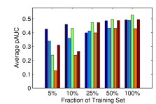
Refer to caption
(a) β=0.05𝛽0.05\beta=0.05
Refer to caption
(b) β=0.1𝛽0.1\beta=0.1
Refer to caption
Figure 4: Partial AUC maximization in [0,β]0𝛽[0,\beta] on PPI data.

Protein-protein interaction prediction. In protein-protein interaction (PPI) prediction, the task is to predict whether a given pair of proteins interact or not. Owing to the highly imbalanced nature of PPI data (e.g. only 1 in every 600 protein pairs in yeast are found to interact), the partial AUC in a small FPR range [0,β]0𝛽[0,\beta] has been advocated as an evaluation measure for this application [34]. We used the PPI data for Yeast from [34], which contains 2,865 protein pairs known to be interacting (positive) and a random set of 237,384 protein pairs assumed to be non-interacting (negative); each protein-pair is represented using 85 features.111111In the original data set in [34], each protein pair is represented by 162 features, but there were several missing features; we used a subset of 85 features that contained less than 25% missing values (with missing feature values replaced by mean/mode values). We evaluated the partial AUC performance of these methods on two FPR intervals [0,0.05]00.05[0,0.05] and [0,0.1]00.1[0,0.1]. To compare the methods for different training sample sizes, we report results in Figure 4 for varying fractions of the training set. As seen, the proposed method almost always yields higher partial AUC in the specified FPR intervals compared to the SVMAUCsubscriptSVMAUC\textup{{SVM}}_{\textup{{AUC}}} method for optimizing the full AUC, thus confirming its focus on a select portion of the ROC curve. Interestingly, the difference in performance is more pronounced for smaller training sample sizes, implying that when one has limited training data, it is more beneficial to use the data to directly optimize the partial AUC rather than to optimize the full AUC. Also, in most cases, the proposed method performs comparable to or better than the other baselines; the pAUCBoost and Greedy-Heuristic methods perform particularly poorly on smaller training samples due to the use of heuristics.  
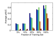
Refer to caption
(a) β=0.05𝛽0.05\beta=0.05
Refer to caption
(b) β=0.1𝛽0.1\beta=0.1
Refer to caption
Figure 5: Partial AUC maximization in [0,β]0𝛽[0,\beta] on drug discovery data.

Drug discovery. In the next task that we considered, one is given examples of chemical compounds that are active or inactive against a therapeutic target, and the goal is to rank new compounds such that the active ones are above the inactive ones. Here one is often interested in good ranking quality in the top portion of the ranked list, and hence good partial AUC in a small FPR interval [0,β]0𝛽[0,\beta] in the initial portion of the ROC curve is a performance measure of interest. In our experiments, we used a virtual screening data set from [20]; this contains 50 active/positive compounds (corresponding to the reversible antagonists of the α1Asubscript𝛼1A\alpha_{\text{1A}} adrenoceptor) and 2092 ones that are inactive/negative, with each compound represented as a 1021-bit vector using the FP2 molecular fingerprint representation (as done in [2]). Figure 5 contains the partial AUC performance for varying fractions of the training set on two FPR intervals. Clearly, for the most part, SVMpAUCsubscriptSVMpAUC\text{SVM}_{\text{pAUC}} yields higher partial AUC values than SVMAUCsubscriptSVMAUC\text{SVM}_{\text{AUC}}, and performs comparable to or better than the other baseline algorithms.

8.2 Maximizing Partial AUC in [α,β]𝛼𝛽[\alpha,\beta]

We next move to our experiments on partial AUC in a general [α,β]𝛼𝛽[\alpha,\beta] interval. We refer to the proposed structural SVM method for maximizing partial AUC in [α,β]𝛼𝛽[\alpha,\beta] again as SVMpAUCsubscriptSVMpAUC\textup{{SVM}}_{\textup{{pAUC}}} and our DC programming approach for optimizing the non-convex hinge surrogate as SVMpAUCdcsubscriptsuperscriptSVMdcpAUC\textup{{SVM}}^{\textup{{dc}}}_{\textup{{pAUC}}}. As baselines, we included SVMAUCsubscriptSVMAUC\textup{{SVM}}_{\textup{{AUC}}}, pAUCBoost which can optimize partial AUC over FPR ranges [α,β]𝛼𝛽[\alpha,\beta], and an extension of the greedy heuristic method in [37] to handle arbitrary FPR ranges. We first present our results on a real-world application, where partial AUC in [α,β]𝛼𝛽[\alpha,\beta] is a useful evaluation measure.

pAUC(0.2s,0.3s)pAUC0.2𝑠0.3𝑠\text{{pAUC}}(0.2s,0.3s)
SVMpAUC[0.2s,0.3s]subscriptSVMpAUC0.2𝑠0.3𝑠\text{SVM}_{\text{pAUC}}[0.2s,0.3s] 0.6376
SVMpAUCdc[0.2s,0.3s]subscriptsuperscriptSVMdcpAUC0.2𝑠0.3𝑠\text{SVM}^{\text{dc}}_{\text{pAUC}}[0.2s,0.3s] 0.6162
SVMAUCsubscriptSVMAUC\text{SVM}_{\text{AUC}} 0.6117
pAUCBoost[0.2s,0.3s]0.2𝑠0.3𝑠[0.2s,0.3s] 0.6033
Greedy-Heuristic[0.2s,0.3s]0.2𝑠0.3𝑠[0.2s,0.3s] 0.5616
Table 2: Partial AUC maximization in [α,β]𝛼𝛽[\alpha,\beta] with KDD Cup 08 data. Here s=6848/101671𝑠6848101671s=6848/101671.

Breast cancer detection. We consider the task stated in the KDD Cup 2008 challenge, where one is required to predict whether a given region of interest (ROI) from a breast X-ray image corresponds to a malignant (positive) or a benign (negative) tumor [36]. The data provided is collected from 118 malignant patients and 1,594 normal patients. Four X-ray images are available for each patient; overall, there are 102,294 candidate ROIs selected from these X-ray images, of which 623 are positive, with each ROI represented by 117 features. In the KDD Cup challenge, performance was evaluated in terms of the partial area under the free-response operating characteristic (FROC) curve in a false positive range [0.2,0.3]0.20.3[0.2,0.3] deemed clinically relevant based on radiologist surveys. The FROC curve [26] effectively uses a scaled version of the false positive rate in the usual ROC curve; for our purposes, the corresponding false positive rate is obtained by re-scaling by a factor of s=6848/101671𝑠6848101671s=6848/101671 (this is the total number of images divided by the total number of negative ROIs). Thus, the goal in our experiments was to maximize the partial AUC in the clinically relevant FPR range [0.2s,0.3s]0.2𝑠0.3𝑠[0.2s,0.3s]. Table 2 presents results on algorithms SVMpAUCsubscriptSVMpAUC\textup{{SVM}}_{\textup{{pAUC}}} and SVMpAUCdcsubscriptsuperscriptSVMdcpAUC\textup{{SVM}}^{\textup{{dc}}}_{\textup{{pAUC}}} developed for FPR intervals of this form, as well as on the baseline methods; SVMpAUCsubscriptSVMpAUC\textup{{SVM}}_{\textup{{pAUC}}} performs the best in this case.

Data set #instances #features
a9a 48,842 123
cod-rna 488,565 8
covtype 581,012 54
ijcnn1 141,691 22
letter 20,000 16
Table 3: UCI data sets used.
pAUC(0.02,0.05)pAUC0.020.05\text{{pAUC}}(0.02,0.05)
a9a cod-rna covtype ijcnn1 letter
SVMpAUCsubscriptSVMpAUC\text{SVM}_{\text{pAUC}} [0.02, 0.05] 0.2739 0.9187 0.2467 0.6131 0.5208
SVMpAUCdcsubscriptsuperscriptSVMdcpAUC\text{SVM}^{\text{dc}}_{\text{pAUC}} [0.02, 0.05] 0.3650 0.9196 0.2410 0.6798 0.5182
SVMAUCsubscriptSVMAUC\text{SVM}_{\text{AUC}} 0.4338 0.9192 0.2987 0.4750 0.4455
pAUCBooost [0.02, 0.05] 0.4012 0.0330 0.4485 0.4913 0.4954
GreedyHeuristic[0.02, 0.05] 0.3417 0.0329 0.2386 0.1201 0.2888
Table 4: Partial AUC maximization in [0.02, 0.05] on UCI data sets.

UCI data sets. To perform a more detailed comparison between the proposed structural SVM and DC programming methods for general [α,β]𝛼𝛽[\alpha,\beta] intervals, we also evaluated the methods on a number of benchmark data sets obtained from the UCI machine learning repository [12] (see Table 3). The results for the FPR interval [0.02,0.05]0.020.05[0.02,0.05] are shown in Table 4; for completeness, we also report the performance of the baseline methods. Despite having to solve a non-convex optimization problem (and hence running the risk of getting stuck at a locally optimum solution), SVMpAUCdcsubscriptsuperscriptSVMdcpAUC\textup{{SVM}}^{\textup{{dc}}}_{\textup{{pAUC}}} does perform better than SVMpAUCsubscriptSVMpAUC\textup{{SVM}}_{\textup{{pAUC}}} in some cases, though between the two, there is no clear winner. Also, on three of the five data sets, one of the two proposed methods yield the best overall performance. The strikingly poor performance of pAUCBoost and Greedy-Heuristic on the cod-rna data set is because the features in this data set individually produce low partial AUC values; since these methods rely on local greedy heuristics, they fail to find a linear combination of the features that yields high partial AUC performance.

8.3 Maximizing TPR at a Specific FPR Value

We have so far seen that the proposed methods are good at learning scoring functions that yield high partial AUC in a specified FPR range. In our next experiment, we shall demonstrate that the proposed methods can also be useful in applications where one is required to learn a classifier with specific true/false positive requirements. In particular, we consider the task described in the KDD Cup 2006 challenge of detecting pulmonary emboli in medical images obtained from CT angiography [24]. Given a candidate region of interest (ROI) from the image, the goal is to predict whether it is a pulmonary emboli or not; a specific requirement here is that the classifier must have high TPR, with the FPR kept within a specified limit.

Indeed if a classifier is constructed by thresholding a scoring function, the above evaluation measure can be seen as the partial AUC of the scoring function in an infinitesimally small FPR interval. However, given the small size of the FPR interval concerned, maximizing this evaluation measure directly may not produce a classifier with good generalization performance, particularly with smaller training samples (see generalization bound in Section 7). Instead, we prescribe a more robust approach of using the methods developed in this paper to maximize partial AUC in an appropriate larger FPR interval, and constructing a classifier by suitably thresholding the scoring function thus obtained.

TPR at FPR =0.1absent0.1=0.1
SVMpAUC[0,0.1]subscriptSVMpAUC00.1\text{SVM}_{\text{pAUC}}[0,0.1] 0.6131
SVMpAUC[0.05,0.1]subscriptSVMpAUC0.050.1\text{SVM}_{\text{pAUC}}[0.05,0.1] 0.5839
SVMpAUCdc[0.05,0.1]subscriptsuperscriptSVMdcpAUC0.050.1\text{SVM}^{\text{dc}}_{\text{pAUC}}[0.05,0.1] 0.5912
SVMAUCsubscriptSVMAUC\text{SVM}_{\text{AUC}} 0.5839
Table 5: Partial AUC maximization as a proxy for maximizing the TPR at a specified FPR on KDD Cup 06 data.
Refer to caption
Refer to caption
(a) ppi
Refer to caption
Refer to caption
(b) ijcnn1
Figure 6: Partial AUC maximization in [0,β]0𝛽[0,\beta]: Comparison of average training and validation times between SVMpAUCsubscriptSVMpAUC\textup{{SVM}}_{\textup{{pAUC}}} and baseline methods.
Refer to caption
Refer to caption
(a) kddcup08
Refer to caption
Refer to caption
(b) ijcnn1
Figure 7: Partial AUC maximization in [α,β]𝛼𝛽[\alpha,\beta]: Comparison of average training and validation times between SVMpAUCsubscriptSVMpAUC\textup{{SVM}}_{\textup{{pAUC}}}, SVMpAUCdcsubscriptsuperscriptSVMdcpAUC\textup{{SVM}}^{\textup{{dc}}}_{\textup{{pAUC}}} and baseline methods. Here s=6848/101671𝑠6848101671s=6848/101671.

The data provided in the KDD Cup challenge consists of 4,429 ROIs represented with 116 features, of which 500 are positive. We considered a maximum allowable FPR limit of 0.10.10.1 (which is one of the values prescribed in the challenge). The proposed partial AUC maximization methods were used to learn scoring functions for two FPR intervals, [0,0.1]00.1[0,0.1] and [0.05,0.1]0.050.1[0.05,0.1], that we expected will promote high TPR at the given FPR of 0.1; the performance of a learned model was then evaluated based on the TPR it yields when thresholded at a FPR of 0.1. Table 5 contains results for SVMpAUCsubscriptSVMpAUC\textup{{SVM}}_{\textup{{pAUC}}} on both intervals, and for SVMpAUCdcsubscriptsuperscriptSVMdcpAUC\textup{{SVM}}^{\textup{{dc}}}_{\textup{{pAUC}}} on the [0.05,0.1]0.050.1[0.05,0.1] interval. We also included SVMAUCsubscriptSVMAUC\textup{{SVM}}_{\textup{{AUC}}} for comparison. Interestingly, in this case, SVMpAUCsubscriptSVMpAUC\textup{{SVM}}_{\textup{{pAUC}}} in [0,0.1]00.1[0,0.1] performs the best; the DC programming method on the [0.05,0.1]0.050.1[0.05,0.1] interval comes a close second, performing better than the structural SVM approach for the same interval.121212The experiments were carried out on a single 70%-30% train-test split provided in the challenge.

We also note that in a follow-up work, the proposed approach was applied to a similar problem in personalized cancer treatment [25], where the goal was to predict whether a given cancer patient will respond well to a drug treatment. In this application, one again requires high true positive rates (fraction of cases where the treatment is effective and the model predicts the same), subject to the false positive rate being within an allowable limit; as above, the problem was posed as a partial AUC maximization task, and the classifiers learned using our methods were found to yield higher TPR performance than standard approaches for this problem, while not exceeding the allowed FPR limit.

8.4 Run-time Analysis
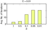
Refer to caption
Refer to caption
Refer to caption
(a) ppi
Refer to caption
Refer to caption
Refer to caption
(b) covtype
Refer to caption
Refer to caption
Refer to caption
(c) ijcnn1
Figure 8: Partial AUC in [0,β]0𝛽[0,\beta]: Average number of cutting plane iterations in SVMpAUCsubscriptSVMpAUC\textup{{SVM}}_{\textup{{pAUC}}} vs. length of FPR interval for different values of regularization parameter C𝐶C. Here β=1𝛽1\beta=1 corresponds to the full AUC optimizing method SVMAUCsubscriptSVMAUC\textup{{SVM}}_{\textup{{AUC}}}.
Refer to caption
Refer to caption
Refer to caption
Figure 9: Partial AUC in [α,β]𝛼𝛽[\alpha,\beta] on KDD Cup 08 data: Average number of cutting plane iterations in SVMpAUCsubscriptSVMpAUC\textup{{SVM}}_{\textup{{pAUC}}} vs. length of FPR interval for different values of α𝛼\alpha.

Run-time comparison with baseline methods. In our final set of experiments, we compared the running times of the various algorithms evaluated above. Figure 7 contains the average training times (across five train-test splits) for partial AUC maximization tasks involving [0,β]0𝛽[0,\beta] FPR intervals on two data sets. We also report the time take for validation/parameter tuning in SVMpAUCsubscriptSVMpAUC\textup{{SVM}}_{\textup{{pAUC}}}, SVMAUCsubscriptSVMAUC\textup{{SVM}}_{\textup{{AUC}}} and ASVM; the remaining two methods do not have tunable parameters. The running times for partial AUC maximization in a general [α,β]𝛼𝛽[\alpha,\beta] range is shown in Figure 7 for two data sets. All experiments were run on an Intel Xeon (2.13 GHz) machine with 12 GB RAM.

Notice that except for SVMAUCsubscriptSVMAUC\textup{{SVM}}_{\textup{{AUC}}}, all the baselines require higher or similar training times compared to SVMpAUCsubscriptSVMpAUC\textup{{SVM}}_{\textup{{pAUC}}}. Also, as expected, for the [α,β]𝛼𝛽[\alpha,\beta] intervals, the DC programming based SVMpAUCdcsubscriptsuperscriptSVMdcpAUC\textup{{SVM}}^{\textup{{dc}}}_{\textup{{pAUC}}} (which solves an entire structural SVM problem in each iteration) requires higher training time than SVMpAUCsubscriptSVMpAUC\textup{{SVM}}_{\textup{{pAUC}}}. The reason for the full AUC maximizing SVMAUCsubscriptSVMAUC\textup{{SVM}}_{\textup{{AUC}}} method being the fastest in all cases, despite the subroutine for finding the most-violated constraint requiring higher computational time compared to that for partial AUC, is because the number of iterations required by the cutting plane solver is lower for AUC. This will become clear in our next experiments where we report the number of iterations taken by the cutting plane solver under different settings.  

Influence of α𝛼\alpha, β𝛽\beta and C𝐶C on number of cutting plane iterations. We next analysed the number of iterations taken by the cutting plane method in SVMAUCsubscriptSVMAUC\textup{{SVM}}_{\textup{{AUC}}} and SVMpAUCsubscriptSVMpAUC\textup{{SVM}}_{\textup{{pAUC}}}, i.e. the number of calls made to the routine for finding the most violated constraint (Algorithms 2 and 3), for different FPR intervals and regularization parameter values. Our results for FPR ranges of the form [0,β]0𝛽[0,\beta] are shown in Figure 8, where we provide plots of the average number of cutting plane iterations (over five train-test splits) as a function of β𝛽\beta for different values of the regularization parameter C𝐶C. It is often seen that the number of iterations of the cutting plane method increases as β𝛽\beta decreases (i.e. as the FPR interval becomes smaller), suggesting that optimizing partial AUC is harder for smaller intervals; this explains why the overall training time is lower for maximizing the full AUC (i.e. for SVMAUCsubscriptSVMAUC\textup{{SVM}}_{\textup{{AUC}}}) compared to the time taken for maximizing partial AUC in a small interval. Similarly, the number of cutting plane iterations increases with C𝐶C, as suggested by the method’s convergence rate (see Section 4).

Our results for general FPR intervals [α,β]𝛼𝛽[\alpha,\beta] are shown in Figure 9, where we have plots of the average number of cutting plane iterations as a function of the interval length, for different values of α𝛼\alpha. Again, it is seen that the number of iterations is higher for smaller FPR intervals; interestingly, the number of iterations also increases as the interval is farther away to the right.

9 Conclusion and Open Questions

The partial AUC is increasingly used as a performance measure in several machine learning and data mining applications. We have developed support vector algorithms for optimizing the partial AUC between two given false positive rates α𝛼\alpha and β𝛽\beta. Unlike the full AUC, where it is straightforward to develop surrogate optimizing methods, even constructing a (tight) convex surrogate for the partial AUC turns out to be non-trivial. By exploiting the specific structure of the evaluation measure and extending the structural SVM framework of [18], we have constructed convex surrogates for the partial AUC, and developed an efficient cutting plane method for solving the resulting optimization problem. In addition, we have also provided a DC programming method for optimizing a non-convex hinge surrogate that is tighter for general false positive ranges [α,β]𝛼𝛽[\alpha,\beta]. Our empirical evaluations on several real-world and benchmark tasks indicate that the proposed methods do indeed optimize the partial AUC in the desired false positive range, often performing comparable to or better than existing baseline techniques.

Subsequent to the conference versions of this paper, there have been a number of follow-up works. As noted earlier, one such work applied our algorithm to an important problem in personalized cancer treatment [25], where the task was to predict clinical responses of patients to chemotherapy. Other works include minibatch extensions of our structural SVM method for the [0,β]0𝛽[0,\beta] range to online and large scale stochastic settings [21], as well as an ensemble style version of this method with application to a problem in computer vision [31, 32]

There are several questions that remain open. Firstly, we observed in our experiments that the number of iterations required by the proposed cutting plane solvers to converge depends on the length of the specified FPR range, but this is not evident from the current convergence rate for the solver (see Section 4) obtained from a result in [19]. It would be of interest to see if tighter convergence rates that match our empirical observation can be shown for the cutting plane solver. Secondly, it would be useful to understand the consistency properties of the proposed algorithms. Such studies exist for methods that optimize the full AUC and more recently, for other complex performance measures for classification such as the F-measure [23, 28, 27], but these results do not extend directly to the methods in this paper. Finally, one could look at extensions of the proposed algorithms to multiclass classification and ordinal regression settings, where often there are different constraints on the error rates of a predictor on different classes. Again, there has been work on optimizing multiclass versions of the full AUC [43, 7, 42], and similar methods for multiclass variants of the partial AUC will be useful to have.

Acknowledgments

HN thanks Prateek Jain and Purushottam Kar for helpful discussions. HN also thanks Purushottam Kar for providing preprocessed versions of some of the data sets and a wrapper code for the experiments, and for an email correspondence that led us to identify an error in the version of Theorem 7 that appeared in a conference version of this paper [30]; the error has been corrected here. This work was done when HN was a PhD student at the Indian Institute of Science, Bangalore and was supported by a Google India PhD Fellowship. SA thanks DST for support under a Ramanujan Fellowship.

References

  • [1] S. Agarwal. The Infinite Push: A new support vector ranking algorithm that directly optimizes accuracy at the absolute top of the list. In SDM, 2011.
  • [2] S. Agarwal, D. Dugar, and S. Sengupta. Ranking chemical structures for drug discovery: A new machine learning approach. Journal of Chemical Information and Modeling, 50(5):716–731, 2010.
  • [3] S. Agarwal, T. Graepel, R. Herbrich, S. Har-Peled, and D. Roth. Generalization bounds for the area under the ROC curve. Journal of Machine Learning Research, 6:393–425, 2005.
  • [4] D. P. Bertsekas. Nonlinear Programming. Athena Scientific, Belmont, MA, 1999.
  • [5] C. Burges, T. Shaked, E. Renshaw, A. Lazier, M. Deeds, N. Hamilton, and G. Hullender. Learning to rank using gradient descent. In ICML, 2005.
  • [6] Wei Chu and S Sathiya Keerthi. Support vector ordinal regression. Neural computation, 19(3):792–815, 2007.
  • [7] S. Clémençon, S. Robbiano, and N. Vayatis. Ranking data with ordinal labels: Optimality and pairwise aggregation. Machine learning, 91(1):67–104, 2013.
  • [8] C. Cortes and M. Mohri. AUC optimization vs. error rate minimization. In NIPS, 2004.
  • [9] Corinna Cortes and Vladimir Vapnik. Support-vector networks. Machine learning, 20(3):273–297, 1995.
  • [10] Koby Crammer and Yoram Singer. On the algorithmic implementation of multiclass kernel-based vector machines. Journal of Machine Learning Research, 2:265–292, 2002.
  • [11] L. E. Dodd and M. S. Pepe. Partial AUC estimation and regression. Biometrics, 59(3):614–623, 2003.
  • [12] A. Frank and Arthur Asuncion. UCI machine learning repository. url: http://archive.ics.uci.edu/ml, 2010.
  • [13] Y. Freund, R. Iyer, R. E. Schapire, and Y. Singer. An efficient boosting algorithm for combining preferences. Journal of Machine Learning Research, 4:933–969, 2003.
  • [14] R. Herbrich, T. Graepel, and K. Obermayer. Large margin rank boundaries for ordinal regression. In A. Smola, P. Bartlett, B. Schoelkopf, and D. Schuurmans, editors, Advances in Large Margin Classifiers, pages 115–132. 2000.
  • [15] M.-J. Hsu and H.-M. Hsueh. The linear combinations of biomarkers which maximize the partial area under the ROC curve. Computational Statistics, pages 1–20, 2012.
  • [16] Man-Jen Hsu, Yuan-Chin I Chang, and Huey-Miin Hsueh. Biomarker selection for medical diagnosis using the partial area under the ROC curve. BMC research notes, 7(1):25, 2014.
  • [17] T. Joachims. Optimizing search engines using clickthrough data. In ICML, 2002.
  • [18] T. Joachims. A support vector method for multivariate performance measures. In ICML, 2005.
  • [19] T. Joachims. Training linear SVMs in linear time. In KDD, 2006.
  • [20] R. N. Jorissen and M. K. Gilson. Virtual screening of molecular databases using a support vector machine. Journal of Chemical Information and Modeling, 45:549–561, 2005.
  • [21] Purushottam Kar, Harikrishna Narasimhan, and Prateek Jain. Online and stochastic gradient methods for non-decomposable loss functions. In NIPS, 2014.
  • [22] O. Komori and S. Eguchi. A boosting method for maximizing the partial area under the ROC curve. BMC Bioinformatics, 11:314, 2010.
  • [23] O. Koyejo, N. Natarajan, P. Ravikumar, and I.S. Dhillon. Consistent binary classification with generalized performance metrics. In NIPS, 2014.
  • [24] Terran Lane, Bharat Rao, Jinbo Bi, Jianming Liang, and Marcos Salganicoff. On the medical frontier: the 2006 kdd cup competition and results. SIGKDD Explor. Newsletter, 8(2):39–46, 2006.
  • [25] Biswanath Majumder, Ulaganathan Baraneedharan, Saravanan Thiyagarajan, Padhma Radhakrishnan, Harikrishna Narasimhan, Muthu Dhandapani, Nilesh Brijwani, Dency D Pinto, Arun Prasath, Basavaraja U Shanthappa, et al. Predicting clinical response to anticancer drugs using an ex vivo platform that captures tumour heterogeneity. Nature communications, 6, 2015.
  • [26] H. Miller. The FROC curve: A representation of the observer’s performance for the method of free response. Journal of the Acoustical Society of America, 46(6B):1473–1476, 1969.
  • [27] H. Narasimhan, H.G. Ramaswamy, A. Saha, and S. Agarwal. Consistent multiclass algorithms for complex performance measures. In ICML, 2015.
  • [28] H. Narasimhan, R. Vaish, and S. Agarwal. On the statistical consistency of plug-in classifiers for non-decomposable performance measures. In NIPS, 2014.
  • [29] Harikrishna Narasimhan and Shivani Agarwal. A structural SVM based approach for optimizing partial AUC. In ICML, 2013.
  • [30] Harikrishna Narasimhan and Shivani Agarwal. SVMtightpAUCsuperscriptsubscriptabsentpAUCtight{}_{\text{{pAUC}}}^{\text{tight}}: A new support vector method for optimizing partial AUC based on a tight convex upper bound. In KDD, 2013.
  • [31] Sakrapee Paisitkriangkrai, Chunhua Shen, and Anton Van Den Hengel. Efficient pedestrian detection by directly optimizing the partial area under the ROC curve. In ICCV, 2013.
  • [32] Sakrapee Paisitkriangkrai, Chunhua Shen, and Anton van den Hengel. Strengthening the effectiveness of pedestrian detection with spatially pooled features. In ECCV, 2014.
  • [33] M. S. Pepe and M. L. Thompson. Combining diagnostic test results to increase accuracy. Biostatistics, 1(2):123–140, 2000.
  • [34] Y. Qi, Z. Bar-Joseph, and J. Klein-seetharaman. Evaluation of different biological data and computational classification methods for use in protein interaction prediction. Proteins, 63:490–500, 2006.
  • [35] A Rakotomamonjy. Sparse support vector infinite push. In ICML, 2012.
  • [36] R. B. Rao, O. Yakhnenko, and B. Krishnapuram. KDD Cup 2008 and the workshop on mining medical data. SIGKDD Explor. Newsletter, 10(2):34–38, 2008.
  • [37] M. T. Ricamato and F. Tortorella. Partial AUC maximization in a linear combination of dichotomizers. Pattern Recognition, 44(10-11):2669–2677, 2011.
  • [38] C. Rudin. The p-norm push: A simple convex ranking algorithm that concentrates at the top of the list. Journal of Machine Learning Research, 10:2233–2271, 2009.
  • [39] Matthew J Schneider and Wilpen L Gorr. ROC-based model estimation for forecasting large changes in demand. International Journal of Forecasting, 31(2):253–262, 2015.
  • [40] T. Takenouchi, O. Komori, and S. Eguchi. An extension of the receiver operating characteristic curve and AUC-optimal classification. Neural Computation, 24(10):2789–2824, 2012.
  • [41] I. Tsochantaridis, T. Joachims, T. Hofmann, and Y. Altun. Large margin methods for structured and interdependent output variables. Journal of Machine Learning Research, 6:1453–1484, 2005.
  • [42] Kazuki Uematsu and Yoonkyung Lee. Statistical optimality in multipartite ranking and ordinal regression. IEEE Transactions on Pattern Analysis and Machine Intelligence, 37(5):1080–1094, 2015.
  • [43] W. Waegeman, B. De Baets, and L. Boullart. Learning layered ranking functions with structured support vector machines. Neural Networks, 21(10):1511–1523, 2008.
  • [44] Z. Wang and Y.-C.I. Chang. Marker selection via maximizing the partial area under the ROC curve of linear risk scores. Biostatistics, 12(2):369–385, 2011.
  • [45] S.-H. Wu, K.-P. Lin, C.-M. Chen, and M.-S. Chen. Asymmetric support vector machines: low false-positive learning under the user tolerance. In KDD, 2008.
  • [46] C. J. Yu and T. Joachims. Training structural SVMs with kernels using sampled cuts. In KDD, 2008.
  • [47] Chun-Nam John Yu and Thorsten Joachims. Learning structural SVMs with latent variables. In ICML, 2009.
  • [48] Y. Yue, T. Finley, F. Radlinski, and T. Joachims. A support vector method for optimizing average precision. In SIGIR, 2007.
  • [49] Alan L Yuille and Anand Rangarajan. The concave-convex procedure (CCCP). Neural Computation, 15(4):915–936, 2003.

Appendix A Proofs

A.1 Proof of Theorem 1

Proof.

We simplify the structural SVM surrogate into a pair-wise form:

R^AUCstruct(w;S)subscriptsuperscript^𝑅structAUC𝑤𝑆\displaystyle\widehat{R}^{\textup{{struct}}}_{\textup{{AUC}}}(w;\,S) =\displaystyle= maxπΠm,n{ΔAUC(π,π)(wϕ(S,π)wϕ(S,π))}𝜋subscriptΠ𝑚𝑛subscriptΔAUCsuperscript𝜋𝜋superscript𝑤topitalic-ϕ𝑆superscript𝜋superscript𝑤topitalic-ϕ𝑆𝜋\displaystyle\underset{\pi\,\in\,\Pi_{m,n}}{\max}\big{\{}\Delta_{\textup{{AUC}}}(\pi^{*},\pi)\,-\,(w^{\top}\phi(S,\pi^{*})-w^{\top}\phi(S,\pi))\big{\}}
=\displaystyle= maxπΠm,n{1mni=1mj=1nπij(1w(xi+xj))}.𝜋subscriptΠ𝑚𝑛max1𝑚𝑛superscriptsubscript𝑖1𝑚superscriptsubscript𝑗1𝑛subscript𝜋𝑖𝑗1superscript𝑤topsubscriptsuperscript𝑥𝑖subscriptsuperscript𝑥𝑗\displaystyle\underset{\pi\,\in\,\Pi_{m,n}}{\operatorname{max}}\bigg{\{}\frac{1}{mn}\sum_{i=1}^{m}\sum_{j=1}^{n}\pi_{ij}\big{(}1\,-\,w^{\top}(x^{+}_{i}-x^{-}_{j})\big{)}\bigg{\}}.

Now consider solving a relaxed form of the above argmax over all matrices in {0,1}m×nsuperscript01𝑚𝑛\{0,1\}^{m\times n}. Since the objective is linear in the individual entries of πijsubscript𝜋𝑖𝑗\pi_{ij}, each πijsubscript𝜋𝑖𝑗\pi_{ij} can be optimized independently, giving us

maxπ{0,1}m×n1mni=1mj=1nπij(1w(xi+xj))𝜋superscript01𝑚𝑛1𝑚𝑛superscriptsubscript𝑖1𝑚superscriptsubscript𝑗1𝑛subscript𝜋𝑖𝑗1superscript𝑤topsubscriptsuperscript𝑥𝑖subscriptsuperscript𝑥𝑗\displaystyle\underset{\pi\,\in\,\{0,1\}^{m\times n}}{\max}\,\frac{1}{mn}\sum_{i=1}^{m}\sum_{j=1}^{n}\pi_{ij}\big{(}1\,-\,w^{\top}(x^{+}_{i}-x^{-}_{j})\big{)}
=\displaystyle= 1mni=1mj=1nmaxπij{0,1}πij(1w(xi+xj))1𝑚𝑛superscriptsubscript𝑖1𝑚superscriptsubscript𝑗1𝑛subscript𝜋𝑖𝑗01subscript𝜋𝑖𝑗1superscript𝑤topsubscriptsuperscript𝑥𝑖subscriptsuperscript𝑥𝑗\displaystyle\frac{1}{mn}\sum_{i=1}^{m}\sum_{j=1}^{n}\underset{\pi_{ij}\,\in\,\{0,1\}}{\max}\pi_{ij}\big{(}1\,-\,w^{\top}(x^{+}_{i}-x^{-}_{j})\big{)}\hskip 56.9055pt
=\displaystyle= 1mni=1mj=1nπ¯ij(1w(xi+xj)),1𝑚𝑛superscriptsubscript𝑖1𝑚superscriptsubscript𝑗1𝑛subscript¯𝜋𝑖𝑗1superscript𝑤topsubscriptsuperscript𝑥𝑖subscriptsuperscript𝑥𝑗\displaystyle\frac{1}{mn}\sum_{i=1}^{m}\sum_{j=1}^{n}\bar{\pi}_{ij}\big{(}1\,-\,w^{\top}(x^{+}_{i}-x^{-}_{j})\big{)},

where π¯ij=𝟏(w(xi+xj)1)subscript¯𝜋𝑖𝑗1superscript𝑤topsubscriptsuperscript𝑥𝑖subscriptsuperscript𝑥𝑗1\bar{\pi}_{ij}={\mathbf{1}}\big{(}w^{\top}(x^{+}_{i}-x^{-}_{j})\leq 1\big{)}. It can be seen that this optimal matrix π¯¯𝜋\bar{\pi} is in fact a valid ordering matrix in Πm,nsubscriptΠ𝑚𝑛\Pi_{m,n}, as it corresponds to ordering of instances where the positives are scored according to wxsuperscript𝑤top𝑥w^{\top}x and the negatives are scored according to wx+1superscript𝑤top𝑥1w^{\top}x+1. Thus π¯¯𝜋\bar{\pi} is also a solution to the original unrelaxed problem and hence

R^AUCstruct(w;S)subscriptsuperscript^𝑅structAUC𝑤𝑆\displaystyle\widehat{R}^{\textup{{struct}}}_{\textup{{AUC}}}(w;\,S) =\displaystyle= 1mni=1mj=1nπ¯ij(1w(xi+xj))1𝑚𝑛superscriptsubscript𝑖1𝑚superscriptsubscript𝑗1𝑛subscript¯𝜋𝑖𝑗1superscript𝑤topsubscriptsuperscript𝑥𝑖subscriptsuperscript𝑥𝑗\displaystyle\frac{1}{mn}\sum_{i=1}^{m}\sum_{j=1}^{n}\bar{\pi}_{ij}\big{(}1\,-\,w^{\top}(x^{+}_{i}-x^{-}_{j})\big{)}
=\displaystyle= 1mni=1mj=1n(1w(xi+xj))+1𝑚𝑛superscriptsubscript𝑖1𝑚superscriptsubscript𝑗1𝑛subscript1superscript𝑤topsubscriptsuperscript𝑥𝑖subscriptsuperscript𝑥𝑗\displaystyle\frac{1}{mn}\sum_{i=1}^{m}\sum_{j=1}^{n}\big{(}1\,-\,w^{\top}(x^{+}_{i}-x^{-}_{j})\big{)}_{+}
=\displaystyle= R^AUChinge(w;S),as desired.subscriptsuperscript^𝑅hingeAUC𝑤𝑆as desired.\displaystyle\widehat{R}^{\textup{{hinge}}}_{\textup{{AUC}}}(w;\,S),~{}~{}\text{as desired.}

A.2 Proof of Theorem 2

We begin with some intuition. Suppose the given FPR range is [n1n,1]𝑛1𝑛1\displaystyle\bigg{[}\frac{n-1}{n},1\bigg{]} where jα=n1>0subscript𝑗𝛼𝑛10j_{\alpha}=n-1>0 and jβ=nsubscript𝑗𝛽𝑛j_{\beta}=n, the hinge surrogate reduces to a ‘min’ of convex functions in w𝑤w and it is easy to see that there are training samples S𝑆S where the surrogate is non-convex in w𝑤w. The same argument can be extended to general kthsuperscript𝑘thk^{\text{th}} order statistic of a set of convex functions in w𝑤w when k>1𝑘1k>1, and as seen below to general FPR intervals.

In particular, for any given FPR range [α,β]𝛼𝛽[\alpha,\beta] with α>0𝛼0\alpha>0, we provide a two-dimensional training sample S=(S+,S)𝑆subscript𝑆subscript𝑆S=(S_{+},S_{-}) with m=1𝑚1m=1 positive instance and n𝑛n negative instances, for which the hinge surrogate R^pAUChinge(α,β)(w;S)subscriptsuperscript^𝑅hingepAUC𝛼𝛽𝑤𝑆\widehat{R}^{\textup{{hinge}}}_{\textup{{pAUC}}}(\alpha,\beta)(w;S) (in Eq. (9)) is non-convex in w𝑤w. The training sample is constructed as follows: S+=(x1+=(0,0))2subscript𝑆superscriptsubscript𝑥1superscript00topsuperscript2S_{+}=(x_{1}^{+}=(0,0)^{\top})\in{\mathbb{R}}^{2} and S=(x1,,xn)(2)nsubscript𝑆subscriptsuperscript𝑥1subscriptsuperscript𝑥𝑛superscriptsuperscript2𝑛S_{-}=(x^{-}_{1},\ldots,x^{-}_{n})\in({\mathbb{R}}^{2})^{n}, with

xj={(0,1)if j=1(0,0)if j{2,,jα}(1,0)if j=jα+1(1,1)otherwise.subscriptsuperscript𝑥𝑗casessuperscript01topif 𝑗1superscript00topif 𝑗2subscript𝑗𝛼superscript10topif 𝑗subscript𝑗𝛼1superscript11topotherwisex^{-}_{j}=\begin{cases}(0,-1)^{\top}&\text{if }j=1\\ (0,0)^{\top}&\text{if }j\in\{2,\ldots,j_{\alpha}\}\\ (-1,0)^{\top}&\text{if }j=j_{\alpha}+1\\ (-1,-1)^{\top}&\text{otherwise}\end{cases}.

The corresponding hinge surrogate for a linear model w2𝑤superscript2w\in{\mathbb{R}}^{2} is given by:

R^pAUC(α,β)hinge(w;S)subscriptsuperscript^𝑅hingepAUC𝛼𝛽𝑤𝑆\displaystyle\widehat{R}^{\textup{{hinge}}}_{\textup{{pAUC}}(\alpha,\beta)}(w;S) =\displaystyle= 1m(jβjα)i=1mj=jα+1jβ(1+w(x(j)wxi+))+1𝑚subscript𝑗𝛽subscript𝑗𝛼superscriptsubscript𝑖1𝑚superscriptsubscript𝑗subscript𝑗𝛼1subscript𝑗𝛽subscript1superscript𝑤topsuperscriptsubscript𝑥subscript𝑗𝑤superscriptsubscript𝑥𝑖\displaystyle\frac{1}{m(j_{\beta}-j_{\alpha})}\sum_{i=1}^{m}\sum_{j=j_{\alpha}+1}^{j_{\beta}}\big{(}1\,+\,w^{\top}(x_{(j)_{w}}^{-}\,-\,x_{i}^{+})\big{)}_{+}
=\displaystyle= 1jβjαj=jα+1jβ(1+w(x(j)w))+.1subscript𝑗𝛽subscript𝑗𝛼superscriptsubscript𝑗subscript𝑗𝛼1subscript𝑗𝛽subscript1superscript𝑤topsuperscriptsubscript𝑥subscript𝑗𝑤\displaystyle\frac{1}{j_{\beta}-j_{\alpha}}\sum_{j=j_{\alpha}+1}^{j_{\beta}}\big{(}1\,+\,w^{\top}(x_{(j)_{w}}^{-})\big{)}_{+}.

For simplicity let us refer to the above surrogate function in the specified FPR interval using the shorthand R^(w)^𝑅𝑤\widehat{R}(w). To show that the surrogate is non-convex in w𝑤w, we will now identify linear models w1,w22subscript𝑤1subscript𝑤2superscript2w_{1},w_{2}\in{\mathbb{R}}^{2} such that: R^(0.5w1+0.5w2)>0.5R^(w1)+ 0.5R^(w2).^𝑅0.5subscript𝑤10.5subscript𝑤20.5^𝑅subscript𝑤10.5^𝑅subscript𝑤2\widehat{R}(0.5\,w_{1}+0.5\,w_{2})>0.5\,\widehat{R}(w_{1})\,+\,0.5\,\widehat{R}(w_{2}). Let w1=(1,0)2subscript𝑤1superscript10topsuperscript2w_{1}=(1,0)^{\top}\in{\mathbb{R}}^{2} and w2=(0,1)2subscript𝑤2superscript01topsuperscript2w_{2}=(0,1)^{\top}\in{\mathbb{R}}^{2}, and denote w3=0.5w1+0.5w2=(0.5,0.5)subscript𝑤30.5subscript𝑤10.5subscript𝑤2superscript0.50.5topw_{3}=0.5\,w_{1}+0.5\,w_{2}=(0.5,0.5)^{\top}, a convex combination of these models. Note that w1subscript𝑤1w_{1} ranks the instances using the first feature, with all negative instances ranked in positions jα+1subscript𝑗𝛼1j_{\alpha}+1 to jβsubscript𝑗𝛽j_{\beta} given a score of 11-1; the model w2subscript𝑤2w_{2} ranks the instances using the second feature, with all negative instances ranked in positions jα+1subscript𝑗𝛼1j_{\alpha}+1 to jβsubscript𝑗𝛽j_{\beta} again given a score of 11-1; the model w3subscript𝑤3w_{3} ranks instances using a convex combination of the features, and in this case, the negative instance ranked in position jα+1subscript𝑗𝛼1j_{\alpha}+1 gets a score of 0.50.5-0.5, while those in positions jα+2subscript𝑗𝛼2j_{\alpha}+2 to jβsubscript𝑗𝛽j_{\beta} get a score of 11-1. The surrogate then evaluates to the following values for these models:

R^(w1)=1jβjαj=jα+1jβ(1+w1x(j)w1)+=1jβjαj=jα+1jβ(11)+= 0^𝑅subscript𝑤11subscript𝑗𝛽subscript𝑗𝛼superscriptsubscript𝑗subscript𝑗𝛼1subscript𝑗𝛽subscript1superscriptsubscript𝑤1topsuperscriptsubscript𝑥subscript𝑗subscript𝑤11subscript𝑗𝛽subscript𝑗𝛼superscriptsubscript𝑗subscript𝑗𝛼1subscript𝑗𝛽subscript11 0\displaystyle\widehat{R}(w_{1})\,=\,\frac{1}{j_{\beta}-j_{\alpha}}\sum_{j=j_{\alpha}+1}^{j_{\beta}}\big{(}1\,+\,w_{1}^{\top}x_{(j)_{w_{1}}}^{-}\big{)}_{+}\,=\,\frac{1}{j_{\beta}-j_{\alpha}}\sum_{j=j_{\alpha}+1}^{j_{\beta}}(1-1)_{+}\,=\,0
R^(w2)=1jβjαj=jα+1jβ(1+w1x(j)w1)+=1jβjαj=jα+1jβ(11)+= 0^𝑅subscript𝑤21subscript𝑗𝛽subscript𝑗𝛼superscriptsubscript𝑗subscript𝑗𝛼1subscript𝑗𝛽subscript1superscriptsubscript𝑤1topsuperscriptsubscript𝑥subscript𝑗subscript𝑤11subscript𝑗𝛽subscript𝑗𝛼superscriptsubscript𝑗subscript𝑗𝛼1subscript𝑗𝛽subscript11 0\displaystyle\widehat{R}(w_{2})\,=\,\frac{1}{j_{\beta}-j_{\alpha}}\sum_{j=j_{\alpha}+1}^{j_{\beta}}\big{(}1\,+\,w_{1}^{\top}x_{(j)_{w_{1}}}^{-}\big{)}_{+}\,=\,\frac{1}{j_{\beta}-j_{\alpha}}\sum_{j=j_{\alpha}+1}^{j_{\beta}}(1-1)_{+}\,=\,0
R^(w3)=1jβjαj=jα+1jβ(1+w3x(j)w3)+=1jβjα[(10.5)++j=jα+2jβ(11)+]^𝑅subscript𝑤31subscript𝑗𝛽subscript𝑗𝛼superscriptsubscript𝑗subscript𝑗𝛼1subscript𝑗𝛽subscript1superscriptsubscript𝑤3topsuperscriptsubscript𝑥subscript𝑗subscript𝑤31subscript𝑗𝛽subscript𝑗𝛼delimited-[]subscript10.5superscriptsubscript𝑗subscript𝑗𝛼2subscript𝑗𝛽subscript11\displaystyle\widehat{R}(w_{3})\,=\,\frac{1}{j_{\beta}-j_{\alpha}}\sum_{j=j_{\alpha}+1}^{j_{\beta}}\big{(}1\,+\,w_{3}^{\top}x_{(j)_{w_{3}}}^{-}\big{)}_{+}\,=\,\frac{1}{j_{\beta}-j_{\alpha}}\Big{[}(1-0.5)_{+}\,+\,\sum_{j=j_{\alpha}+2}^{j_{\beta}}(1-1)_{+}\Big{]}
             =0.5jβjα.absent0.5subscript𝑗𝛽subscript𝑗𝛼\displaystyle\,=\,\frac{0.5}{j_{\beta}-j_{\alpha}}.

Clearly, 0.5R^(w1)+ 0.5R^(w2)= 0<R^(w3),0.5^𝑅subscript𝑤10.5^𝑅subscript𝑤2 0^𝑅subscript𝑤30.5\,\widehat{R}(w_{1})\,+\,0.5\,\widehat{R}(w_{2})\,=\,0\,<\,\widehat{R}(w_{3}), confirming R^^𝑅\widehat{R} is non-convex in w𝑤w.

A.3 Proof of Theorem 7

Proof.

Let us denote N=m(jβjα)𝑁𝑚subscript𝑗𝛽subscript𝑗𝛼N=m(j_{\beta}-j_{\alpha}). From Eq. (19), the structural SVM surrogate for partial AUC in a general interval [α,β]𝛼𝛽[\alpha,\beta] can be written in the following simplified form:

R^pAUC(α,β)tight(w;S)subscriptsuperscript^𝑅tightpAUC𝛼𝛽𝑤𝑆\displaystyle\widehat{R}^{\textup{{tight}}}_{\textup{{pAUC}}(\alpha,\beta)}(w;S)
=\displaystyle= maxπΠm,jβw1Ni=1m[j=1jαπi(j)ww(xi+z¯j)+j=jα+1jβπi(j)w(1w(xi+z¯j))]𝜋subscriptsuperscriptΠ𝑤𝑚subscript𝑗𝛽1𝑁superscriptsubscript𝑖1𝑚delimited-[]superscriptsubscript𝑗1subscript𝑗𝛼subscript𝜋𝑖subscript𝑗𝑤superscript𝑤topsubscriptsuperscript𝑥𝑖subscript¯𝑧𝑗superscriptsubscript𝑗subscript𝑗𝛼1subscript𝑗𝛽subscript𝜋𝑖subscript𝑗𝑤1superscript𝑤topsubscriptsuperscript𝑥𝑖subscript¯𝑧𝑗\displaystyle\underset{\pi\,\in\,\Pi^{w}_{m,j_{\beta}}}{\max}\,\frac{1}{N}\sum_{i=1}^{m}\bigg{[}-\sum_{j=1}^{j_{\alpha}}\pi_{i(j)_{w}}w^{\top}(x^{+}_{i}-\bar{z}_{j})\,+\,\sum_{j=j_{\alpha}+1}^{j_{\beta}}\pi_{i(j)_{w}}\big{(}1-w^{\top}(x^{+}_{i}-\bar{z}_{j})\big{)}\bigg{]}
=\displaystyle= maxπΠm,jβw1Ni=1m[j=1jαπi(j)ww(xi+x(j)w)+j=jα+1jβπi(j)w(1w(xi+x(j)w))],𝜋subscriptsuperscriptΠ𝑤𝑚subscript𝑗𝛽1𝑁superscriptsubscript𝑖1𝑚delimited-[]superscriptsubscript𝑗1subscript𝑗𝛼subscript𝜋𝑖subscript𝑗𝑤superscript𝑤topsubscriptsuperscript𝑥𝑖subscriptsuperscript𝑥subscript𝑗𝑤superscriptsubscript𝑗subscript𝑗𝛼1subscript𝑗𝛽subscript𝜋𝑖subscript𝑗𝑤1superscript𝑤topsubscriptsuperscript𝑥𝑖subscriptsuperscript𝑥subscript𝑗𝑤\displaystyle\underset{\pi\,\in\,\Pi^{w}_{m,j_{\beta}}}{\max}\,\frac{1}{N}\sum_{i=1}^{m}\bigg{[}-\sum_{j=1}^{j_{\alpha}}\pi_{i(j)_{w}}w^{\top}(x^{+}_{i}-x^{-}_{(j)_{w}})\,+\,\sum_{j=j_{\alpha}+1}^{j_{\beta}}\pi_{i(j)_{w}}\big{(}1-w^{\top}(x^{+}_{i}-x^{-}_{(j)_{w}})\big{)}\bigg{]},
(23)

where recall that z¯jsubscript¯𝑧𝑗\bar{z}_{j} denotes the j𝑗j-th ranked instance negative instance (among all instances in Ssubscript𝑆S_{-}, in descending order of scores) by wxsuperscript𝑤top𝑥w^{\top}x.

The upper bound is obtained by maximizing each πijsubscript𝜋𝑖𝑗\pi_{ij} independently:

R^pAUC(α,β)tight(w;S)subscriptsuperscript^𝑅tightpAUC𝛼𝛽𝑤𝑆\displaystyle\widehat{R}^{\textup{{tight}}}_{\textup{{pAUC}}(\alpha,\beta)}(w;S)
\displaystyle\leq 1Ni=1m[j=1jαmaxπi(j)w{0,1}πi(j)ww(xi+x(j)w)\displaystyle\frac{1}{N}\sum_{i=1}^{m}\bigg{[}-\sum_{j=1}^{j_{\alpha}}\max_{\pi_{i(j)_{w}}\in\{0,1\}}\pi_{i(j)_{w}}w^{\top}(x^{+}_{i}-x^{-}_{(j)_{w}})
+j=jα+1jβmaxπi(j)w{0,1}πi(j)w(1w(xi+x(j)w))]\displaystyle\hskip 113.81102pt\,+\,\sum_{j=j_{\alpha}+1}^{j_{\beta}}\max_{\pi_{i(j)_{w}}\in\{0,1\}}\pi_{i(j)_{w}}\big{(}1-w^{\top}(x^{+}_{i}-x^{-}_{(j)_{w}})\big{)}\bigg{]}\hskip 28.45274pt
=\displaystyle= 1Ni=1m[j=1jα(w(xi+x(j)w))++j=jα+1jβ(1w(xi+x(j)w))+].1𝑁superscriptsubscript𝑖1𝑚delimited-[]superscriptsubscript𝑗1subscript𝑗𝛼subscriptsuperscript𝑤topsubscriptsuperscript𝑥𝑖subscriptsuperscript𝑥subscript𝑗𝑤superscriptsubscript𝑗subscript𝑗𝛼1subscript𝑗𝛽subscript1superscript𝑤topsubscriptsuperscript𝑥𝑖subscriptsuperscript𝑥subscript𝑗𝑤\displaystyle\frac{1}{N}\sum_{i=1}^{m}\bigg{[}\sum_{j=1}^{j_{\alpha}}\big{(}-w^{\top}(x^{+}_{i}-x^{-}_{(j)_{w}})\big{)}_{+}\,+\,\sum_{j=j_{\alpha}+1}^{j_{\beta}}\big{(}1-w^{\top}(x^{+}_{i}-x^{-}_{(j)_{w}})\big{)}_{+}\bigg{]}.

The lower bound is obtained by substituting in Eq. (23) a specific ordering matrix. Define π^{0,1}m×jβ^𝜋superscript01𝑚subscript𝑗𝛽\widehat{\pi}\in\{0,1\}^{m\times j_{\beta}} as follows: for each xi+superscriptsubscript𝑥𝑖x_{i}^{+} such that wxi+<wx(jα)wsuperscript𝑤topsuperscriptsubscript𝑥𝑖superscript𝑤topsuperscriptsubscript𝑥subscriptsubscript𝑗𝛼𝑤w^{\top}x_{i}^{+}<w^{\top}x_{(j_{\alpha})_{w}}^{-},

π^i(j)w={1if j{1,,jα}1(wxi+wx(j)w1)otherwisesubscript^𝜋𝑖subscript𝑗𝑤cases1if 𝑗1subscript𝑗𝛼1superscript𝑤topsubscriptsuperscript𝑥𝑖superscript𝑤topsubscriptsuperscript𝑥subscript𝑗𝑤1otherwise\widehat{\pi}_{i(j)_{w}}=\begin{cases}1&\text{if }j\in\{1,\ldots,j_{\alpha}\}\\ \textbf{1}\big{(}w^{\top}x^{+}_{i}-w^{\top}x^{-}_{(j)_{w}}\leq 1\big{)}&\text{otherwise}\end{cases}

and for each xi+superscriptsubscript𝑥𝑖x_{i}^{+} such that wxi+wx(jα)wsuperscript𝑤topsuperscriptsubscript𝑥𝑖superscript𝑤topsuperscriptsubscript𝑥subscriptsubscript𝑗𝛼𝑤w^{\top}x_{i}^{+}\geq w^{\top}x_{(j_{\alpha})_{w}}^{-},

π^i(j)w={1(wxi+wx(j)w0)if j{1,,jα1}0otherwise.subscript^𝜋𝑖subscript𝑗𝑤cases1superscript𝑤topsubscriptsuperscript𝑥𝑖superscript𝑤topsubscriptsuperscript𝑥subscript𝑗𝑤0if 𝑗1subscript𝑗𝛼10otherwise\widehat{\pi}_{i(j)_{w}}=\begin{cases}\textbf{1}\big{(}w^{\top}x^{+}_{i}-w^{\top}x^{-}_{(j)_{w}}\leq 0\big{)}&\text{if }j\in\{1,\ldots,j_{\alpha}-1\}\\ 0&\text{otherwise}\end{cases}.

The matrix π^^𝜋\widehat{\pi} corresponds to an ordering of instances where all negative instances and the positive instances i𝑖i for which wxi+wx(jα)wsuperscript𝑤topsuperscriptsubscript𝑥𝑖superscript𝑤topsuperscriptsubscript𝑥subscriptsubscript𝑗𝛼𝑤w^{\top}x_{i}^{+}\geq w^{\top}x_{(j_{\alpha})_{w}}^{-} are scored according to wxsuperscript𝑤top𝑥w^{\top}x, while the remaining positive instances are scored by wx1superscript𝑤top𝑥1w^{\top}x-1. Clearly, π^^𝜋\widehat{\pi} is a valid ordering matrix in Πm,jβwsubscriptsuperscriptΠ𝑤𝑚subscript𝑗𝛽\Pi^{w}_{m,j_{\beta}}. We then have

R^pAUC(α,β)tight(w;S)subscriptsuperscript^𝑅tightpAUC𝛼𝛽𝑤𝑆\displaystyle\widehat{R}^{\textup{{tight}}}_{\textup{{pAUC}}(\alpha,\beta)}(w;S)
\displaystyle\geq 1Ni=1m[j=1jαπ^i(j)w(w(xi+x(j)w))+j=jα+1jβπ^i(j)w(1w(xi+x(j)w))]1𝑁superscriptsubscript𝑖1𝑚delimited-[]superscriptsubscript𝑗1subscript𝑗𝛼subscript^𝜋𝑖subscript𝑗𝑤superscript𝑤topsubscriptsuperscript𝑥𝑖subscriptsuperscript𝑥subscript𝑗𝑤superscriptsubscript𝑗subscript𝑗𝛼1subscript𝑗𝛽subscript^𝜋𝑖subscript𝑗𝑤1superscript𝑤topsubscriptsuperscript𝑥𝑖subscriptsuperscript𝑥subscript𝑗𝑤\displaystyle\frac{1}{N}\sum_{i=1}^{m}\bigg{[}\sum_{j=1}^{j_{\alpha}}\widehat{\pi}_{i(j)_{w}}\big{(}-w^{\top}(x^{+}_{i}-x^{-}_{(j)_{w}})\big{)}\,+\,\sum_{j=j_{\alpha}+1}^{j_{\beta}}\widehat{\pi}_{i(j)_{w}}\big{(}1-w^{\top}(x^{+}_{i}-x^{-}_{(j)_{w}})\big{)}\bigg{]}
=\displaystyle= 1Ni:wxi+<wx(jα)w[j=1jα(1)(w(xi+x(j)w))+j=jα+1jβ(1w(xi+x(j)w))+]1𝑁subscript:𝑖superscript𝑤topsuperscriptsubscript𝑥𝑖superscript𝑤topsuperscriptsubscript𝑥subscriptsubscript𝑗𝛼𝑤delimited-[]superscriptsubscript𝑗1subscript𝑗𝛼1superscript𝑤topsubscriptsuperscript𝑥𝑖subscriptsuperscript𝑥subscript𝑗𝑤superscriptsubscript𝑗subscript𝑗𝛼1subscript𝑗𝛽subscript1superscript𝑤topsubscriptsuperscript𝑥𝑖subscriptsuperscript𝑥subscript𝑗𝑤\displaystyle\frac{1}{N}\sum_{i:w^{\top}x_{i}^{+}<w^{\top}x_{(j_{\alpha})_{w}}^{-}}\bigg{[}\sum_{j=1}^{j_{\alpha}}(1)\big{(}-w^{\top}(x^{+}_{i}-x^{-}_{(j)_{w}})\big{)}\,+\,\sum_{j=j_{\alpha}+1}^{j_{\beta}}\big{(}1-w^{\top}(x^{+}_{i}-x^{-}_{(j)_{w}})\big{)}_{+}\bigg{]}
+1Ni:wxi+wx(jα)w[j=1jα(w(xi+x(j)w))++ 0],1𝑁subscript:𝑖superscript𝑤topsuperscriptsubscript𝑥𝑖superscript𝑤topsuperscriptsubscript𝑥subscriptsubscript𝑗𝛼𝑤delimited-[]superscriptsubscript𝑗1subscript𝑗𝛼subscriptsuperscript𝑤topsubscriptsuperscript𝑥𝑖subscriptsuperscript𝑥subscript𝑗𝑤 0\displaystyle\hskip 108.12054pt\,+\,\frac{1}{N}\sum_{i:w^{\top}x_{i}^{+}\geq w^{\top}x_{(j_{\alpha})_{w}}^{-}}\bigg{[}\sum_{j=1}^{j_{\alpha}}\big{(}-w^{\top}(x^{+}_{i}-x^{-}_{(j)_{w}})\big{)}_{+}\,+\,0\bigg{]},

which follows from the definition of π^^𝜋\widehat{\pi}. Now, for all indices i𝑖i and j𝑗j in the first term, w(xi+x(j)w)=wxi++wx(j)wwxi++wx(jα)w 0superscript𝑤topsubscriptsuperscript𝑥𝑖subscriptsuperscript𝑥subscript𝑗𝑤superscript𝑤topsubscriptsuperscript𝑥𝑖superscript𝑤topsubscriptsuperscript𝑥subscript𝑗𝑤superscript𝑤topsubscriptsuperscript𝑥𝑖superscript𝑤topsubscriptsuperscript𝑥subscriptsubscript𝑗𝛼𝑤 0-w^{\top}(x^{+}_{i}-x^{-}_{(j)_{w}})\,=\,-w^{\top}x^{+}_{i}+w^{\top}x^{-}_{(j)_{w}}\,\geq\,-w^{\top}x^{+}_{i}+w^{\top}x^{-}_{(j_{\alpha})_{w}}\,\geq\,0, which implies w(xi+x(j)w)=(w(xi+x(j)w))+superscript𝑤topsubscriptsuperscript𝑥𝑖subscriptsuperscript𝑥subscript𝑗𝑤subscriptsuperscript𝑤topsubscriptsuperscript𝑥𝑖subscriptsuperscript𝑥subscript𝑗𝑤-w^{\top}(x^{+}_{i}-x^{-}_{(j)_{w}})=\big{(}-w^{\top}(x^{+}_{i}-x^{-}_{(j)_{w}})\big{)}_{+}. As a result,

R^pAUC(α,β)tight(w;S)subscriptsuperscript^𝑅tightpAUC𝛼𝛽𝑤𝑆\displaystyle\widehat{R}^{\textup{{tight}}}_{\textup{{pAUC}}(\alpha,\beta)}(w;S) (24)
\displaystyle\geq 1Ni:wxi+<wx(jα)w[j=1jα(w(xi+x(j)w))++j=jα+1jβ(1w(xi+x(j)w))+]1𝑁subscript:𝑖superscript𝑤topsuperscriptsubscript𝑥𝑖superscript𝑤topsuperscriptsubscript𝑥subscriptsubscript𝑗𝛼𝑤delimited-[]superscriptsubscript𝑗1subscript𝑗𝛼subscriptsuperscript𝑤topsubscriptsuperscript𝑥𝑖subscriptsuperscript𝑥subscript𝑗𝑤superscriptsubscript𝑗subscript𝑗𝛼1subscript𝑗𝛽subscript1superscript𝑤topsubscriptsuperscript𝑥𝑖subscriptsuperscript𝑥subscript𝑗𝑤\displaystyle\frac{1}{N}\sum_{i:w^{\top}x_{i}^{+}<w^{\top}x_{(j_{\alpha})_{w}}^{-}}\bigg{[}\sum_{j=1}^{j_{\alpha}}\big{(}-w^{\top}(x^{+}_{i}-x^{-}_{(j)_{w}})\big{)}_{+}\,+\,\sum_{j=j_{\alpha}+1}^{j_{\beta}}\big{(}1-w^{\top}(x^{+}_{i}-x^{-}_{(j)_{w}})\big{)}_{+}\bigg{]}
+1Ni:wxi+wx(jα)wj=1jα(w(xi+x(j)w))+.1𝑁subscript:𝑖superscript𝑤topsuperscriptsubscript𝑥𝑖superscript𝑤topsuperscriptsubscript𝑥subscriptsubscript𝑗𝛼𝑤superscriptsubscript𝑗1subscript𝑗𝛼subscriptsuperscript𝑤topsubscriptsuperscript𝑥𝑖subscriptsuperscript𝑥subscript𝑗𝑤\displaystyle\hskip 133.72786pt\,+\,\frac{1}{N}\sum_{i:w^{\top}x_{i}^{+}\geq w^{\top}x_{(j_{\alpha})_{w}}^{-}}\sum_{j=1}^{j_{\alpha}}\big{(}-w^{\top}(x^{+}_{i}-x^{-}_{(j)_{w}})\big{)}_{+}.

The desired bound then follows from the non-negativity of the last term.

Finally, we show that the upper bound on the surrogate holds with equality when |wxi+wxj|1,i{1,,m},j{1,,n}formulae-sequencesuperscript𝑤topsubscriptsuperscript𝑥𝑖superscript𝑤topsubscriptsuperscript𝑥𝑗1formulae-sequencefor-all𝑖1𝑚𝑗1𝑛|w^{\top}x^{+}_{i}-w^{\top}x^{-}_{j}|\geq 1,\,\forall\,i\in\{1,\ldots,m\},\,j\in\{1,\ldots,n\}. Under this condition, if w(xi+x(j)w)superscript𝑤topsubscriptsuperscript𝑥𝑖subscriptsuperscript𝑥subscript𝑗𝑤w^{\top}(x^{+}_{i}-x^{-}_{(j)_{w}}) is positive for some i{1,,m}𝑖1𝑚i\in\{1,\ldots,m\} and j{1,,n}𝑗1𝑛j\in\{1,\ldots,n\} , then it is also the case that w(xi+x(j)w)1superscript𝑤topsubscriptsuperscript𝑥𝑖subscriptsuperscript𝑥subscript𝑗𝑤1w^{\top}(x^{+}_{i}-x^{-}_{(j)_{w}})\geq 1. This therefore gives us:

1Ni:wxi+wx(jα)wj=jα+1jβ(1w(xi+x(j)w))+=01𝑁subscript:𝑖superscript𝑤topsuperscriptsubscript𝑥𝑖superscript𝑤topsuperscriptsubscript𝑥subscriptsubscript𝑗𝛼𝑤superscriptsubscript𝑗subscript𝑗𝛼1subscript𝑗𝛽subscript1superscript𝑤topsubscriptsuperscript𝑥𝑖subscriptsuperscript𝑥subscript𝑗𝑤0\displaystyle\frac{1}{N}\sum_{i:w^{\top}x_{i}^{+}\geq w^{\top}x_{(j_{\alpha})_{w}}^{-}}\sum_{j=j_{\alpha}+1}^{j_{\beta}}\big{(}1-w^{\top}(x^{+}_{i}-x^{-}_{(j)_{w}})\big{)}_{+}~{}=~{}0

Adding this term to the lower bound on the surrogate in Eq. (24), we have

R^pAUC(α,β)tight(w;S)subscriptsuperscript^𝑅tightpAUC𝛼𝛽𝑤𝑆\displaystyle\widehat{R}^{\textup{{tight}}}_{\textup{{pAUC}}(\alpha,\beta)}(w;S)
\displaystyle\geq 1Ni=1m[j=1jα(w(xi+x(j)w))++j=jα+1jβ(1w(xi+x(j)w))+],1𝑁superscriptsubscript𝑖1𝑚delimited-[]superscriptsubscript𝑗1subscript𝑗𝛼subscriptsuperscript𝑤topsubscriptsuperscript𝑥𝑖subscriptsuperscript𝑥subscript𝑗𝑤superscriptsubscript𝑗subscript𝑗𝛼1subscript𝑗𝛽subscript1superscript𝑤topsubscriptsuperscript𝑥𝑖subscriptsuperscript𝑥subscript𝑗𝑤\displaystyle\frac{1}{N}\sum_{i=1}^{m}\bigg{[}\sum_{j=1}^{j_{\alpha}}\big{(}-w^{\top}(x^{+}_{i}-x^{-}_{(j)_{w}})\big{)}_{+}\,+\,\sum_{j=j_{\alpha}+1}^{j_{\beta}}\big{(}1-w^{\top}(x^{+}_{i}-x^{-}_{(j)_{w}})\big{)}_{+}\bigg{]},\hskip 28.45274pt

which is same as the upper bound on the surrogate in theorem statement; hence under the given condition on w𝑤w, the surrogate is equal to the upper bound. ∎

A.4 Proof of Theorem 9

For simplicity, we provide the proof for FPR ranges of the form [0,β]0𝛽[0,\beta]. The proof can be easily extended to the general case by rewriting the partial AUC risk in [α,β]𝛼𝛽[\alpha,\beta] as a difference of (renormalized) partial AUC risks in [0,β]0𝛽[0,\beta] and [0,α]0𝛼[0,\alpha]. Specifically, denoting henceforth the population pAUC risk in [0,β]0𝛽[0,\beta] as Rβsubscript𝑅𝛽R_{\beta} and the corresponding empirical pAUC risk as R^βsubscript^𝑅𝛽\widehat{R}_{\beta}, we will show that with probability at least 1δ1𝛿1-\delta (over draw of the training sample S𝑆S), for all scoring functions f𝑓f\in{\mathcal{F}},

Rβ[f;𝒟]R^β[f;S]C(dln(m)+ln(1/δ)m1βdln(n)+ln(1/δ)n),subscript𝑅𝛽𝑓𝒟subscript^𝑅𝛽𝑓𝑆𝐶𝑑𝑚1𝛿𝑚1𝛽𝑑𝑛1𝛿𝑛{R}_{\beta}[f;{\mathcal{D}}]\,-\,\widehat{R}_{\beta}[f;S]~{}\leq~{}C\bigg{(}\sqrt{\frac{d\ln(m)+\ln(1/\delta)}{m}}~{}\leq~{}\frac{1}{\beta}\sqrt{\frac{d\ln(n)+\ln(1/\delta)}{n}}\bigg{)},

where d𝑑d is the VC dimension of 𝒯subscript𝒯{\mathcal{T}}_{\mathcal{F}}, and C>0𝐶0C>0 is a distribution-independent constant. We shall also assume throughout that f𝑓f has no ties and that nβ𝑛𝛽n\beta is an integer. Again it is straightforward to extend the proof to settings where these assumptions do not hold.

We begin by introducing some notations.

Top-β𝛽\beta Thresholds. For a given f:X:𝑓𝑋f:{X}{\,\rightarrow\,}{\mathbb{R}}, and false positive rate (FPR) β(0,1]𝛽01\beta\in(0,1], we shall find it convenient to define the (population) top-β𝛽\beta threshold w.r.t. distribution 𝒟subscript𝒟{\mathcal{D}}_{-} as the smallest threshold t𝒟,f,βsubscript𝑡subscript𝒟𝑓𝛽t_{{\mathcal{D}}_{-},f,\beta}\in{\mathbb{R}} for which the classifier sign(ft𝒟,f,β)sign𝑓subscript𝑡subscript𝒟𝑓𝛽\textup{{sign}}\circ(f-t_{{\mathcal{D}}_{-},f,\beta}) has a FPR equal to β𝛽\beta.131313For simplicity, we consider only distributions 𝒟𝒟{\mathcal{D}} and false positive intervals [0,β]0𝛽[0,\beta] for which the threshold t𝒟,f,βsubscript𝑡subscript𝒟𝑓𝛽t_{{\mathcal{D}}_{-},f,\beta} exists. More specifically,

t𝒟,f,β=arginft{t|𝐏x𝒟[f(x)>t]=β}.subscript𝑡subscript𝒟𝑓𝛽subscriptarginf𝑡conditional-set𝑡subscript𝐏similar-tosuperscript𝑥subscript𝒟delimited-[]𝑓superscript𝑥𝑡𝛽t_{{\mathcal{D}}_{-},f,\beta}=\textup{{arginf}}_{t\in{\mathbb{R}}}\Big{\{}t\in{\mathbb{R}}~{}\Big{|}~{}{\mathbf{P}}_{x^{-}\sim{\mathcal{D}}_{-}}\big{[}f(x^{-})>t\big{]}=\beta\Big{\}}.

It follows from the above definition that 𝐄x𝒟[𝟏(f(x)>t𝒟,f,β)]=βsubscript𝐄similar-tosuperscript𝑥subscript𝒟delimited-[]1𝑓superscript𝑥subscript𝑡subscript𝒟𝑓𝛽𝛽{\mathbf{E}}_{x^{-}\sim{\mathcal{D}}_{-}}\big{[}{\mathbf{1}}\big{(}f(x^{-})>t_{{\mathcal{D}}_{-},f,\beta}\big{)}\big{]}=\beta. The empirical version of the top-β𝛽\beta threshold for a training sample of n𝑛n negatives Ssubscript𝑆S_{-} is then:

t^S,f,β=argmint{t|1nj=1n𝟏(f(xj)>t)β}.subscript^𝑡subscript𝑆𝑓𝛽subscriptargmin𝑡conditional-set𝑡1𝑛superscriptsubscript𝑗1𝑛1𝑓subscriptsuperscript𝑥𝑗𝑡𝛽\widehat{t}_{S_{-},f,\beta}=\textup{{argmin}}_{t\in{\mathbb{R}}}\bigg{\{}t\in{\mathbb{R}}\,\bigg{|}\,\frac{1}{n}\sum_{j=1}^{n}{\mathbf{1}}\big{(}f(x^{-}_{j})>t\big{)}\geq\beta\bigg{\}}.

Given that f𝑓f has no ties, t^S,f,βsubscript^𝑡subscript𝑆𝑓𝛽\widehat{t}_{S_{-},f,\beta} is the threshold on f𝑓f above which nβ𝑛𝛽n\beta of the negative instances in Ssubscript𝑆S_{-} are ranked by f𝑓f; in other words, j=1n𝟏(f(xj)>t^S,f,β)=nβsuperscriptsubscript𝑗1𝑛1𝑓superscriptsubscript𝑥𝑗subscript^𝑡subscript𝑆𝑓𝛽𝑛𝛽\sum_{j=1}^{n}{\mathbf{1}}\big{(}f(x_{j}^{-})>\widehat{t}_{S_{-},f,\beta}\big{)}=n\beta.

Partial AUC risk. We now rewrite the population and empirical partial AUC risks in Eq. (21) and 22 in terms of the above thresholds. For any scoring function f:X:𝑓𝑋f:{X}{\,\rightarrow\,}{\mathbb{R}}, the population partial AUC risk for an FPR interval [0,β]0𝛽[0,\beta] can be written as

Rβ[f;𝒟]=1β𝐄x+𝒟+,x𝒟[𝟏(f(x+)f(x),f(x)>t𝒟,f,β)],subscript𝑅𝛽𝑓𝒟1𝛽subscript𝐄formulae-sequencesimilar-tosuperscript𝑥subscript𝒟similar-tosuperscript𝑥subscript𝒟delimited-[]1formulae-sequence𝑓superscript𝑥𝑓superscript𝑥𝑓superscript𝑥subscript𝑡subscript𝒟𝑓𝛽R_{\beta}[f;{\mathcal{D}}]\,=\,\frac{1}{\beta}{\mathbf{E}}_{x^{+}\sim{\mathcal{D}}_{+},x^{-}\sim{\mathcal{D}}_{-}}\Big{[}{\mathbf{1}}\big{(}f(x^{+})\leq f(x^{-}),~{}f(x^{-})>t_{{\mathcal{D}}_{-},f,\beta}\big{)}\Big{]},

and the empirical partial AUC risk for sample S𝑆S is given by

R^β[f;S]=1mnβi=1mj=1n𝟏(f(xi+)f(xj),f(xj)>t^S,f,β).subscript^𝑅𝛽𝑓𝑆1𝑚𝑛𝛽superscriptsubscript𝑖1𝑚superscriptsubscript𝑗1𝑛1formulae-sequence𝑓superscriptsubscript𝑥𝑖𝑓superscriptsubscript𝑥𝑗𝑓superscriptsubscript𝑥𝑗subscript^𝑡subscript𝑆𝑓𝛽{\widehat{R}}_{\beta}[f;S]\,=\,\frac{1}{mn\beta}\sum_{i=1}^{m}\sum_{j=1}^{n}{\mathbf{1}}\big{(}f(x_{i}^{+})\leq f(x_{j}^{-}),~{}f(x_{j}^{-})>\widehat{t}_{S_{-},f,\beta}\big{)}.

Before providing the proof of the theorem, we will find it convenient to state the following uniform convergence result.

Lemma 1.

Let {\mathcal{F}} be a class of real-valued functions on X𝑋{X}, and 𝒯={sign(ft)|f,t}subscript𝒯conditional-setsign𝑓𝑡formulae-sequence𝑓𝑡{\mathcal{T}}_{\mathcal{F}}=\big{\{}\textup{{sign}}\circ(f-t)\,|\,f\in{\mathcal{F}},\,t\in{\mathbb{R}}\big{\}}. Fix any ϵ>0italic-ϵ0\epsilon>0. We then have

𝐏S+𝒟+m(ft{|1mi=1m𝟏(f(xi+)t)𝐄x+𝒟+[𝟏(f(x+)t)]|ϵ})C1mde2mϵ2,subscript𝐏similar-tosubscript𝑆superscriptsubscript𝒟𝑚subscript𝑓subscript𝑡1𝑚superscriptsubscript𝑖1𝑚1𝑓superscriptsubscript𝑥𝑖𝑡subscript𝐄similar-tosuperscript𝑥subscript𝒟delimited-[]1𝑓superscript𝑥𝑡italic-ϵsubscript𝐶1superscript𝑚𝑑superscript𝑒2𝑚superscriptitalic-ϵ2{\mathbf{P}}_{S_{+}\sim{\mathcal{D}}_{+}^{m}}\bigg{(}\bigcup_{f\in{\mathcal{F}}}\bigcup_{t\in{\mathbb{R}}}\bigg{\{}\bigg{|}\frac{1}{m}\sum_{i=1}^{m}{\mathbf{1}}\big{(}f(x_{i}^{+})\leq t\big{)}\,-\,{\mathbf{E}}_{x^{+}\sim{\mathcal{D}}_{+}}\Big{[}{\mathbf{1}}\big{(}f(x^{+})\leq t\big{)}\Big{]}\bigg{|}\,\geq\,\epsilon\bigg{\}}\bigg{)}\,\leq\,C_{1}\,m^{d}e^{-2m\epsilon^{2}},

where d𝑑d is the VC-dimension of 𝒯subscript𝒯{\mathcal{T}}_{\mathcal{F}}, and C1>0subscript𝐶10C_{1}>0 is a distribution-independent constant. Similarly,

𝐏S𝒟n(ft{|1nj=1n𝟏(f(xj)>t)𝐄x𝒟[𝟏(f(x)>t)]|ϵ})C2nde2nϵ2,subscript𝐏similar-tosubscript𝑆superscriptsubscript𝒟𝑛subscript𝑓subscript𝑡1𝑛superscriptsubscript𝑗1𝑛1𝑓superscriptsubscript𝑥𝑗𝑡subscript𝐄similar-tosuperscript𝑥subscript𝒟delimited-[]1𝑓superscript𝑥𝑡italic-ϵsubscript𝐶2superscript𝑛𝑑superscript𝑒2𝑛superscriptitalic-ϵ2{\mathbf{P}}_{S_{-}\sim{\mathcal{D}}_{-}^{n}}\bigg{(}\bigcup_{f\in{\mathcal{F}}}\bigcup_{t\in{\mathbb{R}}}\bigg{\{}\bigg{|}\frac{1}{n}\sum_{j=1}^{n}{\mathbf{1}}\big{(}f(x_{j}^{-})>t\big{)}\,-\,{\mathbf{E}}_{x^{-}\sim{\mathcal{D}}_{-}}\Big{[}{\mathbf{1}}\big{(}f(x^{-})>t\big{)}\Big{]}\bigg{|}\,\geq\,\epsilon\bigg{\}}\bigg{)}\,\leq\,C_{2}\,n^{d}e^{-2n\epsilon^{2}},

where C2>0subscript𝐶20C_{2}>0 is a distribution-independent constant.

The above lemma can be proved by a standard VC-dimension based uniform convergence argument over the class of thresholded classifiers 𝒯subscript𝒯{\mathcal{T}}_{\mathcal{F}}. We are now ready to prove Theorem 9.

Proof of Theorem 9.

We will find it convenient to define for a function f𝑓f and negative instance xsuperscript𝑥x^{-}, the expected loss on a randomly drawn positive instance, +(f,x)=𝐄x+𝒟+[𝟏(f(x+)f(x))]subscript𝑓superscript𝑥subscript𝐄similar-tosuperscript𝑥subscript𝒟delimited-[]1𝑓superscript𝑥𝑓superscript𝑥\ell_{+}(f,x^{-})={\mathbf{E}}_{x^{+}\sim{\mathcal{D}}_{+}}\big{[}{\mathbf{1}}\big{(}f(x^{+})\leq f(x^{-})\big{)}\big{]}. We further introduce the following error terms defined in terms of the population and empirical top-β𝛽\beta thresholds respectively:

R~β[f;𝒟,S]subscript~𝑅𝛽𝑓𝒟subscript𝑆\displaystyle{\widetilde{R}}_{\beta}[f;{\mathcal{D}},S_{-}] =\displaystyle= 1nβj=1n+(f,xj) 1(f(xj)>t𝒟,f,β);1𝑛𝛽superscriptsubscript𝑗1𝑛subscript𝑓superscriptsubscript𝑥𝑗1𝑓superscriptsubscript𝑥𝑗subscript𝑡subscript𝒟𝑓𝛽\displaystyle\frac{1}{n\beta}\sum_{j=1}^{n}\ell_{+}(f,x_{j}^{-})\,{\mathbf{1}}\big{(}f(x_{j}^{-})>t_{{\mathcal{D}}_{-},f,\beta}\big{)};
R¯β[f;𝒟+,S]subscript¯𝑅𝛽𝑓subscript𝒟subscript𝑆\displaystyle{\bar{R}}_{\beta}[f;{\mathcal{D}}_{+},S_{-}] =\displaystyle= 1nβj=1n+(f,xj) 1(f(xj)>t^S,f,β).1𝑛𝛽superscriptsubscript𝑗1𝑛subscript𝑓superscriptsubscript𝑥𝑗1𝑓superscriptsubscript𝑥𝑗subscript^𝑡subscript𝑆𝑓𝛽\displaystyle\frac{1}{n\beta}\sum_{j=1}^{n}\ell_{+}(f,x_{j}^{-})\,{\mathbf{1}}\big{(}f(x_{j}^{-})>\widehat{t}_{S_{-},f,\beta}\big{)}.

We then have for any f𝑓f\in{\mathcal{F}},

Rβ[f;𝒟]R^β[f;S]=(Rβ[f;𝒟]R~β[f;𝒟,S])subscript𝑅𝛽𝑓𝒟subscript^𝑅𝛽𝑓𝑆subscript𝑅𝛽𝑓𝒟subscript~𝑅𝛽𝑓𝒟subscript𝑆\displaystyle R_{\beta}[f;{\mathcal{D}}]\,-\,{\widehat{R}}_{\beta}[f;S]~{}=~{}\big{(}R_{\beta}[f;{\mathcal{D}}]\,-\,{\widetilde{R}}_{\beta}[f;{\mathcal{D}},S_{-}]\big{)}
+(R~β[f;𝒟,S]R¯β[f;𝒟+,S])+(R¯β[f;𝒟+,S]R^β[f;S]).subscript~𝑅𝛽𝑓𝒟subscript𝑆subscript¯𝑅𝛽𝑓subscript𝒟subscript𝑆subscript¯𝑅𝛽𝑓subscript𝒟subscript𝑆subscript^𝑅𝛽𝑓𝑆\displaystyle\hskip 56.9055pt~{}+~{}\big{(}{\widetilde{R}}_{\beta}[f;{\mathcal{D}},S_{-}]\,-\,{\bar{R}}_{\beta}[f;{\mathcal{D}}_{+},S_{-}]\big{)}~{}+~{}\big{(}{\bar{R}}_{\beta}[f;{\mathcal{D}}_{+},S_{-}]\,-\,{\widehat{R}}_{\beta}[f;S]\big{)}.

Thus for any ϵ>0italic-ϵ0\epsilon>0,

𝐏SD+m×Dn(f{Rβ[f;𝒟]R^β[f;S]ϵ})subscript𝐏similar-to𝑆superscriptsubscript𝐷𝑚superscriptsubscript𝐷𝑛subscript𝑓subscript𝑅𝛽𝑓𝒟subscript^𝑅𝛽𝑓𝑆italic-ϵ\displaystyle{\mathbf{P}}_{S\sim D_{+}^{m}\times D_{-}^{n}}\bigg{(}\bigcup_{f\in{\mathcal{F}}}\Big{\{}R_{\beta}[f;{\mathcal{D}}]\,-\,{\widehat{R}}_{\beta}[f;S]\,\geq\,\epsilon\Big{\}}\bigg{)}
\displaystyle\leq 𝐏SDn(f{Rβ[f;𝒟]R~β[f;𝒟,S]ϵ/3})term1subscriptsubscript𝐏similar-tosubscript𝑆superscriptsubscript𝐷𝑛subscript𝑓subscript𝑅𝛽𝑓𝒟subscript~𝑅𝛽𝑓𝒟subscript𝑆italic-ϵ3subscriptterm1\displaystyle\underbrace{{\mathbf{P}}_{S_{-}\sim D_{-}^{n}}\bigg{(}\bigcup_{f\in{\mathcal{F}}}\Big{\{}R_{\beta}[f;{\mathcal{D}}]\,-\,{\widetilde{R}}_{\beta}[f;{\mathcal{D}},S_{-}]\,\geq\,\epsilon/3\Big{\}}\bigg{)}}_{\textrm{term}_{1}}
+𝐏SDn(f{R~β[f;𝒟,S]R¯β[f;𝒟+,S]ϵ/3})term2subscriptsubscript𝐏similar-tosubscript𝑆superscriptsubscript𝐷𝑛subscript𝑓subscript~𝑅𝛽𝑓𝒟subscript𝑆subscript¯𝑅𝛽𝑓subscript𝒟subscript𝑆italic-ϵ3subscriptterm2\displaystyle\hskip 71.13188pt~{}+~{}\underbrace{{\mathbf{P}}_{S_{-}\sim D_{-}^{n}}\bigg{(}\bigcup_{f\in{\mathcal{F}}}\Big{\{}{\widetilde{R}}_{\beta}[f;{\mathcal{D}},S_{-}]\,-\,{\bar{R}}_{\beta}[f;{\mathcal{D}}_{+},S_{-}]\,\geq\,\epsilon/3\Big{\}}\bigg{)}}_{\textrm{term}_{2}}
+𝐏SD+m×Dn(f{R¯β[f;𝒟+,S]R^β[f;S]ϵ/3})term3.subscriptsubscript𝐏similar-to𝑆superscriptsubscript𝐷𝑚superscriptsubscript𝐷𝑛subscript𝑓subscript¯𝑅𝛽𝑓subscript𝒟subscript𝑆subscript^𝑅𝛽𝑓𝑆italic-ϵ3subscriptterm3\displaystyle\hskip 71.13188pt~{}+~{}\underbrace{{\mathbf{P}}_{S\sim D_{+}^{m}\times D_{-}^{n}}\bigg{(}\bigcup_{f\in{\mathcal{F}}}\Big{\{}{\bar{R}}_{\beta}[f;{\mathcal{D}}_{+},S_{-}]\,-\,{\widehat{R}}_{\beta}[f;S]\,\geq\,\epsilon/3\Big{\}}\bigg{)}}_{\textrm{term}_{3}}.

We now bound each of the above probability terms separately. We start with the first term.

Rβ[f;𝒟]R~β[f;𝒟,S]subscript𝑅𝛽𝑓𝒟subscript~𝑅𝛽𝑓𝒟subscript𝑆\displaystyle\,R_{\beta}[f;{\mathcal{D}}]\,-\,{\widetilde{R}}_{\beta}[f;{\mathcal{D}},S_{-}]
=\displaystyle= 1β𝐄x[+(f,x) 1(f(x)>t𝒟,f,β)]1nβj=1n+(f,xj) 1(f(xj)>t𝒟,f,β)1𝛽subscript𝐄superscript𝑥delimited-[]subscript𝑓superscript𝑥1𝑓superscript𝑥subscript𝑡subscript𝒟𝑓𝛽1𝑛𝛽superscriptsubscript𝑗1𝑛subscript𝑓superscriptsubscript𝑥𝑗1𝑓superscriptsubscript𝑥𝑗subscript𝑡subscript𝒟𝑓𝛽\displaystyle\frac{1}{\beta}{\mathbf{E}}_{x^{-}}\Big{[}\ell_{+}(f,x^{-})\,{\mathbf{1}}\big{(}f(x^{-})>t_{{\mathcal{D}}_{-},f,\beta}\big{)}\Big{]}\,-\,\frac{1}{n\beta}\sum_{j=1}^{n}\ell_{+}(f,x_{j}^{-})\,{\mathbf{1}}\big{(}f(x_{j}^{-})>t_{{\mathcal{D}}_{-},f,\beta}\big{)}
=\displaystyle= 1β𝐄x+[𝐄x[𝟏(f(x+)f(x))𝟏(f(x)>t𝒟,f,β)]\displaystyle\frac{1}{\beta}{\mathbf{E}}_{x^{+}}\bigg{[}{\mathbf{E}}_{x^{-}}\Big{[}{\mathbf{1}}\big{(}f(x^{+})\leq f(x^{-})\big{)}{\mathbf{1}}\big{(}f(x^{-})>t_{{\mathcal{D}}_{-},f,\beta}\big{)}\Big{]}
1nj=1n𝟏(f(x+)f(xj))𝟏(f(xj)>t𝒟,f,β)]\displaystyle\hskip 128.0374pt~{}-~{}\frac{1}{n}\sum_{j=1}^{n}{\mathbf{1}}\big{(}f(x^{+})\leq f(x_{j}^{-})\big{)}{\mathbf{1}}\big{(}f(x_{j}^{-})>t_{{\mathcal{D}}_{-},f,\beta}\big{)}\bigg{]}
=\displaystyle= 1β𝐄x+[𝐄x[𝟏(f(x)>max{f(x+),t𝒟,f,β})\displaystyle\frac{1}{\beta}{\mathbf{E}}_{x^{+}}\bigg{[}{\mathbf{E}}_{x^{-}}\Big{[}{\mathbf{1}}\Big{(}f(x^{-})>\max\big{\{}f(x^{+}),t_{{\mathcal{D}}_{-},f,\beta}\big{\}}\Big{)}
1nj=1n𝟏(f(xj)>max{f(x+),t𝒟,f,β})]]\displaystyle\hskip 128.0374pt~{}-~{}\frac{1}{n}\sum_{j=1}^{n}{\mathbf{1}}\Big{(}f(x_{j}^{-})>\max\big{\{}f(x^{+}),t_{{\mathcal{D}}_{-},f,\beta}\big{\}}\Big{)}\Big{]}\bigg{]}
\displaystyle\leq 1βsupx+X|𝐄x[𝟏(f(x)>max{f(x+),t𝒟,f,β})]conditional1𝛽subscriptsupremumsuperscript𝑥𝑋subscript𝐄superscript𝑥delimited-[]1𝑓superscript𝑥𝑓superscript𝑥subscript𝑡subscript𝒟𝑓𝛽\displaystyle\frac{1}{\beta}\sup_{x^{+}\in{X}}\bigg{|}{\mathbf{E}}_{x^{-}}\Big{[}{\mathbf{1}}\Big{(}f(x^{-})>\max\big{\{}f(x^{+}),t_{{\mathcal{D}}_{-},f,\beta}\big{\}}\Big{)}\Big{]}
1nj=1n𝟏(f(xj)>max{f(x+),t𝒟,f,β})|\displaystyle\hskip 128.0374pt~{}-~{}\frac{1}{n}\sum_{j=1}^{n}{\mathbf{1}}\Big{(}f(x_{j}^{-})>\max\big{\{}f(x^{+}),t_{{\mathcal{D}}_{-},f,\beta}\big{\}}\Big{)}\bigg{|}
\displaystyle\leq supt|1β𝐄x[𝟏(f(x)>t)]1nj=1n𝟏(f(xj)>t)|,subscriptsupremum𝑡1𝛽subscript𝐄superscript𝑥delimited-[]1𝑓superscript𝑥𝑡1𝑛superscriptsubscript𝑗1𝑛1𝑓superscriptsubscript𝑥𝑗𝑡\displaystyle\sup_{t\in{\mathbb{R}}}\bigg{|}\frac{1}{\beta}{\mathbf{E}}_{x^{-}}\big{[}{\mathbf{1}}\big{(}f(x^{-})>t\big{)}\big{]}~{}-~{}\frac{1}{n}\sum_{j=1}^{n}{\mathbf{1}}\big{(}f(x_{j}^{-})>t\big{)}\bigg{|},

where in the third step, we use the fact that f𝑓f has no ties. Thus

term1subscriptterm1\displaystyle\textrm{term}_{1} =\displaystyle= 𝐏SDn(f{Rβ[f;𝒟]R~β[f;𝒟,S]ϵ/3})subscript𝐏similar-tosubscript𝑆superscriptsubscript𝐷𝑛subscript𝑓subscript𝑅𝛽𝑓𝒟subscript~𝑅𝛽𝑓𝒟subscript𝑆italic-ϵ3\displaystyle{\mathbf{P}}_{S_{-}\sim D_{-}^{n}}\bigg{(}\bigcup_{f\in{\mathcal{F}}}\Big{\{}R_{\beta}[f;{\mathcal{D}}]\,-\,{\widetilde{R}}_{\beta}[f;{\mathcal{D}},S_{-}]\,\geq\,\epsilon/3\Big{\}}\bigg{)}
\displaystyle\leq 𝐏SDn(f{supt|𝐄x[𝟏(f(x)>t)]1nj=1n𝟏(f(xj)>t)|βϵ/3})subscript𝐏similar-tosubscript𝑆superscriptsubscript𝐷𝑛subscript𝑓subscriptsupremum𝑡subscript𝐄superscript𝑥delimited-[]1𝑓superscript𝑥𝑡1𝑛superscriptsubscript𝑗1𝑛1𝑓superscriptsubscript𝑥𝑗𝑡𝛽italic-ϵ3\displaystyle{\mathbf{P}}_{S_{-}\sim D_{-}^{n}}\bigg{(}\bigcup_{f\in{\mathcal{F}}}\bigg{\{}\sup_{t\in{\mathbb{R}}}\bigg{|}{\mathbf{E}}_{x^{-}}\big{[}{\mathbf{1}}\big{(}f(x^{-})>t\big{)}\big{]}~{}-~{}\frac{1}{n}\sum_{j=1}^{n}{\mathbf{1}}\big{(}f(x_{j}^{-})>t\big{)}\bigg{|}~{}\geq~{}\beta\epsilon/3\bigg{\}}\bigg{)}
=\displaystyle= 𝐏SDn(ft{|𝐄x[𝟏(f(x)>t)]1nj=1n𝟏(f(xj)>t)|βϵ/3})subscript𝐏similar-tosubscript𝑆superscriptsubscript𝐷𝑛subscript𝑓subscript𝑡subscript𝐄superscript𝑥delimited-[]1𝑓superscript𝑥𝑡1𝑛superscriptsubscript𝑗1𝑛1𝑓superscriptsubscript𝑥𝑗𝑡𝛽italic-ϵ3\displaystyle{\mathbf{P}}_{S_{-}\sim D_{-}^{n}}\bigg{(}\bigcup_{f\in{\mathcal{F}}}\bigcup_{t\in{\mathbb{R}}}\bigg{\{}\bigg{|}{\mathbf{E}}_{x^{-}}\big{[}{\mathbf{1}}\big{(}f(x^{-})>t\big{)}\big{]}~{}-~{}\frac{1}{n}\sum_{j=1}^{n}{\mathbf{1}}\big{(}f(x_{j}^{-})>t\big{)}\bigg{|}~{}\geq~{}\beta\epsilon/3\bigg{\}}\bigg{)}
\displaystyle\leq C2nde2nβ2ϵ2/9,subscript𝐶2superscript𝑛𝑑superscript𝑒2𝑛superscript𝛽2superscriptitalic-ϵ29\displaystyle C_{2}\,n^{d}e^{-2n\beta^{2}\epsilon^{2}/9},

which follows by applying the result in Lemma 1.

For the second term, we have

term2subscriptterm2\displaystyle\textrm{term}_{2}
=\displaystyle= 𝐏SDn(f{R~β[f;𝒟,S]R¯β[f;𝒟+,S]ϵ/3})subscript𝐏similar-tosubscript𝑆superscriptsubscript𝐷𝑛subscript𝑓subscript~𝑅𝛽𝑓𝒟subscript𝑆subscript¯𝑅𝛽𝑓subscript𝒟subscript𝑆italic-ϵ3\displaystyle{\mathbf{P}}_{S_{-}\sim D_{-}^{n}}\bigg{(}\bigcup_{f\in{\mathcal{F}}}\Big{\{}{\widetilde{R}}_{\beta}[f;{\mathcal{D}},S_{-}]\,-\,{\bar{R}}_{\beta}[f;{\mathcal{D}}_{+},S_{-}]\,\geq\,\epsilon/3\Big{\}}\bigg{)}
=\displaystyle= 𝐏SDn(f{1nβj=1n+(f,xj) 1(f(xj)>t𝒟,f,β)\displaystyle{\mathbf{P}}_{S_{-}\sim D_{-}^{n}}\bigg{(}\bigcup_{f\in{\mathcal{F}}}\bigg{\{}\frac{1}{n\beta}\sum_{j=1}^{n}\ell_{+}(f,x_{j}^{-})\,{\mathbf{1}}\big{(}f(x_{j}^{-})>t_{{\mathcal{D}}_{-},f,\beta}\big{)}
1nβj=1n+(f,xj) 1(f(xj)>t^S,f,β)ϵ/3})\displaystyle\hskip 128.0374pt\,-\,\frac{1}{n\beta}\sum_{j=1}^{n}\ell_{+}(f,x_{j}^{-})\,{\mathbf{1}}\big{(}f(x_{j}^{-})>\widehat{t}_{S_{-},f,\beta}\big{)}~{}\geq~{}\epsilon/3\bigg{\}}\bigg{)}
\displaystyle\leq 𝐏SDn(f{|1nβj=1n+(f,xj)[𝟏(f(xj)>t𝒟,f,β)\displaystyle{\mathbf{P}}_{S_{-}\sim D_{-}^{n}}\bigg{(}\bigcup_{f\in{\mathcal{F}}}\bigg{\{}\bigg{|}\frac{1}{n\beta}\sum_{j=1}^{n}\ell_{+}(f,x_{j}^{-})\Big{[}{\mathbf{1}}\big{(}f(x_{j}^{-})>t_{{\mathcal{D}}_{-},f,\beta}\big{)}
 1(f(xj)>t^S,f,β)]|ϵ/3}).\displaystyle\hskip 128.0374pt\,-\,{\mathbf{1}}\big{(}f(x_{j}^{-})>\widehat{t}_{S_{-},f,\beta}\big{)}\Big{]}\bigg{|}~{}\geq~{}\epsilon/3\bigg{\}}\bigg{)}.

Note that if t𝒟,f,βt^S,f,βsubscript𝑡subscript𝒟𝑓𝛽subscript^𝑡subscript𝑆𝑓𝛽t_{{\mathcal{D}}_{-},f,\beta}\leq\widehat{t}_{S_{-},f,\beta}, then 𝟏(f(x)>t𝒟,f,β)𝟏(f(x)>t^S,f,β)0,xXformulae-sequence1𝑓superscript𝑥subscript𝑡subscript𝒟𝑓𝛽1𝑓superscript𝑥subscript^𝑡subscript𝑆𝑓𝛽0for-allsuperscript𝑥𝑋{\mathbf{1}}\big{(}f(x^{-})>t_{{\mathcal{D}}_{-},f,\beta}\big{)}-{\mathbf{1}}\big{(}f(x^{-})>\widehat{t}_{S_{-},f,\beta}\big{)}\geq 0,\,\forall x^{-}\in{X}, and if t𝒟,f,β>t^S,f,βsubscript𝑡subscript𝒟𝑓𝛽subscript^𝑡subscript𝑆𝑓𝛽t_{{\mathcal{D}}_{-},f,\beta}>\widehat{t}_{S_{-},f,\beta}, then 𝟏(f(x)>t𝒟,f,β)𝟏(f(x)>t^S,f,β)0,xXformulae-sequence1𝑓superscript𝑥subscript𝑡subscript𝒟𝑓𝛽1𝑓superscript𝑥subscript^𝑡subscript𝑆𝑓𝛽0for-allsuperscript𝑥𝑋{\mathbf{1}}\big{(}f(x^{-})>t_{{\mathcal{D}}_{-},f,\beta}\big{)}-{\mathbf{1}}\big{(}f(x^{-})>\widehat{t}_{S_{-},f,\beta}\big{)}\leq 0,\,\forall x^{-}\in{X}; since one of these two cases will always hold, and because \ell is bounded (0+(f,x)1,xXformulae-sequence0subscript𝑓superscript𝑥1for-allsuperscript𝑥𝑋0\leq\ell_{+}(f,x^{-})\leq 1,\,\forall x^{-}\in{X}), we have

term2subscriptterm2\displaystyle\textrm{term}_{2} \displaystyle\leq 𝐏SDn(f{|1nβj=1n[𝟏(f(xj)>t𝒟,f,β)\displaystyle{\mathbf{P}}_{S_{-}\sim D_{-}^{n}}\bigg{(}\bigcup_{f\in{\mathcal{F}}}\bigg{\{}\bigg{|}\frac{1}{n\beta}\sum_{j=1}^{n}\Big{[}{\mathbf{1}}\big{(}f(x_{j}^{-})>t_{{\mathcal{D}}_{-},f,\beta}\big{)}
 1(f(xj)>t^S,f,β)]|ϵ/3})\displaystyle\hskip 128.0374pt\,-\,{\mathbf{1}}\big{(}f(x_{j}^{-})>\widehat{t}_{S_{-},f,\beta}\big{)}\Big{]}\bigg{|}~{}\geq~{}\epsilon/3\bigg{\}}\bigg{)}
=\displaystyle= 𝐏SDn(f{|1nj=1n𝟏(f(xj)>t𝒟,f,β)\displaystyle{\mathbf{P}}_{S_{-}\sim D_{-}^{n}}\bigg{(}\bigcup_{f\in{\mathcal{F}}}\bigg{\{}\bigg{|}\frac{1}{n}\sum_{j=1}^{n}{\mathbf{1}}\big{(}f(x_{j}^{-})>t_{{\mathcal{D}}_{-},f,\beta}\big{)}
1nj=1n𝟏(f(xj)>t^S,f,β)|βϵ/3})\displaystyle\hskip 128.0374pt\,-\,\frac{1}{n}\sum_{j=1}^{n}{\mathbf{1}}\big{(}f(x_{j}^{-})>\widehat{t}_{S_{-},f,\beta}\big{)}\bigg{|}~{}\geq~{}\beta\epsilon/3\bigg{\}}\bigg{)}
=\displaystyle= 𝐏SDn(f{|1nj=1n𝟏(f(xj)>t𝒟,f,β)β|βϵ/3})subscript𝐏similar-tosubscript𝑆superscriptsubscript𝐷𝑛subscript𝑓1𝑛superscriptsubscript𝑗1𝑛1𝑓superscriptsubscript𝑥𝑗subscript𝑡subscript𝒟𝑓𝛽𝛽𝛽italic-ϵ3\displaystyle{\mathbf{P}}_{S_{-}\sim D_{-}^{n}}\bigg{(}\bigcup_{f\in{\mathcal{F}}}\bigg{\{}\bigg{|}\frac{1}{n}\sum_{j=1}^{n}{\mathbf{1}}\big{(}f(x_{j}^{-})>t_{{\mathcal{D}}_{-},f,\beta}\big{)}\,-\,\beta\bigg{|}~{}\geq~{}\beta\epsilon/3\bigg{\}}\bigg{)}
=\displaystyle= 𝐏SDn(f{|1nj=1n𝟏(f(xj)>t𝒟,f,β)\displaystyle{\mathbf{P}}_{S_{-}\sim D_{-}^{n}}\bigg{(}\bigcup_{f\in{\mathcal{F}}}\bigg{\{}\bigg{|}\frac{1}{n}\sum_{j=1}^{n}{\mathbf{1}}\big{(}f(x_{j}^{-})>t_{{\mathcal{D}}_{-},f,\beta}\big{)}
𝐄x[𝟏(f(x)>t𝒟,f,β)]|βϵ/3})\displaystyle\hskip 128.0374pt\,-\,{\mathbf{E}}_{x^{-}}\big{[}{\mathbf{1}}\big{(}f(x^{-})>t_{{\mathcal{D}}_{-},f,\beta}\big{)}\big{]}\bigg{|}~{}\geq~{}\beta\epsilon/3\bigg{\}}\bigg{)}
\displaystyle\leq 𝐏SDn(ft{|1nj=1n𝟏(f(xj)>t)𝐄x[𝟏(f(x)>t)]|βϵ/3})subscript𝐏similar-tosubscript𝑆superscriptsubscript𝐷𝑛subscript𝑓subscript𝑡1𝑛superscriptsubscript𝑗1𝑛1𝑓superscriptsubscript𝑥𝑗𝑡subscript𝐄superscript𝑥delimited-[]1𝑓superscript𝑥𝑡𝛽italic-ϵ3\displaystyle{\mathbf{P}}_{S_{-}\sim D_{-}^{n}}\bigg{(}\bigcup_{f\in{\mathcal{F}}}\bigcup_{t\in{\mathbb{R}}}\bigg{\{}\bigg{|}\frac{1}{n}\sum_{j=1}^{n}{\mathbf{1}}\big{(}f(x_{j}^{-})>t\big{)}\,-\,{\mathbf{E}}_{x^{-}}\big{[}{\mathbf{1}}\big{(}f(x^{-})>t\big{)}\big{]}\bigg{|}~{}\geq~{}\beta\epsilon/3\bigg{\}}\bigg{)}
\displaystyle\leq C2nde2nβ2ϵ2/9,subscript𝐶2superscript𝑛𝑑superscript𝑒2𝑛superscript𝛽2superscriptitalic-ϵ29\displaystyle C_{2}\,n^{d}e^{-2n\beta^{2}\epsilon^{2}/9},

where the third and fourth steps follow respectively from the definitions of the thresholds t^S,f,βsubscript^𝑡subscript𝑆𝑓𝛽\widehat{t}_{S_{-},f,\beta} and t𝒟,f,βsubscript𝑡subscript𝒟𝑓𝛽t_{{\mathcal{D}}_{-},f,\beta} respectively; the last step uses the uniform convergence result in Lemma 1.

We next focus on bounding term3subscriptterm3\textrm{term}_{3}.

R¯β[f;𝒟+,S]R^β[f;S]subscript¯𝑅𝛽𝑓subscript𝒟subscript𝑆subscript^𝑅𝛽𝑓𝑆\displaystyle{\bar{R}}_{\beta}[f;{\mathcal{D}}_{+},S_{-}]\,-\,{\widehat{R}}_{\beta}[f;S] (25)
=\displaystyle= 1nβj=1n𝐄x+[𝟏(f(x+)f(xj),f(xj)>t^S,f,β)]1𝑛𝛽superscriptsubscript𝑗1𝑛subscript𝐄superscript𝑥delimited-[]1formulae-sequence𝑓superscript𝑥𝑓superscriptsubscript𝑥𝑗𝑓superscriptsubscript𝑥𝑗subscript^𝑡subscript𝑆𝑓𝛽\displaystyle\frac{1}{n\beta}\sum_{j=1}^{n}{\mathbf{E}}_{x^{+}}\Big{[}{\mathbf{1}}\big{(}f(x^{+})\leq f(x_{j}^{-}),~{}f(x_{j}^{-})>\widehat{t}_{S_{-},f,\beta}\big{)}\Big{]}
1mnβj=1ni=1m𝟏(f(xi+)f(xj),f(xj)>t^S,f,β)1𝑚𝑛𝛽superscriptsubscript𝑗1𝑛superscriptsubscript𝑖1𝑚1formulae-sequence𝑓superscriptsubscript𝑥𝑖𝑓superscriptsubscript𝑥𝑗𝑓superscriptsubscript𝑥𝑗subscript^𝑡subscript𝑆𝑓𝛽\displaystyle\hskip 113.81102pt~{}-~{}\frac{1}{mn\beta}\sum_{j=1}^{n}\sum_{i=1}^{m}{\mathbf{1}}\big{(}f(x_{i}^{+})\leq f(x_{j}^{-}),~{}f(x_{j}^{-})>\widehat{t}_{S_{-},f,\beta}\big{)}
=\displaystyle= 1nβj=1n𝟏(f(xj)>t^S,f,β)[𝐄x+[𝟏(f(x+)f(xj))]1mi=1m𝟏(f(xi+)f(xj))]1𝑛𝛽superscriptsubscript𝑗1𝑛1𝑓superscriptsubscript𝑥𝑗subscript^𝑡subscript𝑆𝑓𝛽delimited-[]subscript𝐄superscript𝑥delimited-[]1𝑓superscript𝑥𝑓superscriptsubscript𝑥𝑗1𝑚superscriptsubscript𝑖1𝑚1𝑓superscriptsubscript𝑥𝑖𝑓superscriptsubscript𝑥𝑗\displaystyle\frac{1}{n\beta}\sum_{j=1}^{n}{\mathbf{1}}\big{(}f(x_{j}^{-})>\widehat{t}_{S_{-},f,\beta}\big{)}\bigg{[}{\mathbf{E}}_{x^{+}}\Big{[}{\mathbf{1}}\big{(}f(x^{+})\leq f(x_{j}^{-})\big{)}\Big{]}\,-\,\frac{1}{m}\sum_{i=1}^{m}{\mathbf{1}}\big{(}f(x_{i}^{+})\leq f(x_{j}^{-})\big{)}\bigg{]}
\displaystyle\leq 1nβj=1n𝟏(f(xj)>t^S,f,β)supt|𝐄x+[𝟏(f(x+)t)]1mi=1m𝟏(f(xi+)t)|1𝑛𝛽superscriptsubscript𝑗1𝑛1𝑓superscriptsubscript𝑥𝑗subscript^𝑡subscript𝑆𝑓𝛽subscriptsupremum𝑡subscript𝐄superscript𝑥delimited-[]1𝑓superscript𝑥𝑡1𝑚superscriptsubscript𝑖1𝑚1𝑓superscriptsubscript𝑥𝑖𝑡\displaystyle\frac{1}{n\beta}\sum_{j=1}^{n}{\mathbf{1}}\big{(}f(x_{j}^{-})>\widehat{t}_{S_{-},f,\beta}\big{)}\,\sup_{t\in{\mathbb{R}}}\bigg{|}{\mathbf{E}}_{x^{+}}\Big{[}{\mathbf{1}}\big{(}f(x^{+})\leq t\big{)}\Big{]}\,-\,\frac{1}{m}\sum_{i=1}^{m}{\mathbf{1}}\big{(}f(x_{i}^{+})\leq t\big{)}\bigg{|}
=\displaystyle= 1nβ(nβ)supt|𝐄x+[𝟏(f(x+)t)]1mi=1m𝟏(f(xi+)t)|1𝑛𝛽𝑛𝛽subscriptsupremum𝑡subscript𝐄superscript𝑥delimited-[]1𝑓superscript𝑥𝑡1𝑚superscriptsubscript𝑖1𝑚1𝑓superscriptsubscript𝑥𝑖𝑡\displaystyle\frac{1}{n\beta}(n\beta)\sup_{t\in{\mathbb{R}}}\bigg{|}{\mathbf{E}}_{x^{+}}\Big{[}{\mathbf{1}}\big{(}f(x^{+})\leq t\big{)}\Big{]}\,-\,\frac{1}{m}\sum_{i=1}^{m}{\mathbf{1}}\big{(}f(x_{i}^{+})\leq t\big{)}\bigg{|}
=\displaystyle= supt|𝐄x+[𝟏(f(x+)t)]1mi=1m𝟏(f(xi+)t)|,subscriptsupremum𝑡subscript𝐄superscript𝑥delimited-[]1𝑓superscript𝑥𝑡1𝑚superscriptsubscript𝑖1𝑚1𝑓superscriptsubscript𝑥𝑖𝑡\displaystyle\sup_{t\in{\mathbb{R}}}\bigg{|}{\mathbf{E}}_{x^{+}}\Big{[}{\mathbf{1}}\big{(}f(x^{+})\leq t\big{)}\Big{]}\,-\,\frac{1}{m}\sum_{i=1}^{m}{\mathbf{1}}\big{(}f(x_{i}^{+})\leq t\big{)}\bigg{|},

where the fourth step uses the definition of the empirical top-β𝛽\beta threshold t^S,f,βsubscript^𝑡subscript𝑆𝑓𝛽\widehat{t}_{S_{-},f,\beta}. Then

term3subscriptterm3\displaystyle{\textrm{term}_{3}} =\displaystyle= 𝐏SD+m×Dn(f{R¯β[f;𝒟+,S]R^β[f;S]ϵ/3})subscript𝐏similar-to𝑆superscriptsubscript𝐷𝑚superscriptsubscript𝐷𝑛subscript𝑓subscript¯𝑅𝛽𝑓subscript𝒟subscript𝑆subscript^𝑅𝛽𝑓𝑆italic-ϵ3\displaystyle{\mathbf{P}}_{S\sim D_{+}^{m}\times D_{-}^{n}}\bigg{(}\bigcup_{f\in{\mathcal{F}}}\Big{\{}{\bar{R}}_{\beta}[f;{\mathcal{D}}_{+},S_{-}]\,-\,{\widehat{R}}_{\beta}[f;S]\,\geq\,\epsilon/3\Big{\}}\bigg{)}
=\displaystyle= 𝐄S[𝐏S+|S(f{R¯β[f;𝒟+,S]R^β[f;S]ϵ/3})]subscript𝐄subscript𝑆delimited-[]subscript𝐏conditionalsubscript𝑆subscript𝑆subscript𝑓subscript¯𝑅𝛽𝑓subscript𝒟subscript𝑆subscript^𝑅𝛽𝑓𝑆italic-ϵ3\displaystyle{\mathbf{E}}_{S_{-}}\Bigg{[}{\mathbf{P}}_{S_{+}|S_{-}}\bigg{(}\bigcup_{f\in{\mathcal{F}}}\bigg{\{}{\bar{R}}_{\beta}[f;{\mathcal{D}}_{+},S_{-}]\,-\,{\widehat{R}}_{\beta}[f;S]~{}\geq~{}\epsilon/3\bigg{\}}\bigg{)}\Bigg{]}
\displaystyle\leq 𝐄S[𝐏S+|S(f{supt|𝐄x+[𝟏(f(x+)t)]\displaystyle{\mathbf{E}}_{S_{-}}\Bigg{[}{\mathbf{P}}_{S_{+}|S_{-}}\bigg{(}\bigcup_{f\in{\mathcal{F}}}\bigg{\{}\sup_{t\in{\mathbb{R}}}\bigg{|}{\mathbf{E}}_{x^{+}}\Big{[}{\mathbf{1}}\big{(}f(x^{+})\leq t\big{)}\Big{]}
1mi=1m𝟏(f(xi+)t)|ϵ/3})]\displaystyle\hskip 99.58464pt\,-\,\frac{1}{m}\sum_{i=1}^{m}{\mathbf{1}}\big{(}f(x_{i}^{+})\leq t\big{)}\bigg{|}\,\geq\,\epsilon/3\bigg{\}}\bigg{)}\Bigg{]}
=\displaystyle= 𝐄S[𝐏S+|S(ft{|𝐄x+[𝟏(f(x+)t)]\displaystyle{\mathbf{E}}_{S_{-}}\Bigg{[}{\mathbf{P}}_{S_{+}|S_{-}}\bigg{(}\bigcup_{f\in{\mathcal{F}}}\bigcup_{t\in{\mathbb{R}}}\bigg{\{}\bigg{|}{\mathbf{E}}_{x^{+}}\Big{[}{\mathbf{1}}\big{(}f(x^{+})\leq t\big{)}\Big{]}
1mi=1m𝟏(f(xi+)t)|ϵ/3})]\displaystyle\hskip 99.58464pt\,-\,\frac{1}{m}\sum_{i=1}^{m}{\mathbf{1}}\big{(}f(x_{i}^{+})\leq t\big{)}\bigg{|}\,\geq\,\epsilon/3\bigg{\}}\bigg{)}\Bigg{]}
\displaystyle\leq C1mde2mϵ2/9,subscript𝐶1superscript𝑚𝑑superscript𝑒2𝑚superscriptitalic-ϵ29\displaystyle C_{1}\,m^{d}e^{-2m\epsilon^{2}/9},

where the third step follows from Eq. (25), and the last step follows from the uniform convergence result in Lemma 1.

Combining the bounds on each of the three terms gives us our desired result. ∎

Appendix B Other Supplementary Material

B.1 Efficient Implementation of Algorithms 2 and 3

In their current form, Algorithms 2 and 3 work with ordering matrices of size mjβ𝑚subscript𝑗𝛽mj_{\beta}, and hence require a run time of O(mjβ)𝑂𝑚subscript𝑗𝛽O(mj_{\beta}) to at least visit each entry of the matrix once. However, as in the case of the full AUC [18], a more compact representation of size m+jβ𝑚subscript𝑗𝛽m+j_{\beta} is sufficient to implement these algorithm. The specific representation that we use maintains counts of number of negative instances ranked below each positive instance and the number of positives ranked above each negative instance. With this new representation, the operations on the ordering matrices can be implemented using a simple sort operation, with a reduced time complexity of O((m+jβ)log(m+jβ))𝑂𝑚subscript𝑗𝛽𝑚subscript𝑗𝛽O((m+j_{\beta})\log(m+j_{\beta})).

More formally, given a sample with positive instances S+={x1+,,xm+}subscript𝑆subscriptsuperscript𝑥1subscriptsuperscript𝑥𝑚S_{+}=\{x^{+}_{1},\ldots,x^{+}_{m}\} and negative instances Z={z1,,zjβ}𝑍subscript𝑧1subscript𝑧subscript𝑗𝛽Z=\{z_{1},\ldots,z_{j_{\beta}}\}, we use a (m+n)𝑚𝑛(m+n)-vector 𝐚=[𝐚+,𝐚]m+jβ𝐚superscript𝐚superscript𝐚superscript𝑚subscript𝑗𝛽{\mathbf{a}}=[{\mathbf{a}}^{+},{\mathbf{a}}^{-}]\in{\mathbb{N}}^{m+j_{\beta}} to represent a relative ordering of the positives and negatives, where ai+subscriptsuperscript𝑎𝑖a^{+}_{i} shall denote the number of negatives ranked below positive instance xi+subscriptsuperscript𝑥𝑖x^{+}_{i} and ajsubscriptsuperscript𝑎𝑗a^{-}_{j} is the number of positives ranked above negative instance zjsubscript𝑧𝑗z_{j}. The joint feature map in Eq. (6) for sample (S+,Z)subscript𝑆𝑍(S_{+},Z) can now be rewritten in terms of this representation:

ϕ((S+,Z),π)italic-ϕsubscript𝑆𝑍𝜋\displaystyle\phi((S_{+},Z),\pi) =\displaystyle= 1mjβi=1mj=1jβ(1πij)(xi+zj)=1mjβ[i=1mai+xi+j=1jβajzj].1𝑚subscript𝑗𝛽superscriptsubscript𝑖1𝑚superscriptsubscript𝑗1subscript𝑗𝛽1subscript𝜋𝑖𝑗subscriptsuperscript𝑥𝑖subscript𝑧𝑗1𝑚subscript𝑗𝛽delimited-[]superscriptsubscript𝑖1𝑚subscriptsuperscript𝑎𝑖subscriptsuperscript𝑥𝑖superscriptsubscript𝑗1subscript𝑗𝛽subscriptsuperscript𝑎𝑗subscript𝑧𝑗\displaystyle\frac{1}{mj_{\beta}}\sum_{i=1}^{m}\sum_{j=1}^{j_{\beta}}(1-\pi_{ij})(x^{+}_{i}-z_{j})\,\,=\,\,\frac{1}{mj_{\beta}}\bigg{[}\sum_{i=1}^{m}a^{+}_{i}x^{+}_{i}-\sum_{j=1}^{j_{\beta}}a^{-}_{j}z_{j}\bigg{]}.

Similarly, the AUC loss in Eq. (5) for m𝑚m positive instances and jβsubscript𝑗𝛽j_{\beta} negative instances can be written as:

ΔAUC(π,π)=1mjβi=1mj=1nπi,j=1mjβj=1jβ(maj),subscriptΔAUCsuperscript𝜋𝜋1𝑚subscript𝑗𝛽superscriptsubscript𝑖1𝑚superscriptsubscript𝑗1𝑛subscript𝜋𝑖𝑗1𝑚subscript𝑗𝛽superscriptsubscript𝑗1subscript𝑗𝛽𝑚subscriptsuperscript𝑎𝑗\displaystyle\Delta_{\textup{{AUC}}}(\pi^{*},\pi)=\frac{1}{mj_{\beta}}\sum_{i=1}^{m}\sum_{j=1}^{n}\pi_{i,j}=\frac{1}{mj_{\beta}}\sum_{j=1}^{j_{\beta}}(m-a^{-}_{j}),

and the pAUC loss in Eq. (17) for m𝑚m positives and jβsubscript𝑗𝛽j_{\beta} negatives becomes:

ΔpAUCtr(π,π)=1m(jβjα)i=1mj=jα+1jβπi,(j)π=1m(jβjα)j=jα+1jβ(ma(j)𝐚),subscriptsuperscriptΔtrpAUCsuperscript𝜋𝜋1𝑚subscript𝑗𝛽subscript𝑗𝛼superscriptsubscript𝑖1𝑚superscriptsubscript𝑗subscript𝑗𝛼1subscript𝑗𝛽subscript𝜋𝑖subscript𝑗𝜋1𝑚subscript𝑗𝛽subscript𝑗𝛼superscriptsubscript𝑗subscript𝑗𝛼1subscript𝑗𝛽𝑚subscriptsuperscript𝑎subscript𝑗𝐚\Delta^{\text{tr}}_{\textup{{pAUC}}}(\pi^{*},\pi)\,=\,\frac{1}{m(j_{\beta}-j_{\alpha})}\sum_{i=1}^{m}\sum_{j=j_{\alpha}+1}^{j_{\beta}}\pi_{i,(j)_{\pi}}\,=\,\frac{1}{m(j_{\beta}-j_{\alpha})}\sum_{j=j_{\alpha}+1}^{j_{\beta}}\big{(}m-a^{-}_{(j)_{\mathbf{a}}}\big{)},

where (j)𝐚subscript𝑗𝐚(j)_{\mathbf{a}} denotes the index of the j𝑗j-th ranked negative instance by any fixed ordering of instances consistent with 𝐚𝐚{\mathbf{a}} (note that all such orderings yield the same loss).

In the case of Algorithm 2, line 3 can now be implemented in O((m+jβ)log(m+jβ))𝑂𝑚subscript𝑗𝛽𝑚subscript𝑗𝛽O((m+j_{\beta})\log(m+j_{\beta})) time by sorting the instances in (S+,Z¯)subscript𝑆¯𝑍(S_{+},\bar{Z}) according to scores wxsuperscript𝑤top𝑥w^{\top}x on positive instances and wx+1superscript𝑤top𝑥1w^{\top}x+1 on negative instances, and by constructing the desired output ordering 𝐚¯¯𝐚\bar{{\mathbf{a}}} from the sorted list. Since line 2 requires a sorting of negatives, the overall run time becomes O((m+jβ)log(m+jβ)+nlog(n))𝑂𝑚subscript𝑗𝛽𝑚subscript𝑗𝛽𝑛𝑛O((m+j_{\beta})\log(m+j_{\beta})\,+\,n\log(n)). Similarly for Algorithm 2, one can rewrite Hwisubscriptsuperscript𝐻𝑖𝑤H^{i}_{w} in terms of the new representation; the loop in lines 3–7 can then be implemented using two sorted lists (corresponding to π𝜋\pi and πsuperscript𝜋\pi^{\prime}) and by maintaining appropriate counts while making a single pass over these lists. One again obtains a run time of O((m+jβ)log(m+jβ)+nlog(n))𝑂𝑚subscript𝑗𝛽𝑚subscript𝑗𝛽𝑛𝑛O((m+j_{\beta})\log(m+j_{\beta})\,+\,n\log(n)) in this case.

B.2 Additional Experimental Details

Here we provide additional details about our experiments.

Parameter setting. In most experiments, the parameters for the proposed SVM methods were chosen as follows: the regularization parameter C𝐶C was chosen from the range {105,,104}superscript105superscript104\{10^{-5},\ldots,10^{4}\} for SVMpAUCsubscriptSVMpAUC\text{SVM}_{\text{pAUC}} and SVMAUCsubscriptSVMAUC\text{SVM}_{\text{AUC}}, and from {102,,104}superscript102superscript104\{10^{-2},\ldots,10^{4}\} for SVMpAUCdcsubscriptsuperscriptSVMdcpAUC\text{SVM}^{\text{dc}}_{\text{pAUC}} using a held-out portion of training set; the tolerance parameter ϵitalic-ϵ\epsilon was set to 104superscript10410^{-4} for SVMpAUCsubscriptSVMpAUC\text{SVM}_{\text{pAUC}} and SVMAUCsubscriptSVMAUC\text{SVM}_{\text{AUC}}, and the parameter τ𝜏\tau in SVMpAUCdcsubscriptsuperscriptSVMdcpAUC\text{SVM}^{\text{dc}}_{\text{pAUC}} was set to 103superscript10310^{-3}.

For the experiments on UCI data sets in Tables 4, a slightly smaller range of values {105,,103}superscript105superscript103\{10^{-5},\ldots,10^{3}\} was used while tuning the regularization parameter C𝐶C for SVMpAUCsubscriptSVMpAUC\text{SVM}_{\text{pAUC}} on the a9a and covtype data sets. For the experiments on breast cancer detection in Table 2, the tolerance parameter ϵitalic-ϵ\epsilon was set to 103superscript10310^{-3} for SVMpAUCsubscriptSVMpAUC\text{SVM}_{\text{pAUC}} and SVMpAUCdcsubscriptsuperscriptSVMdcpAUC\text{SVM}^{\text{dc}}_{\text{pAUC}}, and to 104superscript10410^{-4} for SVMAUCsubscriptSVMAUC\text{SVM}_{\text{AUC}}. For the results on pulmonary emboli detection in Table 5, we used a smaller range of {105,,103}superscript105superscript103\{10^{-5},\ldots,10^{3}\} for choosing the parameter C𝐶C in SVMpAUCsubscriptSVMpAUC\text{SVM}_{\text{pAUC}} and SVMpAUCdcsubscriptsuperscriptSVMdcpAUC\text{SVM}^{\text{dc}}_{\text{pAUC}}.

We now move to the baseline methods. The two tunable parameters μ𝜇\mu and τ𝜏\tau in the baseline ASVM method [45] were chosen from the ranges {0.0005,0.001,,0.1}0.00050.0010.1\{0.0005,0.001,\ldots,0.1\} and {5×105,104,,0.01}5superscript105superscript1040.01\{5\times 10^{-5},10^{-4},\ldots,0.01\} respectively; in the case of the baseline pAUCBoost method [22], the number of iterations was set to 100 for the smaller letter, chemo, leukemia and kddcup06 data sets and to 25 for the rest; in the Greedy-Heuristic method [37], the coarseness parameter (number of equally spaced intervals into which each feature needs to be divided) was set to 100.

Data preprocessing. For data sets with more than two classes, one of the classes was taken as positive and the remaining were combined into the positive class. All continuous valued features in the training sets were normalized to zero mean and unit variance, and the same transformation was replicated on the test set. In case of the ppi data set alone, we assumed a transductive setting (this is a reasonable assumption as the set of all protein pairs is known apriori), where the statistics for normalization were computed on the entire data set.