Probability distributions for directed polymers in random media with correlated noise

Abstract

The probability distribution for the free energy of directed polymers in random media (DPRM) with uncorrelated noise in $d=1+1$ dimensions satisfies the Tracy–Widom distribution. We inquire if and how this universal distribution is modified in the presence of spatially correlated noise. The width of the distribution scales as the DPRM length to an exponent $\beta$, in good (but not full) agreement with previous renormalization group and numerical results. The scaled probability is well described by the Tracy–Widom form for uncorrelated noise, but becomes symmetric with increasing correlation exponent. We thus find a class of distributions that continuously interpolates between Tracy–Widom and Gaussian forms.

The Tracy–Widom (TW) distribution was originally introduced in connection with the probability for the largest eigenvalue of a random matrix tw96 . It has since acquired iconic status quanta due to applications ranging from bioinformatic sequence alignments mn05 to aircraft fault detection Ch12 . Like the Gumbel and Gaussian distributions, TW is universal in being independent of various underlying (microscopic) details. However, whereas it is known how the addition of fat-tailed random variables modifies a Gaussian to a Lévy distribution, corresponding limitations for TW are not known. We take up this question in the context of directed polymers in random media (DPRM) kz87 ; hhz94 ; hht15 , one of the more highly studied systems in the TW class ic12 ; qs15 .

The DPRM problem considers configurations of a directed path (no overhangs) traversing a random energy landscape. Unlike the traveling salesman problem (which allows overhangs and loops), the optimization problem can be solved in polynomial time with a transfer matrix formalism kz87 ; hhz94 ; hht15 . The optimal energy path (or the free energy at finite temperature) exhibits sample to sample fluctuations, which scale with the path length $t$, as $t^{\beta}$. In 1+1 dimensions, and for uncorrelated random energies, the scaled probability of these fluctuations satisfies the TW distribution ic12 ; qs15 . It is known, however, that the exponent $\beta$ is modified if the random energies have long-range (power-law) correlations mhkz89 . We examine energy fluctuations in such correlated energy landscapes, and inquire if and how the TW form changes along with the exponent $\beta$.

As one of the simplest random processes described by the Kardar-Parisi-Zhang (KPZ) equation kpz86 ; mhkz89 , DPRM has been extensively studied over the past three decades kmb91a ; kmb91b ; hh91 , with renewed recent interest hh12-13 ; hhl14 ; gldbr due to its connection to TW. It is closely related to the Eden e61 ; m87 ; rhh91 , the restricted solid-on-solid (RSOS) kk89 ; kkal91 , and ballistic deposition (BD) models v59 ; m87 . (Extensive reviews from both statistical physics hhz94 ; hht15 and mathematical qs15 perspectives provide an excellent background on the subject.) In the continuum limit, the partition function $W({\bf x},t)$ of a polymer of length $t$ terminating at a point ${\bf x}\in\mathbb{R}^{d}$ satisfies the stochastic heat equation

$$\partial_{t}W({\bf x},t)=\nu\nabla^{2}W({\bf x},t)+\eta({\bf x},t)W({\bf x},t)\,,$$ (1)

where $\nu$ is related to the polymer line tension, and $\eta({\bf x},t)$ is the random energy at $({\bf x},t)$. [The Cole-Hopf transformation, $W=\exp[(\lambda/2\nu)h]$, maps the above to the KPZ equation, $\partial_{t}h({\bf x},t)=\nu\nabla^{2}h+\lambda(\nabla h)^{2}/2+\eta({\bf x},t)$.]

In $d=1$ dimension, the KPZ equation with uncorrelated energies [$\eta(x,t)$, independent white noise at each $x$] has exact exponent $\beta=1/3$ k87 ; ss10 ; hh12-13 . Recently, the exact limiting end-point energy distribution has also been obtained j00 ; ps00 : The extremal path from the origin to $(x,t)$ for given $x$ and $t$ (called the pt-pt model), related to stochastic growth in a radial geometry, obeys TW Gaussian unitary ensemble (TW-GUE) statistics; the extremal path from the origin to any $x$ and a given $t$ (called the pt-line model), related to stochastic growth in a flat geometry, obeys TW Gaussian orthogonal ensemble (TW-GOE) statistics tw96 ; hhl14 . It is known that the exponent $\beta$ can be modified by introducing noise that is fat-tailed [$P(\eta)\sim 1/\eta^{1+\mu}$ as $\eta\rightarrow-\infty$] z90 ; jk91 ; bbp07 , or long-range correlated mhkz89 . The former was considered in Ref. gldbr , concluding that for $0<\mu<5$, both the scaling exponent and the end-point distributions are inconsistent with the KPZ/TW universality class described above, but did not focus on the nature of the modified distributions. Here, we consider the latter, expanding on earlier work in Ref. hhl14 .

In the generalization of the KPZ equation proposed in Ref. mhkz89 , the random energies are spatially correlated such that

$$\langle\eta(x,t)\eta(x^{\prime},t^{\prime})\rangle\sim|x-x^{\prime}|^{2\rho-1}\delta(t-t^{\prime}).$$ (2)

A one-loop dynamical renormalization group (RG) calculation fns77 ; mhkz89 predicts

$$\beta(\rho)=\left\{\begin{array}[]{ll}1/3,&0<\rho<1/4,\\ (1+2\rho)/(5-2\rho),&1/4<\rho<1.\end{array}\right.$$ (3)

Eq. (3) was also obtained in the field-theoretic works of Ref. ftj99 and Ref. kcdw14 , using a stochastic Cole-Hopf transformation and a nonperturbative RG approach, respectively. On dimensional ground, the case of uncorrelated noise [$\delta(x)\sim 1/|x|$] corresponds to $\rho=0$, in the regime where the RG result coincides with the exact value of $\beta=1/3$. The limit $\rho=1$ corresponds to the interface of a two-dimensional Ising model in random fields. The case of $\rho=1/2$ is of particular interest: The DPRM problem is trivial if the noise does not depend on $x$, in which case the addition of random variables at different $t$ would lead to a Gaussian distribution whose width grows with $\beta=1/2$ (as predicted by the above). However, as we shall elaborate below, the numerical procedure used generates non-trivial correlations for $\rho=1/2$ which vary logarithmically with $|x-x^{\prime}|$.

We simulate the discrete pt-line DPRM on a square lattice, with random energies on each site $\eta(x,t)$. The path is directed along the diagonal, such that the minimal energy is calculated recursively according to the (transfer matrix) relations

$$E(x,t)=\min\{E(x,t-1)+\eta(x,t),E(x-1,t-1)+\eta(x,t)\}.$$ (4)

The square lattice is wrapped around a cylinder of size $L$, corresponding to periodic boundary conditions along the $x$-direction. For $\rho<1$, random energies correlated as in Eq. (2) are generated using the Fourier transform method proposed in Ref. mhss96 . (A similar method for generating correlated noise was developed in Ref. pyhh95 .) For $\rho=1$, the noise is constructed as a Brownian bridge, shifted to have zero mean. The simulated system size is $L=10^{6}$, evolved over $t=10^{4}$ time steps, and averaged over $10^{2}$ realizations.

With finite $L$, the variance of the minimal energy is expected to satisfy the scaling form

$$\Delta E=\langle(E-\langle E\rangle)^{2}\rangle^{1/2}\sim L^{\chi}f\left(t\over L^{z}\right)\sim\left\{\begin{array}[]{ll}t^{\beta},&t\ll L^{z},\\ L^{\chi},&t\gg L^{z}\end{array}\right.\,,$$ (5)

where angular brackets indicate averaging over different realizations (or independent segments in the same realization) of random energies. We have introduced the scaling function $f$, whose argument depends on the dynamic exponent $z$, which quantifies the ratio of scaling exponents in the $x$ and $t$ directions. The validity of the scaling form requires that the roughening exponent $\chi$ satisfy the identity $\chi=\beta z$. In fact, according to dynamical RG, the Galilean invariance of the KPZ equation implies an additional exponent identity $\chi+z=2$ fns77 ; mhkz89 , such that there is only one independent exponent [e.g. $\beta(\rho)$].

We extract the growth exponent $\beta$ and the dynamic exponent $z$ from the collapse of the curves of $\Delta E/t^{\beta}$ vs. $L/t^{\zeta}$ for different times $t$, where $\zeta=1/z$. Alternatively, $\beta$ and $z$ can be deduced respectively from the scaling of the energy fluctuations $\Delta E\sim t^{\beta}$, and the transverse fluctuations $\Delta x=\langle(x-x_{0})^{2}\rangle^{1/2}\sim t^{\zeta}$, where $x_{0}$ is the origin of the polymer. This method yields exponents which are in good agreement with the data collapse approach for small $\rho$, where finite size effects are less important.

Figure 1: Collapse of energy fluctuations of DPRM with a spatially correlated landscape. The data corresponds to system size $L=10^{6}$, evolved to time $t=10^{4}$. The error bars on the exponents reflect statistical errors in the fits; neglecting potentially larger systematic errors.

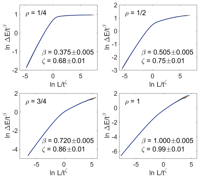
As presented in Fig. 1, the data is very well collapsed according to Eq. (5), although somewhat less so for larger values of $\rho$. In particular we note the excellent collapse at $\rho=1/4$ which according to the RG result of Eq. (3) is the limiting point for which $\beta$ sticks to 1/3. However, we find $\beta=0.375\pm 0.005$, (and $\zeta=0.68\pm 0.01$) in contradiction to RG, but consistent with previous results in Ref. pyhh95 of $\beta=0.364\pm 0.005$ and $\zeta=0.692\pm 0.005$. Indeed, as depicted in Fig. 2, the exponent $\beta$ appears to vary continuously with $\rho$, in contradiction to Eq. (3). As in Ref. pyhh95 , we extend the simulations to $\rho\leq 0$, and throughout this regime obtain $\beta=1/3$ consistent with uncorrelated noise. (We also find $\zeta=2/3$ in this regime through data collapse as in Fig. 1). For larger values of $\rho$, the agreement with RG improves, and the expected random field Ising exponents of $\beta=\zeta=1$ are recovered for $\rho=1$. The continuous variation of $\beta$ for $\rho\leq 1/2$ is similar to observations in previous simulations of DRPM, RSOS, and BD models alf91 ; phss91 ; wb95 ; pyhh95 . We note that the RG exponents are constrained to be exact for uncorrelated noise due to a fluctuation-dissipation condition. The exponents in Eq. (3), however, follow from a non-renormalization of correlated noise amplitude, which in view of the numerics is perhaps questionable.

Figure 2: (a) Variation of $\beta$ with the exponent $\rho$ of spatially correlated energies. There is a small, but clear deviation from the predicted RG exponents (dashed line). (b) Validity of the exponent identities predicted by Galilean invariance; the discrepancies are likely a measure of systematic errors.

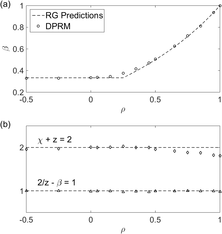
In principle, the scaling relation, Eq. (5), involves two exponents ($\beta$ and $\zeta$, or $\chi$ and $z$). We estimated the roughening exponent $\chi$ from the slope of the collapsed curve in the regime $t\gg L^{z}$. A hallmark of the KPZ equation (even with correlated noise) is Galilean invariance fns77 ; kpz86 , which implies the exponent identity $\chi+z=2$. The explicit check of this identity presented in Fig. 2 appears to indicate its breakdown for $\rho>1/2$. However, simply dividing this identity by $z$, and noting $\beta=\chi/z$, yields a second form $2/z-\beta=1$, which is excellently obeyed by the data! The discrepancy between these two identities is an indication of the systematic errors afflicting the fits, such as the small but systematic curvature in the initial rise of the collapsed curves in Fig. 1, whose slope is used to obtain the exponent $\chi$.

The end-point energy probability distributions are obtained from time $t=10^{3}$ to $t=10^{4}$, in increments of $\Delta t=10^{3}$, and are normalized to have mean 0 and variance 1. The full distributions presented in Fig. 3 are qualitatively similar to the TW-GOE form for $\rho\leq 0$, but shift smoothly towards Gaussian as $\rho$ increases to $\rho=1/2$. Beyond $\rho=1/2$, it is unclear whether the distribution remains Gaussian.

Figure 3: Probability distributions for the optimal energy of DPRM for different correlation exponents $\rho$. The data corresponds to system size $L=10^{6}$ at time $t=5\times 10^{3}$, rescaled to have mean 0 and variance 1. Results are consistent with the TW-GOE form (solid line) for $\rho\leq 0$, and shift smoothly towards Gaussian (dashed line) at $\rho=1/2$.

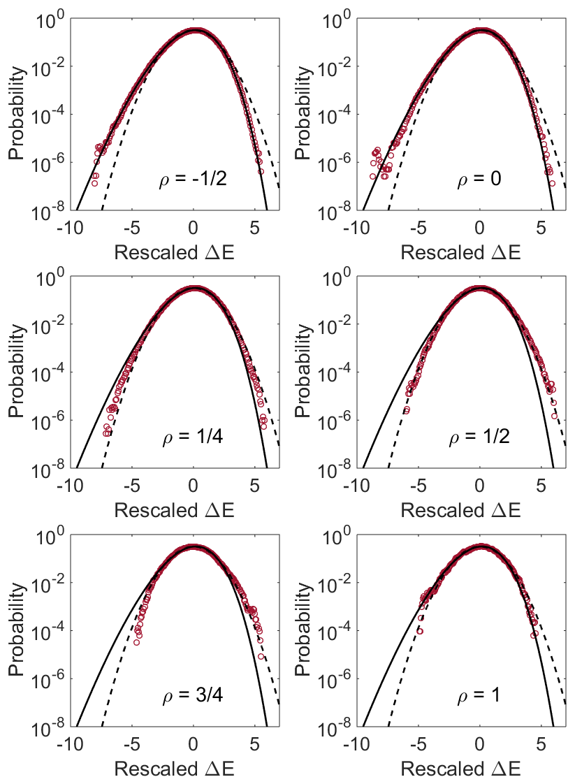
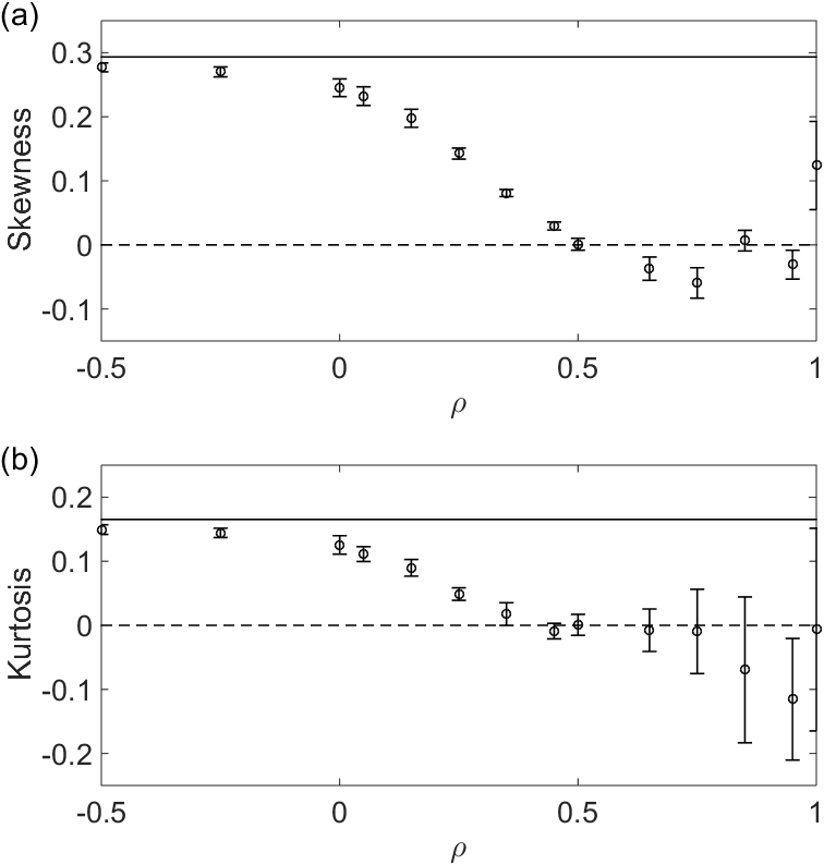
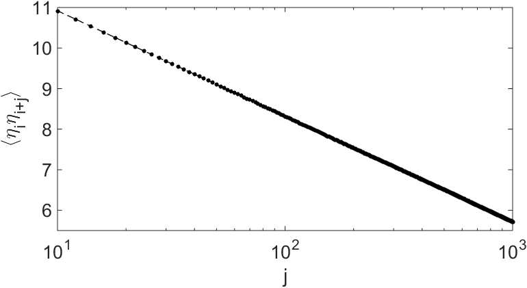
The skewness $s$ and kurtosis $k$, plotted in Fig. 4, are obtained by averaging results over the above snapshots in $t$. In the uncorrelated case, it is possible to estimate the true asymptotic values of $s$ and $k$ using methods developed in Ref. km90 . In the correlated case, however, we run into problems as the uncertainties grow rapidly with correlation. For $\rho\leq 0$, the skewness and kurtosis approach those of the TW-GOE, the limiting distribution for uncorrelated noise. As $\rho$ increases towards 1/2, both $s$ and $k$ decrease to 0, and the distribution becomes more symmetric. In particular, the data suggests that $s,k\rightarrow 0$ as $\rho\rightarrow 1/2$, consistent with a Gaussian distribution. This would be expected if $\rho=1/2$ corresponded to random energies fully correlated in the $x$-direction, but randomly changing along the $t$-direction. The energy of the DPRM would then be a sum of random variables, thus $\beta=1/2$, while the path executes a random walk with $z=2$. The latter is not correct, as the Galilean exponent identity at $\beta=1/2$ leads to the numerically observed exponent of $z=4/3$. We note also that the Fourier transform procedure for generating spatially correlated noise, devised in Ref. mhss96 and used here, actually produces correlations which vary logarithmically at $\rho=1/2$, as $\langle\eta(x,t)\eta(x^{\prime},t^{\prime})\rangle\sim(a-b\ln|x-x^{\prime}|)\delta(t-t^{\prime})$ (see Appendix). Interestingly the RG result (also based on Fourier transformed noise) also predicts the observed $\beta=1/2$. Finally, for $\rho>1/2$, the uncertainty in $s$ and $k$ grow rapidly due to the increased correlations in random energies, and we cannot conclusively state whether the distribution is Gaussian or not. It is of interest to note that another class of distributions, interpolating between TW-GUE and Gaussian, was found in Ref. j07 in the context of random matrix theory, and the convergence of TW distributions to the Gumbel distribution was studied in Ref. ad14 .

Figure 4: (a) Skewness and (b) kurtosis for DPRM with spatially correlated noise, compared to the TW-GOE values (solid lines), $s=0.293$ and $k=0.165$, respectively: Both approach the TW-GOE values for $\rho\leq 0$, and decrease to 0 as $\rho$ increases to 1/2. Beyond $\rho=1/2$, the uncertainties are too large to rule out $s=k=0$.

In summary, we have performed extensive simulations of the DPRM over a spatially correlated landscape. The energy fluctuations are well described by scaling exponents $\beta$ and $z$, extracted by standard data collapse. We find that the exponent identity $2/z-\beta=1$ reflecting Galilean invariance holds for all $\rho$, while the related identity $\chi+z=2$ is apparently violated for $\rho\geq 1/2$, most likely due to systematic errors. While the growth exponent $\beta(\rho)$ is qualitatively similar to predictions of the RG, there are significant deviations for $\rho<1/2$. In particular, for the important value of $\rho=1/2$, at the borderline of correlations growing or decaying with separation, there is strong evidence that $\beta=1/2$, with Gaussian energy fluctuations.

For an uncorrelated landscape, the optimal energy of DPRM behaves as $E=f_{\infty}t+(\Gamma t)^{1/3}\xi$, where $f_{\infty}$ and $\Gamma$ are non-universal, system-dependent parameters, and $\xi$ is a $\mathcal{O}(1)$ random variable obeying TW-GOE statistics. There is currently no analytical prediction for the limiting distribution in the case of correlated noise. From the overall scaling, we can propose an analogous form, $E=f_{\infty}t+(\Gamma t)^{\beta(\rho)}\xi(\rho)$, where $\beta(\rho)$ is the modified growth exponent. The random variable $\xi(\rho)$ is distributed according to TW-GOE statistics for $\rho\leq 0$. A priori one could have imagined that the distribution retains the TW form in general, or that it discontinuously transitions to a different distribution for $\rho>0$. Instead, we observe a smooth shift as $\rho$ increases, to a Gaussian form at $\rho=1/2$. For $\rho>1/2$, the uncertainty in skewness and kurtosis become too significant to conclude whether the distribution is Gaussian. We thus find a class of distributions, interpolating between TW and Gaussian, which governs the statistics of DPRM with spatially correlated noise.

We are grateful to T. Halpin-Healy, A. Rosso, and G. Bunin for illuminating discussions, and financial support from the NSF through grant No. DMR-12-06323. This work was partly completed at KITP, which is supported in part by the NSF under grant PHY05-51164. SC was also supported by MIT through the Thomas Frank Fellowship.

Appendix: Algorithm for generating correlated noise

We present here the method used for generating correlated noise developed in Ref. mhss96 . Note that a similar method was developed in Ref. pyhh95 to study DPRM and BD models with correlated noise.

Figure A1: Log-log plot of correlation of generated noise with $\rho<1/2$ for system size $L=10^{6}$. The data for $\rho=0.35$, $\rho=0.25$, and $\rho=0.15$ are plotted (from top to bottom). The best fit lines (dashed) give $\rho=0.33\pm 0.02$, $\rho=0.24\pm 0.02$, and $\rho=0.15\pm 0.01$ respectively.

Figure A2: Log-log plot of correlation of generated noise with $\rho>1/2$ for system size $L=10^{6}$. The data for $\rho=0.85$, $\rho=0.75$, and $\rho=0.65$ are plotted (from top to bottom). The best fit lines (dashed) give $\rho=0.86\pm 0.03$, $\rho=0.77\pm 0.04$, and $\rho=0.69\pm 0.04$ respectively.

Figure A3: Semilog plot of correlation of generated noise with $\rho=1/2$ for system size $L=10^{6}$. The correlation decays logarithmically with separation, and the best fit line (dashed) gives $C(j)=-1.13\ln|j|+13.52$.

In $d=1$ dimension, the goal is to use a sequence of Gaussian i.i.d. random variables $\{u_{i}\}_{i=1,\ldots,L}$ to generate a sequence $\{\eta_{i}\}_{i=1,\ldots,L}$ with correlation function mhkz89

$$C(j)=\langle\eta_{i}\eta_{i+j}\rangle\sim j^{2\rho-1},\;\;\;\;\;\;\;\;j\rightarrow\infty.$$ (A1)

Taking the Fourier transform gives the spectral density function $S(q)$, which has asmptotic form

$$S(q)=\langle\eta_{q}\eta_{-q}\rangle\sim q^{-2\rho},\;\;\;\;\;\;\;\;q\rightarrow 0.$$ (A2)

The correlated random variables can then be obtained from the relation

$$\eta_{q}=[S(q)]^{1/2}u_{q},$$ (A3)

where $\{\eta_{q}\}$ and $\{u_{q}\}$ are the Fourier transform coefficients of $\{\eta_{i}\}$ and $\{u_{i}\}$, respectively.

As in Ref. mhss96 , we define the correlation function to be

$$C(j)\equiv(1+j^{2})^{\rho-1/2},$$ (A4)

on the interval $j\in[-L/2,L/2]$. This then has the same asymptotic power law decay as in Eq. (A1). The spectral density can be calculated analytically as the discrete Fourier transform,

$$S(q)=\frac{2\pi^{1/2}}{\Gamma(-\rho+1)}\left(\frac{q}{2}\right)^{-\rho}K_{\rho}(q),$$ (A5)

where $q=2\pi n/L$ with $n=-L/2,\ldots,L/2$, and $K_{\rho}$ is the modified Bessel function of the second kind of order $\rho$. We define $S(q=0)=0$ to avoid any divergences. For $\rho>0$, the modified Bessel function has asymptotic form

$$K_{\rho}(q)\sim\left\{\begin{array}[]{ll}\displaystyle\frac{\Gamma(\rho)}{2}\left(\frac{2}{q}\right)^{\rho},&q\ll 1,\\ \displaystyle\sqrt{\frac{\pi}{2q}}e^{-q},&q\gg 1.\end{array}\right.$$ (A6)

As $q\rightarrow 0$, we recover the asymtotic form in Eq. (A2).

The process for generating the correlated noise used to study DPRM can then be summarized in the following steps.

1. Generate Gaussian i.i.d. random variables $\{u_{i}\}$, and calculate $\{u_{q}\}$ using the fast Fourier transform.

2. Calculate the spectral density function $S(q)$ using Eq. (A5), (A6).

3. Calculate $\{\eta_{q}\}$ using Eq. (A3), and calculate $\{\eta_{i}\}$ using the inverse Fourier transform.

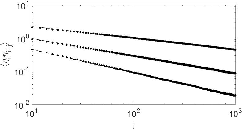
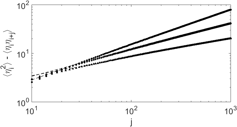
For the DPRM model we simulated, the system size is $L=10^{6}$, evolved over $t=10^{4}$ time steps. We check the correlation of the noise generated using the above method by averaging over $10^{2}$ realizations. The results for $\rho<1/2$ and $\rho>1/2$ are plotted in Fig. A1 and A2, respectively, and we see that the data is in good agreement with the expected values of $\rho$ up to a separation of $j=10^{3}$. In the special case $\rho=1/2$, we find that the correlation decays logarithmically with separation, as shown in Fig. A3.

References

- (1)
- (2) C. A. Tracy and H. Widom, Commun. Math. Phys. 177, 727 (1996).
- (3) N. Wolchover, Quanta Magazine, 10/27 (2014).
- (4) S. N. Majumdar and S. Nechaev, Phys. Rev. E 72, 020901 (R) (2005).
- (5) Ch. Hajiyev, ISA Transactions, 51, 189 (2012).
- (6) M. Kardar and Y.-C. Zhang, Phys. Rev. Lett. 58, 2087 (1987).
- (7) T. Halpin-Healy and Y.-C. Zhang, Phys. Rep. 254, 215 (1995).
- (8) T. Halpin-Healy and K. A. Takeuchi, J. Stat. Phys. 160, 794 (2015).
- (9) I. Corwin, Random Matrices: Theory Appl. 1, 1130001 (2012).
- (10) J. Quastel and H. Spohn, J. Stat. Phys. 160, 965 (2015).
- (11) E. Medina, T. Hwa, M. Kardar, and Y.-C. Zhang, Phys. Rev. A 39, 3053 (1989).
- (12) M. Kardar, G. Parisi, and Y.-C. Zhang, Phys. Rev. Lett. 56, 889 (1986).
- (13) J. M. Kim, M. A. Moore, and A. J. Bray, Phys. Rev. A 44, 2345 (1991).
- (14) J. M. Kim, M. A. Moore, and A. J. Bray, Phys. Rev. A 44, R4782 (1991).
- (15) T. Halpin-Healy, Phys. Rev. A 44, R3415 (1991).
- (16) T. Halpin-Healy, Phys. Rev. Lett. 109 170602 (2012); Phys. Rev. E 88, 042118 (2013).
- (17) T. Halpin-Healy and Y. Lin, Phys. Rev. E 89, 010103(R) (2014).
- (18) T. Gueudre, P. Le Doussal, J.-P. Bouchaud, and A. Rosso, Phys. Rev. E 91 062110 (2015).
- (19) M. Eden, Proc. 4th Berkeley Symp. on Mathematical Statistics and Probability (University of California Press 1961).
- (20) P. Meakin, J. Phys. A: Math. Gen. 20, L1113 (1987).
- (21) S. Roux, A. Hansen, and E. L. Hinrichsen, J. Phys. A: Math. Gen. 24 L295 (1991).
- (22) J. M. Kim and J. M. Kosterlitz, Phys. Rev. Lett. 62, 2289 (1989).
- (23) J. M. Kim, J. M. Kosterlitz, and T. Ala-Nissila, J. Phys. A: Math. Gen. 24 5569 (1991).
- (24) M. J. Vold, J. Colloid Sci. 14, 168 (1959).
- (25) M. Kardar, Nucl. Phys. B290 [FS20], 582 (1987).
- (26) T. Sasamoto, and H. Spohn, Phys. Rev. Lett. 104, 230602 (2010).
- (27) K. Johansson, Commun. Math. Phys. 209, 437 (2000).
- (28) M. Prähofer and H. Spohn, Phys. Rev. Lett. 84, 4882 (2000).
- (29) Y.-C. Zhang, Physics A: Statistical Mechanics and its Applications, 170, 1 (1990).
- (30) J. Krug, J. de Phys. I, 1, 9 (1991).
- (31) G. Biroli, J.-P. Bouchaud, and M. Potters, J. Stat. Mech.: Theory and Experiment, 2007, P07019 (2007).
- (32) D. Forster, D. R. Nelson, and M. J. Stephen, Phys. Rev. A 16, 732 (1977).
- (33) E. Frey, U. C. Täuber, and H. K. Janssen, Europhys. Lett. 47, 14 (1999).
- (34) T. Kloss, L. Canet, B. Delamotte, and N. Wschebor, Phys. Rev. E 89, 022108 (2014).
- (35) H. A. Makse, S. Havlin, M. Schwartz, H. E. Stanley, Phys. Rev. E 53, 5445 (1996).
- (36) N.-N. Pang, Y.-K. Yu, and T. Halpin-Healy, Phys. Rev. E 52, 3224 (1995).
- (37) J. G. Amar, P.-M. Lam, and F. Family, Phys. Rev. A 43, 4548 (1991).
- (38) C.-K. Peng, S. Havlin, M. Schwartz, and H. E. Stanley, Phys. Rev. A 44, R2239 (1991).
- (39) M. Wu and K. Y. R. Billah, Phys. Rev. E 51, 995 (1995).
- (40) J. Krug and P. Meakin, J. Phys. A: Math. Gen. 23, L987 (1990).
- (41) K. Johansson, Probab. Theory Related Fields 138, 75 (2007).
- (42) R. Allez and L. Dumaz, J. Stat. Phys. 156, 1146 (2014).