Abstract

We identify 339 known and 316 new variable stars of various types among 250000 lightcurves obtained by digitizing 167 $30\times 30$ cm photographic plates of the Moscow collection. We use these data to conduct a comprehensive test of 18 statistical characteristics (variability indices) in search for the best general-purpose variability detection statistic. We find that the highest peak on the DFT periodogram, interquartile range, median absolute deviation, and Stetson’s $L$ index are the most efficient in recovering variable objects from the set of photographic lightcurves used in our test.

Keywords: variable stars, photographic photometry

1 Introduction

The simplest way to find a variable object is to compare its brightness on two images of the sky taken at different times. However, this works well only if the amplitude of brightness variations over that time is large compared to measurement errors associated with the images. If we have a lightcurve that includes measurements of an object’s brightness at multiple times, in principle, we may “average out” individual measurement errors and recover a small-amplitude variability. Two problems complicate this in practice: poor knowledge of measurement errors (which is especially true for photographic data) and a priori unknown pattern of object’s variations. One may overcome the first problem by assuming that objects that are close to each other in the sky and have similar brightness are measured with about the same accuracy on a given set of images. To overcome the second problem one needs a variability indicator that responds to a wide variety of brightness variation patterns.

In this work we compare 18 statistical characteristics (Table 1) that quantify “how variable” an object is. The indices belong to three classes: i) scatter-based indices quantifying the scatter of brightness measurements in a lightcurve; ii) correlation-based indices characterize the degree of correlation between the consecutive brightness measurements; ii) period-search methods look for periodic brightness variations.

The last column of Table 1 refers to the publications in which one may find the definitions of these indices, so here we mention only the more unconventional ones. The interquartile range, IQR [e.g. 1] is a robust measure of scatter. It includes the inner 50% of measurement values (i.e. excludes 25% of the brightest and 25% of the faintest flux measurements). Unlike the commonly used root mean square, the IQR is insensitive to outliers. To use [2] and [3] period search techniques as “variability indices” we compute the periodogram in the 0.1–10 d with steps in frequency corresponding to a phase shift of 0.01 between the first and the last points in a lightcurve. The value of the highest peak on the periodogram is then used as a variability index.

2 Comparison technique and results

To test the performance of the variability indices we use 167 $30\times 30$ cm photographic plates ($10^{\circ}\times 10^{\circ}$ field of view with a limiting magnitude of $\sim 17.5$ pg) of the 104 Her field. The plates are obtained with a 40 cm $F=160$ cm astrograph in 1976-1994, digitized with a flatbed scanner and split into 173 $52^{\prime}\times 52^{\prime}$ partly overlapping subfields that were independently processed with the VaST software. The lightcurves of 250000 stars were extracted and searched for variability using the technique discussed by [4, 5, 6, 7]. The dataset includes 339 known and 316 new variable stars, among them 341 eclipsing binaries, 165 RR Lyrae stars and 139 red periodic, semi-periodic and irregular variables. Having constructed the comprehensive list of true variable stars, we investigate how well these variables can be extracted from the dataset using various variability indices.

To quantify the quality of candidate variables selection provided by each variability index following [8, 9, 10], we compute the completeness $C$ and purity $P$:

$$C=\frac{\mathrm{Number\,\,of\,\,selected\,\,variables}}{\mathrm{Total\,\,number\,\,of\,\,confirmed\,\,variables}}$$ (1)

$$P=\frac{\mathrm{Number\,\,of\,\,selected\,\,variables}}{\mathrm{Total\,\,number\,\,of\,\,selected\,\,candidates}}$$ (2)

as well as the fidelity $F_{1}$-score which is the harmonic mean of the two parameters:

$$F_{1}=2(C\times P)/(C+P).$$ (3)

$F_{1}=1$ for a perfect selection when all true variables and no false candidates pass the selection criteria while $F_{1}=0$ if no true variables are selected.

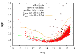
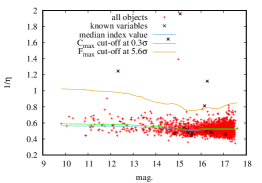
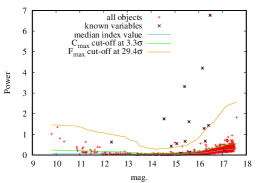
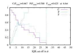
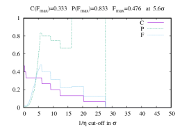
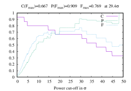
For each variability index we estimate its expected value and its scatter, $\sigma$, as a function of magnitude (Fig. 1). Candidate variables are then selected as objects having their variability index value $>n\sigma$ above the expected value of this index for the object’s magnitude. The selection is repeated for $n$ in the range 0–50. The resulting $C$, $P$, and $F_{1}$ values as a function of $n$ are presented in Fig. 2. The selection resulting in the highest $F_{1}$-score is used to compare the indices. This way the optimal cut-off value $n\sigma$ is used for each index. The distribution of the expected index values for a given magnitude is non-Gaussian, therefore a simple choice like a $3\sigma$ cut-off might not be the optimal one for some indices.

The results of variability indices comparison are presented in Table 1. The table presents the information taken into account by each index (in addition to the measured magnitudes themselves) that may include estimated photometric errorbars, order of points in a lightcurve and exact times of observations. It presents the maximum $F_{1}$-score reached by a selection using each index. We consider the index with the highest value of $F_{1~{}\rm max}$ as the most efficient in selecting true variable stars. Since $F_{1}$ characterizes only the selected candidates, but does not take into account the rejected, presumably non-variable, objects, Table 1 also lists a fraction of objects that do not pass the selection (at the cut-off value corresponding to $F_{1~{}\rm max}$), $R_{F_{1~{}\rm max}}$, as an auxiliary measure of variability index performance. Finally, Table 1 reports the maximum completeness, $C_{\rm max}$, reached by each index at a selection cut-off of $n\sigma$ where $n\geq 0$. The values of $C_{\rm max}<1$ indicate that the index cannot recover some variable stars, even at a low selection threshold (corresponding to a large number of false candidates). All $F_{1~{}\rm max}$, $R_{F_{1~{}\rm max}}$, and $C_{\rm max}$ values presented in Table 1 are the median values computed over the 173 subfields.

3 Conclusions

Table 1 indicates that the highest peak on the DFT periodogram, ${\rm IQR}$, ${\rm MAD}$, and Stetson’s $L$ index are the most efficient in recovering variable objects from the set of photographic lightcurves used for the test. These indices can be recommended for the future searches of variable objects using photographic lightcurves. Some correlation-based indices (like the $I$ index) are only able to recover objects varying on timescales longer than the typical lightcurve sampling time and, therefore, are not good general-purpose variability indicators for (typically) sparsely sampled photographic lightcurves. Constant stars with corrupted measurements (e.g. due to blending with a nearby star) may pass the selection threshold even for the best identified variability indices. The need to reject such badly measured stars through a visual inspection of lightcurves and images so far prevents a full automation of variability searches.

Figure 1: Variability indices IQR, $1/\eta$, and the highest DFT peak plotted as a function of magnitude for one of the $52^{\prime}\times 52^{\prime}$ subfields. Variable stars are marked with ’x’. The curves represent the expected values of the indices for a given magnitude and selection thresholds corresponding to the best trade-off between the completeness and purity of the candidates list ($F_{\rm max}$) and the maximum completeness of the list ($C_{\rm max}$).

Figure 2: Variable star selection completeness ($C$, Eq. 1), purity ($P$, Eq. 2), and $F_{1}$-score (Eq. 3) as a function of selection threshold for the variability indices IQR, $1/\eta$, and the highest DFT peak. The plots are for the dataset presented at Fig. 1.

Table 1: Variability indices

Index	Errors	Order	Time	$F_{1~{}\rm max}$	$R_{F_{1~{}\rm max}}$	$C_{\rm max}$	Ref.
Scatter-based indices
$\chi_{\rm red}^{2}$	$\checkmark$			0.111	0.979	1.000	[11]
$\sigma$				0.182	0.987	1.000	[7]
${\rm MAD}$				0.400	0.995	1.000	[12]
${\rm IQR}$				0.400	0.995	1.000	this work
${\rm RoMS}$	$\checkmark$			0.333	0.994	1.000	[13]
$\sigma_{\rm NXS}^{2}$	$\checkmark$			0.200	0.990	1.000	[14]
$v$	$\checkmark$			0.039	0.932	1.000	[15]
Correlation-based indices
$l_{1}$		$\checkmark$		0.250	0.997	0.667	[16]
$I$	$\checkmark$	$\checkmark$	$\checkmark$	0.154	0.989	0.667	[17]
$J$	$\checkmark$	$\checkmark$	$\checkmark$	0.250	0.994	1.000	[18]
$J({\rm time})$	$\checkmark$	$\checkmark$	$\checkmark$	0.250	0.995	0.750	[19]
$L$	$\checkmark$	$\checkmark$	$\checkmark$	0.400	0.996	1.000	[18]
$E_{x}$	$\checkmark$	$\checkmark$	$\checkmark$	0.222	0.993	1.000	[20]
$1/\eta$		$\checkmark$		0.250	0.998	0.667	[21]
$\mathcal{E}_{\mathcal{A}}$		$\checkmark$	$\checkmark$	0.014	0.860	0.600	[22]
$S_{B}$	$\checkmark$	$\checkmark$		0.143	0.987	1.000	[23]
Period search
${\rm L-K}$		$\checkmark$	$\checkmark$	0.087	0.981	1.000	[2]
${\rm DFT}$		$\checkmark$	$\checkmark$	0.500	0.995	1.000	[3]

Acknowledgements. KVS is supported by the European Space Agency (ESA) under the “Hubble Catalog of Variables” program, contract No. 4000112940. This work is supported by the grant from the Program “Transition and explosive processes in the Universe” of the Presidium of Russian Academy of Sciences and the RFBR grant 13-02-00664.

References

- [1] D.-W. Kim, et al., A&A 566, A43 (2014).
- [2] J. Lafler, T. D. Kinman, ApJS 11, 216 (1965).
- [3] T. J. Deeming, Ap&SS 36, 137 (1975).
- [4] K. Sokolovsky, et al., Astroplate 2014 (2014), p. 79.
- [5] K. V. Sokolovsky, et al., Astronomy Reports 58, 319 (2014).
- [6] D. M. Kolesnikova, et al., Astronomy Reports 54, 1000 (2010).
- [7] D. M. Kolesnikova, L. A. Sat, K. V. Sokolovsky, S. V. Antipin, N. N. Samus, Acta Astron. 58, 279 (2008).
- [8] D.-W. Kim, et al., ApJ 735, 68 (2011).
- [9] M. J. Graham, et al., MNRAS 439, 703 (2014).
- [10] D.-W. Kim, C. A. L. Bailer-Jones, A&A 587, A18 (2016).
- [11] J. A. de Diego, AJ 139, 1269 (2010).
- [12] M. Zhang, et al., PASP 128, 035001 (2016).
- [13] M. B. Rose, E. G. Hintz, AJ 134, 2067 (2007).
- [14] K. Nandra, I. M. George, R. F. Mushotzky, T. J. Turner, T. Yaqoob, ApJ 476, 70 (1997).
- [15] K. V. Sokolovsky, Y. Y. Kovalev, Y. A. Kovalev, N. A. Nizhelskiy, G. V. Zhekanis, Astronomische Nachrichten 330, 199 (2009).
- [16] D.-W. Kim, P. Protopapas, C. Alcock, Y.-I. Byun, R. Khardon, Astronomical Data Analysis Software and Systems XX, I. N. Evans, A. Accomazzi, D. J. Mink, A. H. Rots, eds. (2011), vol. 442 of Astronomical Society of the Pacific Conference Series, p. 447.
- [17] D. L. Welch, P. B. Stetson, AJ 105, 1813 (1993).
- [18] P. B. Stetson, PASP 108, 851 (1996).
- [19] T. Fruth, et al., AJ 143, 140 (2012).
- [20] J. R. Parks, P. Plavchan, R. J. White, A. H. Gee, ApJS 211, 3 (2014).
- [21] M.-S. Shin, M. Sekora, Y.-I. Byun, MNRAS 400, 1897 (2009).
- [22] N. Mowlavi, A&A 568, A78 (2014).
- [23] R. Figuera Jaimes, A. Arellano Ferro, D. M. Bramich, S. Giridhar, K. Kuppuswamy, A&A 556, A20 (2013).