A Comparison and Joint Analysis of Sunyaev-Zel’dovich Effect Measurements from Planck and Bolocam for a set of 47 Massive Galaxy Clusters

Abstract

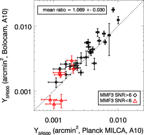
We measure the SZ signal toward a set of 47 clusters with a median mass of $9.5\times 10^{14}$ M_☉ and a median redshift of 0.40 using data from Planck and the ground-based Bolocam receiver. When Planck XMM-like masses are used to set the scale radius $\theta_{\textrm{s}}$, we find consistency between the integrated SZ signal, $Y_{\textrm{5R500}}$, derived from Bolocam and Planck based on gNFW model fits using A10 shape parameters, with an average ratio of $1.069\pm 0.030$ (allowing for the $\simeq 5$% Bolocam flux calibration uncertainty). We also perform a joint fit to the Bolocam and Planck data using a modified A10 model with the outer logarithmic slope $\beta$ allowed to vary, finding $\beta=6.13\pm 0.16\pm 0.76$ (measurement error followed by intrinsic scatter). In addition, we find that the value of $\beta$ scales with mass and redshift according to $\beta\propto M^{0.077\pm 0.026}\times(1+z)^{-0.06\pm 0.09}$. This mass scaling is in good agreement with recent simulations. We do not observe the strong trend of $\beta$ with redshift seen in simulations, though we conclude that this is most likely due to our sample selection. Finally, we use Bolocam measurements of $Y_{500}$ to test the accuracy of the Planck completeness estimate. We find consistency, with the actual number of Planck detections falling approximately $1\sigma$ below the expectation from Bolocam. We translate this small difference into a constraint on the the effective mass bias for the Planck cluster cosmology results, with $(1-b)=0.93\pm 0.06$.

1. Introduction

The Sunyaev-Zel’dovich (SZ) effect has emerged as a valuable observational tool for studying galaxy clusters, particularly with the dramatic improvements in instrumentation that have occurred over the past decade. For example, the South Pole Telescope (SPT, Bleem et al., 2015), the Atacama Cosmology Telescope (ACT, Hasselfield et al., 2013), and Planck (Planck Collaboration et al., 2015d) have delivered catalogs with a combined total of more than 1000 SZ-detected clusters. Beyond these large surveys, detailed studies of the gaseous intra-cluster medium (ICM) have been enabled by an additional set of pointed SZ facilities with broad spectral coverage and/or excellent angular resolution such as the Multiplexed SQUID/TES Array at Ninety GHz (MUSTANG, Mason et al., 2010) the New IRAM KID Arrays (NIKA, Adam et al., 2016), and the Multiwavelength Submillimeter Inductance Camera (MUSIC, Sayers et al., 2016).

As the range of SZ instrumentation has become more diverse, the benefits of joint analyses using multiple datasets have increased. For example, a wide range of studies have used data from two or more SZ receivers in order to measure the spectral shape of the SZ signal (e.g., Kitayama et al., 2004; Zemcov et al., 2010; Mauskopf et al., 2012), mainly for the purpose of constraining the ICM velocity via the kinetic SZ signal, but also to characterize relativistic corrections to the classical SZ spectrum (e.g., Sunyaev & Zeldovich, 1980; Nozawa et al., 1998; Chluba et al., 2012). Furthermore, recent analyses have begun to exploit the different angular sensitivities of the SZ facilities in order to obtain a more complete spatial picture of the cluster (e.g., Romero et al., 2015; Young et al., 2015; Rodríguez-Gonzálvez et al., 2015).

In order for these joint analyses to be useful, the various SZ instruments must provide measurements of the SZ signal that are consistent. Historically, this was often not the case, likely due to large systematic errors in the measurements (e.g., see the detailed discussion in Birkinshaw, 1999). However, the situation has improved considerably with advances in modern SZ instrumentation, and good agreement has been seen in most recent comparisons (e.g., Reese et al., 2012; Mauskopf et al., 2012; Rodríguez-Gonzálvez et al., 2015; Sayers et al., 2016). Modest inconsistencies do still appear, although they are often the result of assuming different spatial templates when performing the SZ analyses for separate instruments (e.g., Benson et al., 2004; Planck Collaboration et al., 2013a; Perrott et al., 2015). In sum, the systematics that plagued early SZ measurements appear to be largely absent from modern data. This fact, combined with the high degree of complementarity between different SZ facilities, has opened a promising future for detailed cluster studies using multiple SZ datasets.

In this work, we use SZ measurements from Planck and the ground-based receiver Bolocam to study a set of 47 massive clusters. The manuscript is organized as follows. In Section 2, the parametric model used to describe the data is introduced, and in Section 3 the SZ data from Planck and Bolocam are detailed. Section 4 compares the SZ signals measured by Planck and Bolocam, and Section 5 presents the results from joint fits to the two datasets. In Section 6, we use Bolocam SZ measurements to perform a test of the Planck cluster survey completeness, and a summary of the manuscript is given in Section 7.

2. The SZ Effect

The thermal SZ effect (Sunyaev & Zel’dovich, 1972) describes the Compton scattering of CMB photons with hot electrons in the ICM according to

$$\Delta T(\nu) = f(\nu,T_{\mathrm{e}})y$$

$$y = \int\frac{k_{\textrm{B}}\sigma_{\textrm{T}}}{m_{\mathrm{e}}c^{2}}p_{\mathrm{e}}dl$$

where $\Delta T(\nu)$ is the observed surface brightness fluctuation in units of CMB temperature at the frequency $\nu$, $T_{\textrm{e}}$ is the ICM electron temperature, $f(\nu,T_{\textrm{e}})$ describes the spectral dependence of the SZ signal including relativistic corrections (e.g., Rephaeli, 1995; Itoh et al., 1998; Nozawa et al., 1998; Itoh & Nozawa, 2004; Chluba et al., 2012), $y$ is the SZ Compton parameter, $k_{\textrm{B}}$ is Boltzmann’s constant, $\sigma_{\textrm{T}}$ is the Thompson cross section, $m_{\textrm{e}}$ is the electron mass, $c$ is the speed of light, $p_{\textrm{e}}$ is the ICM electron pressure, and $dl$ is along the line of sight. In the absence of relativistic corrections, which are generally small and/or constrained using a spectroscopic X-ray measurement of the value of $T_{\textrm{e}}$, the SZ brightness gives a direct measure of the integrated ICM pressure. Therefore, SZ measurements are often used to constrain parametric models of the pressure, such as the generalized Navarro, Frenk, and White (gNFW, Navarro et al. 1997) model described in the following section.

2.1. The gNFW Model

Nagai et al. (2007) proposed the use of a gNFW model to describe cluster pressure profiles according to

$$P(R)=\frac{P_{0}}{(R/R_{\textrm{s}})^{\gamma}(1+(R/R_{\textrm{s}})^{\alpha})^{(\beta-\gamma)/\alpha}}$$

where $P(R)$ is the pressure as a function of radius, $P_{0}$ is the normalization factor, $R_{\textrm{s}}$ is the scale radius, and $\alpha$, $\beta$, and $\gamma$ control the logarithmic slope of the profile at $R\sim R_{\textrm{s}}$, $R\gg R_{\textrm{s}}$, and $R\ll R_{\textrm{s}}$. Often, the radial coordinates are rescaled to angular coordinates denoted by $\theta$ and $\theta_{\textrm{s}}$, and $R_{\textrm{s}}$ is often recast in terms of a concentration parameter, with

$$C_{500}=R_{500}/R_{\textrm{s}}=\theta_{500}/\theta_{\textrm{s}},$$

and $R_{500}$ denoting the radius where the average enclosed density is 500 times the critical density of the universe. Therefore, for a given value of $C_{500}$, the values of $R_{\textrm{s}}$ and $\theta_{\textrm{s}}$ are directly related to the cluster mass, $M_{500}$. Furthermore, the normalization is often given in terms the SZ observable integrated within a specific radius, for example

$$Y_{5\textrm{R}500}=\int^{5\times\theta_{500}}_{0}y\times 2\pi\theta d\theta.$$

Nagai et al. (2007) noted that, when $P_{0}$ is scaled according to a factor that depends on the cluster’s mass and redshift and $R_{\textrm{s}}$ is recast in terms of $C_{500}$, that a single set of values for $\alpha$, $\beta$, and $\gamma$ provide an approximately universal description of any cluster’s pressure profile. Subsequently, several groups have published different values for these logarithmic slopes based on different samples, data, and analysis techniques (e.g., Arnaud et al. 2010; Plagge et al. 2010; Planck Collaboration et al. 2013b; Sayers et al. 2013; McDonald et al. 2014 and Mantz et al. 2016), and the values given by Arnaud et al. (2010) are the most widely used. The corresponding gNFW shape with $C_{500}=1.18$, $\alpha=1.05$, $\beta=5.49$, and $\gamma=0.31$ is often referred to as the A10 model.

3. Data

3.1. Cluster Sample

This study focuses on a set of 47 clusters with publicly available data from Bolocam and Chandra. Data for 45 of these clusters were published in Czakon et al. (2015), who named that sample the Bolocam X-ray SZ (BoXSZ) sample. Throughout this work, the slightly expanded set of 47 clusters is referred to as the BoXSZ⁺ sample (see Table 1). Based on the Planck MMF3 detection algorithm, 32 BoXSZ⁺ clusters were detected by Planck, with 25 detected at a high enough significance to be included in the Planck cluster cosmology analysis (Planck Collaboration et al., 2015c, d).

Table 1Cluster Sample

		RA	dec	$M_{500}$	$\theta_{500}$ (CXO)	$\theta_{500}$ (XMM)	Planck	Bolocam
Cluster	$z$
		hr	deg	$10^{14}$ M⊙	arcmin	arcmin	SNR	SNR
Abell 2204	0.15	16:32:47	$+$05:34:32	$10.3\pm 1.5$	$9.2\pm 0.4$	$8.6\pm 0.2$	16.3	22.3
Abell 1689	0.18	13:11:29	$-$01:20:27	$10.5\pm 1.5$	$7.9\pm 0.4$	$7.6\pm 0.2$	16.7	06.2
Abell 0383	0.19	02:48:03	$-$03:31:46	0$4.7\pm 0.8$	$5.8\pm 0.3$	—	—	09.6
Abell 0209	0.21	01:31:53	$-$13:36:48	$12.6\pm 1.9$	$7.4\pm 0.4$	$6.6\pm 0.2$	17.1	13.9
Abell 0963	0.21	10:17:03	$+$39:02:52	0$6.8\pm 1.0$	$6.0\pm 0.3$	$5.8\pm 0.2$	08.8	08.3
Abell 1423	0.21	11:57:17	$+$33:36:39	0$8.7\pm 2.0$	$6.5\pm 0.5$	$5.7\pm 0.2$	09.7	05.8
Abell 2261	0.22	17:22:26	$+$32:07:58	$14.4\pm 2.6$	$7.4\pm 0.4$	$6.1\pm 0.2$	13.5	10.2
Abell 0267	0.23	01:52:42	$+$01:00:29	0$6.6\pm 1.1$	$5.5\pm 0.3$	$5.0\pm 0.3$	05.4	09.6
Abell 2219	0.23	16:40:20	$+$46:42:29	$18.9\pm 2.5$	$7.9\pm 0.4$	$6.7\pm 0.1$	26.3	11.1
RX J2129.6$+$0005	0.24	21:29:39	$+$00:05:17	0$7.7\pm 1.2$	$5.6\pm 0.3$	$4.6\pm 0.3$	04.8	08.0
Abell 1835	0.25	14:01:01	$+$02:52:40	$12.3\pm 1.4$	$6.3\pm 0.3$	$5.8\pm 0.2$	14.4	15.7
Abell 0697	0.28	08:42:57	$+$36:21:56	$17.1\pm 2.9$	$6.5\pm 0.4$	$5.6\pm 0.1$	18.9	22.6
Abell 0611	0.29	08:00:56	$+$36:03:25	0$7.4\pm 1.1$	$4.7\pm 0.2$	$4.3\pm 0.2$	06.8	10.8
Abell 2744	0.31	00:14:15	$-$30:23:31	$17.6\pm 3.0$	$6.0\pm 0.5$	$4.9\pm 0.1$	14.1	15.9
MACS J2140.2$-$2339	0.31	21:40:15	$-$23:39:40	0$4.7\pm 0.6$	$3.9\pm 0.1$	—	—	06.5
Abell S1063	0.35	22:48:44	$-$44:31:45	$22.2\pm 3.4$	$5.9\pm 0.3$	$4.8\pm 0.1$	20.7	13.6
MACS J1931.8$-$2635	0.35	19:31:49	$-$26:34:33	0$9.9\pm 1.6$	$4.5\pm 0.2$	$3.9\pm 0.2$	06.1	10.1
MACS J1115.8$+$0129	0.36	11:15:51	$+$01:29:54	0$8.6\pm 1.2$	$4.2\pm 0.2$	$3.8\pm 0.2$	07.1	10.9
MACS J1532.8$+$3021	0.36	15:32:53	$+$30:20:58	0$9.5\pm 1.7$	$4.3\pm 0.3$	—	—	08.0
Abell 0370	0.38	02:39:53	$-$01:34:38	$11.7\pm 2.1$	$4.5\pm 0.3$	$3.9\pm 0.1$	07.6	12.8
MACS J1720.2$+$3536	0.39	17:20:16	$+$35:36:22	0$6.3\pm 1.1$	$3.6\pm 0.2$	$3.6\pm 0.2$	06.5	10.6
MACS J0429.6$-$0253	0.40	04:29:36	$-$02:53:05	0$5.8\pm 0.8$	$3.4\pm 0.2$	—	—	08.9
MACS J2211.7$-$0349	0.40	22:11:45	$-$03:49:42	$18.1\pm 2.5$	$5.0\pm 0.2$	$4.1\pm 0.1$	11.8	14.7
ZwCl 0024.0$+$1652	0.40	00:26:35	$+$17:09:40	0$4.4\pm 1.6$	$3.1\pm 0.3$	—	—	03.3
MACS J0416.1$-$2403	0.42	04:16:08	$-$24:04:13	0$9.1\pm 2.0$	$3.8\pm 0.5$	$1.5\pm 0.2$	04.7	08.5
MACS J0451.9$+$0006	0.43	04:51:54	$+$00:06:18	0$6.3\pm 1.1$	$3.3\pm 0.2$	—	—	08.1
MACS J0417.5$-$1154	0.44	04:17:34	$-$11:54:27	$22.1\pm 2.7$	$4.9\pm 0.2$	$4.0\pm 0.1$	13.3	22.7
MACS J1206.2$-$0847	0.44	12:06:12	$-$08:48:05	$19.2\pm 3.0$	$4.7\pm 0.2$	$3.9\pm 0.1$	13.3	21.7
MACS J0329.6$-$0211	0.45	03:29:41	$-$02:11:46	0$7.9\pm 1.3$	$3.4\pm 0.2$	—	—	12.1
MACS J1347.5$-$1144	0.45	13:47:30	$-$11:45:08	$21.7\pm 3.0$	$4.8\pm 0.2$	$3.8\pm 0.1$	11.2	36.6
MACS J1311.0$-$0311	0.49	13:11:01	$-$03:10:39	0$3.9\pm 0.5$	$2.6\pm 0.1$	—	—	09.6
MACS J2214.9$-$1400	0.50	22:14:57	$-$14:00:11	$13.2\pm 2.3$	$3.8\pm 0.2$	$3.3\pm 0.1$	08.3	12.6
MACS J0257.1$-$2325	0.51	02:57:09	$-$23:26:03	0$8.5\pm 1.3$	$3.2\pm 0.2$	$2.9\pm 0.1$	05.4	10.1
MACS J0911.2$+$1746	0.51	09:11:10	$+$17:46:31	0$9.0\pm 1.2$	$3.3\pm 0.2$	$2.9\pm 0.1$	05.1	04.8
MACS J0454.1$-$0300	0.54	04:54:11	$-$03:00:50	$11.5\pm 1.5$	$3.4\pm 0.2$	$3.1\pm 0.1$	07.1	24.3
MACS J1149.6$+$2223	0.54	11:49:35	$+$22:24:04	$18.7\pm 3.0$	$4.0\pm 0.2$	$3.2\pm 0.1$	11.3	17.4
MACS J1423.8$+$2404	0.54	14:23:47	$+$24:04:43	0$6.6\pm 0.9$	$2.9\pm 0.1$	—	—	09.4
MACS J0018.5$+$1626	0.55	00:18:33	$+$16:26:13	$16.5\pm 2.5$	$3.8\pm 0.2$	$3.1\pm 0.1$	08.6	15.7
MACS J0717.5$+$3745	0.55	07:17:32	$+$37:45:20	$24.9\pm 2.7$	$4.4\pm 0.2$	$3.4\pm 0.1$	12.8	21.3
MACS J0025.4$-$1222	0.58	00:25:29	$-$12:22:44	0$7.6\pm 0.9$	$2.8\pm 0.1$	—	—	12.3
MS 2053	0.58	20:56:21	$-$04:37:48	0$3.0\pm 0.5$	$2.1\pm 0.2$	—	—	05.1
MACS J0647.8$+$7015	0.59	06:47:49	$+$70:14:55	$10.9\pm 1.6$	$3.2\pm 0.2$	$2.7\pm 0.1$	05.8	14.4
MACS J2129.4$-$0741	0.59	21:29:25	$-$07:41:31	$10.6\pm 1.4$	$3.1\pm 0.2$	—	—	15.2
MACS J0744.9$+$3927	0.70	07:44:52	$+$39:27:27	$12.5\pm 1.6$	$2.9\pm 0.1$	—	—	13.3
CL J1052.7$-$1357	0.83	01:52:41	$-$13:58:06	0$7.8\pm 3.0$	$2.1\pm 0.6$	—	—	10.2
MS 1054	0.83	10:56:58	$-$03:37:33	0$9.0\pm 1.3$	$2.3\pm 0.2$	—	—	17.4
CL J1226.9$+$3332	0.89	12:26:57	$+$33:32:48	0$7.8\pm 1.1$	$2.1\pm 0.1$	$1.9\pm 0.1$	04.9	13.0

Note. — From left to right the columns give: the cluster name, redshift, Chandra RA centroid, Chandra dec centroid, Chandra-derived mass, Chandra-derived $\theta_{500}$, XMM-like $\theta_{500}$, Planck MMF3 SNR, and Bolocam SNR.

3.2. Planck

Figure 1.— Examples of the SZ data used in this analysis for the cluster Abell 370. Left: Bolocam data (top) and 1 of the 1000 noise realizations (bottom) smoothed to an effective FWHM of $1.4^{\prime}$ for visualization (the unsmoothed data are used for all analyses). Middle: Planck MILCA $y$-map (top) and 1 of the 1000 noise realizations (bottom). Right, top: Planck MMF3 PDF (blue contours separated by 0.1 in probability) and the Planck XMM-like constraint on the value of $\theta_{\textrm{s}}$ (solid red, with each color separated by 0.1 in probability). Right, bottom: One-dimensional constraint on the value of $Y_{\textrm{5R500}}$ based on the Planck PDF and the XMM prior on $\theta_{\textrm{s}}$.

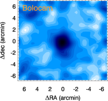
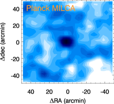
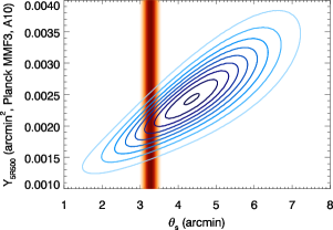
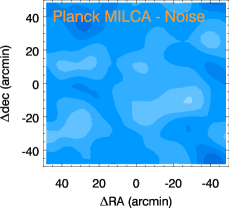
The 2015 Planck data release contains a range of products related to the SZ signal toward clusters, and this analysis utilizes two of those products: 1) the R2.08 cluster catalog created with the MMF3 detection algorithm, which was the baseline catalog for the Planck cluster cosmology analysis (Planck Collaboration et al., 2015c), and 2) the R2.00 all-sky $y$-maps created based on the MILCA algorithm (Planck Collaboration et al., 2015b), which, as detailed below, show good consistency with the MMF3 measurements for the clusters in the BoXSZ⁺ sample.

The MMF3 catalog provides a two-dimensional probability density function (PDF) for each cluster as a function of $Y_{\textrm{5R500}}$ and $\theta_{\textrm{s}}$ assuming an A10 profile. A constraint on $Y_{\textrm{5R500}}$ can therefore be obtained by marginalizing over $\theta_{\textrm{s}}$, either with or without a prior. As an example of such a prior, the MMF3 catalog provides the values of $M_{500}$ derived from the Planck data, based on a scaling relation calibrated using hydrostatic masses from XMM, and these values of $M_{500}$ provide a direct constraint on $\theta_{\textrm{s}}$ for an assumed value of $C_{500}$ (see Figure 1).

In addition to the MMF3 catalog, the value of $Y_{\textrm{5R500}}$ can also be derived using the all-sky MILCA $y$-map by fitting an A10 model directly to the map according to the following procedure. First, a prior on the value of $\theta_{\textrm{s}}$ from the XMM-like measurements is used to set the angular size of the model. Then, the three-dimensional model of the cluster is projected to a two-dimensional image with the line-of-sight projection extending to a radial distance of $5\times R_{500}$. Next, the model is convolved with a $10^{\prime}$ full-width half-maxima (FWHM) Gaussian profile to match the point spread function (PSF) of the MILCA $y$-map, and binned into square pixels with sides of $3.33^{\prime}$. To compare to this candidate model, the full-sky HEALPix MILCA $y$-map data are rebinned into $100^{\prime}\times 100^{\prime}$ thumbnails centered on each cluster with identical $3.33^{\prime}$ square pixels (see Figure 1). Next, 1000 random noise maps are generated from the sum of the inhomogeneous noise map and the full-sky homogeneous noise spectrum under the assumption that the noise is Gaussian. From these noise realizations, a variance per pixel is computed, and the inverse of this variance is used as a weighting factor when fitting the A10 model to the data. The fits are performed using the generalized least squares routine MPFITFUN (Markwardt, 2009), and the only free parameter in the fits is the overall normalization of the A10 model, $Y_{\textrm{5R500}}$.

The homogeneous noise spectrum of the MILCA $y$-map is not white, and therefore the per-pixel variance of the random noise maps does not fully describe the data. As a result, the weighting factors used in the fits are in general sub-optimal. This causes the derived parameter uncertainties from the fits to be larger than those from an optimal fit, but it does not produce any bias in the parameter values. However, the parameter uncertainties will in general be mis-estimated using this procedure. Consequently, rather than estimating these uncertainties using the per-pixel variance, they are determined using the 1000 noise realizations. Specifically, the best-fit model obtained from the data is added to each of the 1000 noise realizations, all of which are then fit using the same procedure as applied to the real data. For each of these fits, the value of $\theta_{\textrm{s}}$ is varied according to its prior, thus fully including these uncertainties. The spread of values obtained for a given parameter based on these 1000 fits then provides the uncertainty on that parameter.

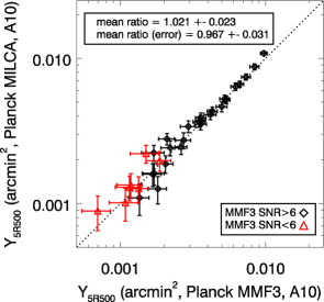
Based on the above fits, the value of $Y_{\textrm{5R500}}$ obtained from the MMF3 catalog is consistent with the value of $Y_{\textrm{5R500}}$ obtained from the MILCA $y$-map, with a sample-mean ratio of $1.021\pm 0.023$ for the 32 BoXSZ⁺ clusters contained in the MMF3 catalog (see Figure 2). Further, the uncertainty on $Y_{\textrm{5R500}}$ is also consistent between the two, with a sample-mean ratio of $0.967\pm 0.031$. Therefore, on average, $Y_{\textrm{5R500}}$ values obtained from fits to the MILCA $y$-maps are equivalent to $Y_{\textrm{5R500}}$ values obtained from the MMF3 catalog.

Figure 2.— Left: the value of $Y_{\textrm{5R500}}$ obtained from A10 fits to the Planck MILCA $y$-maps compared to the value of $Y_{\textrm{5R500}}$ recovered from Planck using the MMF3 algorithm. On average, the two results are consistent. Right: the value of $Y_{\textrm{5R500}}$ obtained from A10 fits to the Bolocam data compared to the value of $Y_{\textrm{5R500}}$ recovered from the Planck MILCA $y$-maps. Given the 5% flux calibration uncertainty on the Bolocam data, the two results are consistent on average. In both plots, clusters above the Planck cluster cosmology cut (MMF3 SNR $>6$) are shown in black, while MMF3 detections below the cut are shown in red. Both plots contain all 32 BoXSZ⁺ clusters detected by Planck using the MMF3 algorithm.

3.3. Bolocam

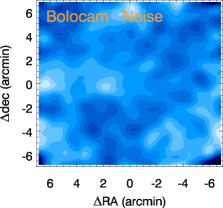
This analysis makes use of the publicly available filtered Bolocam maps, which contain an image of the cluster that has been high-pass filtered according to a two-dimensional transfer function included with the data. Analogous to the MILCA $y$-maps, 1000 noise realizations of the Bolocam maps are provided. The A10 model fits are performed using the same procedure applied to the MILCA $y$-maps, with the following differences: 1) the Bolocam data have a $58^{\prime\prime}$ FWHM PSF, 2) the model must be convolved with the transfer function of the spatial high-pass filter, and 3) the transfer function of the mean signal level of the map is equal to 0, and so an additional nuisance parameter is included in the fits to describe the mean signal.

4. Comparison of SZ Measurements

The Bolocam fit results from Section 3.3 can be directly compared to the Planck-derived results from Section 3.2, which were based on identical A10 model shapes and XMM-like priors on the value of $\theta_{\textrm{s}}$, along with a nearly identical fitting procedure. The weighted mean ratio between the Bolocam and Planck values of $Y_{\textrm{5R500}}$ obtained from these fits is $1.069\pm 0.030$. Given Bolocam’s 5% calibration uncertainty, which is common to all of the clusters and therefore acts as a 5% uncertainty on this average ratio, this result indicates consistency (see Figure 2).

Other groups have also compared Planck SZ measurements to ground-based data. For example, Planck Collaboration et al. (2013a) fit A10 models to a set of 11 clusters using XMM priors on $\theta_{\textrm{s}}$ and SZ data from the Arcminute Microkelvin Imager (AMI). They found an average ratio of $0.95\pm 0.05$ between the values of $Y_{\textrm{5R500}}$ derived from AMI and Planck, indicating good agreement. A later comparison by Perrott et al. (2015), using AMI observations of 99 clusters, found systematically lower values of $Y_{\textrm{5R500}}$ from AMI relative to Planck. However, the value of $\theta_{\textrm{s}}$ was allowed to float in the fits performed in their analysis, and therefore some or all of the difference in $Y_{\textrm{5R500}}$ values may be a result of using different pressure profile shapes when fitting AMI and Planck. More recently, Rodríguez-Gonzálvez et al. (2015) compared SZ measurements from Planck and the Combined Array for Research in Millimeter-wave Astronomy (CARMA-8) for a set of 19 clusters. Like Perrott et al. (2015), they floated the value of $\theta_{\textrm{s}}$ in their fits, although, unlike Perrott et al. (2015), they obtained consistency, with a CARMA-8/Planck ratio of $1.1\pm 0.4$.

5. Joint Fits to Planck and Bolocam and Comparisons to Previous Pressure Profile Results

Motivated by the good agreement between Planck and Bolocam in measuring the value of $Y_{\textrm{5R500}}$ based on identical A10 profile shapes, the data can be combined to jointly constrain a more general gNFW shape. Specifically, given that Bolocam and Planck are most sensitive to the gNFW shape at large radii, the value of the outer logarithmic slope $\beta$ is allowed to vary in these fits while the other parameters are fixed to the A10 values. In order to apply these fits to the largest sample possible, namely the full set of 47 BoXSZ⁺ clusters, an external prior on the value of $\theta_{\textrm{s}}$ is required due to the fact that XMM-like priors only exists for 32 BoXSZ⁺ clusters. This $\theta_{\textrm{s}}$ prior is obtained from previously published values of $M_{500}$ derived using data from Chandra, mainly from Sayers et al. (2013) based on the analysis methods detailed in Mantz et al. (2010). Two BoXSZ⁺ clusters are absent from Sayers et al. (2013), and so the Chandra-derived $M_{500}$ of Abell 1689 is obtained from Mantz et al. (2010) and the Chandra-derived $M_{500}$ of Abell 2744 is obtained from Ehlert et al. (2015).

One subtlety is that the Chandra-derived values of $M_{500}$ are systematically larger than the XMM-like values. In particular, the XMM-like $M_{500}$ values are known to be biased low by $\simeq 30$% compared to lensing masses (von der Linden et al., 2014; Planck Collaboration et al., 2015c), while the Chandra $M_{500}$ values described above are $\simeq 10$% higher than these same lensing masses (Mantz et al., 2014; Applegate et al., 2016). As a result, the XMM-like values of $\theta_{\textrm{s}}$ are smaller than the Chandra values of $\theta_{\textrm{s}}$, with an average ratio of 1.16 for the 32 BoXSZ⁺ clusters in the MMF3 catalog. Since $\theta_{\textrm{s}}$ sets the angular scale of the gNFW profile, this is equivalent to a change in the value of $C_{500}$. However, since $\beta$ is allowed to vary in these fits, and $\beta$ and $C_{500}$ are highly degenerate over the angular scales probed by Planck and Bolocam, this differing choice of $\theta_{\textrm{s}}$ values does not significantly impact the derived profile shape in the radial range where Bolocam and Planck are sensitive, though the specific value of $\beta$ derived from these fits does depend on the choice of $\theta_{\textrm{s}}$ (i.e., of $C_{500}$).

Figure 3.— Best-fit parameters of the joint gNFW fit to Bolocam and Planck. The normalization $P_{0}$ (top row) and outer logarithmic slope $\beta$ (bottom row) were allowed to float, while $C_{\textrm{500}}$, $\alpha$, and $\beta$ were fixed to the A10 values using a prior on $\theta_{\textrm{s}}$ from Chandra. From left to right the plots indicate cluster mass and redshift, with 68% confidence intervals of linear fits from LINMIXERR overlaid in orange. At the median mass of the BoXSZ⁺ sample, the linear fits versus $M_{500}$ provide values of $P_{0}/P_{500}=9.13\pm 0.68\pm 2.98$ and $\beta=6.13\pm 0.16\pm 0.76$.

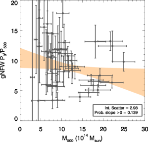
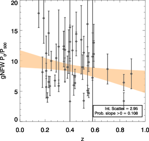
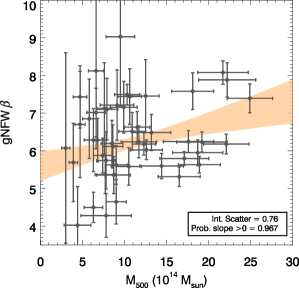
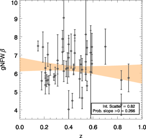
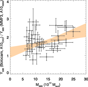
To better understand the results of these jointly constrained gNFW models, linear fits of $P_{0}$ and $\beta$ were performed versus $M_{500}$ and $z$ using LINMIXERR (Kelly, 2007), with the results shown in Figure 3. Only modest correlations exist and the strongest trend is found in $\beta$ versus $M_{500}$. These fits find a cluster-to-cluster scatter of $\simeq 30$% for the value of $P_{0}$ and $\simeq 15$% for the value of $\beta$. If the linear fits versus mass are evaluated at the median value for the BoXSZ⁺ sample, $M_{500}=9.5\times 10^{14}$ M_☉, then the results are $P_{0}/P_{500}=9.13\pm 0.68\pm 2.98$ and $\beta=6.13\pm 0.16\pm 0.76$ (where the first value represents measurement uncertainty and the second indicates intrinsic cluster-to-cluster scatter). Compared to the A10 model, with $P_{0}/P_{500}=8.40$ and $\beta=5.49$, both of these values are slightly larger and indicate a higher pressure in the cluster center with a steeper fall-off at large radius. However, in interpreting these results, it is important to note that, while $\beta$ provides one metric for understanding the pressure profile at large radius, it does not uniquely describe a single shape due to the strong degeneracies between the gNFW parameters. A more robust metric is the ratio between the integrated SZ signal at $R_{500}$ and at $5\times R_{500}$, with Arnaud et al. (2010) obtaining $Y_{500}$/$Y_{\textrm{5R500}}$ $=0.56$. This result can be compared to the value of $Y_{500}$/$Y_{\textrm{5R500}}$$=0.66\pm 0.02\pm 0.10$ obtained from our joint Bolocam/Planck fits to the BoXSZ⁺ clusters (see Table 2).

Table 2gNFW Outer Profile Shapes

Analysis	Data Type	$\beta$	$Y_{500}$/$Y_{\textrm{5R500}}$
this work	SZ observations	6.13	0.66
Le Brun et al. (2015)	simulations	4.63	0.63
Ramos-Ceja et al. (2015)	SZ power spectrum	6.35	0.69
Sayers et al. (2013)	SZ observations	3.67	0.28
Planck Collaboration et al. (2013b)	SZ/X-ray observations	4.13	0.48
Battaglia et al. (2012)	simulations	5.75	0.63
Plagge et al. (2010)	SZ observations	5.50	0.53
Arnaud et al. (2010)	X-ray observations/simulations	5.49	0.56
Nagai et al. (2007)	X-ray observations/simulations	5.00	0.52

Note. — Measurements of the outer pressure profile shape in large samples of clusters. The columns show the reference to the analysis, the type of data used in the analysis, the value of $\beta$, and the value of $Y_{500}$/$Y_{\textrm{5R500}}$. In the case of Le Brun et al. (2015) their “median AGN 8.0” fits were used, and were scaled to the median mass of the BoXSZ⁺ sample using their fitting formulae. In the case of Battaglia et al. (2012), their “AGN Feedback $\Delta=500$” fits were used, and were scaled to the median mass and redshift of the BoXSZ⁺ sample using their fitting formulae. Uncertainties are not available for most analyses, and so they have been omitted.

As mentioned in Section 2.1, a range of other analyses beyond Arnaud et al. (2010) have also constrained gNFW profiles in large samples of clusters. In particular, several groups have examined these profiles at large radius using either simulations or SZ observations. For example, recent simulations from both Kay et al. (2012) and Battaglia et al. (2012) note a trend of increasing $\beta$ with redshift, and both Battaglia et al. (2012) and Le Brun et al. (2015) find increasing values of $\beta$ with increasing mass. Specifically, evaluating the Le Brun et al. (2015) fits at the median mass of the BoXSZ⁺ sample yields $\beta=4.63$ and $Y_{500}$/$Y_{\textrm{5R500}}$ $=0.63$, the latter indicating an outer profile shape that is consistent with our joint Bolocam/Planck fit. Battaglia et al. (2012) used a parameterization allowing $P_{0}$, $\beta$, and $C_{500}$ to vary with mass and redshift according to functional forms described by, for example

$$\beta\propto M^{b_{\textrm{M}}}(1+z)^{b_{\textrm{z}}}.$$

Evaluating their “AGN Feedback $\Delta=500$” fit at the median mass and redshift of the BoXSZ⁺ sample results in a value of $\beta=5.75$ and $Y_{500}$/$Y_{\textrm{5R500}}$ $=0.63$, both in relatively good agreement with our joint Bolocam/Planck fits.

Figure 4.— The ensemble-average best-fit gNFW profile to the joint Bolocam/Planck data for the BoXSZ⁺ sample of clusters (black). Profiles for the 47 individual BoXSZ⁺ clusters are shown as thin gray lines. For comparison, the ensemble-average profiles from other published gNFW fits to large samples of clusters are shown in red (Arnaud et al., 2010), green (Planck Collaboration et al., 2013b), and blue (Sayers et al., 2013). The profiles extend over the approximate radial range probed by the data in each analysis. The ensemble-average profiles show good agreement at $R\lesssim 0.5$$R_{500}$, but noticeably diverge at larger radii.

Given the good agreement of our results with Battaglia et al. (2012), we also fit an identical functional form to the joint Bolocam/Planck constraints on $\beta$, finding $b_{\textrm{M}}=0.077\pm 0.026$ and $b_{\textrm{z}}=-0.06\pm 0.09$. These can be compared to the values of $b_{\textrm{M}}=0.048$ and $b_{\textrm{z}}=0.615$ obtained by Battaglia et al. (2012), although some caution is required because the values of $C_{500}$ were not varied in our fits as they were by Battaglia et al. (2012). These results indicate that the trend in mass seen in the Battaglia et al. (2012) simulations is reproduced in our fits, but the trend in redshift is not.

The lack of a redshift trend could be a result of the BoXSZ⁺ sample selection, which is biased toward relaxed cool-core systems at low-$z$ and toward disturbed merging systems at high-$z$ (see Sayers et al., 2013). For example, 13 BoXSZ⁺ clusters are defined as relaxed based on the SPA criteria of Mantz et al. (2015), and these clusters produce a value of $\beta=6.83\pm 0.37$. In contrast, 10 BoXSZ⁺ clusters are defined as merging based on either failing the Symmetry/Alignment criteria or containing a radio relic/halo based on the analysis of Feretti et al. (2012) and Cassano et al. (2013), and these clusters produce a value of $\beta=5.59\pm 0.61$. Therefore, an excess of cool-core clusters at low-$z$ (which have larger values of $\beta$ on average), and an excess of merging clusters at high-$z$ (which have smaller values of $\beta$ on average), will artificially introduce a trend of decreasing $\beta$ with redshift for the BoXSZ⁺ sample.

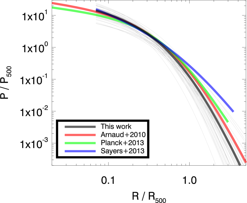
Other groups have used SZ observations to constrain gNFW profile shapes at large radii. For example, Plagge et al. (2010) fit SZ data from a set of 15 clusters, finding $\beta=5.5$ and $Y_{500}$/$Y_{\textrm{5R500}}$ $=0.53$. More recently, Planck Collaboration et al. (2013b) used Planck observations of a larger cluster sample to constrain $\beta=4.13$ and $Y_{500}$/$Y_{\textrm{5R500}}$$=0.48$ (see Table 2 and Figure 4). Both of these analyses indicate a shallower outer profile than our joint Bolocam/Planck fits, although some of this difference may be a result of sample selection. Specifically, the Plagge et al. (2010) sample contains clusters with a median redshift of 0.28 and a median mass of $M_{500}\sim 8\times 10^{14}$ M_☉, and the Planck Collaboration et al. (2013b) sample contains clusters with a median redshift of 0.15 and a median mass of $M_{500}=6.3\times 10^{14}$ M_☉. If the parameterization of Battaglia et al. (2012) is used to rescale their gNFW fits to the median mass and redshift of the BoXSZ⁺ sample, then the resulting value of $Y_{500}$/$Y_{\textrm{5R500}}$ from both the Plagge et al. (2010) and the Planck Collaboration et al. (2013b) fits is equal to 0.56, closer to our value of $0.66\pm 0.02\pm 0.10$. The cause of the remaining difference is unclear, although it could be related to the mass estimates used in these analyses. In particular, Planck Collaboration et al. (2013b) used XMM-derived masses to set the value of $\theta_{500}$, and, as noted above, these masses are known to be biased low, resulting in a different profile shape, and thus $Y_{500}$/$Y_{\textrm{5R500}}$ ratio, for a given set of gNFW parameters.

In another recent work, Sayers et al. (2013) obtained, from a joint fit to Bolocam observations of all the clusters in the BoXSZ sample, $\beta=3.67$ and $Y_{500}$/$Y_{\textrm{5R500}}$ $=0.28$, with an overall profile that noticeably diverges from our joint Bolocam/Planck fit at large radius. This is particularly surprising because the cluster samples are nearly identical, and the only significant difference is the inclusion of Planck data in our current analysis. Because the Bolocam observations were made from the ground at a single observing frequency, they have have reduced sensitivity to large angular scales as a result of both atmospheric fluctuations and primary CMB anisotropies. In contrast, Planck is able to remove CMB anisotropies via its multiple observing channels, and it is not subject to atmospheric fluctuations. Therefore, the Planck data are likely to provide more robust constraints on large angular scales. Though efforts were made in Sayers et al. (2013) to account for the atmospheric and CMB noise, they may be the primary cause of the shallower outer profile found in that work.

Beyond these SZ observations of large samples of individual clusters, Ramos-Ceja et al. (2015) used measurements of the SZ power spectrum on small angular scales from the South Pole Telescope (SPT, Reichardt et al., 2012) to constrain the average pressure profile shape. They found that the A10 model needs to be adjusted to have an outer slope $\beta=6.35\pm 0.19$ ($Y_{500}$/$Y_{\textrm{5R500}}$$=0.69\pm 0.03$) in order to match the SPT measurements. Further, if this value of $\beta$ is adopted, then their analysis implies little or no evolution in its value as a function of redshift. These results are consistent with our findings.

6. Test of the Planck Cluster Completeness Estimate

Figure 5.— The ratio of $Y_{500}$ measured from A10 fits to Bolocam using a Chandra prior on $\theta_{\textrm{s}}$ and $Y_{500}$ measured from the Planck MMF3 algorithm using the A10 model with an XMM-like prior on $\theta_{\textrm{s}}$. The Chandra value of $\theta_{\textrm{s}}$ is larger by an average fraction of 1.16, resulting in systematically larger values of $Y_{500}$ measured by Bolocam. The $Y_{500}$ ratio is shown as a function of $M_{500}$, with the 68% confidence interval of linear fits from LINMIXERR overlaid in orange. This linear fit provides a mapping from the Bolocam measurements of $Y_{500}$ to the Planck measurements of $Y_{500}$, allowing for a test of the Planck completeness using the Bolocam data.

An accurate characterization of the completeness of the Planck cluster survey is required for cosmological analyses, and the discrepancy between the Planck cluster and CMB power spectrum cosmological results motivates special attention to such a characterization (Planck Collaboration et al., 2015c). The details of how the completeness is estimated are given in Planck Collaboration et al. (2015d) and summarized below. First, a set of clusters based on spherical profiles obtained from simulated clusters (Le Brun et al., 2014; McCarthy et al., 2014) are inserted into both real and simulated Planck maps. The MMF3 algorithm is then applied to these maps, and the probability of detecting a cluster above a given SNR is determined as a function of $Y_{500}$ and $\theta_{\textrm{s}}$ based on a brute force Monte-Carlo, which has been publicly released as part of the MMF3 catalog. Ideally, the accuracy of the completeness function would be tested using a catalog of real clusters with known positions, $\theta_{\textrm{s}}$, and $Y_{500}$. In the absence of such a catalog, Planck Collaboration et al. (2015d) undertook a somewhat less demanding test using the MCXC (Piffaretti et al., 2011) and SPT (Bleem et al., 2015) cluster catalogs, which contain cluster positions and $\theta_{\textrm{s}}$ values, but not $Y_{500}$ values.

The BoXSZ⁺ sample enables a better approximation of the ideal test of the Planck completeness because it has positions, $\theta_{\textrm{s}}$, and $Y_{500}$ estimates for each cluster. Specifically, the positions and $\theta_{\textrm{s}}$ values are obtained from Chandra, the latter rescaled by a factor of 1.16 to account for the average difference between the Chandra and XMM values. This rescaling is required because XMM-derived $\theta_{\textrm{s}}$ values were used to calibrate the Planck completeness. Although it would be better to use the XMM $\theta_{\textrm{s}}$ values for all of the BoXSZ⁺ clusters, they only exist for the clusters detected by the MMF3 algorithm, significantly limiting the value of such a test. In order to obtain $Y_{500}$ estimates from Bolocam, the following procedure is applied. First, the Bolocam value of $Y_{500}$ for each BoXSZ⁺ cluster is generated from A10 model fits to the Bolocam data using the Chandra value of $\theta_{\textrm{s}}$. Next, for the 32 BoXSZ⁺ clusters in the MMF3 catalog, the Planck value of $Y_{500}$ is derived from the MMF3 PDF using the XMM-like value of $\theta_{\textrm{s}}$ in order to mimic the computation of $Y_{500}$ values used in the Planck completeness estimate. The ratio of the Bolocam and Planck $Y_{500}$ values is then fit as a function of $M_{500}$ using LINMIXERR (see Figure 5). The results of this linear fit, including the $\simeq 25$% intrinsic scatter, are then used to rescale the Bolocam $Y_{500}$ measurements for all of the BoXSZ⁺ clusters. By fitting versus $M_{500}$, this ensures that the mass dependence of the profile shape found in Section 5 is fully included in the conversion from Bolocam to Planck measurements of $Y_{500}$. As part of this rescaling, an additional 5% uncertainty is added to account for the Bolocam flux calibration uncertainty, although the overall error budget is dominated by the intrinsic scatter in the linear fit.

The Chandra and Bolocam values of $\theta_{\textrm{s}}$ and $Y_{500}$, rescaled to mimic the XMM and Planck values as described in the previous paragraph, are then inserted into the Planck SNR $=6$ completeness estimate to determine a detection probability for each BoXSZ⁺ cluster (see Figure 6). One subtlety is that the noise in the Planck maps is not uniform over the full sky, and it is therefore necessary to account for this variation when calculating the detection probability for each BoXSZ⁺ cluster. Specifically, this variation is accounted for by comparing the noise RMS within the MILCA $y$-map thumbnail centered on each cluster to the average noise RMS within the region of sky satisfying the cuts used for the Planck cluster analysis. In general, the local noise is within 5% of the average, and the most extreme local noise deviation is 12%.

Figure 6.— Left: The probability for each BoXSZ⁺ cluster to be detected with SNR $>6$ by Planck using the MMF3 algorithm in ascending order of detection probability. The probability is computed using the Bolocam measurement of $Y_{\textrm{5R500}}$, rescaled according to the linear fit shown in Figure 5. Black diamonds denote the clusters actually detected by Planck and red triangles denote non-detections. The vertical bars represent the range of probabilities predicted from the Bolocam measurement of $Y_{\textrm{5R500}}$, with most of the uncertainty due to the intrinsic scatter in the linear model used to rescale the Bolocam measurements. Right: 68% (dark orange) and 95% (light orange) confidence regions for the total cumulative number of Planck MMF3 clusters with SNR $>6$ based on the detection probabilities given in the left plot. The actual cumulative number of Planck detections is given as a solid black line, and is consistent with, but somewhat low, compared to the predictions based on Bolocam.

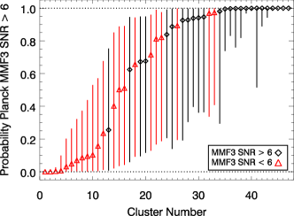
The left panel of Figure 6 shows the probability for every BoXSZ⁺ cluster to be detected by the Planck MMF3 algorithm with a $\textrm{SNR}>6$. There are no obvious outliers, with Planck detecting all of the clusters with a probability of $\sim 1$ and none of the clusters with a probability of $\sim 0$. To provide a quantitative test, a simulation was performed based on the estimated detection probabilities. For each run of the simulation, a random value was drawn for each BoXSZ⁺ cluster based on the detection probability distribution for that cluster, and the total cumulative number of detections was computed. The simulation was repeated 10000 times, and the resulting 68% and 95% confidence regions on the cumulative detections are plotted in the right panel of Figure 6. The average number of detections in the simulations is 27.6, and 16% of the simulations result in fewer than the actual number of clusters detected by Planck, which is 25.

This result provides a more extensive validation of the Planck completeness estimate, although Planck does detect slightly fewer clusters than expected given the Bolocam $Y_{500}$ measurements. Such a shortfall could partially explain the tension seen between the CMB-derived and cluster-derived cosmological constraints (Planck Collaboration et al., 2015c, a). For example, Planck Collaboration et al. (2015c) quantifies the level of tension in terms of a cluster mass bias, with a value of $(1-b)=0.58$ required to forge agreement. This is smaller than the true mass bias, with $(1-b)\simeq 0.7$–$0.8$ found from lensing-based mass calibrations (Planck Collaboration et al., 2015c; von der Linden et al., 2014; Hoekstra et al., 2015), and the remaining 10–20% difference is not well understood. Following this convention, the discrepancy between the predicted and actual number of Planck detections from the BoXSZ⁺ sample can be recast as an effective mass bias. In order for the average number of predicted detections to equal the actual number of 25, the Bolocam $Y_{500}$ measurements would need to be lower by a factor of $0.88\pm 0.11$. Based on the $Y_{500}$/$M_{500}$ scaling relation derived in Planck Collaboration et al. (2014), this corresponds to an effective mass bias factor of $(1-b)=0.93\pm 0.06$. This effective bias is multiplicative with the true mass bias, and would bring the Planck cluster results into better agreement with the Planck CMB results.

7. Summary

We fit A10 models to the Planck MILCA $y$-maps using an XMM-like prior on the value of $\theta_{\textrm{s}}$, obtaining $Y_{\textrm{5R500}}$ values consistent with those determined from the Planck MMF3 algorithm using the same $\theta_{\textrm{s}}$ prior. We also derived $Y_{\textrm{5R500}}$ from ground-based Bolocam observations, finding a Bolocam/Planck $Y_{\textrm{5R500}}$ ratio of of $1.069\pm 0.030$. This value is consistent with unity given calibration uncertainties and implies that Bolocam and Planck measure consistent SZ signals. Our results are in good agreement with previous comparisons between Planck and the ground-based AMI and CARMA-8 receivers, which yielded similar consistency

We also performed joint fits to the Bolocam and Planck data, using a gNFW model with the outer logarithmic slope $\beta$ allowed to vary with the other shape parameters fixed to the A10 values. These fits produce average values of $\beta=6.13\pm 0.16\pm 0.76$ and $Y_{500}$/$Y_{\textrm{5R500}}$ $=0.66\pm 0.02\pm 0.10$, which are in good agreement with recent simulations for clusters matching the masses and redshifts of the BoXSZ⁺ sample. Compared to simulations, our data are also consistent with the trend of increasing $\beta$ with increasing cluster mass, but they do not reproduce the relatively strong trend of increasing $\beta$ with increasing redshift, likely due to selection effects in the BoXSZ⁺ sample. Previous SZ measurements of $\beta$ and $Y_{500}$/$Y_{\textrm{5R500}}$ indicate lower values than our results, although some or all of this difference may be due to a combination of different median masses and redshifts within those samples, different mass measurements used to set the cluster radial scale, and/or measurement noise.

Using Bolocam measurements of $Y_{500}$ and Chandra measurements of $\theta_{\textrm{s}}$, both rescaled to account for systematic differences relative to Planck measurements of $Y_{500}$ and XMM measurements of $\theta_{\textrm{s}}$, we compute the detection probability for each BoXSZ⁺ cluster using the publicly available Planck completeness estimate. We estimate that Planck should detect an average of 27.6 BoXSZ⁺ clusters above the MMF3 SNR limit for the cosmology sample, a value that is within $\simeq 1\sigma$ of the actual number of Planck detections, which is 25. Our results therefore provide a further validation of the Planck completeness estimate. Taking the small discrepancy at face value, however, may suggest that Planck detects fewer clusters than expected. Translated to an effective mass bias, this discrepancy yields $(1-b)=0.93\pm 0.06$. This effective mass bias is multiplicative with the true mass bias of $(1-b)\simeq 0.7$–0.8 determined from lensing measurements, and would partially account for the difference between the Planck cluster-derived and CMB-derived cosmological parameters that has not been explained by the lensing measurements (Planck Collaboration et al., 2015a, c).

8. Acknowledgments

We acknowledge the assistance of: Kathy Deniston, who provided effective administrative support at Caltech; James Bartlett and Jean-Baptiste Melin, who provided useful discussions; JS was supported by a NASA/ADAP award; MN, GP, and BW were supported by the Caltech Summer Research Connection program. SRS was supported by a NASA Earth and Space Science Fellowship and a generous donation from the Gordon and Betty Moore Foundation.

Facilities: Caltech Submillimeter Observatory, Planck, Chandra.

References

- Adam et al. (2016) Adam, R., Comis, B., Bartalucci, I., et al. 2016, A&A, 586, A122
- Applegate et al. (2016) Applegate, D. E., Mantz, A., Allen, S. W., et al. 2016, MNRAS, 457, 1522
- Arnaud et al. (2010) Arnaud, M., Pratt, G. W., Piffaretti, R., et al. 2010, A&A, 517, A92
- Babyk et al. (2012) Babyk, I., Melnyk, O., & Elyiv, A. 2012, Advances in Astronomy and Space Physics, 2, 188
- Battaglia et al. (2012) Battaglia, N., Bond, J. R., Pfrommer, C., & Sievers, J. L. 2012, ApJ, 758, 75
- Benson et al. (2004) Benson, B. A., Church, S. E., Ade, P. A. R., et al. 2004, ApJ, 617, 829
- Birkinshaw (1999) Birkinshaw, M. 1999, Phys. Rep., 310, 97
- Bleem et al. (2015) Bleem, L. E., Stalder, B., de Haan, T., et al. 2015, ApJS, 216, 27
- Cassano et al. (2013) Cassano, R., Ettori, S., Brunetti, G., et al. 2013, ApJ, 777, 141
- Chluba et al. (2012) Chluba, J., Nagai, D., Sazonov, S., & Nelson, K. 2012, MNRAS, 426, 510
- Czakon et al. (2015) Czakon, N. G., Sayers, J., Mantz, A., et al. 2015, ApJ, 806, 18
- Ehlert et al. (2015) Ehlert, S., Allen, S. W., Brandt, W. N., et al. 2015, MNRAS, 446, 2709
- Feretti et al. (2012) Feretti, L., Giovannini, G., Govoni, F., & Murgia, M. 2012, A&A Rev., 20, 54
- Hasselfield et al. (2013) Hasselfield, M., Hilton, M., Marriage, T. A., et al. 2013, JCAP, 7, 008
- Hoekstra et al. (2015) Hoekstra, H., Herbonnet, R., Muzzin, A., et al. 2015, MNRAS, 449, 685
- Itoh et al. (1998) Itoh, N., Kohyama, Y., & Nozawa, S. 1998, ApJ, 502, 7
- Itoh & Nozawa (2004) Itoh, N., & Nozawa, S. 2004, A&A, 417, 827
- Kay et al. (2012) Kay, S. T., Peel, M. W., Short, C. J., et al. 2012, MNRAS, 422, 1999
- Kelly (2007) Kelly, B. C. 2007, ApJ, 665, 1489
- Kitayama et al. (2004) Kitayama, T., Komatsu, E., Ota, N., et al. 2004, PASJ, 56, 17
- Le Brun et al. (2015) Le Brun, A. M. C., McCarthy, I. G., & Melin, J.-B. 2015, MNRAS, 451, 3868
- Le Brun et al. (2014) Le Brun, A. M. C., McCarthy, I. G., Schaye, J., & Ponman, T. J. 2014, MNRAS, 441, 1270
- Mantz et al. (2010) Mantz, A., Allen, S. W., Ebeling, H., Rapetti, D., & Drlica-Wagner, A. 2010, MNRAS, 406, 1773
- Mantz et al. (2014) Mantz, A. B., Allen, S. W., Morris, R. G., et al. 2014, MNRAS, 440, 2077
- Mantz et al. (2016) Mantz, A. B., Allen, S. W., Morris, R. G., & Schmidt, R. W. 2016, MNRAS, 456, 4020
- Mantz et al. (2015) Mantz, A. B., Allen, S. W., Morris, R. G., et al. 2015, MNRAS, 449, 199
- Markwardt (2009) Markwardt, C. B. 2009, in Astronomical Society of the Pacific Conference Series, Vol. 411, Astronomical Data Analysis Software and Systems XVIII, ed. D. A. Bohlender, D. Durand, & P. Dowler, 251
- Mason et al. (2010) Mason, B. S., Dicker, S. R., Korngut, P. M., et al. 2010, ApJ, 716, 739
- Mauskopf et al. (2012) Mauskopf, P. D., Horner, P. F., Aguirre, J., et al. 2012, MNRAS, 421, 224
- McCarthy et al. (2014) McCarthy, I. G., Le Brun, A. M. C., Schaye, J., & Holder, G. P. 2014, MNRAS, 440, 3645
- McDonald et al. (2014) McDonald, M., Benson, B. A., Vikhlinin, A., et al. 2014, ApJ, 794, 67
- Nagai et al. (2007) Nagai, D., Kravtsov, A. V., & Vikhlinin, A. 2007, ApJ, 668, 1
- Navarro et al. (1997) Navarro, J. F., Frenk, C. S., & White, S. D. M. 1997, ApJ, 490, 493
- Nozawa et al. (1998) Nozawa, S., Itoh, N., & Kohyama, Y. 1998, ApJ, 507, 530
- Perrott et al. (2015) Perrott, Y. C., Olamaie, M., Rumsey, C., et al. 2015, A&A, 580, A95
- Piffaretti et al. (2011) Piffaretti, R., Arnaud, M., Pratt, G. W., Pointecouteau, E., & Melin, J.-B. 2011, A&A, 534, A109
- Plagge et al. (2010) Plagge, T., Benson, B. A., Ade, P. A. R., et al. 2010, ApJ, 716, 1118
- Planck Collaboration et al. (2013a) Planck Collaboration, AMI Collaboration, Ade, P. A. R., et al. 2013a, A&A, 550, A128
- Planck Collaboration et al. (2013b) Planck Collaboration, Ade, P. A. R., Aghanim, N., et al. 2013b, A&A, 550, A131
- Planck Collaboration et al. (2014) —. 2014, A&A, 571, A20
- Planck Collaboration et al. (2015a) —. 2015a, ArXiv e-prints, arXiv:1502.01589
- Planck Collaboration et al. (2015b) Planck Collaboration, Aghanim, N., Arnaud, M., et al. 2015b, ArXiv e-prints, arXiv:1502.01596
- Planck Collaboration et al. (2015c) Planck Collaboration, Ade, P. A. R., Aghanim, N., et al. 2015c, ArXiv e-prints, arXiv:1502.01597
- Planck Collaboration et al. (2015d) —. 2015d, ArXiv e-prints, arXiv:1502.01598
- Ramos-Ceja et al. (2015) Ramos-Ceja, M. E., Basu, K., Pacaud, F., & Bertoldi, F. 2015, A&A, 583, A111
- Reese et al. (2012) Reese, E. D., Mroczkowski, T., Menanteau, F., et al. 2012, ApJ, 751, 12
- Reichardt et al. (2012) Reichardt, C. L., Shaw, L., Zahn, O., et al. 2012, ApJ, 755, 70
- Rephaeli (1995) Rephaeli, Y. 1995, ApJ, 445, 33
- Rodríguez-Gonzálvez et al. (2015) Rodríguez-Gonzálvez, C., Chary, R., Muchovej, S., et al. 2015, ArXiv e-prints, arXiv:1505.01132
- Romero et al. (2015) Romero, C. E., Mason, B. S., Sayers, J., et al. 2015, ApJ, 807, 121
- Sayers et al. (2013) Sayers, J., Czakon, N. G., Mantz, A., et al. 2013, ApJ, 768, 177
- Sayers et al. (2016) Sayers, J., Zemcov, M., Glenn, J., et al. 2016, ApJ, 820, 101
- Sunyaev & Zeldovich (1980) Sunyaev, R. A., & Zeldovich, I. B. 1980, MNRAS, 190, 413
- Sunyaev & Zel’dovich (1972) Sunyaev, R. A., & Zel’dovich, Y. B. 1972, Comments on Astrophysics and Space Physics, 4, 173
- von der Linden et al. (2014) von der Linden, A., Mantz, A., Allen, S. W., et al. 2014, MNRAS, 443, 1973
- Young et al. (2015) Young, A. H., Mroczkowski, T., Romero, C., et al. 2015, ApJ, 809, 185
- Zemcov et al. (2010) Zemcov, M., Rex, M., Rawle, T. D., et al. 2010, A&A, 518, L16