Compact Hash Codes for Efficient Visual Descriptors Retrieval in Large Scale Databases
Abstract
In this paper we present an efficient method for visual descriptors retrieval based on compact hash codes computed using a multiple k-means assignment. The method has been applied to the problem of approximate nearest neighbor (ANN) search of local and global visual content descriptors, and it has been tested on different datasets: three large scale public datasets of up to one billion descriptors (BIGANN) and, supported by recent progress in convolutional neural networks (CNNs), also on the CIFAR-10 and MNIST datasets. Experimental results show that, despite its simplicity, the proposed method obtains a very high performance that makes it superior to more complex state-of-the-art methods.
1 Introduction
Efficient nearest neighbor (NN) search is one of the main issues in large scale information retrieval for multimedia and computer vision tasks. When dealing with high dimensional features also methods for multidimensional indexing obtain performance comparable to that of exhaustive search [17]. A typical solution is to employ methods that perform approximate nearest neighbor (ANN) search, typically using feature hashing and Hamming distances. These methods generally use inverted files, e.g. implemented using hash tables, and require to use hash codes with a length of several tens of bits to obtain a reasonable performance in retrieval. This combination requires quite large amounts of memory to store large scale databases of features, thus their application to systems with relatively limited memory (e.g. mobile devices still have 1-2 GB RAM only) or systems that involve a large-scale media analysis is not feasible.
In this paper we present a novel method for feature hashing, based on multiple k-means assignments, that is unsupervised, that requires a very limited codebook size and that obtains good performance in retrieval even with very compact hash codes. The proposed approach greatly reduces the need of training data and memory requirements for the quantizer, and obtains a retrieval performance similar or superior to more complex state-of-the-art approaches on standard large scale datasets. This makes it suitable, in terms of computational cost, for mobile devices, large-scale media analysis and retrieval in general.
2 Previous Works
Previous works on visual feature hashing can be divided in methods based on hashing functions, scalar quantization, vector quantization and, more recently, neural networks.
Hashing functions
Weiss et al.[36] have proposed to treat the problem of hashing as a particular form of graph partitioning, in their Spectral Hashing algorithm.
Heo et al.[14] have proposed to encode high-dimensional data points using hyperspheres instead of hyperplanes; Jin et al.[20] have proposed a variation of LSH, called Density Sensitive Hashing, that does not use random projections but instead uses projective functions that are more suitable for the distribution of the data.
Du et al.[8] have proposed the use of Random Forests to perform linear projections, along with a metric that is not based on Hamming distance.
Paulevé et al.[32] have compared structured quantization algorithms with structured quantizers (i.e. k-means and hierarchical k-means clustering). Experimental results on SIFT descriptors have shown that unstructured quantizers provide significantly superior performances with respect to structured quantizers.
Scalar Quantization
Zhou et al.[39] have proposed an approach based on scalar quantization of SIFT descriptors. The median and the third quartile of the bins of the descriptor are computed and used as thresholds, hashing is then computed coding the value of each bin of the descriptor with 2 bits, depending on this subdivision. The final hash code has a dimension of 256 bits, but only the first 32 bits are used to index the code in an inverted file. The method of [39] has been extended by Ren et al.[33], including an evaluation of the reliability of bits, depending on their quantization errors. Unreliable bits are then flipped when performing search, as a form of query expansion. Chen and Hsieh [6] have recently proposed an approach that quantizes the differences of the bins of the SIFT descriptor, using the median computed on all the SIFT descriptors of a training set as a threshold.
Vector Quantization
Jégou et al.[17] have proposed to decompose the feature space into a Cartesian product of subspaces with lower dimensionality, that are quantized separately. This Product Quantization (PQ) method is efficient in solving memory issues that arise when using vector quantization methods such as k-means, since it requires a much reduced number of centroids. The method has obtained state-of-the-art results on a large scale SIFT features dataset, improving over methods such as SH [36] and Hamming Embedding [15]. This result is confirmed in the work of Chandrasekhar et al.[4], that have compared several compression schemes for SIFT features.
The success of the Product Quantization method has led to development of several variations and improvements. The idea of compositionality of the PQ approach has been further analyzed by Norouzi and Fleet [29], that have built upon it proposing two variations of k-means: Orthogonal k-means and Cartesian k-means. Also Ge et al.[9] have proposed another improvement of PQ, called OPQ, that minimizes quantization distortions w.r.t. space decomposition and quantization codebooks; He et al.[13] have proposed an affinity-preserving technique to approximate the Euclidean distance between codewords in k-means method. Kalantidis and Avrithis [21] have presented a simple vector quantizer (LOPQ) which uses a local optimization over a rotation and a space decomposition and apply a parametric solution that assumes a normal distribution.
Babenko and Lempitsky [2] have proposed an efficient similarity search method, called inverted multi-index (Multi-D-ADC); this approach generalizes the inverted index by replacing vector quantization inside inverted indices with product quantization, and building the multi-index as a multi-dimensional table.
Neural Networks
Lin et al.[27] have proposed a deep learning framework to create hash-like binary codes for fast image retrieval. Hash codes are learned in a point-wise manner by employing a hidden layer for representing the latent concepts that dominate the class labels (when the data labels are available). This layer learns specific image representations and a set of hash-like functions.
Do et al.[7] have addressed the problem of learning binary hash codes for large scale image search using a deep model which tries to preserve similarity, balance and independence of images. Two sub-optimizations during the learning process allow to efficiently solve binary constraints.
Guo and Li [12] have proposed a method to obtain the binary hash code of a given image using binarization of the CNN outputs of a certain fully connected layer.
Zhang et al.[38] have proposed a very deep neural networks (DNNs) model for supervised learning of hash codes (VDSH). They use a training algorithm inspired by alternating direction method of multipliers (ADMM) [3]. The method decomposes the training process into independent layer-wise local updates through auxiliary variables.
Xia et al.[37] have proposed an hashing method for image retrieval which simultaneously learns a representation of images and a set of hash functions.
3 The Proposed Method
The proposed method exploits a novel version of the k-means vector quantization approach, introducing the possibility of assignment of a visual feature to multiple cluster centers during the quantization process. This approach greatly reduces the number of required cluster centers, as well as the required training data, performing a sort of quantized codebook soft assignment for an extremely compact hash code of visual features.
The first step of the computation is a typical k-means algorithm for clustering. Given a set of observations where each observation is a d-dimensional real vector, k-means clustering partitions the observations into sets so as to minimize the sum of distance functions of each point in the cluster to the centers. Its objective is to find:
| (1) |
This process is convergent (to some local optimum) but the quality of the local optimum strongly depends on the initial assignment. We use the k-means++ [1] algorithm for choosing the initial values, to avoid the poor clusterings sometimes found by the standard k-means algorithm.
3.1 Multi-k-means Hashing
K-means is typically used to compute the hash code of visual feature in unstructured vector quantization, because it minimizes the quantization error by satisfying the two Lloyd optimality conditions [17]. In a first step a dictionary is learned over a training set and then hash codes of features are obtained by computing their distance from each cluster center. Vectors are assigned to the nearest cluster center, whose code is used as hash code. Considering the case of 128-dimensional visual content descriptors like SIFT or the FC7 layer of the VGG-M-128 CNN [5], this means that compressing them to 64 bits codes requires to use centroids. In this case the computational cost of learning a k-means based quantizer becomes expensive in terms of memory and time because: i) there is the need of a quantity of training data that is several times larger than , and ii) the execution time of the algorithm becomes unfeasible. Using hierarchical k-means (HKM) makes it possible to reduce execution time, but the problem of memory usage and size of the required learning set affect also this approach. Since the quantizer is defined by the centroids, the use of quantizers with a large number of centroids may not be practical or efficient: if a feature has a dimension , there is need to store values to represent the codebook of the quantizer. A possible solution to this problem is to reduce the length of the hash signature, but this typically affects negatively retrieval performance. The use of product k-means quantization, proposed originally by Jégou et al.[17], overcomes this issue.
In our approach, instead, we propose to compute a sort of soft assignment within the k-means framework, to obtain very compact signatures and dimension of the quantizer, thus reducing its memory requirements, while maintaining a retrieval performance similar to that of [17].
The proposed method, called multi-k-means, starts learning a standard k-means dictionary as shown in Eq. 1, using a very small number of centroids to maintain a low computational cost. Once we obtained our centroids, the main difference resides in the assignment and creation of the hash code. Each centroid is associated to a specific bit of the hash code:
| (2) |
where is the feature point and is a threshold measure given by
| (3) |
i.e. centroid is associated to the bit of the hash code of length ; the bit is set to if the feature to be quantized is assigned to its centroid, or to otherwise.
A feature can be assigned to more than one centroid using two different approaches:
i) m-k-means-t - using Eq. (2) and one of the first two thresholds of Eq. (3). In this case the feature vector is considered as belonging to all the centroids from which its distance is below the threshold. Experiments have shown that the arithmetic mean is more efficient with respect to the geometric one, and all the experiments will report results obtained with it.
ii) m-k-means-n - using Eq. (2) and the third threshold of Eq. (3), i.e. assigning the feature to a predefined number of nearest centroids.
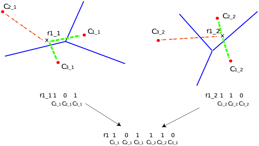
We also introduce a variant (m-k-means-t2 and m-k-means-n2) to the previous approaches by randomly splitting the training data into two groups and creating two different codebooks for each feature vector. The final hash code is given by the union of these two codes.
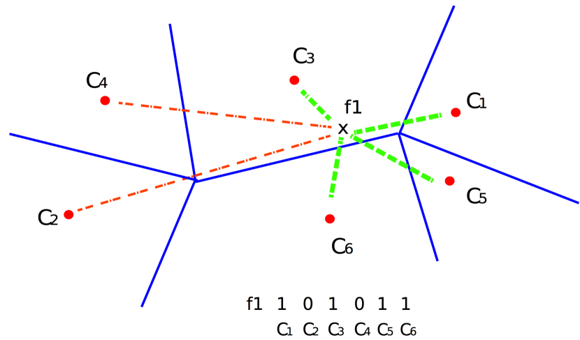
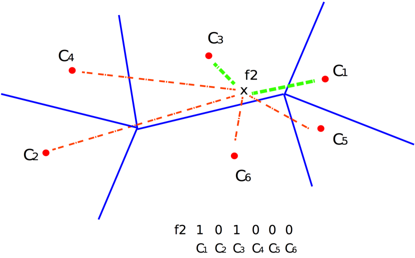
With the proposed approach it is possible to create hash signatures using a much smaller number of centroids than using the usual k-means baseline, since each centroid is directly associated to a bit of the hash code. This approach can be considered a quantized version of codebook soft assignment [35] and, similarly, it alleviates the problem of codeword ambiguity while reducing the quantization error.
Fig. 1 illustrates the quantization process and the resulting hash codes in three cases: one in which a vector is assigned to a variable number of centroids (m-k-means-t), one in which a vector is assigned to a predefined number of centroids (m-k-means-n) and one in which the resulting code is created by the union of two different codes created using two different codebooks (m-k-means-x2, where can be either or ). In all cases the feature is assigned to more than one centroid. An evaluation of these two approaches is reported in Sect. 4.
Typically a multi probe approach is used to solve the problem of ambiguous assignment to a codebook centroid (in case of vector quantization) or quantization error (e.g. in case of scalar quantization). With this approach one or more bits of the query hash code are flipped to perform a query expansion, improving recall at the expense of computational cost and search time. In the proposed method this need of multi probe queries is greatly reduced, because of the possibility of assignment of features to more than one centroid. In fact, all the experiments have been performed without using multi probe querying.
4 Experimental results
The variants of the proposed method (m-k-means-t, m-k-means-n, m-k-means-t2 and m-k-means-n2) have been thoroughly compared to several state-of-the-art approaches using standard datasets, experimental setups and evaluation metrics.
4.1 Datasets
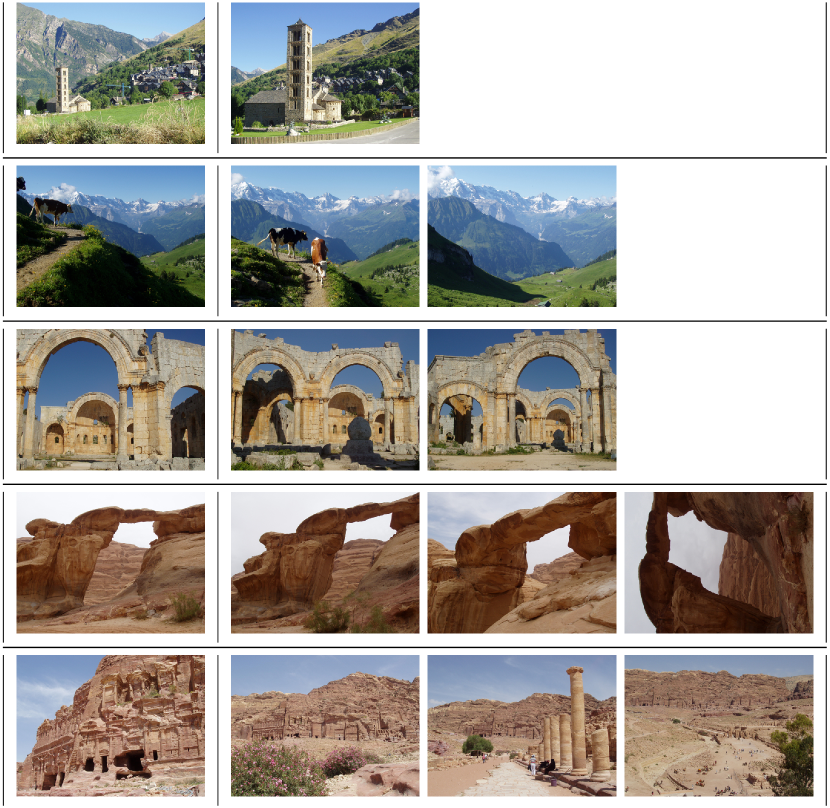
BIGANN Dataset [18, 17] is a large-scale dataset commonly used to compare methods for visual feature hashing and approximate nearest neighbor search [18, 17, 2, 31, 29, 21, 9]. The dataset is composed by three different sets of SIFT and GIST descriptors, each one divided in three subsets: a learning set, a query set and base set; each query has corresponding ground truth results in the base set, computed in an exhaustive way with Euclidean distance, ordered from the most similar to the most different. For SIFT1M and SIFT1B query and base descriptors have been extracted from the INRIA Holidays images [16], while the learning set has been extracted from Flickr images. For GIST1M query and base descriptors are from INRIA Holidays and Flickr 1M datasets, while learning vectors are from [34]. In all the cases query descriptors are from the query images of INRIA Holidays (see Figure 2). The characteristics of the dataset are summarized in Table 1.
| vector dataset | SIFT 1M | SIFT 1B | GIST 1M |
|---|---|---|---|
| descriptor dimensionality | 128 | 128 | 960 |
| # learning set vectors | 100,000 | 100,000,000 | 500,000 |
| # database set vectors | 1,000,000 | 1,000,000,000 | 1,000,000 |
| # queries set vectors | 10,000 | 10,000 | 1,000 |
| # nearest vectors for each query | 100 | 1000 | 100 |
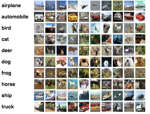
CIFAR-10 Dataset [22] consists of 60,000 colour images ( pixels) in 10 classes, with 6,000 images per class (see Figure 3). The dataset is split into training and test sets, composed by 50,000 and 10,000 images respectively. A retrieved image is considered relevant for the query if it belongs to the same class. This dataset has been used for ANN retrieval in [37, 27].
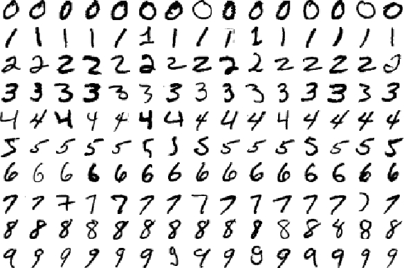
MNIST Dataset [26] consists of 70,000 handwritten digits images ( pixels, see Figure 4). The dataset is split into 60,000 training examples and 10,000 test examples. Similarly to CIFAR-10 a retrieved image is considered relevant if it belongs to the same class of the query. This dataset has been used for ANN retrieval in [37, 27].
4.2 Evaluation Metrics
The performance of ANN retrieval in BIGANN dataset is evaluated using recall@R, which is used in most of the results reported in the literature [17, 18, 29, 21, 9, 2] and it is, for varying values of R, the average rate of queries for which the 1-nearest neighbor is retrieved in the top R positions. In case of this metric coincides with precision@1.
Performance of image retrieval in CIFAR-10 and MNIST is measured following the setup of [37], using Mean Average Precision:
| (4) |
where
| (5) |
is the area under the precision-recall curve and is the number of queries.
4.3 Configurations and Implementations
BIGANN
We use settings which reproduce top performances at 64-bit codes. We perform search with a non-exhaustive approach. For each query 64 bits binary hash code of the feature and Hamming distance measure are used to extract small subsets of candidate from the whole database set (Table 1). Euclidean distance measure is then used to re-rank the nearest feature points, calculating recall@R values in these subsets.
CIFAR-10
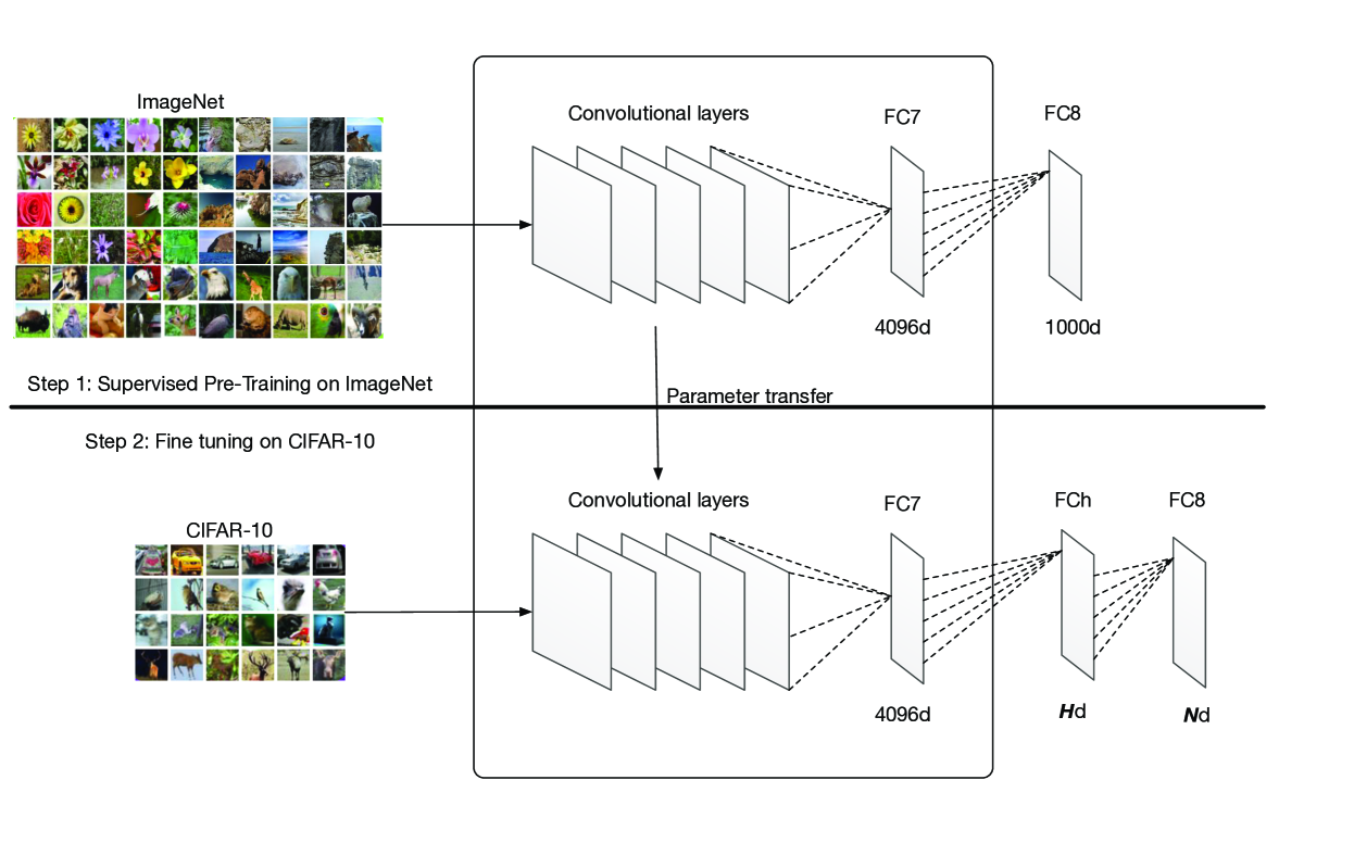
We use features computed with the framework proposed in [27] (Figure 5). The process is carried out in two steps: in the first step a supervised pre-training on the large-scale ImageNet dataset [23] is performed. In the second step fine-tuning of the network is performed, with the insertion of a latent layer that simultaneously learns domain specific feature representations and a set of hash-like functions. The authors used the pre-trained CNN model proposed by Krizhevsky et al.[23] and implemented in the Caffe CNN library [19]. In our experiments we use features coming from the Layer (Latent Layer H), which has a size of 48 nodes.
MNIST
We use LeNet CNN to compute our features in MNIST. This is a network architecture developed by LeCun [25] that was especially designed for recognizing handwritten digits, reading zip codes, etc. It is a 8-layer network with 1 input layer, 2 convolutional layers, 2 non-linear down-sampling layers, 2 fully connected layers and a Gaussian connected layer with 10 output classes. We used a modified version of LeNet [19] and we obtain features from the first fully connected layer.
We perform search with a non-exhaustive approach on both CIFAR-10 and MNIST datasets. For each image we extract a 48-dimensional feature vector for CIFAR-10, and 500-dimensional feature vector for MNIST, from the respective network and then we generate a 48 bits binary hash code using the proposed methods of Sect. 3. Hamming distance is used to select the nearest hash codes for each query and similarity measure given by
| (6) |
where and are the components of the original feature vectors and , is used to re-rank the nearest visual features.
4.4 Results on BIGANN: SIFT1M, GIST1M
In this set of experiments the proposed approach and its variants are compared on the SIFT1M (Table 2) and GIST1M (Table 3) datasets against four methods discussed in section 2: Product Quantization (ADC and IVFADC)[17], Cartesian k-means [29], LOPQ [21] and a non-exhaustive adaptation of OPQ [9], called I-OPQ [21].
ADC (Asymmetric Distance Computation) is characterized by the number of sub vectors m and the number of quantizers per sub vectors , and produces a code of length m . IVFADC (Inverted File with Asymmetric Distance Computation) is characterized by the codebook size (number of centroids associated to each quantizer), the number of neighbouring cells w visited during the multiple assignment, the number of sub vectors m and the number of quantizers per sub vectors which is in this case fixed to . The length of the final code is given by m .
Cartesian k-means (ck-means) [29] models region center as an additive combinations of subcenters. Let be the number of subcenters, with elements, then the total number of model centers is , but the total number of subcenters is , and the number of bits of the signature is .
LOPQ (The Locally optimized product quantization) [21] is a vector quantizer that combines low distortion with fast search applying a local optimization over rotation and space decomposition.
I-OPQ [21] is a non-exhaustive adaptation of OPQ (Optimized Product Quantization) [9] which use either OPQP or OPQNP global optimization.
The parameters of the proposed methods are set as follows: for m-k-means-t we use as threshold the arithmetic mean of the distances between feature vectors and centroids to compute hash code; m-k-means-n creates hash code by setting to 1 the corresponding position of the first 32 (SIFT1M) and first 48 (GIST1M) nearest centroids for each feature; m-k-means-t2 and m-k-means-n2 create two different sub hash codes for each feature by splitting into two parts the training phase and combine these two sub parts into one single code to create the final signature. Since we have a random splitting during the training phase, these experiments are averaged over a set of 10 runs.
| method | R@1 | R@10 | R@100 | R@1000 | R@10000 |
| ADC [17] | 0.224 | 0.600 | 0.927 | 0.996 | 0.999 |
| IVFADC [17] | 0.320 | 0.739 | 0.953 | 0.972 | 0.972 |
| ck-means [29] | 0.231 | 0.635 | 0.930 | 1 | 1 |
| I-OPQ [21] | 0.299 | 0.691 | 0.875 | 0.888 | 0.888 |
| LOPQ [21] | 0.380 | 0.780 | 0.886 | 0.888 | 0.888 |
| m-k-means-t | 0.501 | 0.988 | 1 | 1 | 1 |
| m-k-means-t2 | 0.590 | 0.989 | 1 | 1 | 1 |
| m-k-means-n | 0.436 | 0.986 | 1 | 1 | 1 |
| m-k-means-n2 | 0.561 | 0.986 | 1 | 1 | 1 |
| method | R@1 | R@10 | R@100 | R@1000 | R@10000 |
| ADC[17] | 0.145 | 0.315 | 0.650 | 0.932 | 0.997 |
| IVFADC[17] | 0.180 | 0.435 | 0.740 | 0.966 | 0.992 |
| ck-means[29] | 0.135 | 0.335 | 0.728 | 0.952 | 0.985 |
| I-OPQ[21] | 0.146 | 0.410 | 0.729 | 0.862 | 0.866 |
| LOPQ[21] | 0.160 | 0.461 | 0.756 | 0.860 | 0.866 |
| m-k-means-t | 0.111 | 0.906 | 1 | 1 | 1 |
| m-k-means-t2 | 0.123 | 0.890 | 1 | 1 | 1 |
| m-k-means-n | 0,231 | 0,940 | 1 | 1 | 1 |
| m-k-means-n2 | 0,265 | 0,905 | 1 | 0,999 | 0,999 |
The proposed method obtains the best results when considering the more challenging values of recall@R, i.e. with a small number of nearest neighbors, like 1, 10 and 100. When R goes to 1000 and 10,000 it still obtains the best results and in the case of SIFT1M it is on par with ck-means [29]. Considering GIST1M the method consistently outperforms all the other methods for all the values of R.
4.5 Results on BIGANN: SIFT1B
In this experiment we compare our method on the SIFT1B dataset (Table 4) against LOPQ and a sub-optimal variant LOR+PQ [21], a single index approaches IVFADC [17], I-OPQ [9] and a multi-index method Multi-D-ADC [2]. m-k-means-t uses the same setup of the previous experiment.
Also in this case the proposed method obtains the best results, in particular when considering the more challenging small values of for the recall@R measure ( and ), with an improvement between and the best results of compared methods.
4.6 Results on CIFAR-10, MNIST
In the experiments on CIFAR-10 [22] and MNIST [26] images dataset we use the the following configurations for the proposed method: hash code length of 48 bits (the same length used by the compared methods), arithmetic mean for the m-k-means-t variant, for m-k-means-n.
Queries are performed using a random selection of 1,000 query images (100 images for each class), considering a category labels ground truth relevance () between a query and the ranked image. So with 1 for the query and images with the same label and 0 otherwise. This setup has been used in [27, 37]. Since we select queries in a random way the results of these experiments are averaged over a set of 10 runs.
| method | CIFAR-10 (MAP) | MNIST (MAP) |
|---|---|---|
| LSH [10] | 0.120 | 0.243 |
| SH [36] | 0.130 | 0.250 |
| ITQ[11] | 0.175 | 0.429 |
| BRE [24] | 0.196 | 0.634 |
| MLH [30] | 0.211 | 0.654 |
| ITQ-CCA[11] | 0.295 | 0.726 |
| KSH [28] | 0.356 | 0.900 |
| CNNH [37] | 0.522 | 0.960 |
| CNNH+ [37] | 0.532 | 0.975 |
| KevinNet [27] | 0.894 | 0.985 |
| m-k-means-t | 0.953 | 0.972 |
| m-k-means-t2 | 0.849 | 0.964 |
| m-k-means-n | 0.972 | 0.969 |
| m-k-means-n2 | 0.901 | 0.959 |
We compared the proposed approach with several state-of-the-art hashing methods including supervised (KSH [28], ITQ-CCA [11], MLH [30], BRE [24], CNNH [37], CNNH+ [37], KevinNet [27]) and unsupervised methods (LSH [10], SH [36], ITQ [11]).
The proposed method obtains the best results on the more challenging of the two datasets, i.e. CIFAR-10. The comparison with the KevinNet [27] method is interesting since we use the same features, but we obtain better results for all the variants of the proposed method except one. On MNIST dataset the best results of our approach are comparable with the second best method [37], and anyway are not far from the best approach [27].
5 Conclusions
We have proposed a new version of the k-means based hashing schema called multi-k-means – with 4 variants: m-k-means-t, m-k-means-t2, m-k-means-n and m-k-means-n2 – which uses a small number of centroids, guarantees a low computational cost and results in a compact quantizer. Our compact hash signature is able to represent high dimensional visual features obtaining a very high efficiency in approximate nearest neighbor (ANN) retrieval. The method has been tested on large scale datasets of engineered (SIFT and GIST) and learned (deep CNN) features, obtaining results that outperform or are comparable to more complex state-of-the-art approaches.
References
- [1] D. Arthur and S. Vassilvitskii. k-means++: The advantages of careful seeding. In Proc. of ACM-SIAM symposium on Discrete algorithms (SODA), 2007.
- [2] A. Babenko and V. Lempitsky. The inverted multi-index. In Proc. of IEEE Conference on Computer Vision and Pattern Recognition (CVPR), 2012.
- [3] S. Boyd, N. Parikh, E. Chu, B. Peleato, and J. Eckstein. Distributed optimization and statistical learning via the alternating direction method of multipliers. Foundations and Trends in Machine Learning, 3(1):1–122, 2011.
- [4] V. Chandrasekhar, M. Makar, G. Takacs, D. Chen, S. S. Tsai, N.-M. Cheung, R. Grzeszczuk, Y. Reznik, and B. Girod. Survey of SIFT compression schemes. In Proc. of International Workshop on Mobile Multimedia Processing (WMPP), 2010.
- [5] K. Chatfield, K. Simonyan, A. Vedaldi, and A. Zisserman. Return of the devil in the details: Delving deep into convolutional nets. In Proc. of British Machine Vision Conference (BMVC), 2014.
- [6] C.-C. Chen and S.-L. Hsieh. Using binarization and hashing for efficient SIFT matching. Journal of Visual Communication and Image Representation, 30:86–93, 2015.
- [7] T.-T. Do, A.-Z. Doan, and N.-M. Cheung. Discrete hashing with deep neural network. arXiv preprint arXiv:1508.07148, 2015.
- [8] S. Du, W. Zhang, S. Chen, and Y. Wen. Learning flexible binary code for linear projection based hashing with random forest. In Proc. of International Conference on Pattern Recognition (ICPR), 2014.
- [9] T. Ge, K. He, Q. Ke, and J. Sun. Optimized product quantization for approximate nearest neighbor search. In Proc. of IEEE Conference on Computer Vision and Pattern Recognition (CVPR), 2013.
- [10] A. Gionis, P. Indyk, and R. Motwani. Similarity search in high dimensions via hashing. In Proc. of International Conference on Very Large Data Bases (VLDB), 1999.
- [11] Y. Gong and S. Lazebnik. Iterative quantization: A procrustean approach to learning binary codes. In Proc. of IEEE Conference on Computer Vision and Pattern Recognition (CVPR), 2011.
- [12] J. Guo and J. Li. CNN based hashing for image retrieval. arXiv preprint arXiv:1509.01354, 2015.
- [13] K. He, F. Wen, and J. Sun. K-means hashing: An affinity-preserving quantization method for learning binary compact codes. In Proc. of IEEE Conference on Computer Vision and Pattern Recognition (CVPR), 2013.
- [14] J.-P. Heo, Y. Lee, J. He, S.-F. Chang, and S.-E. Yoon. Spherical hashing. In Proc. of IEEE Conference on Computer Vision and Pattern Recognition (CVPR), 2012.
- [15] M. Jain, H. Jégou, and P. Gros. Asymmetric Hamming embedding: Taking the best of our bits for large scale image search. In Proc. of ACM Multimedia (ACM MM), 2011.
- [16] H. Jegou, M. Douze, and C. Schmid. Hamming embedding and weak geometric consistency for large scale image search. In Proc. of European Conference on Computer Vision (ECCV), 2008.
- [17] H. Jégou, M. Douze, and C. Schmid. Product quantization for nearest neighbor search. IEEE Transactions on Pattern Analysis and Machine Intelligence, 33(1):117–128, 2011.
- [18] H. Jégou, R. Tavenard, M. Douze, and L. Amsaleg. Searching in one billion vectors: re-rank with source coding. In Proc. of IEEE International Conference on Acoustics, Speech and Signal Processing (ICASSP), 2011.
- [19] Y. Jia, E. Shelhamer, J. Donahue, S. Karayev, J. Long, R. Girshick, S. Guadarrama, and T. Darrell. Caffe: Convolutional architecture for fast feature embedding. In Proc. of ACM Multimedia (ACM MM), pages 675–678, 2014.
- [20] Z. Jin, C. Li, Y. Lin, and D. Cai. Density sensitive hashing. IEEE Transactions on Cybernetics, 44(8):1362–1371, 2014.
- [21] Y. Kalantidis and Y. Avrithis. Locally optimized product quantization for approximate nearest neighbor search. In Proc. of IEEE Conference on Computer Vision and Pattern Recognition (CVPR), pages 2329–2336, 2014.
- [22] A. Krizhevsky and G. Hinton. Learning multiple layers of features from tiny images. Master’s thesis, Department of Computer Science, University of Toronto, 2009.
- [23] A. Krizhevsky, I. Sutskever, and G. E. Hinton. Imagenet classification with deep convolutional neural networks. In Proc. of Neural Information Processing Systems (NIPS), pages 1097–1105, 2012.
- [24] B. Kulis and T. Darrell. Learning to hash with binary reconstructive embeddings. In Proc. of Neural Information Processing Systems (NIPS), pages 1042–1050, 2009.
- [25] Y. LeCun, L. Bottou, Y. Bengio, and P. Haffner. Gradient-based learning applied to document recognition. Proceedings of the IEEE, 86(11):2278–2324, 1998.
- [26] Y. LeCun, C. Cortes, and C. J. Burges. The MNIST database of handwritten digits, 1998.
- [27] K. Lin, H.-F. Yang, J.-H. Hsiao, and C.-S. Chen. Deep learning of binary hash codes for fast image retrieval. In Proc. of IEEE Conference on Computer Vision and Pattern Recognition (CVPR), 2015.
- [28] W. Liu, J. Wang, R. Ji, Y.-G. Jiang, and S.-F. Chang. Supervised hashing with kernels. In Proc. of IEEE Conference on Computer Vision and Pattern Recognition (CVPR), pages 2074–2081, 2012.
- [29] M. Norouzi and D. Fleet. Cartesian k-means. In Proc. of IEEE Conference on Computer Vision and Pattern Recognition (CVPR), 2013.
- [30] M. Norouzi and D. J. Fleet. Minimal loss hashing for compact binary codes. In Proc. of International Conference in Machine Learning (ICML), 2011.
- [31] M. Norouzi, A. Punjani, and D. Fleet. Fast exact search in Hamming space with multi-index hashing. IEEE Transactions on Pattern Analysis and Machine Intelligence, 36(6):1107–1119, 2014.
- [32] L. Paulevé, H. Jégou, and L. Amsaleg. Locality sensitive hashing: A comparison of hash function types and querying mechanisms. Pattern Recognition Letters, 31(11):1348–1358, 2010.
- [33] G. Ren, J. Cai, S. Li, N. Yu, and Q. Tian. Scalable image search with reliable binary code. In Proc. of ACM Multimedia (ACM MM), 2014.
- [34] A. Torralba, R. Fergus, and W. T. Freeman. 80 million tiny images: A large data set for nonparametric object and scene recognition. IEEE Transactions on Pattern Analysis and Machine Intelligence, 30(11):1958–1970, 2008.
- [35] J. van Gemert, C. Veenman, A. Smeulders, and J.-M. Geusebroek. Visual word ambiguity. IEEE Transactions on Pattern Analysis and Machine Intelligence, 32(7):1271–1283, 2010.
- [36] Y. Weiss, A. Torralba, and R. Fergus. Spectral hashing. In Proc. of Neural Information Processing Systems (NIPS), 2009.
- [37] R. Xia, Y. Pan, H. Lai, C. Liu, and S. Yan. Supervised hashing for image retrieval via image representation learning. In Proc. of AAAI Conference on Artificial Intelligence (AAAI), 2014.
- [38] Z. Zhang, Y. Chen, and V. Saligrama. Supervised hashing with deep neural networks. arXiv preprint arXiv:1511.04524, 2015.
- [39] W. Zhou, Y. Lu, H. Li, and Q. Tian. Scalar quantization for large scale image search. In Proc. of ACM Multimedia (ACM MM), 2012.