Generating Random Earthquake Events for Probabilistic Tsunami Hazard Assessment

Abstract

In order to perform probabilistic tsunami hazard assessment (PTHA) based on subduction zone earthquakes, it is necessary to start with a catalog of possible future events along with the annual probability of occurance, or a probability distribution of such events that can be easily sampled. For nearfield events, the distribution of slip on the fault can have a significant effect on the resulting tsunami. We present an approach to defining a probability distribution based on subdividing the fault geometry into many subfaults and prescribing a desired covariance matrix relating slip on one subfault to slip on any other subfault. The eigenvalues and eigenvectors of this matrix are then used to define a Karhunen-Loève expansion for random slip patterns. This is similar to a spectral representation of random slip based on Fourier series but conforms to a general fault geometry. We show that only a few terms in this series are needed to represent the features of the slip distribution that are most important in tsunami generation, first with a simple one-dimensional example where slip varies only in the down-dip direction and then on a portion of the Cascadia Subduction Zone.

1 Introduction

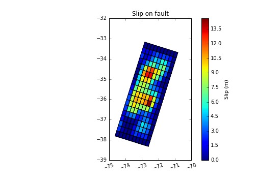
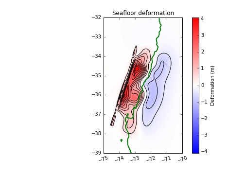
Computer simulation of tsunamis resulting from subduction zone earthquakes can be performed using a variety of available software packages, most of which implement the two-dimensional shallow water equations and require the vertical seafloor motion resulting from the earthquake as the input to initiate the waves. For recent past events this can be approximated based on source inversions; one example is shown in Figure 1. However, there are several situations in which it is desirable to instead generate hypothetical future earthquakes. In particular, recent work on probabilistic tsunami hazard assessment (PTHA) has focused on producing maps that indicate the annual probability of flooding exceeding various depths and can provide much more information than a single “worst considered case” inundation map (for example Adams et al (2015); Geist and Parsons (2006); Geist et al (2009); González et al (2009); Jaimes et al (2016); Løvholt et al (2012); Witter et al (2013)). This requires running tsunami simulations for many potential earthquakes and combining the results based on the annual probability of each, or using a Monte Carlo approach to sample a presumed probability density of potential earthquakes. Generating a large number of hypothetical events can also be useful for testing inversion methods that incorporate tsunami data, such as the current DART buoy network, or that might give early tsunami warnings for the nearshore (e.g., Melgar et al (2016)). Both Probabilistic Seismic Hazard Assessment (PSHA) and PTHA are also fundamental tools in the development of building codes that are critical in the design of structures able to withstand seismic and tsunami forces (e.g., Chock (2015)).

Figure 1: An example of slip distributed on a fault plane, from the USGS inversion of the 27 February 2010 event off Maule, Chile USGS (2010). The plot on the right shows the resulting sea floor deformation computed using the Okada model, with the coast line in green.

The primary goal of this paper is to introduce a general approach to generating hypothetical earthquakes, by producing random slip patterns on a pre-specified fault geometry. Similar techniques have been used in past studies, particularly for the generation of seismic waves in PSHA, which has a longer history than PTHA. A variety of techniques have been proposed for generating random seismic waveforms, see for example Anderson (2015); Dreger et al (2015); Frankel (1991); Ghofrani et al (2013); Guatteri et al (2003); Lavallée et al (2006); Motazedian and Atkinson (2005); Mai and Beroza (2002). One approach is to use a spectral representation of the slip pattern as a Fourier series with random coefficients that decay at a specified rate based on the desired smoothness and correlation length of the slip patterns, e.g as estimated from past events in the work of Mai and Beroza (2002). A random Fourier series can also be trimmed down to the desired non-rectangular fault geometry, possibly with some tapering to zero slip at some edges of the fault. Different correlation lengths can be specified in the strike and slip directions, if these directions are used as the horizontal coordinates in the Fourier representation and the fault is roughly rectangular.

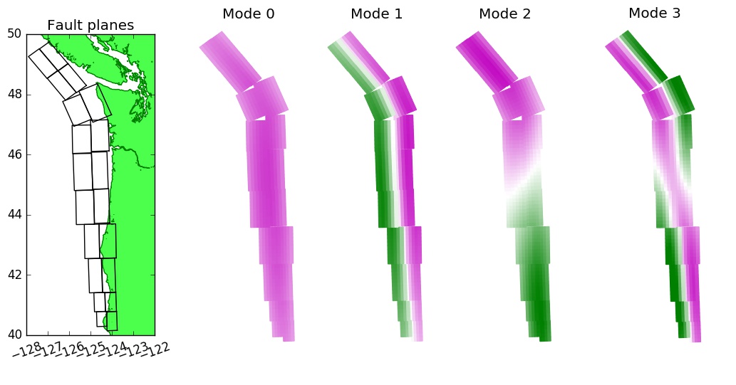
Our approach is essentially the same on a rectangular fault but generalizes easily to other fault geometries by using a Karhunen-Loève expansion. This work was motivated in particular by the need to model events on the curving Cascadia Subduction Zone (CSZ), which lies offshore North America and runs nearly 1200 km from Northern California up to British Columbia, see Figure 2.

Figure 2: Subdivision of the Cascadia Subduction Zone into 20 subfaults. These are further divided into 865 subfaults to compute the modes shown, which are the first four eigenvectors of the $865\times 865$ covariance matrix as might be used in a Karhunen-Lòeve expansion. Magenta and green are used to indicate positive and negative entries in the eigenmodes.

The fault is subdivided into many rectangular subfaults and a value of the slip $s_{i}$ is assigned to the $i$th subfault. If here are $N$ subfaults, then this defines a vector ${\bm{s}}\in{{\rm l}\kern-1.49994pt{\rm R}}^{N}$. Initially we assume that the moment magnitude $M_{w}$ of the earthquake (which depends on the total slip summed over all subfaults) has been prescribed, and also that the desired mean slip ${\bm{\mu}}\in{{\rm l}\kern-1.49994pt{\rm R}}^{N}$ and covariance matrix $\hat{\bm{C}}\in{{\rm l}\kern-1.49994pt{\rm R}}^{N\times N}$ are known. The mean slip is a vector with components $\mu_{i}=E[s_{i}]$, the expected value of the slip on the $i$th subfault, and the $N\times N$ covariance matrix $\hat{\bm{C}}$ has components $\hat{C}_{ij}=E[(s_{i}-\mu_{i})(s_{j}-\mu_{j})]$, which can also be expressed as the outer product $\hat{\bm{C}}=E[({\bm{s}}-{\bm{\mu}})({\bm{s}}-{\bm{\mu}})^{T}]$, where $T$ denotes transposing the vector.

The Karhunen-Loève (K-L) expansion (e.g. Ghanem and Spanos (1991); Huang et al (2001); Karhunen (1947); Loève (1977); Schwab and Todor (2006)) is a standard approach to representing a random field as a linear combination of eigenvectors of the presumed covariance matrix $\hat{\bm{C}}$. If the matrix $\hat{\bm{C}}$ has eigenvalues $\lambda_{k}$ (ordered with $\lambda_{0}>\lambda_{1}>\cdots>0$) and corresponding eigenvectors ${\bm{v}}_{k}$, then the K-L expansion expresses the slip vector ${\bm{s}}$ as

$${\bm{s}}={\bm{\mu}}+\sum_{k=1}^{N}z_{k}\sqrt{\lambda_{k}}{\bm{v}}_{k}.$$ (1)

where the $z_{k}$ are independent normally distributed random numbers $z_{k}\sim{\cal N}(0,1)$ with mean 0 and standard deviation 1. This is described in more detail in Section 2 where we explain why this gives random slip patterns with the desired mean and covariance. This expansion makes it easy to generate an arbitrary number of realizations using standard software to generate ${\cal N}(0,1)$ random numbers.

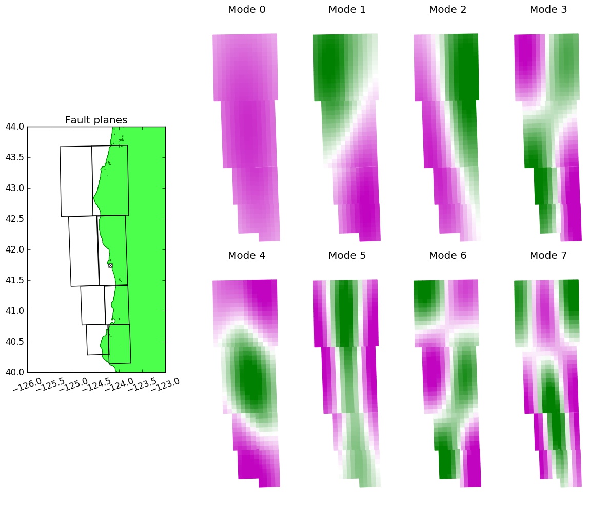
Figure 2 shows an example of the first four eigenmodes for the CSZ using this approach, where the $N$ components of each eigenvector are represented on the fault geometry using a color map in which magenta is positive and green is negative. Note that Mode 0 is roughly constant over the fault, so adding a multiple of this mode modifies the total slip and hence the magnitude $M_{w}$. On the other hand the other modes have both positive and negative regions and so adding a multiple of any of these tends to redistribute the slip (e.g., up-dip / down-dip with Mode 1 or between north and south with Mode 2). As with Fourier series, higher order eigenmodes are more oscillatory.

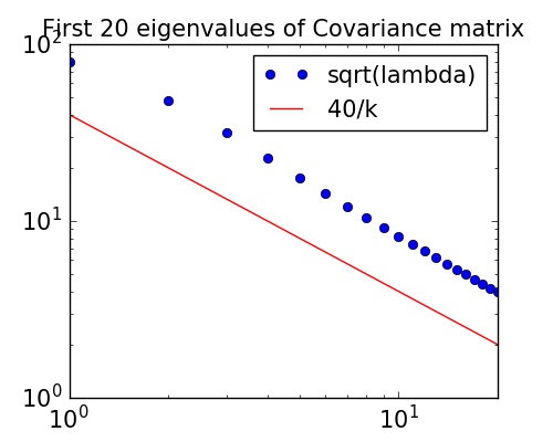
If the presumed correlation lengths are long and the covariance is a sufficiently smooth function of the distance between subfaults, then the eigenvalues $\lambda_{k}$ decay rapidly (there is little high-frequency content) and so the K-L series can often be truncated to only a few terms, greatly reducing the dimension of the stochastic space that must be explored.

The K-L series approach could also be used to generate random slip patterns for generating seismic waves, e.g. for performing PSHA or testing seismic inversion algorithms. In this case high-frequency components of the slip are very important and the K-L expansion may not decay so quickly. However, for tsunami modeling applications the slip pattern on the fault is only used to generate the resulting seafloor deformation. This is a smoothing operation that suppresses high frequencies. In this paper we also explore this effect and show that truncating the expansion to only a few terms may be sufficient for many tsunami applications. Reducing the dimension of the stochastic space is important for efficient application of many sampling techniques that could be used for PTHA analysis.

In this paper we focus on explaining the key ideas in the context of a one-dimensional fault model (with variation in slip only in the down-dip direction) and a two-dimensional example using the southern portion of the CSZ. However, we do not claim to have used the optimal parameters for modeling this particular fault. We also do not fully explore PTHA applications here, and for illustration we use some quantities of interest related to a tsunami that are easy to compute from a given slip realization, rather than performing a full tsunami simulation for each. This allows us to explore the statistics obtained from a large number of realizations (20,000) in order to illustrate some possible applications of this approach and explore the effects of truncating the K-L series. Work is underway to model the CSZ in a realistic manner and couple this approach with a full tsunami model.

The K-L expansion as described above generates a Gaussian random field, in which each subfault slip $s_{i}$ has a normal distribution with mean $\mu_{i}$ and variance $\hat{C}_{ii}$ and together they have a joint normal distribution with mean ${\bm{\mu}}$ and covariance matrix $\hat{\bm{C}}$. A potential problem with this representation is that when the variance is large it is possible for the slip $s_{i}$ to be negative on some subfaults. Since we assume the rake is constant (e.g. 90 degrees for a subduction thrust event), this would correspond to subfaults that are slipping in the wrong direction. The same issue arises with Fourier series representations and can be dealt with by various means, for example by simply setting the slip to zero any place it is negative (and then rescaling to maintain the desired magnitude). This naturally changes the statistics of the resulting distributions.

Another approach is to instead posit that the random slip can be modeled by a joint lognormal distribution, for which the probability of negative values is zero. Random slip patterns with a joint lognormal distribution can be generated by using the K-L expansion to first compute a Gaussian field and then exponentiating each component of the resulting vector to obtain the slip on each subfault. By choosing the mean ${\bm{\mu}}^{g}$ and covariance matrix $\hat{\bm{C}}^{g}$ for the Gaussian field properly, the resulting lognormal will have the desired mean ${\bm{\mu}}$ and $\hat{\bm{C}}$ for the slip. This is discussed in Section 4 and used in the two-dimensional example in Section 5.

2 Expressing slip using a Karhunen-Loève expansion

If the earthquake fault is subdivided into $N$ small rectangular subfaults, then a particular earthquake realization can be described by specifying the slip on each subfault, i.e. by a vector ${\bm{s}}\in{{\rm l}\kern-1.49994pt{\rm R}}^{N}$ where $s_{i}$ is the slip on the $i$th subfault. Note that we are assuming that only the slip varies from one realization to another; the geometry and rake (direction of slip on each subfault) are fixed, and the slip is instantaneous and not time-dependent. These restrictions could be relaxed at the expense of additional dimensions in our space of realizations.

Initially assume we wish to specify that the slip is a Gaussian random field with desired mean slip ${\bm{\mu}}\in{{\rm l}\kern-1.49994pt{\rm R}}^{N}$ and covariance matrix $\hat{\bm{C}}\in{{\rm l}\kern-1.49994pt{\rm R}}^{N\times N}$, which we write as ${\bm{s}}\sim{\cal N}({\bm{\mu}},\hat{\bm{C}})$. Then we compute the eigenvalues $\lambda_{k}$ of $\hat{\bm{C}}$ and corresponding normalized eigenvectors ${\bm{v}}_{k}$ so that the matrix of eigenvectors ${\bm{V}}$ (with $k$th column ${\bm{v}}_{k}$) and diagonal matrix of eigenvalues ${\bm{\Lambda}}$ satisfy $\hat{\bm{C}}={\bm{V}}{\bm{\Lambda}}{\bm{V}}^{T}$. Note that the covariance matrix is symmetric postive definite, so the eigenvalues are always positive real numbers and the eigenvectors can be chosen to be orthonormal, ${\bm{V}}^{-1}={\bm{V}}^{T}$.

Then the K-L expansion (1) can be written in matrix-vector form as

$${\bm{s}}={\bm{\mu}}+{\bm{V}}{\bm{\Lambda}}^{1/2}{\bm{z}},$$ (2)

where ${\bm{z}}\in{{\rm l}\kern-1.49994pt{\rm R}}^{N}$ is a vector of independent identically distributed ${\cal N}(0,1)$ random numbers. Realizations generated via the K-L expansion have the right statistics since we can easily compute that $E[{\bm{s}}]={\bm{\mu}}$ (since $E[{\bm{z}}]={\bm{0}}$) and

$$\begin{split}E[({\bm{s}}-{\bm{\mu}})({\bm{s}}-{\bm{\mu}})^{T}]&=E[{\bm{V}}{\bm{\Lambda}}^{1/2}{\bm{z}}{\bm{z}}^{T}{\bm{\Lambda}}^{1/2}{\bm{V}}^{T}]\\ &={\bm{V}}{\bm{\Lambda}}^{1/2}E[{\bm{z}}{\bm{z}}^{T}]{\bm{\Lambda}}^{1/2}{\bm{V}}^{T}\\ &={\bm{V}}{\bm{\Lambda}}{\bm{V}}^{T}=\hat{\bm{C}}\end{split}$$ (3)

using the fact that ${\bm{V}}$ and ${\bm{\Lambda}}$ are fixed and $E[{\bm{z}}{\bm{z}}^{T}]={\bm{I}}$. Note that the ${\bm{z}}$ could be chosen from a different probability density with mean ${\bm{0}}$ and covariance matrix ${\bm{I}}$ and achieve the same covariance matrix $\hat{\bm{C}}$ with the K-L expansion, although the ${\bm{s}}$ would not have a joint normal distribution in this case.

3 One-dimensional case: down-dip variation

We first illustrate this technique on a simplified case, a rectangular fault plane that is essentially infinitely long in the strike direction and with uniform slip in that direction, similar to the test case used by Løvholt et al (2012). The slip will only vary in the down-dip direction, reducing the problem to a single space dimension. The fault width is 100 km, a typical width for subduction zone faults, and is assumed to dip at $13^{\circ}$ from horizontal, with the upper edge at a depth of 5 km below the sea floor.

For the tests we perform here, we will focus on events of a single specified magnitude. The moment magnitude $M_{w}$ is a function of the total slip integrated over the entire fault plane, and also depends on the rigidity of the rock. For typical rigidity parameters, an average of 10 m of slip distributed over a fault that is 100 km wide and 1000 km long would result in a magnitude $M_{w}\approx 9.0$ and so we fix the total slip to have this average. If the fault were only half as long, 500 km, then this would be a $M_{w}\approx 8.8$ event and 20 m average slip would be required for a magnitude 9 event. With the exception of the potential energy shown in Figure 7, the quantities of interest considered in this paper are all linear in the total slip, however, so it does not really matter what value we choose.

An important aspect of PTHA analysis is to consider possible events of differing magnitudes as well, and take into account their relative probabilities. For smaller earthquakes, the Gutenberg-Ricter relation approximately describes their relative frequency, but for large subduction zone events that may have a recurrence time of hundreds of years, there is generally no simple model for the variation of annual probability with magnitude. There may be a continuous distribution of magnitudes or there may be certain “characteristic earthquakes” that happen repeatedly after sufficient stress has built up. The lack of detailed data for past events over a long time period makes this difficult to assess.

For the purposes of this paper, we assume that an earthquake of a particular magnitude occurs and we wish to model the range of possible tsunamis that can arise from such an event. We thus discuss the relative probability of different slip patterns and tsunamis given that an event of this magnitude occurs, and so the probability density should integrate to 1. This could then be used as one component in a full PTHA analysis by weighting these results by the probability that an event of this magnitude occurs and combining with similar results for other magnitudes. Alternatively, one could introduce the magnitude as an additional stochastic dimension and assume some probability density function for this, as we also discuss further below.

We use $x$ to denote the distance down-dip and split the fault into $N$ segments of equal width $\Delta x$, where $N\Delta x$ is the total width of the fault in the dip direction. We then specify $N$ slips $s_{i}$ for $i=1,~{}2,~{}\ldots,~{}N$. In our one-dimensional experiments we take $N=200$. This is finer than one would use in two dimensions and much finer than is needed to represent slip at an adequate level for either seismic or tsunami modeling. (For example, note from Figure 1 that the seismic inversion for this event represents the slip as piecewise constant on a $18\times 10$ grid with only 10 segments in the down-dip direction.) One could certainly reduce the dimension of the stochastic space below $N=200$ by using fewer subfaults. However, we will show that the dimension can be drastically reduced by instead using the K-L expansion reduced to only a few terms (e.g. 3, for this one-dimensional model the parameter choices below). By starting with a fine discretization of the fault, the eigenmodes used are smooth and perhaps better represent actual slip patterns than piecewise constant functions over large subfaults.

We assume that the $N$ slips are to be chosen randomly from a joint normal distribution with mean ${\bm{\mu}}=[\mu_{1},~{}\mu_{2},~{}\ldots,~{}\mu_{N}]^{T}$. The mean is chosen to be the desired taper, scaled to have the desired total slip. As an illustration of taper we use the function

$$\tau(d)=1-\exp(-20(d-d_{max})/d_{max})$$ (4)

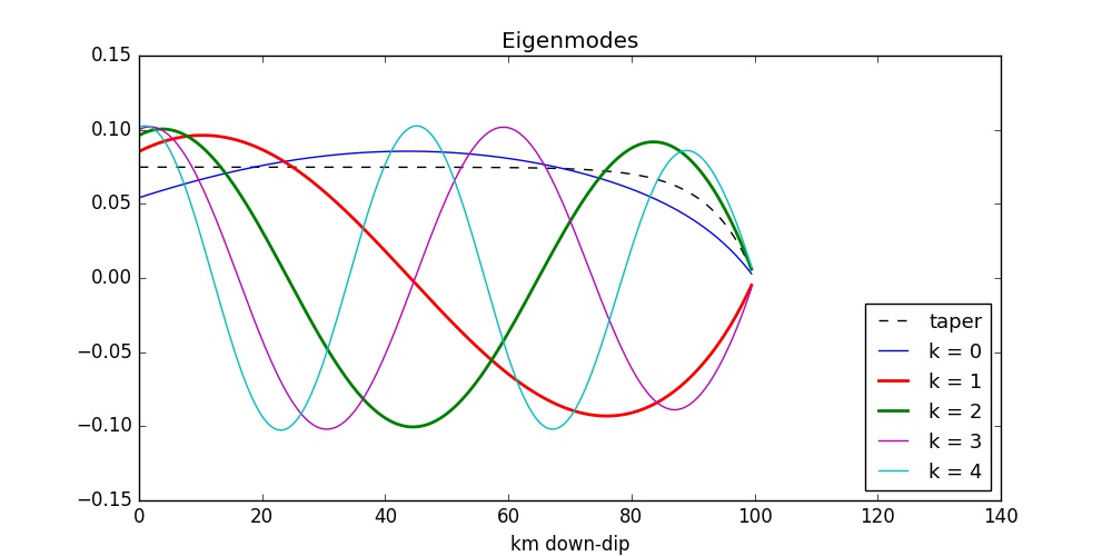
where $d$ is the depth of a subfault and $d_{max}=22500$m is the maximum depth of the fault. This function is close to 1 over most of the fault but tapers toward the down-dip edge. This taper, after scaling to give the mean slip, is shown as the dashed line in Figure 3. Other tapers can be used instead, e.g. the taper propsed by Wang and He (2008).

Figure 3: Eigenvalues decay like $1/k^{2}$ when the exponential autocorrelation function is used. The corresponding eigenvectors are similar to Fourier modes, shaped by the taper.

We set the desired covariance matrix to be $\hat{C}_{ij}=\sigma_{i}\sigma_{j}C_{ij}$ where $\sigma_{i}=\alpha\mu_{i}$ for some scalar $\alpha\in{{\rm l}\kern-1.49994pt{\rm R}}$ and ${\bm{C}}$ is the desired correlation matrix. We take $\alpha=0.75$, which tends to keep the slip positive everywhere, as desired, while still giving reasonable variation in slip patterns. The correlation matix is given by $C_{ij}={\tt corr}(|x_{i}-x_{j}|)$ in terms of some autocorrelation function (ACF) ${\tt corr}(r)$, and we choose

$${\tt corr}(r)=\exp(-r/r_{0}),$$ (5)

where the correlation length is set to $r_{0}=0.4W=40$ km, i.e., 40% of the fault width as suggested by Mai and Beroza (2002).

Figure 3 shows the taper along with the first several eigenvectors of the covariance matrix ${\bm{C}}$ (ordered based on the magnitude of the eigenvalues, with eigenvectors normalized to have vector 2-norm equal to 1). Note that the lowest mode 0 looks very similar to the taper. Adding in a multiple of this mode will modify the total slip and hence the magnitude, so we drop this mode from the sum. The higher modes are orthogonal to mode 0 and hence do not tend to change the total slip. They look like Fourier modes that have been damped near the down-dip boundary by the taper.

To create a random realization, we choose a vector ${\bm{z}}$ of $N$ i.i.d. Gaussian ${\cal N}(0,1)$ values $z_{k}$ for $k=0,~{}1,~{}\ldots,~{}N-1$. If we neglect the 0-mode and truncate the expansion after $m$ terms, then this amounts to setting $z_{0}=0$ and $z_{k}=0$ for $k>m$. We will denote such a ${\bm{z}}$ vector by ${\bm{z}}^{[m]}$. The slip pattern can then be written as

$${\bm{s}}={\bm{\mu}}+{\bm{V}}{\bm{\Lambda}}^{1/2}{\bm{z}}^{[m]}.$$ (6)

The left column of Figure 4 shows the mean slip in the top plot, followed by several random realizations generated by the K-L expansion using 20 terms, with the ${\bm{z}}^{[20]}$ coefficients chosen as i.i.d. ${\cal N}(0,1)$ values. These are the blue curves in each plot. In each case, the slip is also shown when only 3 terms in the series are used (i.e. ${\bm{z}}^{[3]}$ is computed by leaving $z_{1},~{}z_{2},~{}z_{3}$ unchanged from ${\bm{z}}^{[20]}$ but with the higher terms dropped, equivalent to truncating the expansion at an earlier point). These slip patterns, shown in red, are smoothed versions of the 20-term slip patterns since the higher wave number components have been surpressed. In many cases there appears to be quite a large difference between the 3-term and 20-term slips. This is a reflection of the fact that the eigenvalues do not decay all that quickly in this case. There would be faster decay if a longer correlation length were chosen, and much more rapidly if the Gaussian autocorrelation function were chosen instead of the exponential.

Figure 4: The left column shows slip on the fault plane of width $W=100$ km. The right column shows the resulting seafloor deformation if the up-dip edge of the fault plane is 5 km below the surface and it dips at $13^{\circ}$. The top row shows the mean slip and resulting deformation. The remaining rows show random realizations using 20 terms of a K-L expansion (blue) and the same sum truncated to 3 terms (red).

In spite of the differences in the slip patterns, for tsunami modeling the 3-term series may still be adequate. The right column of Figure 4 shows the sea floor deformations that result from the slips shown on the left. The blue curves show the deformation due to the 20-term sum while the red curves show the deformation resulting from the truncated 3-term sum. As mentioned earlier, high wavenumber oscillations in the slip pattern are filtered out by the Okada model used to compute the seafloor deformation $\Delta\bm{B}$ from the slip ${\bm{s}}$. If the $\Delta\bm{B}$ are sufficiently similar between the 3-term and the full K-L expansion, then there is no reason to use more terms. In this case we have reduced the stochastic space that needs to be explored down to 3 dimensions. There is much greater similarity for some realizations than for others, and so below we examine the statistical properties of this approximation by using a sample of 20,000 realizations.

Note that using only 3 modes may be too few for this particular set of fault parameters — the comparisons shown in Figure 4 would look more similar if a few more terms were retained — but we will see that good statistical properties are obtained even with this severe truncation. How many terms are required depends on various factors: not only the correlation structure of the slip as discussed above, but also the depth of the fault plane. The deeper it is, the more smoothing takes place in the Okada model. Here we placed the top of the fault plane at 5 km depth. This is a typical depth but there is variation between subduction zones.

To examine statistical properties of the 20-term sum and the 3-term approximation, we generate 20,000 samples of each and compare some quantities that are cheap to compute but that are important indicators of the severity of the resulting tsunami. Running a full tsunami model based on the shallow water equations is not feasible for this large number of realizations, but the quantities we consider will stand in as proxies for the quantities one might actually want to compute, such as the maximum depth of flooding at particular points onshore. Moreover the distribution of these proxy values can be used in a later stage to help choose particular earthquake realizations for which the full tsunami model will be run. It is desirable to run the model with judiciously chosen realizations for which the proxy values are well distributed over the range of possible values. The computed densities of the proxy values can also be used to weight the results from the full model runs to accurately reflect the probabities of such events. This will be explored in detail in a future paper.

Computations for a large number of realizations can be sped up substantially by realizing that the Okada model is linear in the slip, i.e. if the slip vector is given by ${\bm{s}}$ then the resulting sea floor deformation can be written as $\Delta\bm{B}={\bm{\Theta}}{\bm{s}}$ for a matrix ${\bm{\Theta}}\in{{\rm l}\kern-1.49994pt{\rm R}}^{N_{B}\times N}$, where $N_{B}$ is the number of grid points where the deformation $\Delta\bm{B}$ is computed (in our experiments we use $N_{B}=1001$ over an interval that extends 100 km on either side of the fault region). The Okada model implemented in the GeoClaw dtopotools Python module is used, which directly computes $\Delta\bm{B}$ from ${\bm{s}}$ and so we do not actually compute the matrix ${\bm{\Theta}}$, but it is useful conceptually. In particular, if the K-L expansion (6) is to be used to compute ${\bm{s}}$ then we find that

$$\Delta\bm{B}={\bm{\Theta}}{\bm{\mu}}+{\bm{\Theta}}{\bm{V}}{\bm{\Lambda}}^{1/2}{\bm{z}}^{[m]}.$$ (7)

The vector ${\bm{\Theta}}{\bm{\mu}}$ is obtained by applying Okada to the mean slip vector. The matrix ${\bm{\Theta}}{\bm{V}}$ can be computed by applying Okada to each column of ${\bm{V}}$ to compute the columns of the product matrix. Since the sum only involves $m$ nonzero terms, we need only apply Okada to columns 1 through $m$ of ${\bm{V}}$ (i.e. the first $m$ K-L modes ${\bm{v}}_{1},~{}{\bm{v}}_{2},~{}\ldots,~{}{\bm{v}}_{m}$ used to express $s$). Hence if we plan to use at most 20 modes of the K-L expansion then we need only apply the Okada model to 21 slip vectors and we can then take linear combinations of the resulting sea floor deformations, rather than applying Okada to 20,000 slip realizations separately.

In practice this can be simplified further. Applying Okada to a mode ${\bm{v}}_{k}$ actually requires applying Okada to each of the $N$ subfaults, weighting by the corresponding element of ${\bm{v}}_{k}$, and summing over all the subfaults. So applying Okada to $m$ modes in this way actually requires applying Okada $mN$ times. Instead, we can first apply the Okada model to $N$ unit source scenarios in which the slip is set to 1 on the $j$th subfault and to 0 on all other subfaults. Call this slip vector ${\bm{s}}^{[j]}$. Applying Okada to this gives a resulting $\Delta\bm{B}^{[j]}={\bm{\Theta}}{\bm{s}}^{[j]}$. Now for any slip vector ${\bm{s}}$ we can compute ${\bm{\Theta}}{\bm{s}}$ as

$${\bm{\Theta}}{\bm{s}}=\sum_{j=1}^{N}s_{j}\Delta\bm{B}^{[j]}.$$ (8)

In particular taking ${\bm{s}}={\bm{v}}_{k}$ would give ${\bm{\Theta}}{\bm{v}}_{k}$, but (8) can be used directly to compute the seafloor deformation $\Delta\bm{B}={\bm{\Theta}}{\bm{s}}$ for any slip realization. This approach can also be used in the lognormal case described in Section 4 and employed in Section 5.

Subsidence or uplift. One quantity that has a significant impact on the severity of tsunami flooding is the vertical displacement of the seafloor at the coast. If this displacement is negative and the land subsides at the shore, then flooding will generally be much worse than if uplift occurs. The behavior seen for a particular event depends on how far offshore the subduction zone is, which is generally directly related to the width of the continental shelf offshore from the community of interest (since the top edge of the fault is usually located near the trench at the edge of the shelf, which is part of the continental plate beneath which the oceanic plate is subducting). This distance can vary from only a few km (e.g. along the Mexico coast) to 200 km (e.g. along the coast of Japan where the Tohoku event occurred). In our model the top of the plate is at $x=0$ and we choose the coast line location to be at $x=75$ km, which gives a wide range of subsidence and uplift values, as can be observed for the realizations shown in Figure 4.

The displacement at one particular point is easy to determine from each realization, it is just one entry in the vector of sea floor deformation obtained from the Okada model, say $\Delta\bm{B}_{j}={\bm{e}}_{j}^{T}\Delta\bm{B}$ for some $j$, where ${\bm{e}}_{j}$ is the unit vector with a 1 in position $j$. (We have evaluated $\Delta\bm{B}$ on a fine grid so we assume we don’t need to interpolate). As such, this particular quantity is in fact easy to compute directly from ${\bm{z}}$ for any given realization, as

$$\Delta B_{\scriptstyle{shore}}=\Delta B_{\scriptstyle{shore}}(\mu)+{\bm{b}}^{T}{\bm{z}},$$ (9)

where $\Delta B_{\scriptstyle{shore}}(\mu)={\bm{e}}_{j}^{T}{\bm{\Theta}}{\bm{\mu}}$ is the shoreline displacement resulting from the mean slip and the row vector ${\bm{b}}^{T}$ is

$${\bm{b}}^{T}={\bm{e}}_{j}^{T}{\bm{\Theta}}{\bm{V}}{\bm{\Lambda}}^{1/2},$$ (10)

i.e. the vector consisting of the $j$th component of the sea floor displacement resulting from applying Okada to each K-L mode, scaled by the square root of the corresponding eigenvalue. From (9) it follows immediately that $\Delta B_{\scriptstyle{shore}}$ is normally distributed with mean $\Delta B_{\scriptstyle{shore}}(\mu)$ and variance $\sigma^{2}=\sum_{k=1}^{m}b_{k}^{2}$ (in the Gaussian case considered here, not in the lognormal case considered below). Hence for this particular quantity of interest in the Gaussian case, we do not need to estimate the statistics based on a large number of samples. We can immediately plot the Gaussian density function for the “full” expansion with 20 terms and compare it to the density for the truncated series with only 3 terms. These are seen to lie nearly on top of one another in Figure 5. This plot also shows the density that would be obtained with only 1 or 2 terms in the K-L expansion, which are substantially different. This confirms that, in terms of this particular quantity of interest, it is sufficient to use a 3-term K-L expansion (but not fewer terms).

Figure 5: The figure on the left shows the true Gaussian density for the shoreline displacement for K-L expansions with 1, 2, 3, or 20 terms. The figure on the right shows the kernel density estimate from 20,000 samples using 3 terms or 20 terms, together with the true density for 20 terms.

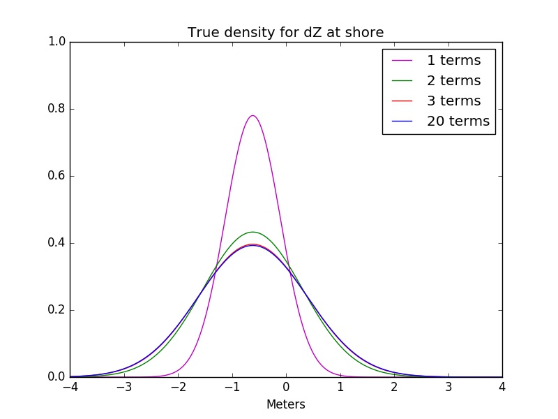
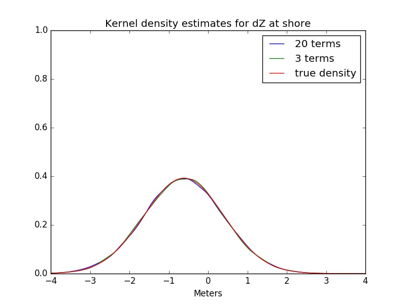
Figure 5 also shows the density as estimated using 20,000 samples, using a kernel density estimate computed using the Python package seaborn of Waskom (2015). With either 3 terms or 20 terms, the estimated density lies nearly on top of the true density, giving confidence that the sampling has been programmed properly and that 20,000 samples is sufficient since the true density is known in this case.

Potential energy. From the samples it is possible to also estimate the densities for other quantities of interest for which it is not possible to compute the true density. We consider two additional quantities that have relevance to the magnitude of the tsunami generated. One is the potential energy of the initial perturbation of the ocean surface, which is one measure of its potential for destruction. The potential energy is given by

$$E=\frac{1}{2}\int\int\rho g\eta^{2}(x,y)\,dx\,dy$$ (11)

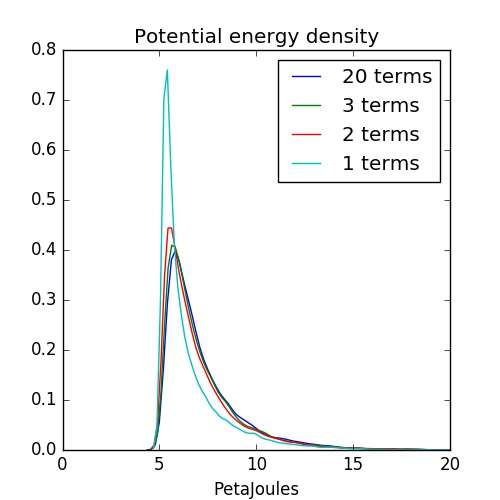
where $\rho=1000$ kg/m³ is the density of water, $g=9.81$ m/s², and $\eta(x,y)$ is the initial perturbation of the surface. With our assumption that the sea surface moves instantaneously with sea floor deformation generated from the slip, $\eta$ is equal to the sea floor displacement in the ocean, while onshore we set $\eta=0$ since displacement at these points does not contribute to the potential energy of the tsunami. For the one-dimensional problem considered here, we sum the square of the displacement over $x<75$ km and scale by $\rho gL\Delta x$ to define $E$, taking $L=100$ km. Finally we multiply by $10^{-15}$ so that the results are order 1, with units of PetaJoules. We use the kernel density estimator of seaborn to plot the results obtained with 20,000 samples, using 20 terms or truncating further to 1, 2, or 3 terms. The results in Figure 6 again show that 3 terms is sufficient to obtain very similar results to 20 terms.

Figure 6: Kernel density estimates based on 20,000 samples, using 1, 2, 3, or 20 terms in the K-L expansion. The left figure shows the potential energy (11) and the right figure shows the maximum amplitude of deformation (sea surface elevation).

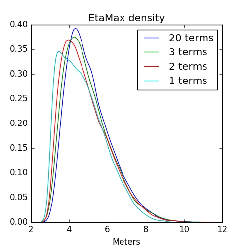
Maximum wave height. The maximum positive seafloor displacement gives the maximum amplitude of the tsunami at the initial time. We expect this to be positively correlated with the amplitude of the wave that approaches shore (although the wave propagation can be complicated by multiple peaks, the location of the $\eta_{max}$ relative to the shore, or various other factors that can only be studied with a full tsunami model). The right plot of Figure 6 shows the kernel density estimates of this quantity $\eta_{max}$.

Joint probability densities. It is also interesting to plot the joint probability density of pairs of quantities to better explore the ability of 3 terms to capture the variation. This is illustrated in Figure 7, where the top row shows kernel density estimates (again computed using seaborn) for $E$ vs. $\eta_{max}$ and the bottom rows shows $\Delta B_{\scriptstyle{shore}}$ vs. $\eta_{max}$. In each case the left figure shows the density computed from 20,000 realizations of the 20-term K-L expansion while the right figure shows the density estimated from an equal number of 3-term expansions. In each case it appears that the 3-term expansion captures the bulk of the variation.

Figure 7: Joint and marginal probability densities for different quantities, comparing the densities estimated using the 20-term expansion (left column) and the 3-term expansion (right column). The top row shows the joint density of $\eta_{max}$ with potential energy $E$ of the tsunami generated. The bottom row shows the joint density of $\eta_{max}$ with $\Delta B_{\scriptstyle{shore}}$, the vertical displacement at the shore.

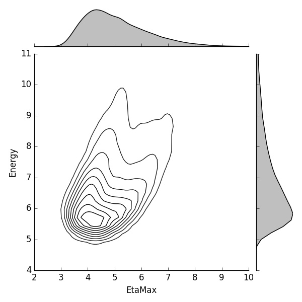
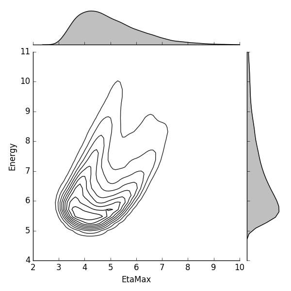
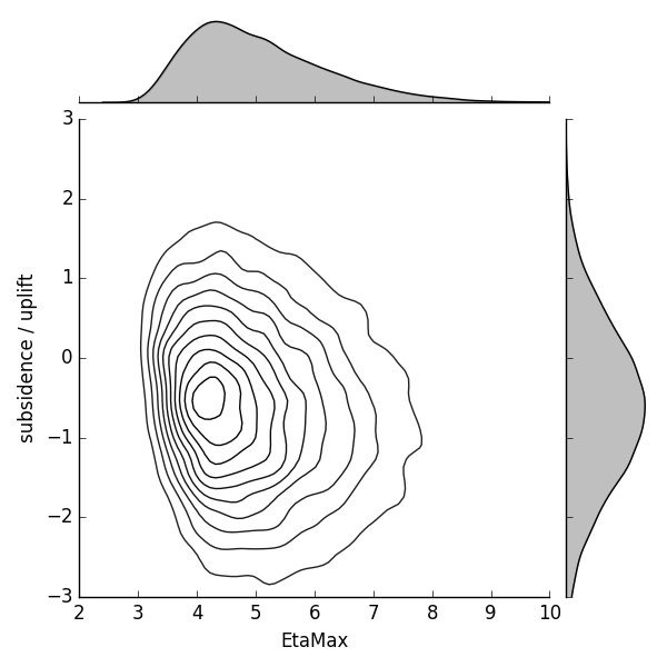
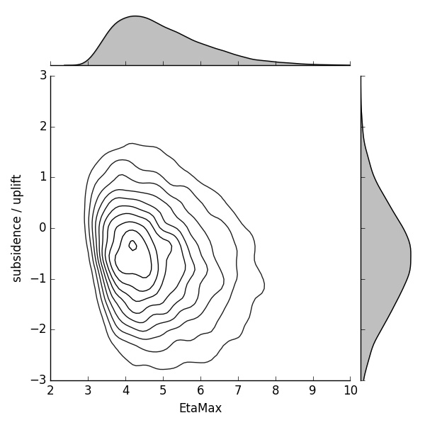
The joint distribution of $\eta_{max}$ and $\Delta B_{\scriptstyle{shore}}$ is of particular interest since the most dangerous events might be those for which $\eta_{max}$ is large while $\Delta B_{\scriptstyle{shore}}$ is most negative (greatest subsidence of the coast). The fact that the joint distributions look quite similar gives hope that the 3-term model will adequately capture this possibility.

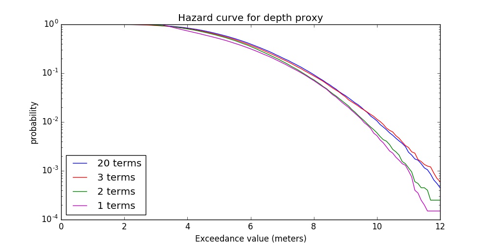
Depth proxy hazard curves. The goal of a full-scale PTHA exercise is often to generate hazard curves at many points onshore or in a harbor. A hazard curve shows, for example, the probability that the maximum flow depth will exceed some value as a function of that exceedance value. Construction of these curves is discussed, for example, in the appendices of González et al (2014). The curves may vary greatly with spatial location due to the elevation of the point relative to sea level, and also due to the manner in which a tsunami interacts with nearby topography. Hazard curves must thus be computed using fine-grid simulations of the tsunami dynamics and cannot be computed directly from the sea floor deformation alone. However, as a proxy for flooding depth we might use $D=\eta_{max}-\Delta B_{\scriptstyle{shore}}$, the maximum offshore sea surface elevation augmented by any subsidence that occurs at the shore. We do not claim that this is a good estimate of the actual maximum water depth that will be observed at the shore, but computing hazard curves for this quantity provides another test of how well the 3-term K-L expansion captures the full probability distribution described by the 20-term expansion. This curve is obtained by computing $D$ for each sample and determining the fraction of samples for which this is above $\zeta_{i}$, for each exceedance level $\zeta_{i}$ on a fine grid covering the range of $D$ observed. Figure 8 shows the resulting hazard curve obtained with the 20-term expansion. The curve obtained with the 3-term expansion is also shown, and lies nearly on top of it.

Figure 8: Hazard curves based on the proxy for flooding depth given by $\eta_{max}-\Delta B_{\scriptstyle{shore}}$. Based on 20,000 samples using the full 20-term K-L expansion, compared with the hazard curves obtained using only 1, 2, or 3 terms in the expansion. Note that 3 terms is sufficient to obtain the hazard curve to high precision.

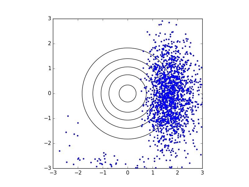
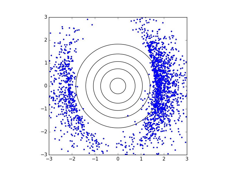
Exploring parameter space. One advantage of describing the probability space of possible events in terms of a small number of stochastic parameters is that it may be possible to examine structures in this space, which can be important in developing a cheap surrogate model to use in estimating probabilities and computing hazard curves for practical quantities of interest. For example, we can ask what parts of parameter space lead to the worst events. The left figure in Figure 9 shows the events (projected to the $z_{1}$-$z_{2}$ plane) from the above tests with the 3-term K-L expansion for which the proxy depth is greater than 8 m. The contours of the bivariate normal distribution are also plotted. A scatter plot of all 20,000 events would cluster in the middle, but we observe that the events giving this extreme depth tend to have $z_{1}>1$. From Figure 3 we see that positive $z_{1}$ redistributes slip from the down-dip to the up-dip portion of the fault. This agrees with common wisdom from past events that concentration near the up-dip edge gives particularly severe tsunamis (as in the case of the 2011 Tohoku event). The right figure in Figure 9 shows a similar scatter plot of $z_{1}$-$z_{2}$ values for which the potential energy was above 9.5 PetaJoules. In this case most of the extreme events have $z_{1}$ either very positive or very negative. In the latter case slip is concentrated toward the down-dip portion of the fault, which leads to a smaller maximum surface displacement but the displacement spreads out further spatially for a deep rupture which can lead to large potential energy since this is integrated over space.

Figure 9: Scatter plots in the $z_{1}$-$z_{2}$ plane of the subset of 3-term events for which the proxy depth is greater than 8 m (left) or for which the potential energy is greater than 9.5 PetaJoules (right).

4 Lognormally distributed slip

If we wish to instead generate slip realizations that have a joint lognormal distribution with a desired mean and covariance matrix, we can first generate realizations of a joint Gaussian random field and then exponentiate each component. This approach will be used in the two-dimensional example below in Section 5.

In this case we first choose the desired mean ${\bm{\mu}}$ and covariance matrix $\hat{\bm{C}}$ for the slip, and then compute the necessary mean ${\bm{\mu}}^{g}$ and covariance matrix $\hat{\bm{C}}^{g}$ for the Gaussian to be generated by the K-L expansion, using the fact that if ${\bm{g}}$ is a random variable from ${\cal N}({\bm{\mu}}^{g},\hat{\bm{C}}^{g})$, then $\exp({\bm{g}})$ is lognormal with mean and covariance matrix given by:

$$\mu_{i}=\exp(\mu_{i}^{g}+\hat{C}_{ii}^{g}/2),\qquad\hat{C}_{ij}=\mu_{i}\mu_{j}(\exp(\hat{C}_{ij}^{g})-1).$$ (12)

Hence we can solve for

$$\begin{split}\hat{C}_{ij}^{g}&=\log(\hat{C}_{ij}/\mu_{i}\mu_{j}+1),\\ \mu_{i}^{g}&=\log(\mu_{i})-\frac{1}{2}\hat{C}_{ii}^{g}.\end{split}$$ (13)

We now find the eigenvalues $\lambda_{k}$ and eigenvectors ${\bm{v}}_{k}$ of $\hat{\bm{C}}^{g}$. To generate a realization we choose $N$ values $z_{k}\sim{\cal N}(0,1)$ and then form the K-L sum

$${\bm{s}}^{g}={\bm{\mu}}^{g}+\sum_{k=0}^{N}z_{k}\sqrt{\lambda_{k}}{\bm{v}}_{k}.$$ (14)

We then exponentiate each component of ${\bm{s}}^{g}$ to obtain the slip values, which then have the desired joint lognormal distribution (see e.g., Ghanem (1999)).

As described, this will generate realizations with total slip (and hence magnitude $M_{w}$) that vary around the mean. As in the Gaussian case, we can drop the nearly-constant ${\bm{v}}_{0}$ term from the sum to reduce this variation. We can also generally truncate the series to a much smaller number of terms and still capture most of the variation if the eigenvalues are rapidly decaying.

Now consider the special case where we make the same assumptions as in Section 2 that $\hat{C}_{ij}=\sigma_{i}\sigma_{j}C_{ij}$ where ${\bm{C}}$ is the desired correlation matrix and $\sigma_{i}=\alpha\mu_{i}$, while the mean $\mu_{i}$ was given by some taper $\tau_{i}$ scaled by a scalar value $\bar{\mu}$. Then computing ${\bm{\mu}}^{g}$ and $\hat{\bm{C}}^{g}$ according to (13), we find that:

$$\begin{split}\hat{C}_{ij}^{g}&=\log(\alpha^{2}C_{ij}+1),\\ \mu_{i}^{g}&=\log(\bar{\mu}\tau_{i})-\frac{1}{2}\log(\alpha^{2}+1)\end{split}$$ (15)

We see that the covariance matrix in this case depends only on the correlation matrix and the scalar $\alpha$, not on the mean slip itself (and in particular is independent of the taper). We also find that $\exp(\mu_{i}^{g})=\bar{\mu}\tau_{i}/\sqrt{\alpha^{2}+1}$ is simply a scalar multiple of the taper.

Using these assumptions and the fact that

$$\exp\left({\bm{\mu}}^{g}+\sum_{k=1}^{N}z_{k}\sqrt{\lambda_{k}}{\bm{v}}_{k}\right)=\exp({\bm{\mu}}^{g})\exp\left(\sum_{k=1}^{N}z_{k}\sqrt{\lambda_{k}}{\bm{v}}_{k}\right),$$

it is easy to generate realizations that have exactly the desired magnitude: simply compute

$$\exp\left(\sum_{k=1}^{N}z_{k}\sqrt{\lambda_{k}}{\bm{v}}_{k}\right),$$ (16)

multiply the result by the desired taper, and then rescale by a multiplicative factor so that the area-weighted sum of the slips gives the total slip required for the desired seismic moment.

5 Two-dimensional case

We now present an example in which the slip is allowed to vary in both directions along a fault surface. For illustration we use a subset of the Cascadia Subduction Zone from Figure 2, taking only the southern-most 8 fault segments, as illustrated in Figure 10. These are subdivided into 540 smaller fault planes for the purposes of defining the slip.

To define the $540\times 540$ correlation matrix, we need to compute the pairwise “distance” between subfault $i$ and subfault $j$. We can compute the Euclidean distance $d_{ij}$, but for this fault geometry we expect a longer correlation length in the strike direction than down-dip, so we wish to define

$$C_{ij}=\exp(-(d_{\scriptstyle{strike}}(i,j)/r_{\scriptstyle{strike}})-(d_{\scriptstyle{dip}}(i,j)/r_{\scriptstyle{dip}}))$$ (17)

where $d_{\scriptstyle{strike}}(i,j)$ and $d_{\scriptstyle{dip}}(i,j)$ are estimates of the distance between subfaults $i$ and $j$ in the strike and dip direction, respectively, and $r_{\scriptstyle{strike}},r_{\scriptstyle{dip}}$ are the correlation lengths in each direction. We define $d_{\scriptstyle{dip}}(i,j)$ using the difference in depth between the two subfaults and the dip angle $\delta$ as $d_{\scriptstyle{dip}}(i,j)=d_{\scriptstyle{depth}}/\sin(\delta)$, setting $d_{\scriptstyle{strike}}(i,j)=\sqrt{d_{ij}^{2}-d_{\scriptstyle{dip}}(i,j)^{2}}$. We take the correlation lengths to be 40% of the fault length and width respectively, $r_{\scriptstyle{strike}}=130$km and $r_{\scriptstyle{dip}}=40$km. We again use an exponential autocorrelation function as defined in (17), but this could easily be replaced by a different ACF. We use the lognormal approach described in Section 4, with parameter $\alpha=0.5$. Figure 10 shows the first 8 eigenmodes of $\hat{\bm{C}}^{g}$. Again we drop Mode 0 from the sum, since this mode is roughly constant over the fault.

Figure 10: Southern portion of the CSZ fault showing location of Crescent City, CA and the 8 subfaults that are further subdivided into 540 subfaults. The first 7 eigenmodes of the resulting covariance matrix $\hat{\bm{C}}^{g}$ are also shown.

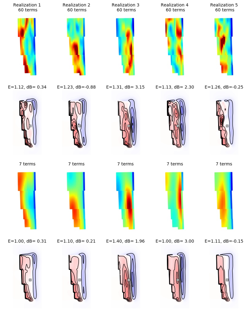
To create slip realizations, we use (16) and then apply a tapering only at the down-dip edge, given by (4) with $d_{max}=20000$m. We then scale the slip so that the resulting seismic moment gives $M_{w}=8.8$. Figure 11 shows 5 typical realizations, comparing the slip generated by a 60-term K-L expansion with the slip generated when the series is truncated after 7 terms. The resulting seafloor deformation in each case is also shown, along with the potential energy and the subsidence/uplift $\Delta B_{\scriptstyle{shore}}$ at one point on the coast, the location of Crescent City, CA. Note that in each case the 7-term series gives a smoother version of the slip obtained with 60 terms, and the seafloor deformations are more similar than the slip patterns, as expected from the one-dimensional analogous case shown in Figure 4. The potential energy and $\Delta B_{\scriptstyle{shore}}$ are also seen to be similar when the truncated series is used to the values obtained with the longer 60-term series.

Figure 11: The top row shows 5 sample realizations of slip on the southern CSZ fault, as computed with a 60-term K-L expansion. The second row shows the resulting seafloor deformation, with an indication of the potential energy and the vertical displacement at Crescent City, CA, which is indicated by the X in the figures. The third row shows the same 5 realizations but with the K-L series truncated to 7 terms, and the bottom row shows the resulting seafloor deformations.

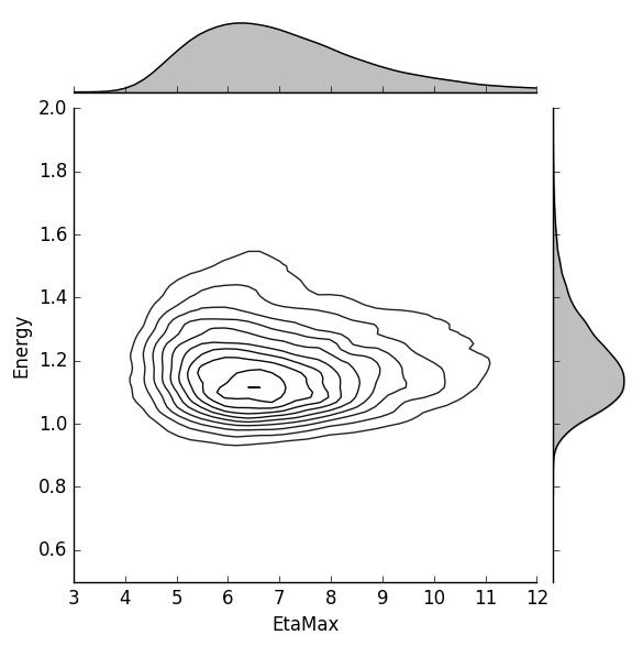
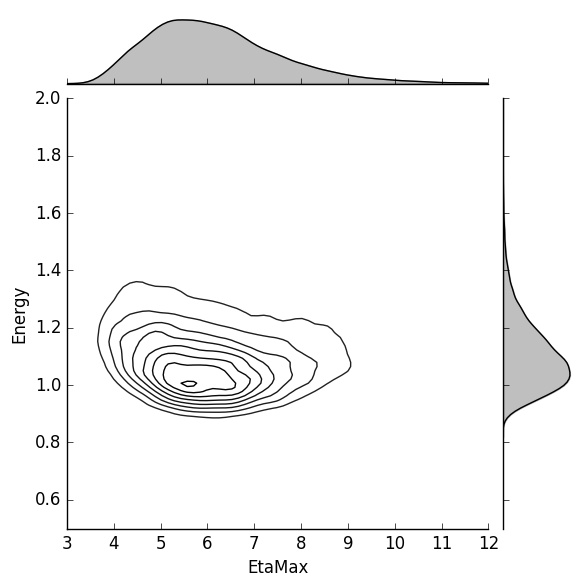
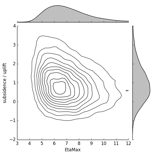
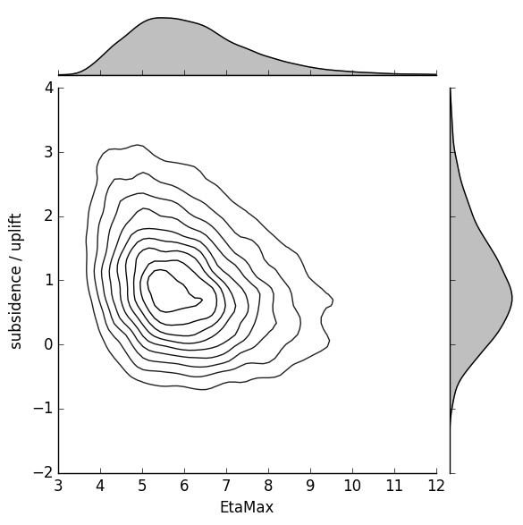
We can explore the statistical properties by repeating any of the experiments performed above in the one-dimensional case. In the interest of space, we only show one set of results, the same joint and marginal densities examined in the one-dimensional case in Figure 7. The comparisons for the two-dimensional fault are shown in Figure 12. To generate each column of figures we computed 20,000 slip realizations and the resulting seafloor deformations (via (8)). The first column shows statistics when a 60-term KL-expansions is used, producing realizations similar to those shown in the top row of Figure 11. The second column of figures was produced using an independent set of 7-term realizations (i.e. these were not obtained by truncating the 60-term series from the first set, but rather by generating 20,000 independent samples). Even in this two-dimensional case, less than 10 minutes of CPU time on a MacBook Pro laptop was required to generate each set of 20,000 realizations, the resulting seafloor deformations, and the kernel density plots.

Figure 12: Joint and marginal probability densities for different quantities, comparing the densities estimated using the 60-term expansion (left column) and the 7-term expansion (right column) for the two-dimensional fault case. The top row shows the joint density of $\eta_{max}$ with potential energy $E$ of the tsunami generated. The bottom row shows the joint density of $\eta_{max}$ with $\Delta B_{\scriptstyle{shore}}$, the vertical displacement at Crescent City, CA. In each case 20,000 realizations similar to those shown in Figure 11 were used to create these kernel density estimates.

6 Discussion

We have presented an approach to defining a probability distribution for earthquake slip patterns on a specified fault geometry that has been subdivided into an arbitrary number of rectangular subfaults, with a specified mean and covariance matrix. Slip realizations can be generated that either have a joint normal distribution or a joint lognormal distribution. Once the parameters have been chosen that define the distribution, it is very easy to generate an arbitrary number of sample realizations from the distribution, simply by drawing the coefficients $z_{k}$ of the K-L series from independent normal distributions.

We have also illustrated that with a realistic choice of correlation length, the K-L series can be truncated to a relatively small number of terms. For tsunami modeling applications, the Okada model is applied to each slip pattern to generate the seafloor deformation and it was shown that this is a smoothing operation that can further reduce the number of terms needed, and hence the dimension of the stochastic space that must be explored in doing PTHA analysis.

To use this approach for practical PTHA analysis, two major challenges must be addressed. The first is to tackle the epistemic uncertainty associated with the lack of knowledge about possible future earthquakes. We would like to choose the parameters defining the probability distribution in a suitable way for real fault geometries so that it accurately represents the space of possible future earthquakes. However, realistic specification of these critical seismic parameters and quantifying the associated uncertainties and geophysical contraints is a major challenge that Stein et al (2012) have reviewed and summarized; they characterize the problem as a failure of earthquake hazard mapping, in general, and make recommendations regarding improvements. The problem is particularly severe in the case of near-field PTHA studies, because tsunami impact on a coastal community is highly sensitive to details of the seismic deformation (e.g., Geist (2002)). Existing expertise and geophysical constraints should at least be incorporated in the choice of these parameters. The ability to generate many realizations and examine statistics of quantities such as those used in this paper may help in this. As one example, the parameters chosen in this paper for the CSZ example tend to give uplift rather than subsidence at Crescent City (as can be seen in the marginal distribution of subsidence/uplift in Figure 12). If this is viewed as inconsistent with the geological evidence from past events, this could be adjusted, for example by tapering the slip more on the down-dip side. Moving more of the slip up-dip will cause more subsidence at the shore. It would also be possible to explore ways in which the epistemic uncertainty associated with the lack of knowledge about the true probability distribution affect the resulting hazard maps generated by a PTHA analysis, for example by doing the analysis with different parameter choices, and hence different probability distributions, to see how robust the PTHA analysis is to changes in assumptions.

The second major challenge is to deal with the aleatoric uncertainty that is still present even if the parameters defining the probability distribution were known to be correct. We are still faced with a high-dimensional space to sample in order to perform PTHA analysis. For example, if we wish to compute a hazard curve similar to Figure 8 for the probability that the maximum depth $D$ at some particular point will exceed various depths, then for each exceedence value $D_{e}$ we need to calculate

$$P[D>D_{e}]=\int\rho({\bm{z}})I({\bm{z}};D_{e})\,d{\bm{z}}$$ (18)

where the integral is over the $m$-dimensional stochastic space of coefficients $z$ of the K-L sum (assuming $m$ terms are used) and $I({\bm{z}};D_{e})$ is an indicator function that is 1 at points ${\bm{z}}\in{{\rm l}\kern-1.49994pt{\rm R}}^{m}$ where the corresponding realization gives a tsunami that exceeds $D_{e}$ and 0 elsewhere (or it could take values between 0 and 1 to incorporate other uncertainties, e.g. if the approach of Adams et al (2015) is used to incorporate tidal uncertainty). The function $\rho({\bm{z}})$ in (18) is the probability density for ${\bm{z}}$. In the K-L approach, ${\bm{z}}$ is a vector of i.i.d. normally distributed values so $\rho({\bm{z}})$ is known; for the $m$-term expansion it takes the form

$$\rho({\bm{z}})=\frac{1}{\sqrt{(2\pi)^{m}}}\exp\left(-\frac{1}{2}\sum_{i=1}^{m}z_{i}^{2}\right).$$ (19)

To generate Figure 8, we used a simple Monte-Carlo method in which the integral in (18) is replaced by

$$P[D>D_{e}]\approx\frac{1}{n_{s}}\sum_{j=1}^{n_{s}}I_{e}({\bm{z}}^{[j]}),$$ (20)

with $n_{s}=$ 20,000 samples and ${\bm{z}}^{[j]}$ now represents the $j$th sample, drawn from the joint normal distribution with density $\rho({\bm{z}})$. This is feasible with the depth proxy used here, but would not be possible if a full tsunami model is used to compute $D$, which may take hours of computing time for each sample. The number of simulations required can be reduced by source-filtering techniques that identify a “most-important” subset of realizations that contribute most to the tsunami impact on a particular site, e.g. Lorito et al (2015). An alternative would be to compute the integral with a quadrature algorithm based on sampling on a grid in $z$-space, but this is infeasible for high dimensions $m$. For example, if $m=10$ then a tensor-product grid with only 4 points in each direction has $4^{10}\approx 10^{6}$ points.

Many other techniques have been developed in recent years to estimate such integrals in high dimensional spaces, including for example Latin hypercube sampling (e.g., Olsson and Sandberg (2002))), sparse grids (e.g., Nobile et al (2008)), and quasi-random grids (e.g., Dick et al (2013)) that have many fewer points than uniform tensor-product grids. There are also several Monte-Carlo sampling methods that can obtain accurate results with many fewer samples than the naive sum of (20), including multi-level or multi-fidelity methods (e.g., Cliffe et al (2011); Giles (2008); Peherstorfer et al (2016)) that combine results from many simulations that are cheap to compute with a relatively few simulations with the full model on a fine grid. Cheaper approximations might be obtained by using some of the proxy quantities from this paper, by computing with a full tsunami model but on coarse grids, or by developing surrogate models or statistical emulators based on relatively few samples (e.g. Bastos and O’Hagan (2009); Benner et al (2015); Li et al (2011); Sarri et al (2012)). We are currently exploring several of these approaches for PTHA and will report on them in future publications.

The computer code used to generate the examples used in this paper can be found in the repository https://github.com/rjleveque/KLslip-paper and will be archived with a permanent DOI once this paper is finalized.

Acknowledgements. The initial phase of this work was performed when GL was employed at Pacific Northwest National Laboratory (PNNL) and KW was a postdoctoral fellow supported in part by PNNL and by the University of Washington. This work was also supported in part by NSF grants DMS-1216732 and EAR-1331412, and funding from FEMA. The authors have benefitted from discussions with many applied mathematicians and geoscientists concerning the approach developed in this paper, including in particular Art Frankel, Finn Løvholt, Martin Mai, Siddhartha Mishra, Diego Melgar, and Hong Kie Thio.

References

- Adams et al (2015) Adams L, LeVeque R, González F (2015) The pattern-method for incorporating tidal uncertainty into probabilistic tsunami hazard assessment (PTHA). Natural Hazards 76:19–39
- Anderson (2015) Anderson JG (2015) The Composite Source Model for Broadband Simulations of Strong Ground Motions. Seis Res Lett 86(1):68–74, DOI 10.1785/0220140098, URL \urlhttp://srl.geoscienceworld.org.offcampus.lib.washington.edu/content/86/1/68
- Bastos and O’Hagan (2009) Bastos LS, O’Hagan A (2009) Diagnostics for Gaussian Process Emulators. Technometrics 51(4):425–438, DOI 10.1198/TECH.2009.08019
- Benner et al (2015) Benner P, Gugercin S, Willcox K (2015) A survey of model reduction methods for parametric systems. SIAM Review 57:483–531
- Chock (2015) Chock GYK (2015) The ASCE 7 Tsunami Loads and Effects Design Standard. In: Structures Congress 2015, American Society of Civil Engineers, pp 1446–1456
- Cliffe et al (2011) Cliffe KA, Giles MB, Scheichl R, Teckentrup AL (2011) Multilevel Monte Carlo methods and applications to elliptic PDEs with random coefficients. Comput Vis Sci 14(1):3–15, DOI 10.1007/s00791-011-0160-x, URL \urlhttp://dx.doi.org/10.1007/s00791-011-0160-x
- Dick et al (2013) Dick J, Kuo FY, Sloan IH (2013) High-dimensional integration: The quasi-Monte Carlo way. Acta Numerica 22:133–288, DOI 10.1017/S0962492913000044, URL \urlhttp://journals.cambridge.org/article_S0962492913000044
- Dreger et al (2015) Dreger DS, Beroza GC, Day SM, Goulet CA, Jordan TH, Spudich PA, Stewart JP (2015) Validation of the SCEC Broadband Platform V14.3 Simulation Methods Using Pseudospectral Acceleration Data. Seis Res Lett 86(1):39–47, DOI 10.1785/0220140118, URL \urlhttp://srl.geoscienceworld.org/content/86/1/39
- Frankel (1991) Frankel A (1991) High-frequency spectral falloff of earthquakes, fractal dimension of complex rupture, B value, and the scaling of strength on faults. J Geophys Res 96:6291–6302
- Geist (2002) Geist EL (2002) Complex earthquake rupture and local tsunamis. J Geophys Res 107(B5):2086, DOI 10.1029/2000JB000139
- Geist and Parsons (2006) Geist EL, Parsons T (2006) Probabilistic analysis of tsunami hazards. Nat Haz 37:277–314
- Geist et al (2009) Geist EL, Parsons T, ten Brink US, Lee HJ (2009) Tsunami probability. In: Bernard EN, Robinson AR (eds) The Sea, Harvard University Press, vol 15, pp 201–235
- Ghanem (1999) Ghanem R (1999) The Nonlinear Gaussian Spectrum of Log-Normal Stochastic Processes and Variables. J Appl Mech 66(4):964–973, DOI 10.1115/1.2791806
- Ghanem and Spanos (1991) Ghanem RG, Spanos PD (1991) Stochastic Finite Elements: A Spectral Approach. Springer
- Ghofrani et al (2013) Ghofrani H, Atkinson GM, Goda K, Assatourians K (2013) Stochastic Finite-Fault Simulations of the 2011 Tohoku, Japan, Earthquake. Bull Seis Soc Amer 103(2B):1307–1320, DOI 10.1785/0120120228
- Giles (2008) Giles MB (2008) Multilevel Monte Carlo path simulation. Oper Res 56:607 – 617, DOI http://dx.doi.org/10.1287/opre.1070.0496
- González et al (2014) González FI, LeVeque RJ, Adams LM, Goldfinger C, Priest GR, Wang K (2014) Probabilistic Tsunami Hazard Assessment (PTHA) for Crescent City, CA
- González et al (2009) González FI, Geist EL, Jaffe B, Kânoğlu U, Mofjeld H, Synolakis CE, Titov VV, Arcas D, Bellomo D, Carlton D, Horning T, Johnson J, Newman J, Parsons T, Peters R, Peterson C, Priest G, Venturato A, Weber J, Wong F, Yalciner A (2009) Probabilistic tsunami hazard assessment at Seaside, Oregon, for near-and far-field seismic sources. J Geophys Res 114:C11,023
- Guatteri et al (2003) Guatteri M, Mai PM, Beroza GC, Boatwright J (2003) Strong Ground-Motion Prediction from Stochastic-Dynamic Source Models. Bull Seis Soc Amer 93(1):301–313, DOI 10.1785/0120020006
- Huang et al (2001) Huang SP, Quek ST, Phoon KK (2001) Convergence study of the truncated Karhunen-Loeve expansion for simulation of stochastic processes. Int J Numer Meth Eng 52(9):1029–1043
- Jaimes et al (2016) Jaimes MA, Reinoso E, Ordaz M, Huerta B, Silva R, Mendoza E, Rodríguez JC (2016) A new approach to probabilistic earthquake-induced tsunami risk assessment. Ocean Coast Manag 119:68–75, DOI 10.1016/j.ocecoaman.2015.10.007
- Karhunen (1947) Karhunen K (1947) Über lineare Methoden in der Wahrscheinlichkeitsrechnung, vol 37. Universitat Helsinki
- Lavallée et al (2006) Lavallée D, Liu P, Archuleta RJ (2006) Stochastic model of heterogeneity in earthquake slip spatial distributions. Geophys J Int 165(2):622–640, DOI 10.1111/j.1365-246X.2006.02943.x
- Li et al (2011) Li J, Li J, Xiu D (2011) An efficient surrogate-based method for computing rare failure probability. J Comput Phys 230:8683––8697, DOI doi:10.1016/j.jcp.2011.08.008
- Loève (1977) Loève M (1977) Probability Theory, Vol. 1, 4th edn. Springer-Verlag
- Lorito et al (2015) Lorito S, Selva J, Basili R, Romano F, Tiberti MM, Piatanesi A (2015) Probabilistic hazard for seismically induced tsunamis: accuracy and feasibility of inundation maps. Geophys J Int 200(1):574–588, DOI 10.1093/gji/ggu408
- Løvholt et al (2012) Løvholt F, Pedersen G, Bazin S, Kühn D, Bredesen RE, Harbitz C (2012) Stochastic analysis of tsunami runup due to heterogeneous coseismic slip and dispersion. J Geophys Res 117(C3), DOI 10.1029/2011JC007616
- Mai and Beroza (2002) Mai PM, Beroza GC (2002) A spatial random field model to characterize complexity in earthquake slip. J Geophys Res 107:ESE10–1 – ESE10–21
- Melgar et al (2016) Melgar D, Allen RM, Riquelme S, Geng J, Bravo F, Baez JC, Parra H, Barrientos S, Fang P, Bock Y, Bevis M, Caccamise DJ, Vigny C, Moreno M, Smalley R (2016) Local tsunami warnings: Perspectives from recent large events. Geophys Res Lett 43(3):2015GL067,100, DOI 10.1002/2015GL067100
- Motazedian and Atkinson (2005) Motazedian D, Atkinson GM (2005) Stochastic Finite-Fault Modeling Based on a Dynamic Corner Frequency. Bull Seis Soc Amer 95(3):995–1010, DOI 10.1785/0120030207
- Nobile et al (2008) Nobile F, Tempone R, Webster CG (2008) A sparse grid stochastic collocation method for partial differential equations with random input data. SIAM Journal on Numerical Analysis 46(5):2309–2345, DOI 10.1137/060663660, URL \urlhttp://dx.doi.org/10.1137/060663660, \urlhttp://dx.doi.org/10.1137/060663660
- Olsson and Sandberg (2002) Olsson A, Sandberg G (2002) Latin Hypercube Sampling for Stochastic Finite Element Analysis. J Eng Mech 128(1):121–125, DOI 10.1061/(ASCE)0733-9399(2002)128:1(121)
- Peherstorfer et al (2016) Peherstorfer B, Cui T, Marzouk Y, Willcox K (2016) Multifidelity importance sampling. Comput Methods Appl Mech Engrg 300:490–509, DOI doi:10.1016/j.cma.2015.12.002
- Sarri et al (2012) Sarri A, Guillas S, Dias F (2012) Statistical emulation of a tsunami model for sensitivity analysis and uncertainty quantification. Nat Hazards Earth Syst Sci 12(6):2003–2018, DOI 10.5194/nhess-12-2003-2012
- Schwab and Todor (2006) Schwab C, Todor RA (2006) Karhunen-Loève approximation of random fields by generalized fast multipole methods. J Comput Phys 217:100–122
- Stein et al (2012) Stein S, Geller RJ, Liu M (2012) Why earthquake hazard maps often fail and what to do about it. Tectonophysics 562–563:1–25, DOI 10.1016/j.tecto.2012.06.047
- USGS (2010) USGS (2010) USGS earthquake archive. URL \urlhttp://earthquake.usgs.gov/earthquakes/eqinthenews/2010/us2010tfan/finite_fault.php
- Wang and He (2008) Wang K, He J (2008) Effects of frictional behavior and geometry of subduction fault on coseismic seafloor deformation. Bull Seis Soc Amer 98:571–579, DOI 10.1785/0120070097
- Waskom (2015) Waskom M (2015) Seaborn software. URL \urlhttp://stanford.edu/ mwaskom/software/seaborn/index.html
- Witter et al (2013) Witter RC, Zhang YJ, Wang K, Priest GR, Goldfinger C, Stimely L, English JT, Ferro PA (2013) Simulated tsunami inundation for a range of Cascadia megathrust earthquake scenarios at Bandon, Oregon, USA. Geosphere 9(6):1783–1803, DOI 10.1130/GES00899.1