Topological language for RNA
Abstract
In this paper we introduce a novel, context-free grammar, RNAFeatures∗, capable of generating any RNA structure including pseudoknot structures (pk-structure). We represent pk-structures as orientable fatgraphs, which naturally leads to a filtration by their topological genus. Within this framework, RNA secondary structures correspond to pk-structures of genus zero. RNAFeatures∗ acts on formal, arc-labeled RNA secondary structures, called -structures. -structures correspond one-to-one to pk-structures together with some additional information. This information consists of the specific rearrangement of the backbone, by which a pk-structure can be made cross-free. RNAFeatures∗ is an extension of the grammar for secondary structures and employs an enhancement by labelings of the symbols as well as the production rules. We discuss how to use RNAFeatures∗ to obtain a stochastic context-free grammar for pk-structures, using data of RNA sequences and structures. The induced grammar facilitates fast Boltzmann sampling and statistical analysis. As a first application, we present an runtime algorithm which samples pk-structures based on ninety tRNA sequences and structures from the Nucleic Acid Database (NDB).
keywords:
RNA pseudoknot structure , context-free grammar , topological RNA structure , fatgraph , stochastic context-free grammar1 Introduction
RNA secondary structure provides a coarse grained model to study important features of the real molecular conformation, embedded in three-space [1]. The key feature of these structures is that they can be inductively constructed [2]. The recursion forms the basis for more than three decades of research resulting in what can be called the dynamic programming (DP) paradigm. DP methodology facilitates ab initio folding [3, 4, 5], partition function [6], Boltzmann sampling [7] and context-free grammars (CFGs) [8]. Minimum free energy (mfe) secondary structures can be folded in space and time complexity [3] and their partition function is computed in time [6]. Stochastic folding is based on their CFG, allowing to factor in specific properties of biological structures. Thermodynamic and stochastic secondary structures have been statistically analyzed in [9, 10, 5]. In [11] the secondary structure paradigm has been extended to include gap-structures. Gap-structures include certain, but not all pseudoknot structures (pk-structures). They can be viewed as the most general class to which the DP-paradigm directly applies and their underlying grammar is multiple context-free. The approach allowed folding of gap-structures in time and space complexity and sampling in time.
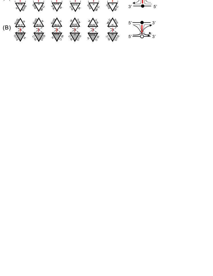
In this paper we approach the problem of cross-serial interactions of pk-structures from first principles. We employ an abstraction, that is well known to structural biology [12]: namely, a nucleotide is not a dimensionless object but a triangle and base pairs can be abstracted as untwisted or twisted ribbons connecting two such triangles, see Fig. 1. This observation introduces topology as a natural language for biological structures and leads to the fatgraph model [13]. Our main result is to map a novel recursion on unicellular maps [14] into the classic recursion derived in [2]. I.e. we translate a recursive procedure on fatgraphs into an enhanced version of the recursion of secondary structures. This results in the first, unambiguous, context-free grammar for pk-structures, RNAFeatures∗. We present as a first application an Boltzmann sampler and stochastic context-free grammar.
In the following we discuss the fatgraph modeling Ansatz in detail. We then provide some background on computational linguistics in the context of RNA structures, enabling us to discuss what we mean by topological language of RNA.
The biophysics of the canonical base pairs A-U, G-C and G-U implies, that the fatgraphs modeling RNA structures are orientable: RNA purine and pyrimidine bases are modeled as three edges for hydrogen bonding interactions: the Watson-Crick edge, the Hoogsteen edge, and the Sugar edge111which includes the 29-OH and which has also been referred to as the Shallowgroove edge [12]. A given edge of one base can potentially interact in a plane with any one of the three edges of a second base, and can do so in either cis- or trans- orientation of the glycosidic bonds. This gives rise to 12 basic geometric types with at least two H bonds connecting the bases, see Fig. 1. Accordingly, cis-base pairs, including the canonical base pairs belong to the cis-Watson-Crick/Watson-Crick geometry.
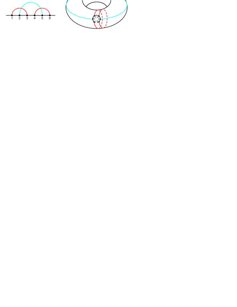
Canonical base pairs induce exclusively untwisted ribbons, modeled via orientable fatgraphs, i.e. graphs enhanced by replacing vertices by discs and edges by ribbons. Gluing the sides of these ribbons produces the topological quotient space [15], which is a connected sum of tori. As topological genus, , and orientability are the two determinants of closed surfaces, RNA structures having canonical base pairs are filtered by genus alone. RNA secondary structures [16], are exactly structures of genus zero. Structures of genus are those exhibiting cross-serial interactions. In a sense, topological genus measures the complexity of a biomolecule, far more subtle than the number of crossing arcs. One may think of pk-structures as cross-free drawings on a closed surface of genus , instead of a drawing with crossing arcs in the plane222A cross-free drawing in the plane corresponds to an RNA secondary structure., see Fig. 2.
The term language of RNA has been used in [17], where the authors study the aforementioned gap-structures [11]. Methods from computational linguistics have been applied to problems in DNA and RNA sequence analysis for decades: early work involved using regular grammars and hidden Markov models (HMMs) in order to model biological sequences. These have been used in sequence analysis [18], such as identifying CpG islands [19], gene prediction [20], pairwise and multiple sequence alignment [19, 21], modeling DNA sequencing errors [22], protein secondary structure prediction, and RNA structural alignment [23]. Regular grammars and HMMs are not well-equipped to model problems in RNA folding because they cannot describe the long-distance correlations of base pairs. Instead, a larger class called context-free grammars (CFG) are used. Assigning probabilities to the production rules of CFG produces a stochastic context-free grammar (SCFG), which, in the context of HMM, allows each state to generate not a single, but any (fixed) number of immediate successors.
By a topological language of RNA we mean an unambiguous, CFG that allows us to recursively construct any pk-structure using recursions that are induced by cell-surgery on fatgraphs. The latter shall be translated into an enhancement of the classical recursion [2]. This allows us to connect to the existing paradigm by presenting a CFG based on arc-removals and decomposition as production rules333as for CFG of secondary structures, where the cross-serial interactions are encapsulated in the labels of the arcs and nonterminal symbols, respectively.
Finally we discuss the above mentioned recursion of secondary structures and provide some background on topological RNA structures.
Waterman et al. [24, 2, 25, 26] studied the combinatorics and folding of RNA secondary structures. Their diagrams are labeled graphs over the vertex set , presented by drawing the vertices on a horizontal line and noncrossing arcs in the upper half-plane. Vertices and arcs correspond to the nucleotides A, G, U and C and Watson-Crick (A-U, G-C) and wobble (U-G) base pairs, respectively. The noncrossing arcs of RNA secondary structures allow for a recursive build. Let denotes the number of RNA secondary structures over nucleotides then we have [24]: , where for . Accordingly, RNA secondary structures satisfy a constructive recursion. This relation constitutes the basis for the DP-recursions used for the polynomial time folding [16, 4] and has profound algorithmic implications. The DP-framework has ever since strongly influenced the field of RNA folding [24, 4, 27, 5].
CFGs of secondary structures [4, 5, 28] are utilizing the recursive nature of secondary structures [24]. The grammar has two production rules, displayed in Fig. 3. Its terminal symbols denote a pair of vertices forming an arc as well as an unpaired vertex and the nonterminal symbols are an arbitrary secondary structure and an irreducible structure covered by an external arc. The grammar is unambiguous, i.e. each structure has a unique decomposition path.
Cross-serial interactions or pseudoknots have long been known as important structural elements [29, 30] in RNA. Depicting a contact structure as a diagram, a structure contains a pseudoknot if and only if these arcs cross. Cross-serial interactions are functionally important in tRNAs, RNaseP [31], telomerase RNA [32], and ribosomal RNAs [33]. Pseudoknots in plant virus RNAs mimic tRNA structures, and in vitro selection experiments have produced pseudoknotted RNA families that bind to the HIV-1 reverse transcriptase [34].
Topological RNA structures have been introduced in [35, 36] and the classification and expansion of pk-structures in terms of the topological genus of an associated fatgraph has been studied by means of matrix theory in [37, 38]. The computation of the genus of a fatgraph is classic [39] and was first applied to RNA structures by [37] and [38]. [40] studies topological RNA structures of higher genus and connects them with Riemann’s Moduli space [36]. In [41] a polynomial time, loop-based folding algorithm of topological RNA structures was given.
2 Fatgraphs and blueprints.
The contacts of nucleotides within an RNA structure can be represented as a diagram whose arcs can be linearly ordered via their left end-points, i.e. if and only if . Suppose , then and cross iff holds.
In the following we shall assume that any diagram contains the arc (rainbow), which is not accounted for as an edge of the diagram. Rainbows mark the start and endpoint of the - oriented backbone, thus allowing to collapse the backbone into a disc without loosing any information.
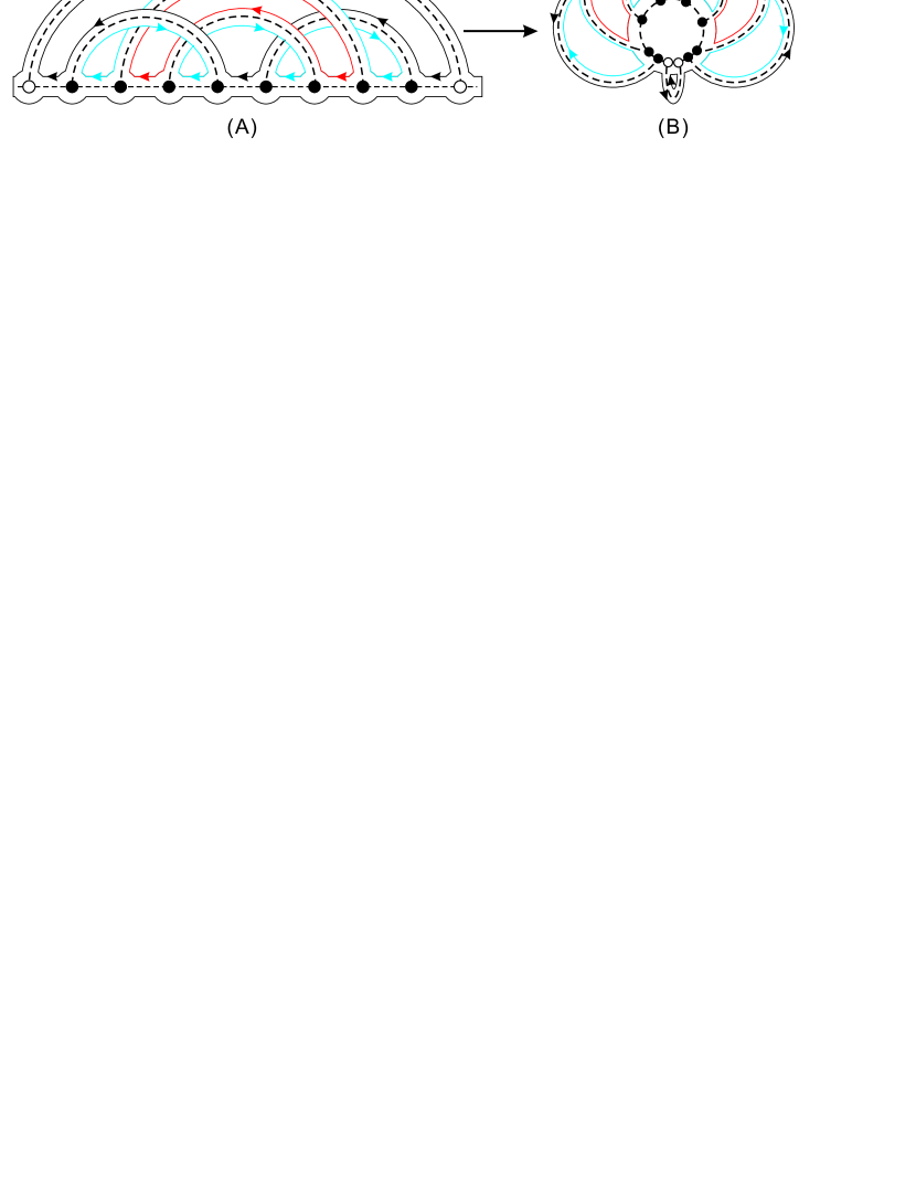
The passage from diagrams to fatgraphs [42, 13] is obtained by “thickening” the edges into (untwisted) bands or ribbons. Furthermore, each vertex is inflated into a disc as shown in Fig. 4. This inflation reflects the fact that canonical base pairs fix a plane, see Fig. 1. A fatgraph, , can thus be viewed as a “drawing” on an orientable surface , which is obtained by identifying the sides of the ribbons. is a -dimensional cell complex over its geometric realization, .
The Euler characteristic and topological genus of the surface are given by and , where , and denote the number of discs, ribbons and boundary components in [15]. The equivalence of simplicial and singular homology [43] implies that these combinatorial invariants are topological invariants. This means the genus of the surface provides a filtration of fatgraphs.
A fatgraph can be presented by a pair of permutations [13]. Let denote the set of half-edges, and let , and be three permutations over , where each cycle in , and presents a vertex, an edge and a boundary component, respectively. A vertex of degree is considered as a cycle . In particular, is a fixed-point free involution since an edge consist of two half-edges and we have .
Removing the unpaired vertices from the diagram and collapsing the backbone into a disc does not change the Euler characteristic. Therefore, the relation between genus and number of boundary components is solely determined by the number of arcs in the upper half-plane: , where is number of arcs and the number of boundary components. The latter can be computed easily and allows us to obtain the genus of the diagram.
Mapping into , is a bijection, see Fig. 5. is called the Poincaré dual and interchanges boundary components with vertices, preserving topological genus. By construction we shall deal only with fatgraphs over one backbone whose duals thus have one boundary component. We refer to these duals as unicellular maps.
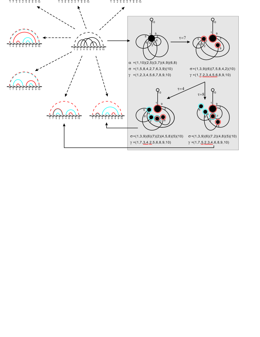
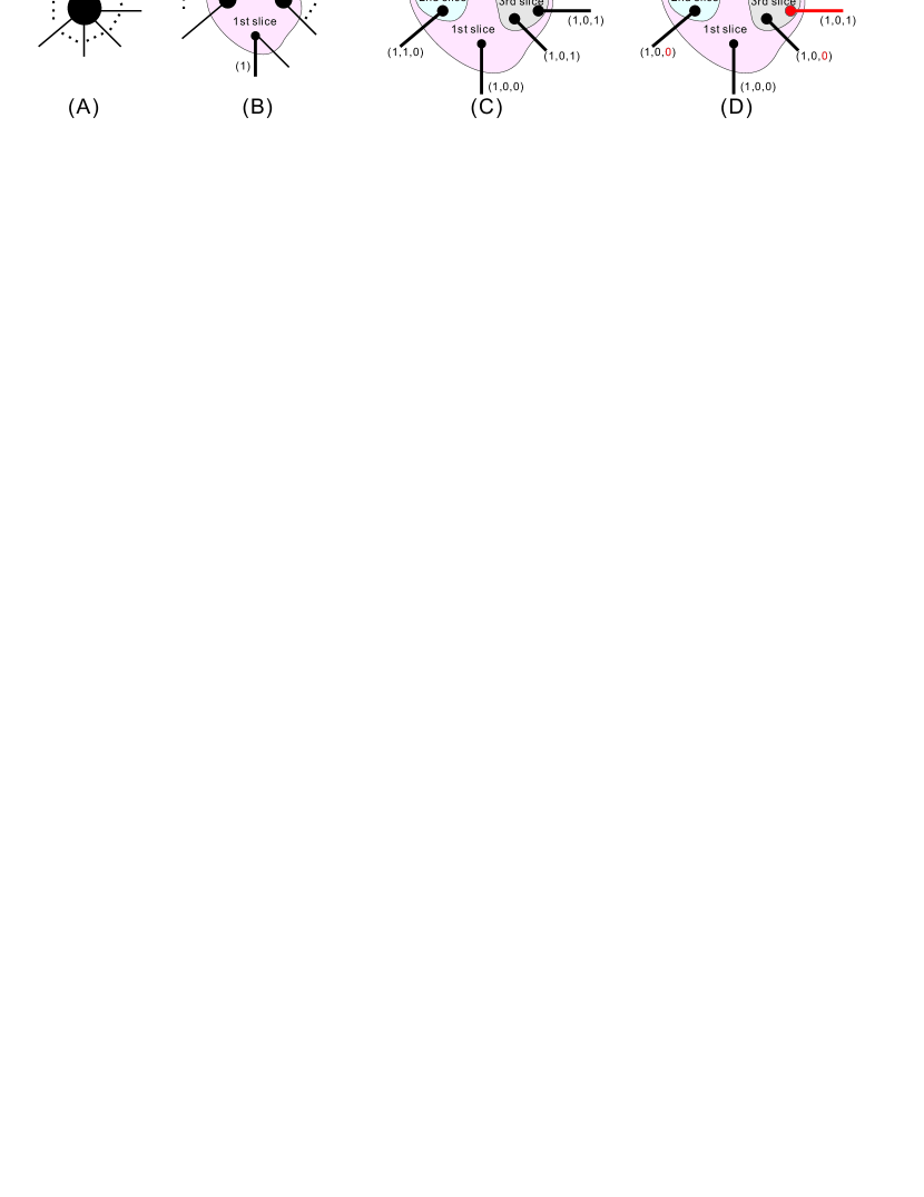
A bijection is derived by Chapuy in [14] between a unicellular map of genus together with a distinguished trisection and a unicellular map of genus , together with labeled vertices. This is facilitated by successively slicing a vertex into three new vertices via the distinguished trisection. Since the trisection can persist through finitely many slicings, say times, the process produces labeled vertices, reducing the genus of the map by exactly . Gluing is the inverse to slicing: gluing a set of labeled vertices in a unicellular map increases the genus of the map by . By construction, both, slicing and gluing processes preserve unicellularity.
In a unicellular map we have two orders, and . The former accounts for the length of the tour of the boundary component and the latter is induced by counterclockwise rotation around a vertex, i.e. from to . A half-edge is called a trisection if and is not the minimum half-edge of the vertex. A trisection marks the nontrivial order discrepancies between and . It is topologically relevant, since the number of trisections in any unicellular map having genus equals exactly [14]. In particular, any unicellular map having genus , i.e. a planar tree, has no trisections.
Let be a vertex with trisection . We slice as follows [14]: let denote the minimum half-edge of , let denote the minimum half-edge between and (rotating clockwise), that is larger than with respect to . Iterating this means to further slice until becomes its minimum half-edge and we derive the mapping , where denotes the number of slicings. The new vertices are by construction ordered by their minimum half-edges with respect to . Furthermore, is bijective.
The process can be reversed, i.e., , derived by successively gluing in the following fashion: we first glue the last three vertices , and obtaining a new vertex, , with an (intermediate) trisection. Continuing this, by gluing the next two vertices with , produces a unicellular map together with the trisection . Iterated slicings and selecting new trisections as needed, generates a unicellular map having genus , i.e. a planar tree.
Definition 1.
(blueprint) Suppose is a unicellular map of genus having edges together with the trisection . A -blueprint is a sequence
where , for and .
Remark 1.
In the following we shall refer to the blueprint of the dual of a pk-structure simply as the blueprint of the pk-structure. In Fig. 6 we display the blueprints of a matching having genus .
Remark 2.
Note that for two unicellular maps having genus , the number of blueprints is not necessarily equal. Furthermore, all blueprints can be constructed by considering all trisections at each step, respectively. The cost of finding all blueprints is exponential in , however, the genus of RNA structures found in databases is typically less than .
3 -structures
We establish now a bijection between unicellular maps together with blueprints and a particular class of labeled, planar trees. The labels will allow to recover the blueprints. Note that, since some vertices may have been involved in subsequent slicing events, they are not present in the tree.
Definition 2.
(-tree)
A -tree, is a rooted, planar tree with boundary component
, in which a vertex carries the label such that
, where ,
,
and any vertex, whose label satisfies
for , is minimal in within the set of all the vertices, having label where
.
We shall call the minimum vertex with the property transitional of level and regular, otherwise. Note that a vertex can be transitional for multiple indices.
Lemma 1.
Any unicellular map, , together with a blueprint, , induces a unique -tree, .
Proof.
Suppose we are given a unicellular map together with a slice-path consisting of slicings. generates a planar tree, , whose vertices we color red if they were involved in some slicing and black, otherwise. furthermore specifies the sequence of slicings and each slicing reduces topological genus by at least one, whence .
We label the black vertices by and each red vertex obtains a in its th-coordinate if and only if it was involved in the th-slicing. This produces a set of intermediate labels .
We proceed by reducing the : starting from to , we set
Accordingly, any -minimal vertex of a fixed slicing retains a iff it came from a previously sliced vertex and, as a result, irrespective of how many times the vertices were sliced, the total number of entries in all coordiantes of all lables equals:
where is the decrease of genus in the th slicing. As a result, we have .
By construction, the total number of entries found as th-coordinates equals the total number of vertices obtained via the th slicing, whence .
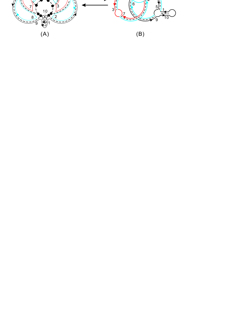
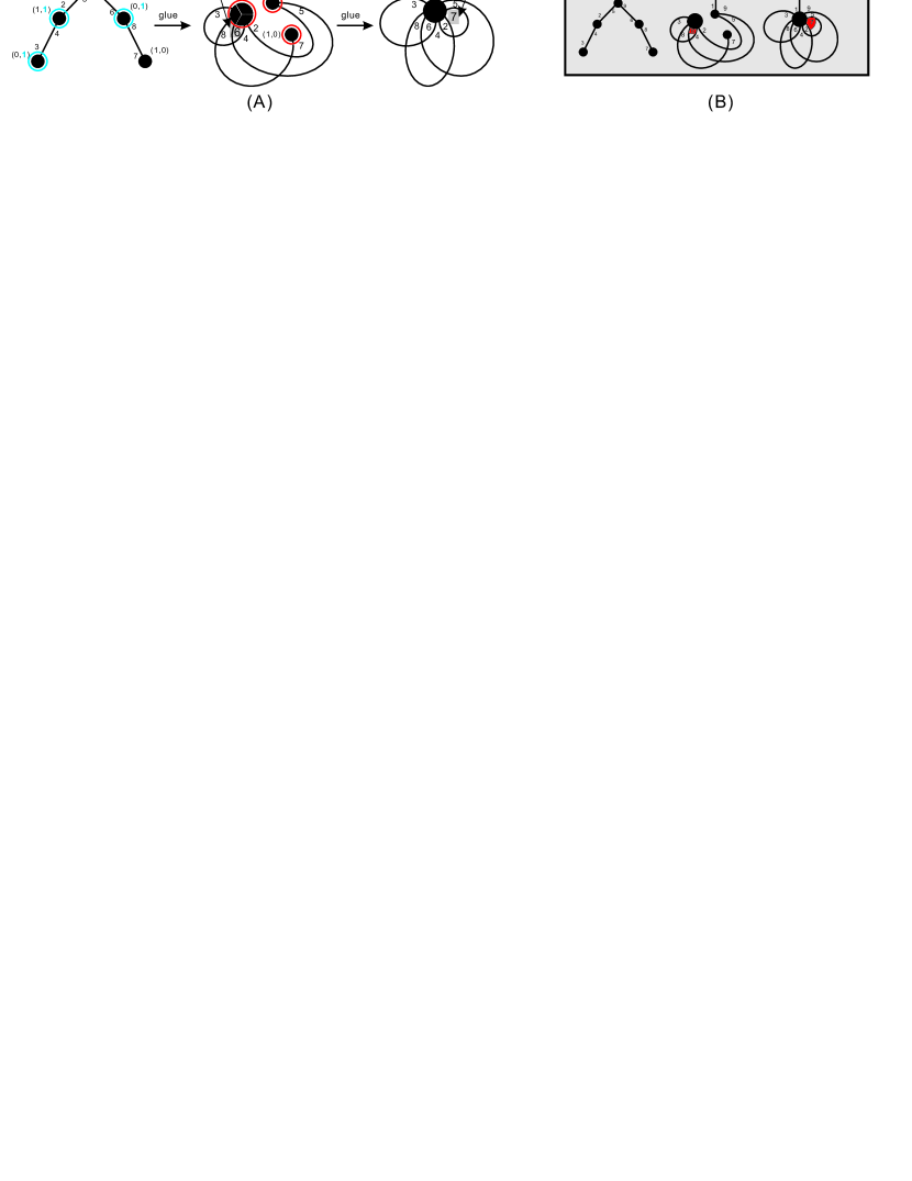
Finally, consider two fixed indices . Only the label of the -minimal vertex amongst the vertices of the th slicing can have an entry as th coordinate, whence and the proof of the lemma is complete. In Fig. 7 we illustrate the idea of the proof. ∎
Having established the mapping from unicellular maps of genus together with blueprints into -trees, we proceed by showing that this mapping is bijective.
Proposition 1.
Suppose is a unicellular map with genus and blueprint , then we have the bijection
Proof.
Following the slice-path, , the fatgraph is sliced to the tree with labels , . By Lemma 1, is a -tree, whence is well-defined.
To show that is bijective, let be an arbitrary -tree such that . We shall construct as follows:
Let denote the set of vertices whose labels satisfy . Lemma 1 guarantees that the number of vertices contained in is odd. Then we glue
creating the trisection, , where .
By construction is a unicellular map with two types of vertices: those which correspond to -vertices (type ) and a unique new vertex obtained by gluing the set (type ). We now label the -vertices with labels using the labels of as follows: For any type vertex we set for and . The unique type vertex obtains the label
In Fig. 8 we illustrate the idea of the proof. ∎
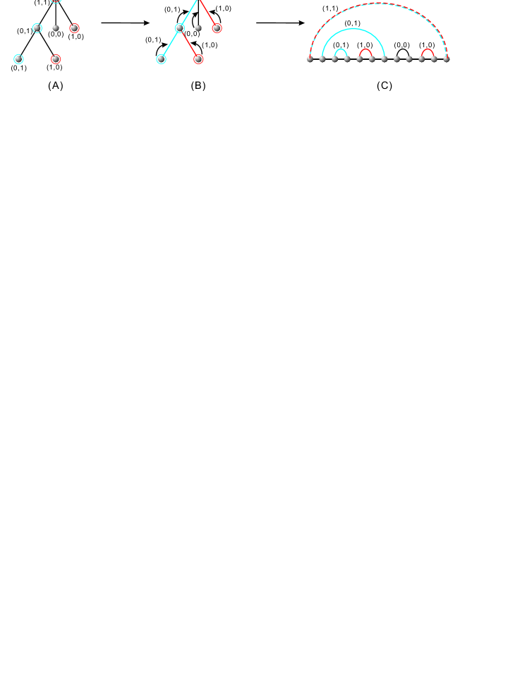
A -tree corresponds to a unicellular map of genus , together with a blueprint. As a planar tree it corresponds by Poincaré duality to a noncrossing matching. We call the edge-labeled Poincaré dual of a -tree a -matching, , whose edge-labels are induced by the vertex labels of the -tree as follows: there are vertices and edges in a planar tree, whence a vertex corresponds uniquely to an edge (except of the root). To this end, we consider the edge which connects to its parent, see Fig. 9. Note that, by construction, the root of the planar tree is never involved in slicings and accordingly labeled .
A -matching induces an arc-labeled secondary structure by insertion of unpaired vertices. To facilitate this we employ the index map , . We interpret as to specify how many unpaired vertices follow the -vertex, . Starting with the left-endpoint of the rainbow and we have such vertices.
Definition 3.
A -structure is a noncrossing diagram with labeled arcs, , that when removing all unpaired vertices, induces a -matching.
Note that slicing induces transpositions of the boundary component. Thus, taking the Poincaré dual, these transpositions permute the backbone of . Let denote resulting permutation of the backbone, where , then is the induced index map for the pk-structure corresponding to the -structure and we have the following situation, see Fig. 10.
4 The grammar
We can now derive the CFG for -structures, RNAFeatures∗. The key issue here will be the compatibility of the arc labels with the production rules.
Let us briefly review the CFG for secondary structures, implied by the recursion of [24], i.e. the tuple , where are sets of nonterminal symbols, terminal symbols and production rules, respectively. A production rule is a mapping from to , where the asterisk represents the Kleene star operation and is an initial symbol. A derivation starts with the initial symbol , and in each step, replaces one of the nonterminal symbols by one of the productions. For secondary structures, the grammar consists of , , and the two production rules are
| (1) |
Here is the -production. The terminal symbols , represent pairs of vertices forming arcs and an unpaired vertex, respectively. The nonterminal symbol denotes an arbitrary structure and is an irreducible structure, i.e. covered by an external arc. Via the initial symbol this grammar is unambiguous, i.e. each structure has a unique derivation path.
We shall now extend the grammar to -structures. To this end we introduce new nonterminals, and . The nonterminal symbols stand for sets of substructures , with labeled arcs such that , . Aside from we have new terminals where denote -labelled arcs. We set if and only if the corresponding nonterminal contains a transitional arc for and , otherwise.
By construction, the will evolve depending on the presence of transitional arcs, that is may change in more than one coordinate if a transitional arc is present, or in at most one coordinate, otherwise. can be viewed as an indicator determining which production rule applies.
Decomposition: this means to decompose a nonterminal symbol
into one left- and one right-symbol, together with consistent labelings.
A labeling for is consistent if
and . Furthermore, consistency for
means
(a) and implies ,
(b) and implies and
(c) implies .
This is a consequence of transitional arcs being induced by transitional vertices by means
of Poincaré duality and the latter being minimal in the boundary component. As a result
a transitional arc needs to be placed in the left-nonterminal as long as the latter contains
any arcs with the property .
As a result we have the production rule:
| (2) |
satisfying , for , , . In case of , if , we have and . Otherwise, if , the th trans-arc is distributed to the right and we have and . Finally, if , both, , see Fig. 11.
Arc-removal: this means to act on the nonterminal by removing its outer arc, . The key point here is to provide this arc with a label, consistent with the label associated with the generated nonterminals. Given any arc-removal based production rule generates the nonterminal , where and . This implies for the label of the removed arc , . In case is a trans-arc for , we have , or , otherwise. Accordingly, we have:
| (3) |
The terminal symbols , nonterminal symbols , production rules given by eq. [2], eq. [3], together with the initial condition with and , for , define the context-free grammar .
Proposition 2.
The context-free grammar discussed above generates all -structures uniquely, or equivalently, all pk-structures together with a blueprint.
Proof: Consider a nonterminal symbol where the are positive odd integers, with and . Any nonterminal symbol is uniquely generated by since the product of each production rule is unique. Furthermore, no labeled arc with can be further added to the structure when is set to be . This guarantees that the trans-arc of level is minimal among those arcs with . Thus the structures generated from are -structures. As for its generative power, an arbitrary a -structure, is translated via into a unique sequence of terminal symbols, whence the proposition.
The grammar for -structure is designed based on the simple grammar for secondary structure by assigning labels to symbols. However, the latter evaluates arcs against unpaired vertices, lacking the capability of differentiating base pairs and unpaired bases in the context of specific loop types.
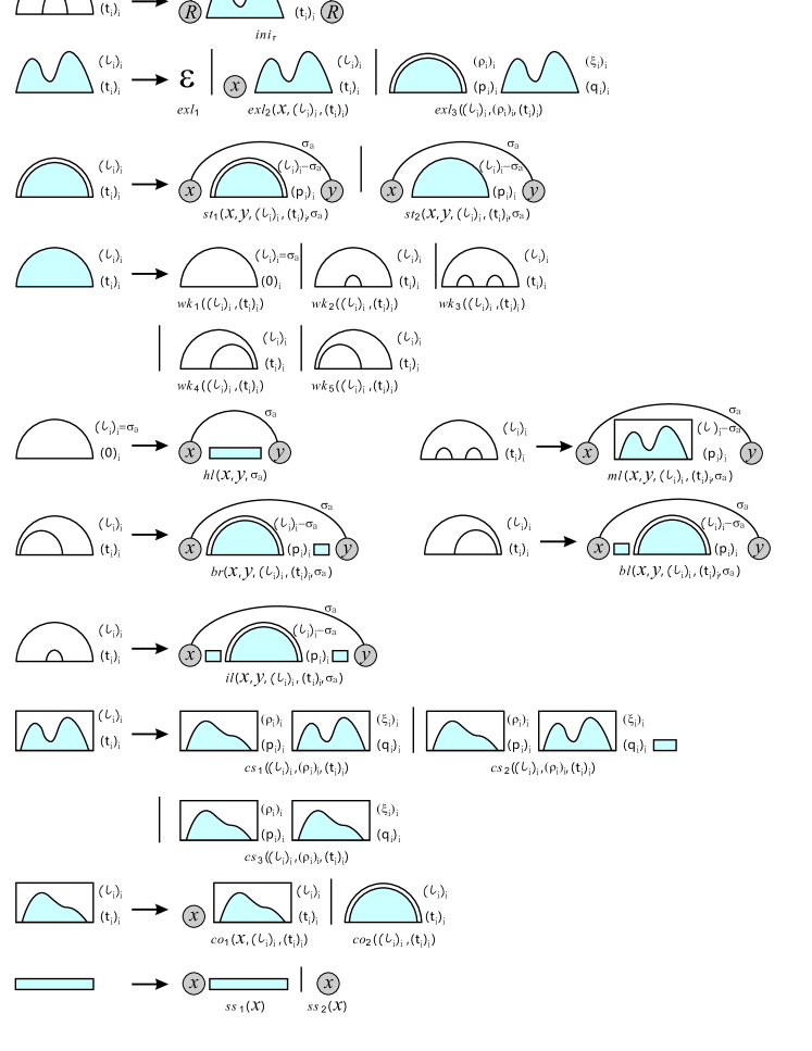
We accordingly present a grammar for -structures, RNAFeatures∗ used in practice that differentiates loop types, that is an extension of the grammar RNAFeatures [44]. The grammar allows us to differentiate loop-types. First we have the terminal symbols representing the respective RNA nucleotides and the endpoint of the rainbow. The nonterminal symbols are
The nonterminal symbols are referenced via both: their semantics and their arc-label information of the class of structures it represents. -structure are -structures corresponding to a pk-structure of genus , together with a blueprint. For nonterminal symbols the , where
the index represents the sum of the arc-labels contained in the class, such that if and only if the transitional arc of level is present. We distinguish the following classes:
-
1.
denotes the class that is immediately nested in the rainbow,
-
2.
denotes the class covered by parallel arcs, while represents the class covered by a isolated arc,
-
3.
represents the class containing no arcs, immediately nested in , while , , have one and have more than one such arc. The classes , and differ in the number of unpaired bases in the two intervals formed between the outer arc and the immediately nested arc. has the interval to the right empty and the intervals to the left non-empty, is defined analogously and in both these intervals are non-empty,
-
4.
and are classes contained in a multi-loop: has exactly one braching and has at least two,
-
5.
denotes the class consisting of a sequence of unpaired bases.
The nonterminal symbols are listed in Fig. 12
-
1.
: here we have . In case of , the rainbow is always a transitional arc, hence if ,
-
2.
emits the signal of the -structure,
-
3.
cuts off the leftmost unpaired base and keeps all the labels as well as transitional arcs in the right nonterminal, where . , and are defined analogously,
-
4.
decompose into two classes, distributing any labeled arcs and in particular any trans-arcs, whence . In case of , if , we have and . Otherwise, if , the th trans-arc is distributed to the RHS and we have and . Finally, if , both, . The rules , and are defined analogously,
-
5.
remove a base pair with the arc label , , inducing the labels for the class produced. If and , the arc is a trans-arc of level and we set accordingly. The rules , , , , as well as , are defined analogously.
We display the production rules in Fig. 13.
Let be a structure and be an RNA sequence. A CFG allows to assign a score to a pair , derived from scores assigned to the production rules encountered. Namely, for each the CFG provides a unique parse tree and the score of is then computed by means of the scores of the respective production rules. Scores based on a thermodynamic energy model produces the minimum free energy (mfe) model [45, 46, 47] and a probabilistic scoring scheme derived from data bases of RNA sequences and structures leads to a SCFG . In the latter case, sequence–structure pairs of the data set allow to assign scores to the production rules, which in turn induce a score of an arbitrary pair .
5 The SCFG of RNA pseudoknot structures
Stochastic context-free grammars (SCFG) were developed for RNA secondary structures [48, 49]. They have been employed for the ab initio structure prediction as well as the analysis of observables such as base pairing probabilities or loop patterns [50, 51, 52]. A SCFG is derived from a CFG by associating to each production rule a probability . That is, for any nonterminal , suppose that are all derivations of , then we have .
Let denotes an RNA structure of genus and be a sequence. For , is a secondary structure and can be parsed by RNAFeatures. We construct the parse tree of and record the frequency of the production rules. In case of , for any -blueprint, , we consider the correspondence
| (4) |
where is a -structure and is the modified sequence. We construct the parse tree of RNAFeatures∗ of and record the frequency of the encountered production rules.
If there are -blueprints, the contribution of each pair is normalized by and the frequency of a production rule equals where is the frequency of being applied. After processing all structures and sequences, the probability of a production rule is computed as the quotient of its frequency over the sum of all frequencies of its respective derivation.
We next consider , the normalized score of an arbitrary structure, , over an arbitrary sequence, , as a function of the data set . We set , where is calculated by the multiplying the probabilities of the production rules in the parse tree of and the sum is taken over the set of all -blueprints.
The induce . Using the fact that for fixed blueprint, , we have a bijection , we derive
Furthermore the SCFG facilitates the sampling of structures with Boltzmann probability, i.e., . We employ RNAFeatures∗ to Boltzmann sample a -structure , and reconstruct as well as the associated blueprint, : fixing , suppose there are blueprints , these correspond to the distinct -structures . Let be the collection of all such . In view of being a bijection, we have
Therefore, in view of and
we have .
As for runtime complexity, the Boltzmann sampler of secondary structures using such a SCFG has runtime of , if structures are ranked according to the sequential order. This can be improved to by ranking the structures with the Boustrophedon order [53, 9]. For fixed topological genus, the label enhancement of RNAFeatures∗ by construction increases only the number of derivations. Thus the Boltzmann sampler for -structures has runtime complexity .
6 Discussion
RNA secondary structures have been widely studied using the classic CFG implied by the recursions in [16, 24]. Using RNA sequence and structure data sets, this CFG induces a SFCG. This SCFG has been applied for the ab initio prediction of RNA secondary structures [28, 50], calculating the likelihood of a sequence generated by the model SCFG [51], and detecting RNA genes using comparative sequence analysis [52]. Furthermore, the generation of random secondary structures according to the native distributions of certain families of RNA structures is studied in [9] in order to identify key structural motifs in biological RNA secondary structures. This paper allows to extend these studies to pk-structures. To the best of our knowledge RNAFeatures∗ is the first unambiguous context-free grammar for pk-structures. Related work has been done by Freiermuth and Nebel on a CFG of certain, colored trees. These are trees that can be mapped to unicellular maps, however, not bijectively.
A particular, multiple context-free grammar (MCFG) for pk-structures is introduced in [11]. This grammar employs a vector of nonterminal symbols referencing a substructure with a gap. The time and space complexity for Boltzmann sampling pk-structures with this grammar are and , respectively. The grammar furthermore implies a folding algorithm having relatively high computational cost [11]: time and space complexity, using the thermodynamic model. Restricting to certain types of pk-structures the time complexity can be reduced to time complexity [54]. In any case, specifying the output space of the MCFG, i.e. what types of structures the grammar actually generates is subtle, see [17] for details.
The passage from MCFG to CFG has implications for time and space complexity: an MCFG contains rules of the type where , are vectors of nonterminals. It requires a minimum of three loop-indices to execute these rules in the sampling or folding process. In contrast, the production rule in any CFG being in Chomsky normal form can be written as , which requires only one loop index, reducing the time complexity by . As for space complexity this passage obsoletes using vectors, reducing the space complexity for and for sampling and folding, respectively.
The key idea facilitating this passage lies in mapping the information of crossing arcs into the labels of noncrossing arcs, i.e. passing from pk-structures to -structures. Accordingly, the bijection of eq. 4 is the crucial point. The fact that the bijection is genuinely topology-based allows RNAFeatures∗ to extend the classic CFG of secondary structures, generating any pk-structure.
In the following we present the expectation and variance of some important parameters related to the structural features of pk-structures generated by the induced SCFG of RNAFeatures∗. These parameters are also used to analyze Boltzmann sampled secondary structures in comparison with native structures in [9]. Our SCFG is trained via single stranded tRNA sequence-structure pairs, taken from the Nucleic Acid Database (NDB) [55, 56], considering only Watson-Crick and wobble base pairs. In this training set, we find structures having genus , of genus and structure of genus . The average sequence length is nucleotides. We analyze the following five random variables: , the number of base pairs, , the number of stacks, , the average length of a stack, , the number of hairpin and finally , the average length of a hairpin loop. Here a stack of length is the maximal sequence of parallel arcs . A hairpin loop of length is a substructure, which consists of a base pair and the unpaired bases .
The statistics is obtained by Boltzmann sampling of structures over nucleotides via the SCFG. For reference purposes we furthermore sample random structures over nucleotides, having fixed genus and , respectively, with uniform probability [57]. We summarize in Table 1 the respective means and variances of the above five random variables.
The sampling generates , , structures having genus , and , reflecting the large quantity of genus structures in the training set. By construction our SCFG does not recognize contributions of unpaired bases in hairpin loops, bulges and interior loops, which explains the systematic deviation in the lengths of hairpin-loops. Table 1 shows that the Boltzmann sampled structures are not random structures of either genus zero or one.
The implication of the CFG to the folding of pk-structures is work in progress. Though we can fold a -structure over a given sequence in time, the bijection producing the corresponding pseudoknotted structure does systematically alter the underlying sequence. In particular, in case of pk-structures of genus one, this consists in the transposition of two subsequent intervals and is thus manageable.
7 Acknowledgments.
We gratefully acknowledge the help of Kevin Shinpaugh and the computational support team at VBI. Many thanks to Christopher L. Barrett and Henning Mortveit for discussions.
References
- [1] O. C. Uhlenbeck, A coat for all sequences, Nature Struct. Biol. 5 (1998) 174–176.
- [2] P. R. Stein, M. S. Waterman, On some new sequences generalizing the catalan and motzkin numbers, Discrete Math. 26 (1978) 261–272.
- [3] M. S. Waterman, T. F. Smith, Rapid dynamic programming methods for RNA secondary structure, Adv. Appl. Math. 7 (1986) 455–464.
- [4] M. Zuker, P. Stiegler, Optimal computer folding of larger RNA sequences using thermodynamics and auxiliary information, Nucleic Acids Res. 9 (1981) 133–148.
- [5] I. L. Hofacker, W. Fontana, P. F. Stadler, L. S. Bonhoeffer, M. Tacker, P. Schuster, Fast folding and comparison of RNA secondary structures, Monatsh. Chem. 125 (1994) 167–188.
- [6] J. S. McCaskill, The equilibrium partition function and base pair binding probabilities for RNA secondary structure, Biopolymers 29 (1990) 1105–1119.
- [7] P. Duchon, P. Flajolet, G. Louchard, G. Schaeffer, Boltzmann samplers for the random generation of combinatorial structures, Combinatorics, Probability and Computing 13 (2004) 2004.
- [8] M. A. Harrison, Introduction to Formal Language Theory, Addison-Wesley, 1978.
- [9] M. E. Nebel, A. Scheid, F. Weinberg, Random generation of RNA secondary structures according to native distributions, Algorithms Mol. Biol. 6 (24) (2011) doi:10.1186/1748–7188–6–24.
- [10] W. Fontana, D. A. M. Konings, P. F. Stadler, P. Schuster, Statistics of RNA secondary structures, Biopolymers 33 (1933) 1389–1404.
- [11] E. Rivas, S. R. Eddy, A dynamic programming algorithm for RNA structure prediction including pseudoknots, J. Mol. Biol. 285 (1999) 2053–2068.
- [12] N. B. Leontis, E. Westhof, Geometric nomenclature and classification of RNA base pairs, RNA 7 (2001) 499–512.
- [13] R. C. Penner, M. Knudsen, C. Wiuf, J. E. Andersen, Fatgraph models of proteins, Comm. Pure Appl. Math. 63 (2010) 1249–1297.
- [14] G. Chapuy, A new combinatorial identity for unicellular maps, via a direct bijective approach, Adv. Appl. Math. 47(4) (2011) 874–893.
- [15] W. S. Massey, Algebraic Topology: An Introduction, Springer-Veriag, New York, 1967.
- [16] T. Smith, M. Waterman, RNA secondary structure, Math. Biol. 42 (1978) 31–49.
- [17] E. Rivas, S. R. Eddy, The language of RNA: A formal grammar that includes pseudoknots, Bioinformatics 16 (2000) 334–340.
- [18] L. Pachter, B. Sturmfels, Algebraic Statistics for Computational Biology, Cambridge University Press, 2005.
- [19] R. Durbin, S. R. Eddy, A. Krogh, G. Mitchison, Biological Sequence Analysis. Cambridge, Cambridge University Press, 1998.
- [20] K. Munch, A. Krogh, Automatic generation of gene finders for eukaryotic species, BMC Bioinformatics 7 (2006) 263.
- [21] L. Pachter, M. Alexandersson, S. Cawley, Applications of generalized pair hidden markov models to alignment and gene finding problems, J. Comput. Biol. 9 (2) (2002) 389–99.
- [22] C. Lottaz, C. Iseli, C. V. Jongeneel, P. Bucher, Modeling sequencing errors by combining hidden markov models, Bioinformatics 19 Suppl 2 (2003) ii103–12.
- [23] B. J. Yoon, P. P. Vaidyanathan, Structural alignment of RNAs using profile-csHMMs and its application to RNA homology search: Overview and new results., IEEE Trans. Automat. Contr. (Joint Special Issue on Systems Biology with IEEE Transactions on Circuits and Systems: Part-I) 53 (2008) 10–25.
- [24] M. S. Waterman, Secondary structure of single-stranded nucleic acids, Adv. Math. (Suppl. Studies) 1 (1978) 167–212.
- [25] R. Nussinov, G. Piecznik, J. R. Griggs, D. J. Kleitman, Algorithms for loop matching, SIAM J. Appl. Math. 35 (1) (1978) 68–82.
- [26] D. Kleitman, Proportions of irreducible diagrams, Studies in Appl. Math. 49 (1970) 297–299.
- [27] D. Sankoff, G. Leduc, N. Antoine, B. Paquin, B. F. Lang, C. R., Gene order comparisons for phylogenetic inference: Evolution of the mitochondrial genome, Proc. Natl. Acad. Sci. USA 89 (1992) 6575–6579.
- [28] B. Knudsen, J. J. Hein, Using stochastic context-free grammars and molecular evolution to predict RNA secondary structure, Bioinformatics 15 (1999) 446–454.
- [29] E. Westhof, L. Jaeger, RNA pseudoknots, Curr. Opin. Struct. Biol. 2 (1992) 327–333.
- [30] J. L. Chen, C. W. Greider, Functional analysis of the pseudoknot structure in human telomerase RNA, Proc. Natl. Acad. Sci. USA 102 (23) (2005) 8080–5.
- [31] A. Loria, T. Pan, Domain structure of the ribozyme from eubacterial ribonuclease, RNA 2 (1996) 551–563.
- [32] D. W. Staple, S. E. Butcher, Pseudoknots: RNA structures with diverse functions, PLoS Biol. 3 (2005) e213.
- [33] D. Konings, R. Gutell, A comparison of thermodynamic foldings with comparatively derived structures of 16s and 16s-like rRNAs, RNA 1 (1995) 559–574.
- [34] C. Tuerk, S. MacDougal, L. Gold, RNA pseudoknots that inhibit human immunodeficiency virus type 1 reverse transcriptase, Proc. Natl. Acad. Sci. USA 89(15) (1992) 6988–6992.
- [35] R. C. Penner, M. S. Waterman, Spaces of RNA secondary structures, Adv. Math. 101 (1993) 31–49.
- [36] R. C. Penner, Cell decomposition and compactification of Riemann’s moduli space in decorated Teichmüller theory, in: N. Tongring, R. C. Penner (Eds.), Woods Hole Mathematics-perspectives in math and physics, World Scientific, Singapore, 2004, pp. 263–301, arXiv: math. GT/0306190.
- [37] H. Orland, A. Zee, RNA folding and large matrix theory, Nuclear Physics B 620 (2002) 456–476.
- [38] M. Bon, G. Vernizzi, H. Orland, A. Zee, Topological classification of RNA structures, J. Mol. Biol. 379 (2008) 900–911.
- [39] L. Euler, Elementa doctrinae solidorum, Novi Comm. Acad. Sci. Imp. Petropol 4 (1752) 109–140.
- [40] J. E. Andersen, R. C. Penner, C. M. Reidys, M. S. Waterman, Topological classification and enumeration of RNA structrues by genus, J. Math. Biol. 67 (5) (2013) 1261–1278.
- [41] C. M. Reidys, F. Huang, J. E. Andersen, R. C. Penner, P. F. Stadler, M. E. Nebel, Topology and prediction of RNA pseudoknots, Bioinformatics 27 (2011) 1076–1085.
- [42] M. Loebl, I. Moffatt, The chromatic polynomial of fatgraphs and its categorification, Adv. Math. 217 (2008) 1558–1587.
- [43] A. Hatcher, Algebraic Topology, Cambridge University Press, 2002.
- [44] R. Giegerich, Introduction to stochastic context free grammars, in: J. Gorodkin, W. L. Ruzzo (Eds.), RNA Sequence, Structure, and Function: Computational and Bioinformatic Methods, 1st Edition, Vol. 1097, Humana Press, 2014, Ch. 5, pp. 85–126.
- [45] D. Mathews, J. Sabina, M. Zuker, D. Turner, Expanded sequence dependence of thermodynamic parameters improves prediction of RNA secondary structure, J. Mol. Biol. 288 (1999) 911–940.
- [46] D. Mathews, M. Disney, J. Childs, S. Schroeder, M. Zuker, D. Turner, Incorporating chemical modification constraints into a dynamic programming algorithm for prediction of RNA secondary structure, Proc. Natl. Acad. Sci. USA 101 (2004) 7287–7292.
- [47] D. Turner, D. H. Mathews, NNDB: the nearest neighbor parameter database for predicting stability of nucleic acid secondary structure, Nucl. Acids Res. 38 (2010) D280–D282.
- [48] S. R. Eddy, R. Durbin, RNA sequence analysis using covariance models, Nucl. Acids Res. 22 (1994) 2079–2088.
- [49] Y. Sakakibara, M. Brown, R. Hughey, I. S. Mian, K. Sjöolander, D. Underwood, R. C.and Haussler, Stochastic context-free grammars for tRNA modeling, Nucl. Acids Res. 22 (1994) 5112–5120.
- [50] B. Knudsen, J. J. Hein, Pfold: RNA secondary structure prediction using stochastic context-free grammars, Nucl. Acids Res. 31 (2003) 3423–3428.
- [51] E. Rivas, S. R. Eddy, Secondary structure alone is generally not statistically significant for the detection of noncoding RNAs, Bioinformatics 16 (7) (2000) 583–605.
- [52] E. Rivas, S. R. Eddy, Noncoding RNA gene detection using comparative sequence analysis, BMC Bioinformatics 2 (8).
- [53] Y. Ponty, Efficient sampling of RNA secondary structures from the Boltzmann ensemble of low-energy: the boustrophedon method, J. Math. Biol. 56 (1-2) (2008) 107–27.
- [54] R. M. Dirks, N. A. Pierce, A partition function algorithm for nucleic acid secondary structure including pseudoknots, J. Comput. Chem. 24 (2003) 1664–1677.
- [55] H. M. Berman, W. K. Olson, D. L. Beveridge, J. Westbrook, A. Gelbin, T. Demeny, A. R. Hsieh, S. H. amd Srinivasan, B. Schneider, The nucleic acid database: A comprehensive relational database of three-dimensional structures of nucleic acids, Biophys. J. 63 (751-759).
- [56] B. C. Narayanan, J. Westbrook, S. Ghosh, A. I. Petrov, B. Sweeney, C. L. Zirbel, N. B. Leontis, H. M. Berman, The nucleic acid database: new features and capabilities, Nucleic Acids Res. 42 (2013) D114–22.
- [57] F. Huang, M. E. Nebel, C. M. Reidys, Generation of RNA pseudoknot structures with topological genus filtration, Math Biosci. 245 (2) (2013) 216–225.



| Input Set | Boltzmann | Uniform, | Uniform | |
|---|---|---|---|---|