Comparison of continuous and discrete-time data-based modeling for hypoelliptic systems

Abstract

We compare two approaches to the predictive modeling of dynamical systems from partial observations at discrete times. The first is continuous in time, where one uses data to infer a model in the form of stochastic differential equations, which are then discretized for numerical solution. The second is discrete in time, where one directly infers a discrete-time model in the form of a nonlinear autoregression moving average model. The comparison is performed in a special case where the observations are known to have been obtained from a hypoelliptic stochastic differential equation. We show that the discrete-time approach has better predictive skills, especially when the data are relatively sparse in time. We discuss open questions as well as the broader significance of the results.

Keywords: Hypoellipticity; stochastic parametrization; Kramers oscillator; statistical inference; discrete partial data; NARMA.

1 Introduction

We examine the problem of inferring predictive stochastic models for a dynamical system, given partial observations of the system at a discrete sequence of times. This inference problem arises in applications ranging from molecular dynamics to climate modeling (see, e.g. [10, 12] and references therein). The observations may come from a stochastic or a deterministic chaotic system. This inference process, often called stochastic parametrization, is useful both for reducing computational cost by constructing effective lower-dimensional models, and for making prediction possible when fully-resolved measurements of initial data and/or a full model are not available.

Typical approaches to stochastic parametrization begin by identifying a continuous-time model, usually in the form of stochastic differential equations (SDEs), then discretizing the resulting model to make predictions. One difficulty with this standard approach is that it often leads to hypoelliptic systems [19, 22, 28], in which the noise acts on a proper subset of state space directions. As we will explain, this degeneracy can make parameter estimation for hypoelliptic systems particularly difficult [28, 33, 30], makiing the resulting model a poor predictor for the system at hand.

Recent work [8, 21] has shown that fully discrete-time approaches to stochastic parametrization, in which one considers a discrete-time parametric model and infers its parameters from data, have certain advantages over continuous-time methods. In this paper, we compare the standard, continuous-time approach with a fully discrete-time approach, in a special case where the observations are known in advance to have been produced by a hypoelliptic system whose form is known, and only some parameters remain to be inferred. We hope that this comparison, in a relatively simple and well-understood context, will clarify some of the advantages and disadvantages of discrete-time modeling for dynamical systems. We note that our discussion here leaves in abeyance the question of what to do in cases where much less is known about the origin of the data; in general, there is no reason to believe that a given set of observations was generated by any stochastic differential equation or by a Markovian model of any kind.

A major difficulty in discrete modeling is the derivation of the structure, i.e. of the terms in the discrete-time model. We show that when the form of the differential equation giving rise to the data is known, one can deduce possible terms for the discrete model, but not necessarily the associated coefficients, from numerical schemes. Note that the use of this idea places the discrete and continuous models we compare on an equal footing, in that both approaches produce models directly derived from the assumed form of the model.

Model and goals.

The specific hypoelliptic stochastic differential equations we work with have the form

$$dx_{t} = y_{t}~{}dt,$$ (1.1)

$$dy_{t} = \big{(}-\gamma y_{t}-V^{\prime}(x_{t})\big{)}~{}dt+\sigma dB_{t}~{},$$

where $B_{t}$ is a standard Wiener process. When the potential $V$ is quadratic, i.e.,

$$V(x)=\frac{\alpha}{2}x^{2}~{},~{}~{}\alpha>0,$$

we get a linear Langevin equation. When the potential has the form

$$V(x)=\frac{\beta}{4}x^{4}-\frac{\alpha}{2}x^{2}~{},~{}~{}\alpha,\beta>0,$$

this is the Kramers oscillator [20, 31, 3, 15]. It describes the motion of a particle in a double-well potential driven by white noise, with $x_{t}$ and $y_{t}$ being the position and the velocity of the particle; $\gamma>0$ is a damping constant. The white noise represents the thermal fluctuations of a surrounding “heat bath”, the temperature of which is connected to $\gamma$ and $\sigma$ via the Einstein relation $T=\frac{\sigma^{2}}{2\gamma}$. This system is ergodic, with stationary density $p(x,y)\propto\exp\left(-\frac{2\gamma}{\sigma^{2}}\left(\frac{1}{2}y^{2}+V(x)\right)\right)$. It has multiple time scales and can be highly nonlinear, but is simple enough to permit detailed numerical study. Parameter estimation for this system is also rather well-studied [28, 30]. These properties make Eq. (1.1) a natural example for this paper.

One of our goals is to construct a model that can make short-time forecasts of the evolution of the variable $x$ based on past observations $\left\{{x}_{nh}\right\}_{n=1}^{N}$, where $h>0$ is the observation spacing, in the situation where the parameters $\gamma$, $\alpha$, $\beta$, and $\sigma$ are unknown. (The variable $y$ is not observed, hence even when the parameters are known, the initial value of $y$ is missing when one tries to solve the SDEs to make predictions.) We also require that the constructed model be able to reproduce long-term statistics of the data, e.g., marginals of the stationary distribution. In part, this is because the form of the model (either continuous or discrete-time) is generally unknown, and reproduction of long-term statistics provides a useful criterion for selecting a particular model. But even more important, in order for a model to be useful for tasks like data assimilation and uncertainty quantification, it must faithfully capture relevant statistics on time scales ranging from the short term (on which trajectory-wise forecasting is possible) to longer time scales.

Our main finding is that the discrete-time approach makes predictions as reliably as the true system that gave rise to the data (which is of course unknown in general), even for relatively large observation spacings, while a continuous-time approach is only accurate when the observation spacing $h$ is small, even in very low-dimensional examples such as ours.

Paper organization.

We briefly review some basic facts about hypoelliptic systems in Section 2, including the parameter estimation technique we use to implement the continuous-time approach. In Section 3, we discuss the discrete-time approach. Section 4 presents numerical results, and in Section 5 we summarize our findings and discuss broader implications of our results. For the convenience of the reader, we collect a number of standard results about SDEs and their numerical solutions in the Appendices.

2 Brief review of the continuous-time approach

2.1 Inference for partially observed hypoelliptic systems

Consider a stochastic differential equation of the form

$$\begin{array}[]{rcl}dX&=&f(X,Y)~{}dt\\ dY&=&a(X,Y)~{}dt+b(X,Y)~{}dW_{t}~{}.\\ \end{array}$$ (2.1)

Observe that only the $Y$ equation is stochastically forced. Because of this, the second-order operator in the Fokker-Planck equation

$$\frac{\partial}{\partial t}p(x,y,t)=-\frac{\partial}{\partial x}[f(x,y)p(x,y,t)]-\frac{\partial}{\partial y}[a(x,y)p(x,y,t)]+\frac{1}{2}\frac{\partial^{2}}{\partial y^{2}}[b^{2}(x,y)p(x,y,t)]$$ (2.2)

for the time evolution of probability densities is not elliptic. This means that without any further assumptions on Eq. (2.1), the solutions of the Fokker-Planck equation, and hence the transition probability associated with the SDE, might be singular in the $X$ direction. Hypoellipticity is a condition that guarantees the existence of smooth solutions for Eq. (2.2) despite this degeneracy. Roughly speaking, a system is hypoelliptic if the drift terms (i.e., the vector fields $f(x,y)$ and $a(x,y)$) help to spread the noise to all phase space directions, so that the system has a nondegenerate transition density. Technically, hypoellipticity requires certain conditions involving the Lie brackets of drift and diffusion fields, known as Hörmander’s conditions [26]; when these conditions are satisfied, the system can be shown to possess smooth transition densities.

Our interest is in systems for which only discrete observations of $x$ are available, and we use these observations to estimate the parameters in the functions $f,a,b$. While parameter estimation for completely observed nondegenerate systems has been widely investigated (see e.g. [29, 33]), and there has been recent progress toward parameter estimation for partially-observed nondegenerate systems [16], parameter estimation from discrete partial observations for hypoelliptic systems remains challenging.

There are three main categories of methods for parameter estimation (see, e.g., the surveys [32], and [33]):

1. Likelihood-type methods, where the likelihood is analytically or numerically approximated, or a likelihood-type function is constructed based on approximate equations. These methods lead to maximum likelihood estimators (MLE).

2. Bayesian methods, in which one combines a prior with a likelihood, and one uses the posterior mean as estimator. Bayesian methods are important when the likelihood has multiple maxima. However, suitable priors may not always be available.

3. Estimating function methods, or generalized moments methods, where estimators are found by estimating functions of parameters and observations. These methods generalize likelihood-type methods, and are useful when transition densities (and hence likelihoods) are difficult to compute. Estimating functions can be constructed using associated martingales or moments.

Because projections of Markov processes are typically not Markov, and the system is hypoelliptic, all three of the above approaches face difficulties for systems like (1.1): the likelihood function is difficult to compute either analytically or numerically, because only partial observations are available, and likelihood-type functions based on approximate equations often lead to biased estimators[11, 28, 30]. There are also no easily calculated martingales on which to base estimating functions [9].

There are two special cases that have been well-studied. When the system is linear, the observed process is a continuous-time autoregression process. Parameter estimation for this case is well-understood, see, e.g., the review papers [5, 7]. When the observations constitute an integrated diffusion (that is, $f(x,y)=y$ and the $Y$ equation is autonomous, so that $X$ is an integral of the diffusion process $Y$), consistent, asymptotically normal estimators are constructed in [9] using prediction-based estimating functions, and in [11] using a likelihood type method based on Euler approximation. However, these approaches rely on the system being linear or the unobserved process being autonomous, and are not adapted to general hypoelliptic systems.

To our knowledge, for general hypoelliptic systems with discrete partial observation, only Bayesian type methods [28] and a likelihood type method [30] have been proposed when $f(x,y)$ is such that Eq. (2.1) can be written in the form of Eq. (1.1) by a change of variables. In [28] Euler and Itô-Taylor approximations are combined in a deterministic scan Gibbs sampler alternating between parameters and missing data in the unobserved variables. The reason for combining Euler and Itô-Taylor approximation is that Euler approximation leads to underestimated MLE of diffusion but is effective for drift estimation, whereas Itô-Taylor expansion leads to unbiased MLE of diffusion but is inappropriate for drift estimation. In [30] explicit consistent maximum likelihood-type estimators are constructed. However, all these methods require the observation spacing $h$ to be small and the number of observations $N$ to be large. For example, the estimators in [30] are only guaranteed to converge if, as $N\to\infty$, $h\to 0$ in such a way that $Nh^{2}\rightarrow 0$ and $Nh\rightarrow\infty$. In practice, the observation spacing $h>0$ is fixed, and large biases have been observed when $h$ is not sufficiently small [28, 30]. We show in this paper that the bias can be so large that the prediction from the estimated system may be unreliable.

2.2 Continuous-time stochastic parametrization

The continuous-time approach starts by proposing a parametric hypoelliptic system and estimating parameters in the system from discrete partial observations. In the present paper, the form of the hypoelliptic system is assumed to be known. Based on the Euler scheme approximation of the second equation in the system, Samson and Thieullen [30] constructed the following likelihood-type function, or “contrast”

$$L_{N}(\theta)=\sum_{n=1}^{N-3}\frac{3}{2}\frac{\left[\hat{y}_{(n+2)h}-\hat{y}_{\left(n+1\right)h}+h(\gamma\hat{y}_{nh}+V^{\prime}(x_{nh}))\right]^{2}}{h\sigma^{2}}+\left(N-3\right)\log\sigma^{2},$$

where $\theta=\left(\gamma,\beta,\alpha,\sigma^{2}\right)$ and

$$\hat{y}_{n}=\frac{x_{\left(n+1\right)h}-x_{nh}}{h}.$$ (2.3)

Note that a shift in time in the drift term, i.e. the time index of $\gamma\hat{y}_{nh}+V^{\prime}(x_{nh})$ is $nh$ instead of $(n+1)h$, is introduced to avoid a $\sqrt{h}$ correlation between $\hat{y}_{(n+2)h}-\hat{y}_{\left(n+1\right)h}$ and $\gamma\hat{y}_{(n+1)h}+V^{\prime}(x_{(n+1)h})$. Note also that there is a weighting factor $\frac{3}{2}$ in the sum, because the maximum likelihood estimator based on Euler approximation underestimates the variance (see, e.g., [11, 28]).

The estimator is the minimizer of the contrast

$$\hat{\theta}_{N}=\arg\min_{\theta}L_{N}(\theta).$$ (2.4)

The estimator $\hat{\theta}_{N}$ converges to the true parameter value $\theta=\left(\gamma,\beta,\alpha,\sigma^{2}\right)$ under the condition that $h\rightarrow 0$, $Nh\rightarrow\infty$ and $Nh^{2}\rightarrow 0$. However, if $h$ is not small enough, the estimator $\hat{\theta}_{N}$ can have a large bias (see in [30] and in the later sections), and the bias can be so large that the estimated system may have dynamics very different from the true system, and its prediction becomes unreliable.

Remark 2.1 In the case $V^{\prime}(x)=\alpha x$, the Langevin system $(\ref{Keq})$ is linear. The process $\{x_{t},t\geq 0\}$ is a continuous-time autoregressive process of order two, and there are various ways to estimate the parameters (see the review [6]), e.g., the likelihood method using a state-space representation and a Kalman recursion [17], or methods for fitting discrete-time ARMA models [27]. However, none of these approaches can be extended to nonlinear Langevin systems. In this section we focus on methods that work for nonlinear systems.

Once the parameters have been estimated, one numerically solves the estimated system to make predictions. In this paper, to make predictions for time $t>Nh$ (where $N$ is the number of observations), we use the initial condition $\left(x_{Nh},\hat{y}_{N}\right)$ in solving the estimated system, with $\hat{y}_{N}$ being an estimate of $y_{Nh}$ based on observations $x$. Since the system is stochastic, we use an “ensemble forecasting” method to make predictions. We start a number of trajectories from the same initial condition, and evolve each member of this ensemble independently. The ensemble characterizes the possible motions of the particle conditional on past observations, and the ensemble mean provides a specific prediction. For the purpose of short-term prediction, the estimated system can be solved with small time steps, hence a low order scheme such as the Euler scheme may be used.

However, in many practical applications, the true system is unknown [8, 21], and one has to validate the continuous-time model by its ability to reproduce the long-term statistics of data. For this purpose, one has to compute the ergodic limits of the estimated system. The Euler scheme may be numerically unstable when the system is not globally Lipschitz, and a better scheme such as implicit Euler (see e.g.[23, 34, 24]) or the quasi-symplectic integrator [25], is needed. In our study, the Euler scheme is numerically unstable, while the Itô-Taylor scheme of strong order 2.0 in (C) produces long-term statistics close to those produced by the implicit Euler scheme. We use the Itô-Taylor scheme, since it has the advantage of being explicit and was used in [28].

In summary, the continuous-time approach uses the following algorithm to generate a forecasting ensemble of trajectories.

Algorithm 2.1 (Continuous-time approach)

With data $\left\{x_{nh}\right\}_{n=1}^{N}$,
Step 1. Estimate the parameters using $(\ref{MLE})$; Step 2. Select a numerical scheme for the SDE, e.g. the Itô-Taylor scheme in the appendix; Step 3. Solve the SDE $\left(\ref{Keq}\right)$ with estimated parameters, using small time steps $dt$ and initial data $\left(x_{Nh},\frac{x_{Nh}-x_{Nh-h}}{h}\right)$, to generate the forecasting ensemble.

3 The discrete-time approach

3.1 NARMA representation

In the discrete-time approach, the goal is to infer a discrete-time predictive model for $x$ from the data. Following [8], we choose a discrete-time system in the form of a nonlinear autoregression moving average (NARMA) model of the following form:

$$X_{n} = \Phi_{n}+\xi_{n},$$ (3.1)

$$\Phi_{n} := \mu+\sum_{j=1}^{p}a_{j}X_{n-j}+\sum_{k=1}^{r}b_{k}Q_{k}(X_{n-p:n-1},\xi_{n-q:n-1})+\sum_{j=1}^{q}c_{j}\xi_{n-j},$$ (3.2)

where $p$ is the order of the autoregression, $q$ is the order of the moving average, and the $Q_{k}$ are given nonlinear functions (see below) of $\left(X_{n-p:n-1},\xi_{n-q:n-1}\right)$. Here $\left\{\xi_{n}\right\}$ is a sequence of i.i.d Gaussian random variables with mean zero and variance $c_{0}^{2}$ (denoted by $\mathcal{N}(0,c_{0}^{2})$). The numbers $p$, $q$, $r$, as well as the coefficients $a_{j}$, $b_{j}$, and $c_{j}$ are to be determined from data.

A main challenge in designing NARMA models is the choice of the functions $Q_{k}$, a process we call “structure selection” or “structure derivation”. Good structure design leads to models that fit data well and have good predictive capabilities. Using too many unnecessary terms, on the other hand, can lead to overfitting or inefficiency, while too few terms can lead to an ineffective model. As before, we assume that a parametric family containing the true model is known, and we show that suitable structures for NARMA can be derived from numerical schemes for solving SDEs. We propose the following practical criteria for structure selection: (i) the model should be numerically stable; (ii) we select the model that makes the best predictions (in practice, the predictions can be tested using the given data.); (iii) the large-time statistics of the model should agree with those of the data. These criteria are not sufficient to uniquely specify a viable model, and we shall return to this issue when we discuss the numerical experiments.

Once the $Q_{k}$ have been chosen, the coefficients $\left(a_{j},b_{j},c_{j}\right)$ are estimated from data using the following conditional likelihood method. Conditional on $\xi_{1},\dots,\xi_{m}$, the log-likelihood of $\left\{X_{n}=x_{nh}\right\}_{n=m+1}^{N}$ is

$$L_{N}(\vartheta|\xi_{1},\dots,\xi_{m})=\sum_{n=m+1}^{N}\frac{\left(X_{n}-\Phi_{n}\right)^{2}}{2c_{0}^{2}}+\frac{N-q}{2}\log c_{0}^{2},$$ (3.3)

where $m=\max\{p,q\}$ and $\vartheta=\left(a_{j},b_{j},c_{j},c_{0}^{2}\right)$, and $\Phi_{n}$ is defined in Eq. (3.2). The log-likelihood is computed as follows. Conditionally on given values of $\{\xi_{1},\dots,\xi_{m}\}$, one can compute $\Phi_{m+1}$ from data $\left\{X_{n}=x_{nh}\right\}_{n=1}^{m}$ using Eq. (3.2). With the value of $\xi_{m+1}$ following from (3.1), one can then compute $\Phi_{m+2}$. Repeating this recursive procedure, one obtains the values of $\{\Phi_{n}\}_{n=m+1}^{N}$ that are needed to evaluate the log-likelihood. The estimator of the parameter $\vartheta=\left(a_{j},b_{j},c_{j},c_{0}^{2}\right)$ is the minimizer of the log-likelihood

$$\hat{\vartheta}_{N}=\arg\min_{\vartheta}L_{N}(\vartheta|\xi_{1},\dots,\xi_{m}).$$

If the system is ergodic, the conditional maximum likelihood estimator $\hat{\vartheta}_{N}$ can be proved to be consistent (see e.g.[1, 13]), which means that it converges almost surely to the true parameter value as $N\to\infty$. Note that the estimator requires the values of $\xi_{1},\cdots,\xi_{m}$, which is in general not available. But ergodicity implies that if $N$ is large, $\hat{\vartheta}_{N}$ forgets about the values of $\xi_{1},\cdots,\xi_{m}$ quickly anyway, and in practice, we can simply set $\xi_{1}=\dots=\xi_{m}=0$. Also, in practice, we initialize the optimization with $c_{1}=\dots=c_{q}=0$ and with the values of $(a_{j},b_{j})$ computed by least-squares.

Note that in the case $q=0$, the estimator is the same as the nonlinear least-squares estimator. The noise sequence $\left\{\xi_{n}\right\}$ does not have to be Gaussian for the conditional likelihood method to work, so long as the expression in Eq. (3.3) is adjusted accordingly.

In summary, the discrete-time approach uses the following algorithm to a generate a forecasting ensemble.

Algorithm 3.1 (Discrete-time approach)

With data $\left\{x_{nh}\right\}_{n=1}^{N}$,
Step 1. Find possible structures for NARMA; Step 2. Estimate the parameters in NARMA for each possible structure; Step 3. Select the structure that fits the data best, in the sense that it reproduces best the long-term statistics and makes the best predictions; Step 4. Use the resulting model to generate a forecasting ensemble.

3.2 Structure derivation for the linear Langevin equation

The main difficulty in the discrete-time approach is the derivation of the structure of the NARMA model. In this section we discuss how to derive this structure from the SDEs, first in the linear case.

For the linear Langevin equation, the discrete-time system should be linear. Hence we set $r=0$ in (3.1) and obtain an ARMA($p,q$) model. The linear Langevin equation

$$\left\{\begin{aligned} dx&=ydt,\\ dy&=(-\gamma y-\alpha x)dt+\sigma dB_{t},\end{aligned}\right.$$ (3.4)

can be solved analytically. The solution $x_{t}$ at discrete times satisfies (see Appendix A)

$$x_{\left(n+2\right)h}=a_{1}x_{\left(n+1\right)h}+a_{2}x_{nh}-a_{22}W_{n+1,1}+W_{n+2,1}+a_{12}W_{n+1,2},$$ (3.5)

where $\left\{W_{n,i}\right\}$ are defined in (A.1), and

$$a_{1}=\mathrm{trace}(e^{\mathbf{A}h}),a_{2}=-e^{-\gamma h},a_{ij}=\left(e^{\mathbf{A}h}\right)_{ij},\text{for }\mathbf{A}=\left(\begin{array}[]{cc}0&1\\ -\alpha&-\gamma\end{array}\right).$$ (3.6)

The process $\left\{x_{nh}\right\}$ defined in Eq. (3.5) is, strictly speaking, not an ARMA process (see Appendix B for all relevant, standard definitions used in this section), because $\left\{W_{n,1}\right\}_{n=1}^{\infty}$ and $\left\{W_{n,2}\right\}_{n=1}^{\infty}$ are not linearly dependent and would require at least two independent noise sequences to represent, while an ARMA process requires only one. However, as the following proposition shows, there is an ARMA process with the same distribution as the process $\left\{x_{nh}\right\}$. Since the minimum mean-square-error state predictor of a stationary Gaussian process depends only on its autocovariance function (see, e.g., [4, Chapter 5]), an ARMA process equal in distribution to the discrete-time Langevin equation is what we need here.

Proposition 3.2

The ARMA$\left(2,1\right)$ process

$$X_{n+2}=a_{1}X_{n+1}+a_{2}X_{n}+W_{n}+\theta_{1}W_{n-1},$$ (3.7)

where $a_{1},a_{2}$ are given in $(\ref{a1a2})$ and the $\left\{W_{n}\right\}$ are i.i.d $\mathcal{N}(0,\sigma_{W}^{2})$, is the unique process in the family of invertible ARMA processes that has the same distribution as the process $\left\{x_{nh}\right\}$. Here $\sigma_{W}^{2}$ and $\theta_{1}$ ($\theta_{1}<1$ so that the process is invertible) satisfy the equations

$$\sigma_{W}^{2}\left(1+\theta_{1}^{2}+\theta_{1}a_{1}\right) = \gamma_{0}-\gamma_{1}a_{1}-\gamma_{2}a_{2},$$

$$\sigma_{W}^{2}\theta_{1} = \gamma_{1}\left(1-a_{2}\right)-\gamma_{0}a_{1},$$

where $\left\{\gamma_{j}\right\}_{j=0}^{2}$ are the autocovariances of the process $\left\{x_{nh}\right\}$ and are given in Lemma A.1.

Proof. Since the stationary process $\left\{x_{nh}\right\}$ is a centered Gaussian process, we only need to find an ARMA$\left(p,q\right)$ process with the same autocovariance function as $\left\{x_{nh}\right\}$. The autocovariance function of $\left\{x_{nh}\right\}$, denoted by $\left\{\gamma_{n}\right\}_{n=0}^{\infty}$, is given by (see Lemma A.1)

$$\gamma_{n}=\gamma_{0}\times\left\{\begin{array}[]{cc}\frac{1}{\lambda_{1}-\lambda_{2}}(\lambda_{1}e^{\lambda_{2}nh}-\lambda_{2}e^{\lambda_{1}nh}),{}&\text{if }\gamma^{2}-4\alpha\neq 0;\\[4.30554pt] e^{\lambda_{0}nh}(1-\lambda_{0}nh),&\text{if }\gamma^{2}-4\alpha=0,\end{array}\right.$$

where $(\lambda_{1},\lambda_{2},\text{ or }\lambda_{0})$ are the roots of the characteristic polynomial $\lambda^{2}+\gamma\lambda+\alpha=0$ of the matrix $\mathbf{A}$ in (3.6).

On the other hand, the autocovariance function of an ARMA$\left(p,q\right)$ process

$$X_{n}-\phi_{1}X_{n-1}-\cdots-\phi_{p}X_{n-p}=W_{n}+\theta_{1}W_{n-1}+\cdots+\theta_{q}W_{n-q},$$

denoted as $\left\{\gamma\left(n\right)\right\}_{n=0}^{\infty}$, is given by (see Eq. (B.4))

$$\gamma(n)=\sum_{i=1}^{k}\sum_{j=0}^{r_{i}-1}\beta_{ij}n^{j}\zeta_{i}^{-n}~{}\text{,~{}~{}~{}for }n\geq\max\{p,q+1\}-p,$$

where $\left(\zeta_{i},i=1,\dots,k\right)$ are the distinct zeros of $\phi(z):=1-\phi_{1}z-\cdots-\phi_{p}z^{p}$, and $r_{i}$ is the multiplicity of $\zeta_{i}$ (hence $\sum_{i=1}^{k}r_{i}=p$), and $\{\beta_{ij}\}$ are constants.

Since $\left\{\gamma_{n}\right\}_{n=0}^{\infty}$ only provides two possible roots, $\zeta_{i}=e^{-\lambda_{i}h}$ or $\zeta_{i}=e^{-\lambda_{0}h}$ for $i=1,2$, the order $p$ must be that $p=2$. From these two roots, one can compute the coefficients $\phi_{1}$ and $\phi_{2}$ in the ARMA$\left(2,q\right)$ process:

$$\phi_{1}=\zeta_{1}^{-1}+\zeta_{2}^{-1}=\mathrm{trace}(e^{\mathbf{A}h})=a_{1},~{}\phi_{2}=-\zeta_{1}^{-1}\zeta_{2}^{-1}=-e^{-\gamma h}=a_{2}.$$

Since $\gamma_{k}-\phi_{1}\gamma_{k-1}-\phi_{2}\gamma_{k-2}=0$ for any $k\geq 2$, we have $q\leq 1$. Since $\gamma_{1}-\phi_{1}\gamma_{0}-\phi_{2}\gamma_{1}\neq 0$, Example B.2 indicates that $q\neq 0$. Hence $q=1$ and the above ARMA($2,1$) is the unique process in the family of invertible ARMA($p,q$) processes that has the same distribution as $\left\{x_{nh}\right\}$. The equations for $\sigma_{W}^{2}$ and $\theta_{1}$ follow from Example B.3.  

This proposition indicates that the discrete-time system for the linear Langevin system should be an ARMA$\left(2,1\right)$ model.

Example 3.3

Suppose $\Delta:=\gamma^{2}-4\alpha<0$. Then the parameters in the ARMA$(2,1)$ process $(\ref{OU_ARMA21})$ are given by $a_{1}=2e^{-\frac{\gamma}{2}h}\cos(\frac{\sqrt{-\Delta}}{2}h)$, $a_{2}=-e^{-\gamma h}$ and

$$\theta_{1}=\frac{c-a_{1}-\sqrt{(c-a_{1})^{2}-4}}{2},\ \ \sigma_{w}^{2}=\frac{\gamma_{1}(1-a_{2})-\gamma_{0}a_{1}}{\theta_{1}}.$$

where $c=\frac{\gamma_{0}-\gamma_{1}a_{1}-\gamma_{2}a_{2}}{\gamma_{1}(1-a_{2})-\gamma_{0}a_{1}}$, and $\gamma_{n}=\frac{\sigma^{2}}{2\gamma\alpha}\left(\cos(\frac{\sqrt{-\Delta}}{2}nh)+\frac{\gamma}{\sqrt{-\Delta}}\sin(\frac{\sqrt{-\Delta}}{2}nh)\right)$ for $n\geq 0$.

Remark 3.4

The maximum likelihood estimators of ARMA parameters can also be computed using a state-space representation and a Kalman recursion (see e.g. [4]). This approach is essentially the same as the conditional likelihood method in our discrete-time approach.

Remark 3.5

The proposition indicates that the parameters in the linear Langevin equation can also be computed from the ARMA$(2,1)$ estimators, because from the proof we have $\gamma=-\frac{\ln(-a_{2})}{h}=-\lambda_{1}-\lambda_{2}$, $\alpha=\lambda_{1}\lambda_{2}$, and $\sigma^{2}=2\gamma\alpha\sigma_{W}^{2}$, where $(\lambda_{i},i=1,2)$ satisfies that $(e^{-\lambda_{i}h},i=1,2)$ are the two roots of $\phi(z)=1-a_{1}z-a_{2}z$.

3.3 Structure derivation for the Kramers oscillator

For nonlinear Langevin systems, in general there is no analytical solution, so the approach of Section 3.2 cannot be used. Instead, we derive structures from the numerical schemes for solving stochastic differential equations. For simplicity, we choose to focus on explicit terms in a discrete-time system, so implicit schemes (in e.g. [23, 34, 25]) are not suitable. Here we focus on deriving structures from two explicit schemes: the Euler–Maruyama scheme and the Itô-Taylor scheme of order 2.0; see Appendix C for a brief review of these schemes. As mentioned before, we expect our approach to extend to other explicit schemes, e.g., that of [2]. While we consider specifically Eq. (1.1), the method used in this section extends to situations when $f(x,y)$ is such that Eq. (2.1) can be rewritten in form Eq. (1.1) and its higher-dimensional analogs by a change of variables.

As warm-up, we begin with the Euler–Maruyama scheme. Applying this scheme (C.1) to the system (1.1), we find:

$$x_{n+1} = x_{n}+y_{n}h,$$

$$y_{n+1} = y_{n}(1-\gamma h)-hV^{\prime}(x_{n})+W_{n+1},$$

where $W_{n}=\sigma h^{1/2}\zeta_{n}$,  with $\left\{\zeta_{n}\right\}$ is an i.id. sequence of $\mathcal{N}(0,1)$ random variables. Straightforward substitutions yield a closed system for $x$

$$x_{n}=(2-\gamma h)x_{n-1}-(1-\gamma h)x_{n-2}-h^{2}V^{\prime}(x_{n-2})+hW_{n-1}.$$

Since $V^{\prime}(x)=\beta x^{3}-\alpha x$, this leads to the following possible structure for NARMA:
Model (M1):

$$X_{n}=a_{1}X_{n-1}+a_{2}X_{n-2}+b_{1}X_{n-2}^{3}+\xi_{n}+\sum_{j=1}^{q}c_{j}\xi_{n-j}+\mu.$$ (3.8)

Next, we derive a structure from the Itô-Taylor scheme of order 2.0. Applying the scheme (C) to the system (1.1), we find

$$x_{n+1} = x_{n}+h\left(1-0.5\gamma h\right)y_{n}-0.5h^{2}V^{\prime}\left(x_{n}\right)+Z_{n+1},$$

$$y_{n+1} = y_{n}\left[1-\gamma h+0.5\gamma^{2}h^{2}-0.5h^{2}V^{\prime\prime}\left(x_{n}\right)\right]-h\left(1-0.5\gamma h\right)V^{\prime}\left(x_{n}\right)+W_{n+1}-\gamma Z_{n+1},$$

where $Z_{n}=\sigma h^{3/2}\left(\zeta_{n}+\eta_{n}/\sqrt{3}\right)$, with $\left\{\eta_{n}\right\}$ being an i.id. $\mathcal{N}(0,1)$ sequence independent of $\left\{\zeta_{n}\right\}$. Straightforward substitutions yield a closed system for $x:$

$$x_{n} = x_{n-1}\left[2-\gamma h+0.5\gamma^{2}h^{2}-h^{2}V^{\prime\prime}\left(x_{n-2}\right)\right]-0.5h^{2}V^{\prime}\left(x_{n-1}\right)+Z_{n}$$

$$+\left[1-\gamma h+0.5\gamma^{2}h^{2}-0.5h^{2}V^{\prime\prime}\left(x_{n-2}\right)\right]\left(-x_{n-2}+0.5h^{2}V^{\prime}\left(x_{n-2}\right)-Z_{n-1}\right)$$

$$-h^{2}\left(1-0.5\gamma h\right)^{2}V^{\prime}\left(x_{n-2}\right)+h\left(1-0.5\gamma h\right)\left(W_{n-1}-\gamma Z_{n-1}\right).$$

Note that $W_{n}$ is of order $h^{1/2}$ and $Z_{n}$ is of order $h^{3/2}$. Writing the terms in descending order, we obtain

$$x_{n} = \left(2-\gamma h+0.5\gamma^{2}h^{2}\right)x_{n-1}-\left(1-\gamma h+0.5\gamma^{2}h^{2}\right)x_{n-2}$$

$$+Z_{n}-Z_{n-1}+h\left(1-0.5\gamma h\right)W_{n-1}-0.5h^{2}V^{\prime}\left(x_{n-1}\right)+0.5h^{2}V^{\prime\prime}\left(x_{n-2}\right)\left(x_{n-1}-x_{n-2}\right)$$

$$+0.5\gamma h^{3}V^{\prime}\left(x_{n-2}\right)+0.5h^{2}V^{\prime\prime}\left(x_{n-2}\right)Z_{n-1}-0.5h^{4}V^{\prime\prime}\left(x_{n-2}\right)V^{\prime}\left(x_{n-2}\right).$$

This equation suggests that $p=2$ and $q=0$ or $1$. The noise term $Z_{n}-Z_{n-1}+h\left(1-0.5\gamma h\right)W_{n-1}$ is of order $h^{1.5}$, and involves two independent noise sequences $\left\{\zeta_{n}\right\}$ and $\left\{\eta_{n}\right\}$, hence the above equation for $x_{n}$ is not a NARMA model. However, it suggests possible structures for NARMA models. In comparison to model (M1), the above equation has (i) different nonlinear terms of order $h^{2}$: $h^{2}V^{\prime}\left(x_{n-1}\right)$ and $h^{2}V^{\prime\prime}\left(x_{n-2}\right)\left(x_{n-1}-x_{n-2}\right)$; (ii) additional nonlinear terms of orders three and larger: $h^{3}V^{\prime}\left(x_{n-2}\right)$, $h^{2}Z_{n-1}V^{\prime\prime}\left(x_{n-2}\right)$, and $h^{4}V^{\prime\prime}\left(x_{n-2}\right)V^{\prime}\left(x_{n-2}\right)$. It is not clear which terms should be used, and one may be tempted to include as many terms as possible. However, this can lead to overfitting. Hence, we consider different structures by successively adding more and more terms, and select the one that fits data the best. Using the fact that $V^{\prime}(x)=\beta x^{3}-\alpha x$, these terms lead to the following possible structures for NARMA:
Model (M2):

$$X_{n}=a_{1}X_{n-1}+a_{2}X_{n-2}+b_{1}X_{n-1}^{3}+\underbrace{b_{2}X_{n-2}^{2}\left(X_{n-1}-X_{n-2}\right)}+\xi_{n}+\sum_{j=1}^{q}c_{j}\xi_{n-j}+\mu,$$

where $b_{1}$ and $b_{2}$ are of order $h^{2}$, and $q\geq 0$;
Model (M3):

$$X_{n} = a_{1}X_{n-1}+a_{2}X_{n-2}+b_{1}X_{n-1}^{3}+\underbrace{b_{2}X_{n-2}^{2}\left(X_{n-1}-X_{n-2}\right)}$$

$$+\underbrace{b_{3}X_{n-2}^{3}}+\xi_{n}+\sum_{j=1}^{q}c_{j}\xi_{n-j}+\mu,$$

where $b_{3}$ is of order $h^{3}$, and $q\geq 0$;
Model (M4):

$$X_{n} = a_{1}X_{n-1}+a_{2}X_{n-2}+b_{1}X_{n-1}^{3}+\underbrace{b_{2}X_{n-2}^{2}X_{n-1}}+\underbrace{b_{3}X_{n-2}^{3}}+\underbrace{b_{4}X_{n-2}^{5}}$$

$$+\underbrace{b_{5}X_{n-2}^{2}\xi_{n-1}}+\xi_{n}+\sum_{j=1}^{q}c_{j}\xi_{n-j}+\mu,$$

where $b_{4}$ is of order $h^{4}$, and $b_{5}$ is of order $h^{3.5}$, and $q\geq 1$. (For the reader’s convenience, we have highlighted all higher-order terms derived from $V^{\prime}(x)$.)

From the model (M2)–(M4), the number of nonlinear terms increases as their order increases in the numerical scheme. Following [8, 21], we use only the form of the terms derived from numerical analysis, and not their coefficients; we estimate new coefficients from data.

4 Numerical study

We test the continuous and discrete-time approaches for data sets with different observation intervals $h$. The data are generated by solving the general Langevin Eq. (1.1) using a second-order Itô-Taylor scheme, with a small step size $dt=1/1024$, and making observations with time intervals $h=1/32,1/16$, and $1/8$; the value of time step $dt$ in the integration has been chosen to be sufficiently small to guarantee reasonable accuracy. For each one of the data sets, we estimate the parameters in the SDE and in the NARMA models. We then compare the estimated SDE and the NARMA model by their ability to reproduce long-term statistics and to perform short-term prediction.

4.1 The linear Langevin equation

We first discuss numerical results in the linear case. Both approaches start by computing the estimators. The estimator $\hat{\theta}=\left(\hat{\gamma},\hat{\alpha},\hat{\sigma}\right)$ of the parameters $\left(\gamma,\alpha,\sigma\right)$ of the linear Langevin Eq. (3.4) is given by

$$\hat{\theta}=\arg\min_{\theta=\left(\gamma,\alpha,\sigma\right)}\left[\sum_{n=1}^{N-3}\frac{3}{2}\frac{\left[\hat{y}_{n+2}-\hat{y}_{n+1}+h(\gamma\hat{y}_{n}+\alpha x_{n})\right]^{2}}{h\sigma^{2}}+\left(N-3\right)\log\sigma^{2}\right],$$ (4.1)

where $\hat{y}_{n}$ is computed from data using (2.3).

Following Eq. (3.7), we use the ARMA$\left(2,1\right)$ model in the discrete-time approach:

$$X_{n+2}=a_{1}X_{n+1}+a_{2}X_{n}+W_{n}+\theta_{1}W_{n-1},$$

We estimate the parameters $a_{1},a_{2},\theta_{1}$, and $\sigma_{W}^{2}$ from data using the conditional likelihood method of Section 3.1.

First, we investigate the reliability of the estimators. A hundred simulated data sets are generated from Eq. (3.4) with true parameters $\gamma=0.5$, $\alpha=4$, and $\sigma=1$, and with initial condition $x_{0}=y_{0}=\frac{1}{2}$ and time interval $[0,10^{4}]$. The estimators, of $\left(\gamma,\alpha,\sigma\right)$ in the linear Langevin equation and of $\left(a_{1},a_{2},\theta_{1},\sigma_{W}\right)$ in the ARMA$\left(2,1\right)$ model, are computed for each data set. Empirical mean and standard deviation of the estimators are reported in Table 1 for the continuous-time approach, and Table 2 for the discrete-time approach. In the continuous-time approach, the biases of the estimators grow as $h$ increases. In particular, large biases occur for the estimators of $\gamma$: the bias of $\hat{\gamma}$ increases from $0.2313$ when $h=1/32$ to $0.4879$ when $h=1/8$, while the true value is $\gamma=0.5$; similarly large biases were also noticed in [30]. In contrast, the biases are much smaller for the discrete-time approach. The “theoretical value” (denoted by “T-value”) of $a_{1},a_{2}\,,\theta_{1}$ and $\sigma_{W}^{2}$ are computed analytically as in Example 3.3. Table 2 shows that the estimators in the discrete-time approach have negligible differences from the theoretical values.

In practice, the above test of the reliability of estimators cannot be performed, because one has only a single data set and the true system that generated the data is unknown.

Table 1: Mean and standard deviation of the estimators of the parameters $(\gamma,\alpha,\sigma)$ of the linear Langevin equation in the continuous-time approach, computed on 100 simulations.

Estimator	True value	$h=1/32$	$h=1/16$	$h=1/8$
$\hat{\gamma}$	$0.5$	0.7313 (0.0106)	0.9538 (0.0104)	1.3493 (0.0098)
$\hat{\alpha}$	$4$	3.8917 (0.0193)	3.7540 (0.0187)	3.3984 (0.0172)
$\hat{\sigma}$	$1$	0.9879 (0.0014)	0.9729 (0.0019)	0.9411 (0.0023)

Table 2: Mean and standard deviation of the estimators of the parameters $(a_{1},a_{2},\theta_{1},\sigma_{W})$ of the ARMA$(2,1)$ model in the discrete-time approach, computed on 100 simulations. The theoretical value (denoted by T-value) of the parameters are computed from proposition 3.2.

Estimator	$h=1/32$		$h=1/16$		$h=1/8$
	T-value	Est. value	T-value	Est. value	T-value	Est. value
$\hat{a}_{1}$	1.9806	1.9807 (0.0003)	1.9539	1.9541 (0.0007)	1.8791	1.8796 (0.0014)
$-\hat{a}_{2}$	0.9845	0.9846 (0.0003)	0.9692	0.9695 (0.0007)	0.9394	0.9399 (0.0014)
$\hat{\theta}_{1}$	0.2681	0.2667 (0.0017)	0.2684	0.2680 (0.0025)	0.2698	0.2700 (0.0037)
$\hat{\sigma}_{W}$	0.0043	0.0043 (0.0000)	0.0121	0.0121 (0.0000)	0.0336	0.0336 (0.0001)

We now compare the two approaches in a practical setting, by assuming that we are only given a single data set from discrete observations of a long trajectory on time interval $[0,T]$ with $T=2^{17}\approx 1.31\times 10^{5}$. We estimate the parameters in the SDE and the ARMA model, and again investigate the performance of the estimated SDE and ARMA model in reproducing long-term statistics and in predicting the short-term evolution of $x$. The long-term statistics are computed by time-averaging. The first half of the data set is used to compute the estimators, and the second half of the data set is used to test the prediction.

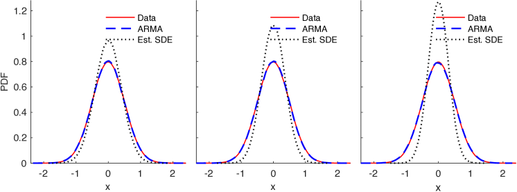
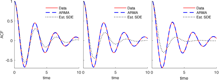
The long-term statistics, i.e., the empirical probability density function (PDF) and the autocorrelation function (ACF), are shown in Figure 1. For all the three values of $h$, the ARMA models reproduce the empirical PDF and ACF almost perfectly. The estimated SDEs miss the spread of the PDF and the amplitude of oscillation in the ACF, and these error become larger as $h$ increases.

Figure 1: Empirical PDF and ACF of the ARMA$(2,1)$ models and the estimated linear Langevin system (denoted by Est. SDE), in the cases $h=1/32$ (left column), $h=1/16$ (middle column) and $h=1/8$ (right column). The ARMA models reproduce the PDF and ACF almost perfectly, much better than the estimated SDEs.

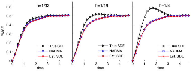
Next, we use an ensemble of trajectories to predict the motion of $x$. For each ensemble, we calculate the mean trajectory and compare it with the true trajectory from the data. We measure the performance of the prediction by computing the root-mean-square-error (RMSE) of a large number of ensembles as follows: take $N_{0}$ short pieces of data from the second half of the long trajectory, denoted by $\left\{\left(x_{\left(n_{i}+1\right)h},\dots,x_{\left(n_{i}+K\right)h}\right)\right\}_{i=1}^{N_{0}}$, where $n_{i}=Ki$. For each short piece of data $\left(x_{\left(n_{i}+1\right)h},\dots,x_{\left(n_{i}+K\right)h}\right)$, we generate $N_{ens}$ trajectories $\left\{\left(X_{1}^{i,j},\dots,X_{K}^{i,j}\right)\right\}_{j=1}^{N_{ens}}$ using a prediction system (i.e., the NARMA($p,q$), the estimated Langevin system, or the true Langevin system), starting all ensemble members from the same several-step initial condition $\left(x_{\left(n_{i}+1\right)h},\dots,x_{\left(n_{i}+m\right)h}\right)$, where $m=2\max\left\{p,q\right\}+1$. For the NARMA$\left(p,q\right)$ we start with $\xi_{1}=\cdots=\xi_{q}=0$. For the estimated Langevin system and the true Langevin system, we start with initial condition $\left(x_{\left(n_{i}+m\right)h},\hat{y}_{n_{i}}\right)$ with $\hat{y}_{n_{i}}=\frac{x_{\left(n_{i}+m\right)h}-x_{\left(n_{i}+m-1\right)h}}{h}$ and solve the equations using the Itô-Taylor scheme of order 2.0 with a time step $dt=1/64$ and record the trajectories every $h/dt$ steps to get the prediction trajectories $\left(X_{1}^{i,j},\dots,X_{K}^{i,j}\right)$.

We then calculate the mean trajectory for each ensemble, $\overline{X}_{k}^{i}=\frac{1}{N_{ens}}\sum_{j=1}^{N_{ens}}X_{k}^{i,j}$, $k=1,\dots,K$. The RMSE measures, in an average sense, the difference between the mean ensemble trajectory and the true data trajectory:

$$\mathrm{RMSE}(kh):=\left(\frac{1}{N_{0}}\sum_{i=1}^{N_{0}}\left|\overline{X}_{k}^{i}-x_{\left(n_{i}+k\right)h}\right|^{2}\right)^{1/2}.$$

The RMSE measures the accuracy of the mean ensemble prediction; $\mathrm{{RMSE}=0}$ corresponds to a perfect prediction, and small RMSEs are desired.

Figure 2: The linear Langevin system: RMSEs of $10^{4}$ forecasting ensembles with size $N_{ens}=20$, produced by the true system (denoted by True SDE), the system with estimated parameters (denoted by Est. SDE), and the ARMA model.

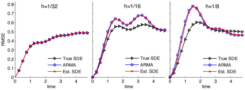
The computed RMSEs for $N_{0}=10^{4}$ ensembles with $N_{ens}=20$ are shown in Figure 2. The ARMA$\left(2,1\right)$ model reproduces almost exactly the RMSEs of the true system for all three observation step-sizes, while the estimated system has RMSEs deviating from that of the true system as $h$ increases. The estimated system has smaller RMSEs than the true system, because it underestimates the variance of the true process $x_{t}$ (that is, $\frac{\hat{\sigma}^{2}}{2\hat{\alpha}\hat{\gamma}}<\frac{\sigma^{2}}{2\alpha\gamma}$) and because the means of $x_{t}$ decay exponential to zero. The steady increase in RMSE, even for the true system, is entirely expected because the forecasting ensemble is driven by independent realizations of the forcing, as one cannot infer the white noise driving the system that originally generated the data.

4.2 The Kramers oscillator

We consider the Kramers equation in the following form

$$dx_{t} = y_{t}dt,$$

$$dy_{t} = (-\gamma y_{t}-\beta^{-2}x_{t}^{3}+x_{t})dt+\sigma dB_{t},$$ (4.2)

for which there are two potential wells located at $x=\pm\beta$.

In the continuous-time approach, the estimator $\hat{\theta}=\left(\hat{\gamma},\hat{\beta},\hat{\sigma}\right)$ is given by

$$\hat{\theta}=\arg\min_{\theta=\left(\gamma,\beta,\sigma\right)}\left[\sum_{n=1}^{N-3}\frac{3}{2}\frac{\left[\hat{y}_{n+2}-\hat{y}_{n+1}+h(\gamma\hat{y}_{n}+\beta^{-2}x_{n}^{3}-x_{n})\right]^{2}}{h\sigma^{2}}+\left(N-3\right)\log\sigma^{2}\right].$$ (4.3)

As for the linear Langevin system case, we begin by investigating the reliability of the estimators. A hundred simulated data sets are generated from the above Kramers oscillator with true parameters $\gamma=0.5,\beta=1/\sqrt{10},\sigma=1$, and with initial condition $x_{0}=y_{0}=1/2$ and integration time interval $[0,10^{4}]$. The estimators of $(\gamma,\beta,\sigma)$ are computed for each data set. Empirical mean and standard deviation of the estimators are shown in Table 3. We observe that the biases in the estimators increase as $h$ increases, in particular, the estimator of $\hat{\gamma}$ has a very large bias.

Table 3: Mean and standard deviation of the estimators of the parameters $(\gamma,\beta,\sigma)$ of the Kramers equation in the continuous-time approach, computed on 100 simulations.

Estimator	True value	$h=1/32$	$h=1/16$	$h=1/8$
$\hat{\gamma}$	$0.5$	$0.8726~{}(0.0063)$	$1.2049~{}\left(0.0057\right)$	$1.7003~{}\left(0.0088\right)$
$\hat{\beta}$	$0.3162$	$0.3501~{}\left(0.0007\right)$	$0.3662~{}\left(0.0007\right)$	$0.4225~{}\left(0.0009\right)$
$\hat{\sigma}$	$1$	$0.9964~{}\left(0.0014\right)$	$1.0132~{}\left(0.0027\right)$	$1.1150~{}\left(0.0065\right)$

Figure 3: RMSEs of model (M2), (M3), (M4) with ensemble size $N_{ens}=20$ in the case $h=1/8$. Models with $q=1$ have larger RMSEs than the models with $q=0$. In the case $q=0$, models (M2) and (M3) have almost the same RMSEs.

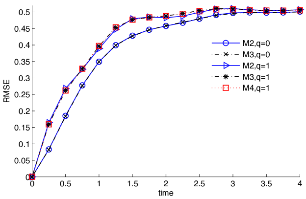
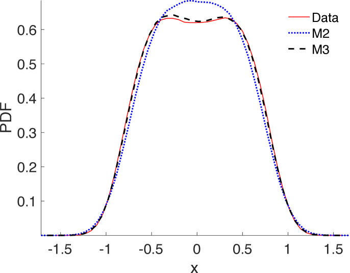
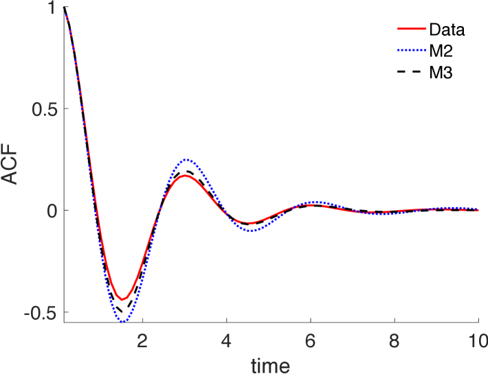
For the discrete-time approach, we have to select one of the four NARMA$\left(2,q\right)$ models, Model (M1)–(M4). We make the selection using data only from a single long trajectory (e.g. from the time interval $[0,T]$ with $T=2^{18}\approx 2\times 10^{5}$), and we use the first half of the data to estimate the parameters. We first estimate the parameters for each NARMA model with $q=0$ and $q=1$, using the conditional likelihood method described in Section 3.1. Then we make a selection by the criteria proposed in Section 3.1. First, we test numerical stability by running the model for a large time for different realizations of the noise sequence. We find that for our model, using the values of $h$ tested here, Model (M1) is often numerically unstable, so we do not compare it to the other schemes here. (In situations where the Euler scheme is more stable, e.g., for smaller values of $h$ or for other models, we would expect it to be useful as the basis of a NARMA approximation.) Next, we test the performance of each of the models (M2)–(M4). The RMSEs of models (M2), (M3) with $q=0$ and $q=1$ and Model (M4) with $q=1$ are shown in Figure 3. In the case $q=1$, the RMSEs for models (M2)–(M4) are very close, but they are larger than the RMSEs of models (M2) and (M3) with $q=0$. To make further selection between models (M2) and (M3) with $q=0$, we test their reproduction of the long-term statistics. Figure 4 shows that model (M3) reproduces the ACFs and PDFs better than model (M2), hence model (M3) with $q=0$ is selected.

Figure 4: Empirical PDFs and ACFs of the NARMA model (M2), (M3) and data in the case $h=1/8$. Model (M3) reproduces the ACF and PDF better than model (M2).

The mean and standard deviation of the estimated parameters of model (M3) with $q=0$ and 100 simulations are shown in Table 4. Unlike in the linear Langevin system case, we do not have a theoretical value for these parameters. However, note that when $h=1/32$, $\hat{a}_{1}$ and $\hat{a}_{2}$ are close to $2-\gamma h+0.5\gamma^{2}h^{2}=1.9845$ and $-(1-\gamma h+0.5\gamma^{2}h^{2})=-0.9845$ respectively, which are the coefficients in Eq. (3.3) from the Itô-Taylor scheme. This indicates that when $h$ is small, the NARMA model is close to the numerical scheme, because both the NARMA and the numerical scheme approximate the true system well. On the other hand, note that $\hat{\sigma}_{W}$ does not increase monotonically as $h$ increases. This clearly distinguishes the NARMA model from the numerical schemes.

Table 4: Mean and standard deviation of the estimators of the parameters of the NARMA model (M3) with $q=0$ in the discrete-time approach, computed from 100 simulations.

Estimator	$h=1/32$	$h=1/16$	$h=1/8$
$\hat{a}_{1}$	1.9906 (0.0004)	1.9829 (0.0007)	1.9696 (0.0014)
$-\hat{a}_{2}$	0.9896(0.0004)	0.9792 (0.0007)	0.9562 (0.0014)
$-\hat{b}_{1}$	0.3388 (0.1572)	0.6927 (0.0785)	1.2988 (0.0389)
$\hat{b}_{2}$	0.0300 (0.1572)	0.0864 (0.0785)	0.1462 (0.0386)
$\hat{b}_{3}$	0.0307 (0.1569)	0.0887 (0.0777)	0.1655 (0.0372)
$-\hat{\mu}~{}\left(\times 10^{-5}\right)$	0.0377 (0.0000)	0.1478 (0.0000)	0.5469 (0.0001)
$\hat{\sigma}_{W}$	0.0045 (0.0000)	0.1119 (0.0001)	0.0012 (0.0000)

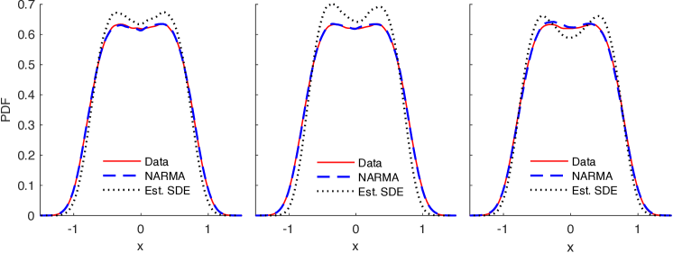
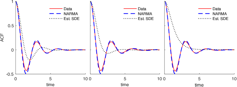
Next, we compare the performance of the NARMA model and the estimated Kramers system in reproducing long-term statistics and predicting short-term dynamics. The empirical PDFs and ACFs are shown in Figure 5. The NARMA models can reproduce the PDFs and ACFs equally well for three cases. The estimated Kramers system amplifies the depth of double wells in the PDFs, and it misses the oscillation of the ACFs.

Figure 5: Empirical PDFs and ACFs of the NARMA model (M3) with $q=0$ and the estimated Kramers system, in the cases $h=1/32$ (left column), $h=1/16$ (middle column) and $h=1/8$ (right column). These statistics are better reproduced by the NARMA models than by the estimated Kramers systems.

Results for RMSEs for $N_{0}=10^{4}$ ensembles with size $N_{ens}=20$ are shown in Figure 6. The NARMA model reproduces almost exactly the RMSEs of the true Kramers system for all three step-sizes, while the estimated Kramers system has increasing error as $h$ increases, due to the increasing biases in the estimators.

Figure 6: The Kramers system: RMSEs of $10^{4}$ forecasting ensembles with size $N_{ens}=20$, produced by the true Kramers system, the Kramers system with estimated parameters, and the NARMA model (M3) with $q=0$. The NARMA model has almost the same RMSEs as the true system for all the observation spacings, while the estimated system has larger RMSEs.

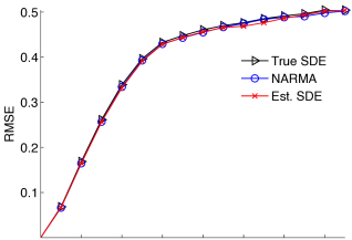
Finally, in Figure 7, we show some results using a much smaller observation spacing, $h=1/1024$. Figure 7(a) shows the estimated parameters, for both the continuous and discrete-time models. (Here, the discrete-time model is M2.) Consistent with the theory in [30], our parameter estimates for the continuous time model are close to their true values for this small value of $h$. Figure 7(b) compares the RMSE of the continuous-time and discrete-time models on the same forecasting task as before. The continuous-time approach now performs much better, essentially as well as the true model. Even in this regime, however, the discrete-time approach remains competitive.

Continuous-time model parameters $\hat{\gamma}$ $-\hat{\beta}$ $\hat{\sigma}$ 0.5163 0.3435 1.0006 Discrete-time model parameters $\hat{a}_{1}$ $-\hat{a}_{2}$ $-\hat{b}_{1}$ 1.9997 0.9997 0.0097 $-\hat{b}_{2}$ $-\hat{\mu}(\times 10^{-8})$ $\hat{\sigma_{W}}(\times 10^{-10})$ 0.0169 2.0388 6.2165
(a) Estimated parameter values		(b) $h=1/1024$

Figure 7: (a) Estimated parameters for the continuous-time and discrete-time models. (b) RMSEs of $10^{3}$ forecasting ensembles with size $N_{ens}=20$, produced by the true Kramers system (True SDE), the Kramers system with estimated parameters(Est. SDE), and the NARMA model (M2) with $q=0$. Since $h=1/1024$ is relatively small, the NARMA model and the estimated system have almost the same RMSEs as the true system. Here the data is generated by the Itô-Taylor solver with step size $dt=2^{-15}\approx 3\times 10^{-5}$, and data length is $N=2^{22}\approx 4\times 10^{6}$.

4.3 Criteria for structure design

Table 5: Consistency test. Values of the estimators in the NARMA models (M2) and (M3) with $q=0$. The data come from a long trajectory with observation spacing $h=1/32$. Here $N=2^{22}\approx 4\times 10^{6}$. As the length of data increases, the estimators of model (M2) have much smaller oscillation than the estimators of model (M3).

Data length	Model (M2)		Model (M3)
$(\times N)$	$-\hat{b}_{1}$	$-\hat{b}_{2}$	$-\hat{b}_{1}$	$\hat{b}_{2}$	$\hat{b}_{3}$
$1/8$	0.3090	0.3032	0.3622	0.0532	0.0563
$1/4$	0.3082	0.3049	0.3290	0.0208	0.0217
$1/2$	0.3088	0.3083	0.3956	0.0868	0.0845
$1$	0.3087	0.3054	0.3778	0.0691	0.0697

In the above structure selection between model (M2) and (M3), we followed the criterion of selecting the one that fits the long-term statistics best. However, there is another practical criterion, namely whether the estimators converge as the number of samples increases. This is important because the estimators should converge to the true values of the parameters if the model is correct, due to the consistency discussed in Section 3.1. Convergence can be tested by checking the oscillations of estimators as data length increases: if the oscillations are large, the estimators are likely not to converge, at least not quickly. Table 5 shows the estimators of the coefficients of the nonlinear terms in model (M2) and (M3), for different lengths of data. The estimators $\hat{b}_{1},\hat{b}_{2}$ and $\hat{b}_{3}$ of model (M3) are unlikely to be convergent, since they vary a lot for long data sets. On the contrary, the estimators $\hat{b}_{1}$ and $\hat{b}_{2}$ of model (M2) have much smaller oscillations, and hence they are likely to be convergent.

These convergence tests agree with the statistics of the estimators on 100 simulations in Tables 4 and 6. Table 4 shows that the standard deviations of the estimators $\hat{b}_{1},\hat{b}_{2}$ and $\hat{b}_{3}$ of model (M3) are reduced by half as $h$ doubles, which is the opposite of what is supposed to happen for an accurate model. On the contrary, Table 6 shows that the standard deviations of the parameters of model (M2) increase as $h$ doubles, as is supposed to happen for an accurate model.

In short, model (M3) reproduces better long-term statistics than model (M2), but the estimators of model (M2) are statistically better (e.g. in rate of convergence) than the estimators of model (M3). However, the two have almost the same prediction skill as shown in Figure 3, and both are much better than the continuous-time approach. It is unclear which model approximates the true process better, and it is likely that neither of them is optimal. Also, it is unclear which criterion is better for structure selection: fitting the long-term statistics or consistency of estimators. We leave these issues to be addressed in future work.

Table 6: Mean and standard deviation of the estimators of the parameters $(a_{1},a_{2},b_{1},b_{2},\mu,\sigma_{W})$ of the NARMA model (M2) with $q=0$ in the discrete-time approach, computed on 100 simulations.

Estimator	$h=1/32$	$h=1/16$	$h=1/8$
$\hat{a}_{1}$	1.9905 (0.0003)	1.9820 (0.0007)	1.9567 (0.0013)
$-\hat{a_{2}}$	0.9896 (0.0003)	0.9788 (0.0007)	0.9508 (0.0014)
$-\hat{b_{1}}$	0.3088 (0.0021)	0.6058 (0.0040)	1.1362 (0.0079)
$-\hat{b_{2}}$	0.3067 (0.0134)	0.5847 (0.0139)	0.9884 (0.0144)
$-\hat{\mu}~{}\left(\times 10^{-5}\right)$	0.0340 (0.0000)	0.1193 (0.0000)	0.2620 (0.0001)
$\hat{\sigma}_{W}$	0.0045 (0.0000)	0.1119 (0.0001)	0.0012 (0.0000)

5 Concluding discussion

We have compared a discrete-time approach and a continuous-time approach to the data-based stochastic parametrization of a dynamical system, in a situation where the data are known to have been generated by hypoelliptic stochastic system of a given form. In the continuous time case, we first estimated the coefficients in the given equations using the data, and then solved the resulting differential equations; in the discrete-time model, we chose structures with terms suggested by numerical algorithms for solving the equations of the given form, with coefficients estimated using the data.

As discussed in our earlier papers [8, 21], the discrete-time approach has several a priori advantages:

1. the inverse problem of estimating the parameters in a model from discrete data is in general better-posed in a discrete-time than in a continuous-time model. In particular, the discrete time representation is more tolerant of relatively large observation spacings.

2. once the discrete-time parametrization has been derived, it can be used directly in numerical computation, there is no need of further approximation. This is not a major issue in the present paper where the equations are relatively simple, but we expect it to grow in significance as the size of problems increases.

Our example validates the first of these points; the discrete-time approximations generally have better prediction skills than the continuous-time parametrization, especially when the observation spacing is relatively large. This was also the main source of error in the continuous models discussed in [8]; note that the method for parameter estimation in that earlier paper was completely different. Our discrete-time models also have better numerical properties, e.g., when all else is equal, they are more stable and produce more accurate long term statistics than their continuous-time counterparts.

We expect the advantages of the discrete-time approach to become more marked as one proceeds to analyze systems of growing complexity, particularly larger, more chaotic dynamical systems. A number of questions remain, first and foremost being the identification of effective structures; this is of course a special case of the difficulty in identifying effective bases in the statistical modeling of complex phenomena. In the present paper we introduced the idea of using terms derived from numerical approximations; different ideas were introduced in our earlier work [21]. More work is needed to generate general tools for structure determination.

Another challenge is that, even when one has derived a small number of potential structures, we currently do not have a systematic way to identify the most effective model. Thus, the selection of a suitable discrete-time model can be labor-intensive, especially compared to the continuous-time approach in situations where a parametric family containing the true model (or a good approximation thereof) is known. On the other hand, continuous-time approaches, in situations where no good family of models is known, would face similar difficulties.

Finally, another open question is whether discrete-time approaches generally produce more accurate predictions than continuous-time approaches for strongly chaotic systems. Previous work has suggested that the answer may be yes. We plan to address this question more systematically in future work.

Acknowledgments.

We would like to thank the anonymous referee and Dr. Robert Saye for helpful suggestions. KKL is supported in part by the National Science Foundation under grant DMS-1418775. AJC and FL are supported in part by the Director, Office of Science, Computational and Technology Research, U.S. Department of Energy, under Contract No. DE-AC02-05CH11231, and by the National Science Foundation under grant DMS-1419044.

Appendix A Solutions to the linear Langevin equation

Denoting

$$\mathbf{X}_{t}\mathbf{=}\left(\begin{array}[]{c}x_{t}\\ y_{t}\end{array}\right),\mathbf{A}=\left(\begin{array}[]{cc}0&1\\ -\alpha&-\gamma\end{array}\right),\text{ }\mathbf{e}=\left(\begin{array}[]{c}0\\ \sigma\end{array}\right),$$

we can write Eq. (3.4) as

$$d\mathbf{X}_{t}\mathbf{=AX}_{t}dt+\mathbf{e}dB_{t}.$$

Its solution is

$$\mathbf{X}_{t}=e^{\mathbf{A}t}\mathbf{X}_{0}+\int_{0}^{t}e^{\mathbf{A}(t-u)}\mathbf{e}dB_{u}.$$

The solution at discrete times can be written as

$$x_{\left(n+1\right)h} = a_{11}x_{nh}+a_{12}y_{nh}+W_{n+1,1},$$

$$y_{\left(n+1\right)h} = a_{21}x_{nh}+a_{22}y_{nh}+W_{n+1,2},$$

where $a_{ij}=\left(e^{\mathbf{A}h}\right)_{ij}$ for $i,j=1,2$, and

$$W_{n+1,i}=\sigma\int_{0}^{h}a_{i2}(u)dB\left(nh+u\right)$$ (A.1)

with $a_{i2}(u)=\left(e^{\mathbf{A}(h-u)}\right)_{i2}$ for $i=1,2$. Note that if $a_{12}\neq 0$, then from the first equation we get $y_{nh}=\left(x_{\left(n+1\right)h}-a_{11}x_{nh}-V_{n+1,1}\right)/a_{12}$. Substituting it into the second equation we obtain

$$x_{\left(n+2\right)h} = \left(a_{11}+a_{22}\right)x_{\left(n+1\right)h}+\left(a_{12}a_{21}-a_{11}a_{22}\right)x_{nh}$$

$$-a_{22}W_{n+1,1}+a_{12}W_{n+1,2}+W_{n+2,1}.$$

Combining with the fact that $a_{11}+a_{22}=\mathrm{trace}(e^{\mathbf{A}h})$ and $a_{12}a_{21}-a_{11}a_{22}=-e^{-\gamma h}$, we have

$$x_{\left(n+2\right)h}=\mathrm{trace}(e^{\mathbf{A}h})x_{\left(n+1\right)h}-e^{-\gamma h}x_{nh}-a_{22}W_{n+1,1}+W_{n+2,1}+a_{12}W_{n+1,2}.$$ (A.2)

Clearly, the process $\left\{x_{nh}\right\}$ is a centered Gaussian process, and its distribution is determined by its autocovariance function. Conditionally on $\mathbf{X}_{0}$, the distribution of $\mathbf{X}_{t}$ is $\mathcal{N}(e^{\mathbf{A}t}\mathbf{X}_{0},\mathbf{\Sigma}(t))$, where $\mathbf{\Sigma}(t):=\int_{0}^{t}e^{\mathbf{A}u}\mathbf{ee}^{T}e^{\mathbf{A}^{T}u}du$. Since $\alpha,\gamma>0$, the real parts of the eigenvalues of the $A$, denoted by $\lambda_{1}$ and $\lambda_{2}$, are negative. The stationary distribution is $\mathcal{N}(0,\mathbf{\Sigma}(\infty))$, where $\mathbf{\Sigma}(\infty)=\lim_{t\rightarrow\infty}\mathbf{\Sigma}(t)$. If $\mathbf{X}_{0}$ has distribution $\mathcal{N}(0,\mathbf{\Sigma}(\infty))$, then the process $\left(\mathbf{X}_{t}\right)$ is stationary, and so is the observed process $\left\{x_{nh}\right\}$. The following lemma computes the autocorrelation function of the stationary process $\left\{x_{nh}\right\}$.

Lemma A.1

Assume that the system $(\ref{OU})$ is stationary. Denote by $\left\{\gamma_{j}\right\}_{j=1}^{\infty}$ the autocovariance function of the stationary process $\left\{x_{nh}\right\}$, i.e. $\gamma_{j}:=\mathbb{E}[x_{kh}x_{(k+j)h}]$ for $j\geq 0$. Then $\gamma_{0}=\frac{\sigma^{2}}{2\alpha\gamma}$, and $\gamma_{j}$ can be represented as

$$\gamma_{j}=\gamma_{0}\times\left\{\begin{array}[]{cc}\frac{1}{\lambda_{1}-\lambda_{2}}(\lambda_{1}e^{\lambda_{2}jh}-\lambda_{2}e^{\lambda_{1}jh}),{}&\text{if }\gamma^{2}-4\alpha\neq 0;\\ e^{\lambda_{0}jh}(1-\lambda_{0}jh),&\text{if }\gamma^{2}-4\alpha=0\end{array}\right.$$

for all $j\geq 0$, where $\lambda_{1}$ and $\lambda_{2}$ are the different solutions to $\lambda^{2}+\gamma\lambda+\alpha=0$ when $\gamma^{2}-4\alpha\neq 0$, and $\lambda_{0}=-\gamma/2$.

Proof. Let $\mathbf{\Gamma}(j):=\mathbb{E}[\mathbf{X}_{kh}\mathbf{X}_{(k+j)h}^{T}]=\mathbf{\Sigma}(\infty)e^{\mathbf{A}^{T}jh}$ for $j\geq 0$. Note that $\gamma_{j}=\mathbf{\Gamma}_{11}(j)$, i.e., $\gamma_{j}$ is the first element of the matrix $\mathbf{\Gamma}(j)$. Then it follows that

$$\gamma_{0}=\mathbf{\Sigma}_{11}(\infty),~{}\gamma_{j}=\left(\mathbf{\Sigma}(\infty)e^{\mathbf{A}^{T}jh}\right)_{11}.$$

If $\gamma^{2}-4\alpha\neq 0$, then $\mathbf{A}$ has two different eigenvalues $\lambda_{1}$ and $\lambda_{2}$, and it can be written as

$$\mathbf{A}=\mathbf{Q\Lambda Q}^{-1}~{}\text{with}~{}\mathbf{Q=}\left(\begin{array}[]{cc}1&1\\ \lambda_{1}&\lambda_{2}\end{array}\right),\mathbf{\Lambda}=\left(\begin{array}[]{cc}\lambda_{1}&0\\ 0&\lambda_{2}\end{array}\right).$$

The covariance matrix $\mathbf{\Sigma}(\infty)$ can be computed as

$$\mathbf{\Sigma}(\infty)=\lim_{t\rightarrow\infty}\int_{0}^{t}\mathbf{Q}e^{\mathbf{\Lambda}u}\mathbf{Q}^{-1}\mathbf{ee}^{T}\mathbf{Q}^{-T}e^{\mathbf{\Lambda}^{T}u}\mathbf{Q}^{T}du=\sigma^{2}\left(\begin{array}[]{cc}\frac{1}{2ab}&0\\ 0&-\frac{1}{2b}\end{array}\right).$$ (A.3)

This gives $\gamma_{0}=\mathbf{\Sigma}_{11}(\infty)=\frac{\sigma^{2}}{2\gamma\alpha}$ and for $j>0$,

$$\gamma_{j}=\mathbf{\Sigma}_{11}(\infty)\left(e^{\mathbf{A}^{T}jh}\right)_{11}=\frac{1}{\lambda_{1}-\lambda_{2}}(\lambda_{1}e^{\lambda_{2}jh}-\lambda_{2}e^{\lambda_{1}jh})\gamma(0).$$

In the case $\gamma^{2}-4\alpha=0$, $\mathbf{A}$ has a single eigenvalue $\lambda_{0}=-\frac{\gamma}{2}$, and it can be transformed to a Jordan block

$$\mathbf{A=Q\Lambda Q}^{-1}~{}\text{with}~{}\mathbf{Q=}\left(\begin{array}[]{cc}1{}&0\\ \lambda_{0}{}&1\end{array}\right),\mathbf{\Lambda}=\left(\begin{array}[]{cc}\lambda_{0}{}&1\\ 0{}&\lambda_{0}\end{array}\right).$$

This leads to the same $\mathbf{\Sigma}(\infty)$ as in (A.3). Similarly, we have $\gamma_{0}=\frac{\sigma^{2}}{2\gamma\alpha}$ and

$$\gamma_{j}=\mathbf{\Sigma}_{11}(\infty)\left(e^{\mathbf{A}^{T}jh}\right)_{11}=e^{\lambda_{0}jh}(1-\lambda_{0}jh)\gamma_{0}.$$

 

Appendix B ARMA processes

We review the definition and computation of autocovariance function of ARMA processes in this subsection. For more details, we refer to [4, Section 3.3].

Definition B.1

The process $\left\{X_{n},n\in\mathbb{Z}\right\}$ is said to be an ARMA($p,q$) process if it is stationary process satisfying

$$X_{n}-\phi_{1}X_{n-1}-\cdots-\phi_{p}X_{n-p}=W_{n}+\theta_{1}W_{n-1}+\cdots+\theta_{q}W_{n-q},$$ (B.1)

for every $n$, where $\left\{W_{n}\right\}$ are i.i.d $\mathcal{N}(0,\sigma_{W}^{2})$, and if the polynomials $\phi(z):=1-\phi_{1}z-\dots-\phi_{p}z^{p}$ and $\theta(z):=1+\theta_{1}z+\dots+\theta_{q}z^{q}$ have no common factors. If $\left\{X_{n}-\mu\right\}$ is an ARMA($p,q$) process, then $\left\{X_{n}\right\}$ is said to be an ARMA($p,q$) process with mean $\mu$. The process is causal if $\phi(z)\neq 0$ for all $|z|\leq 1$. The process is invertible if $\theta(z)\neq 0$ for all $|z|\leq 1$.

The autocovariance function $\left\{\gamma(k)\right\}_{k=1}^{\infty}$ of an ARMA($p,q$) can be computed from the following difference equations, which are obtained by multiplying each side of (B.1) by $X_{n-k}$ and taking expectations,

$$\gamma(k)-\phi_{1}\gamma(k-1)-\dots-\phi_{p}\gamma(k-p) = \sigma_{W}^{2}\sum_{k\leq j\leq q}\theta_{j}\psi_{j-k},~{}~{}0\leq k<\max\{p,q+1\},$$ (B.2)

$$\gamma(k)-\phi_{1}\gamma(k-1)-\dots-\phi_{p}\gamma(k-p) = 0,~{}~{}~{}~{}~{}~{}~{}~{}k\geq\max\{p,q+1\},$$ (B.3)

where $\psi_{j}$ in (B.2) is computed as follows (letting $\theta_{0}:=1$ and $\theta_{j}=0$ if $j>q$)

$$\psi_{j}=\left\{\begin{array}[]{cc}{\theta_{j}+\sum_{0<k\leq j}\phi_{k}\psi_{j-k}},{}&\text{for }j<\max\{p,q+1\};\\ {\sum_{0<k\leq p}\phi_{k}\psi_{j-k}},&\text{for }j\geq\max\{p,q+1\}.\end{array}\right.$$

Denote $\left(\zeta_{i},i=1,\dots,k\right)$ the distinct zeros of $\phi(z):=1-\phi_{1}z-\cdots-\phi_{p}z^{p}$, and let $r_{i}$ be the multiplicity of $\zeta_{i}$ (hence $\sum_{i=1}^{k}r_{i}=p$). The general solution of the difference Eq. (B.3) is

$$\gamma(n)=\sum_{i=1}^{k}\sum_{j=0}^{r_{i}-1}\beta_{ij}n^{j}\zeta_{i}^{-n}\text{, for }n\geq\max\{p,q+1\}-p,$$ (B.4)

where the $p$ constants $\beta_{ij}$ (and hence the values of $\gamma(j)$ for $0\leq j<\max\{p,q+1\}-p$ ) are determined from (B.2).

Example B.2 (ARMA($2,0$))

. For an ARMA(2,0) process $X_{n}-\phi_{1}X_{n-1}-\phi_{2}X_{n-2}=W_{n}$, its autocovariance function is

$$\gamma(n)=\left\{\begin{array}[]{cc}{\beta_{1}\zeta_{1}^{-n}+\beta_{2}\zeta_{2}^{-n}},{}&\text{if }\phi_{1}^{2}+4\phi_{2}\neq 0;\\ {\left(\beta_{1}+\beta_{2}n\right)\zeta^{-n}},&\text{if }\phi_{1}^{2}+4\phi_{2}=0\end{array}\right.$$

for $n\geq 0$, where $\zeta_{1}$, $\zeta_{2}$ or $\zeta$ are the zeros of $\phi(z)=1-\phi_{1}z-\phi_{2}z^{2}$. The constants $\beta_{1}\,$and $\beta_{2}$ are computed from the equations

$$\gamma(0)-\phi_{1}\gamma(1)-\phi_{2}\gamma(2) = \sigma_{W}^{2},$$

$$\gamma(1)-\phi_{1}\gamma(0)-\phi_{2}\gamma(1) = 0.$$

Example B.3 (ARMA($2,1$))

. For an ARMA(2,1) process $X_{n}-\phi_{1}X_{n-1}-\phi_{2}X_{n-2}=W_{n}+\theta_{1}W_{n-1}$, we have $\psi_{0}=1,\psi_{1}=\phi_{1}$. Its autocovariance function is of the same form as that in $(\ref{gammaAR2})$, where the constants $\beta_{1}\,$and $\beta_{2}$ are computed from the equations

$$\gamma(0)-\phi_{1}\gamma(1)-\phi_{2}\gamma(2) = \sigma_{W}^{2}(1+\theta_{1}^{2}+\theta_{1}\phi_{1}),$$

$$\gamma(1)-\phi_{1}\gamma(0)-\phi_{2}\gamma(1) = \sigma_{W}^{2}\theta_{1}.$$

Appendix C Numerical schemes for hypoelliptic SDEs with additive noise

Here we briefly review the two numerical schemes, the Euler-Maruyama scheme and the Itô-Taylor scheme of strong order 2.0, for hypoelliptic systems with additive noise

$$dx = ydt,$$

$$dy = a(x,y)dt+\sigma dB_{t},$$

where $a:\mathbb{R}^{2}\to\mathbb{R}$ satisfies suitable conditions so that the system is ergodic.

In the following, the step size of all schemes is $h$, and $W_{n}=\sigma\sqrt{h}\xi_{n},~{}Z_{n}=\sigma h^{3/2}\left(\xi_{n}+\eta_{n}/\sqrt{3}\right)$, where $\left\{\xi_{n}\right\}$ and $\left\{\eta_{n}\right\}$ are two i.i.d sequences of $\mathcal{N}(0,1)$ random variables.
Euler-Maruyama (EM):

$$x_{n+1} = x_{n}+y_{n}h,$$ (C.1)

$$y_{n+1} = y_{n}+ha(x_{n},y_{n})+W_{n+1}.$$

Itô-Taylor scheme of strong order 2.0 (IT2):

$$x_{n+1} = x_{n}+hy_{n}+0.5h^{2}a\left(x_{n},y_{n}\right)+Z_{n+1},$$

$$y_{n+1} = y_{n}+ha\left(x_{n},y_{n}\right)+0.5h^{2}\left[a_{x}(x_{n},y_{n})y_{n}+\left(aa_{y}+0.5\sigma^{2}a_{yy}\right)(x_{n},y_{n})\right]$$

$$+W_{n+1}+a_{y}(x_{n},y_{n})Z_{n+1}+a_{yy}(x_{n},y_{n})\sigma^{2}\frac{h}{6}(W_{n+1}^{2}-h).$$

The Itô-Taylor scheme of order 2.0 can be derived as follows (see e.g. Kloeden and Platen [14, 18] ). The differential equation can be rewritten in the integral form:

$$x_{t} = x_{t_{0}}+\int_{t_{0}}^{t}y_{s}ds,$$

$$y_{t} = y_{t_{0}}+\int_{t_{0}}^{t}a(x_{s},y_{s})ds+\sigma\left(B_{t}-B_{t_{0}}\right).$$

We start from the Itô-Taylor expansion of $x:$

$$x_{t_{n+1}} = x_{t_{n}}+hy_{t_{n}}+\int_{t_{n}}^{t_{n+1}}\int_{t_{n}}^{t}a(x_{s},y_{s})dsdt+\sigma I_{10}^{n+1}$$

$$= x_{t_{n}}+hy_{t_{n}}+0.5h^{2}a(x_{t_{n}},y_{t_{n}})+\sigma I_{10}^{n+1}+O(h^{5/2}),$$

where $I_{10}^{n+1}:=\int_{t_{n}}^{t_{n+1}}\left(B_{t}-B_{t_{n}}\right)dt$. To get higher order scheme for $y$, we apply Itô’s chain rule to $a(x_{t},y_{t})$:

$$a\left(x_{t},y_{t}\right)=a\left(x_{s},y_{s}\right)+\int_{s}^{t}[a_{x}(x_{r},y_{r})y_{r}+(aa_{y}+0.5\sigma^{2}a_{yy})(x_{r},y_{r})]dr+\sigma\int_{s}^{t}a_{y}\left(x_{r},y_{r}\right)dB_{r}.$$

This leads to Itô-Taylor expansion for $y$ (up to the order 2.0):

$$y_{t_{n+1}} = y_{t_{n}}+\int_{t_{n}}^{t_{n+1}}a(x_{s},y_{s})ds+\sigma\left(B_{t_{n+1}}-B_{t_{n}}\right)$$

$$= y_{t_{n}}+ha\left(x_{t_{n}},y_{t_{n}}\right)+\sigma\left(B_{t_{n+1}}-B_{t_{n}}\right)+a_{y}(x_{t_{n}},y_{t_{n}})\sigma I_{10}^{n+1}+a_{yy}(x_{t_{n}},y_{t_{n}})\sigma^{2}I_{110}^{n+1}$$

$$+0.5h^{2}[a_{x}(x_{t_{n}},y_{t_{n}})y_{t_{n}}+(aa_{y}+0.5\sigma^{2}a_{yy})(x_{t_{n}},y_{t_{n}})]+O\left(h^{5/2}\right),$$

where $I_{110}^{n+1}=\int_{t_{n}}^{t_{n+1}}\int_{t_{n}}^{t}\left(B_{s}-B_{t_{n}}\right)dB_{s}dt$. Representing $\sigma\left(B_{t_{n+1}}-B_{t_{n}}\right)$, $\sigma I_{10}^{n+1}$ and $I_{110}^{n+1}$ by $W_{n+1}$, $Z_{n+1}$ and $\frac{h}{6}(W_{n+1}^{2}-h)$ respectively, we obtain the scheme (C).

References

- [1] E. B. Andersen. Asymptotic properties of conditional maximum-likelihood estimators. J. R. Stat. Soc. Series B, pages 283–301, 1970.
- [2] D. F. Anderson and J. C. Mattingly. A weak trapezoidal method for a class of stochastic differential equations. Commun. Math. Sci., 9(1), 2011.
- [3] L. Arnold and P. Imkeller. The Kramers oscillator revisited. In J. Freund and T. Pöschel, editors, Stochastic Processes in Physics, Chemistry, and Biology, volume 557 of Lecture Notes in Physics, page 280. Springer, Berlin, 2000.
- [4] P. Brockwell and R. Davis. Time series: theory and methods. Springer, New York, 2nd edition, 1991.
- [5] P. J. Brockwell. Continuous-time ARMA processes. Handbook of Statistics, 19:249–276, 2001.
- [6] P. J. Brockwell. Recent results in the theory and applications of CARMA processes. Ann. Inst. Stat. Math., 66(4):647–685, 2014.
- [7] P. J. Brockwell, R. Davis, and Y. Yang. Continuous-time Gaussian autoregression. Statistica Sinica, 17(1):63, 2007.
- [8] A. J. Chorin and F. Lu. Discrete approach to stochastic parametrization and dimension reduction in nonlinear dynamics. Proc. Natl. Acad. Sci. USA, 112(32):9804–9809, 2015.
- [9] S. Ditlevsen and M. Sørensen. Inference for observations of integrated diffusion processes. Scand. J. Statist., 31(3):417–429, 2004.
- [10] D. Frenkel and B. Smit. Understanding molecular simulation: from algorithms to applications, volume 1. Academic press, 2001.
- [11] A. Gloter. Parameter estimation for a discretely observed integrated diffusion process. Scand. J. Statist., 33(1):83–104, 2006.
- [12] G. A. Gottwald, D. Crommelin, and C. Franzke. Stochastic climate theory. In Nonlinear and Stochastic Climate Dynamics. Cambridge University Press, 2015.
- [13] J. D. Hamilton. Time Series Analysis. Princeton University Press, Princeton, NJ, 1994.
- [14] Y. Hu. Strong and weak order of time discretization schemes of stochastic differential equations. In Séminaire de Probabilités XXX, pages 218–227. Springer, 1996.
- [15] G. Hummer. Position-dependent diffusion coefficients and free energies from Bayesian analysis of equilibrium and replica molecular dynamics simulations. New J. Phys., 7(1):34, 2005.
- [16] A. C. Jensen. Statistical Inference for Partially Observed Diffusion Processes. PhD thesis, University of Copenhagen, Faculty of Science, Department of Mathematical Sciences, 2014.
- [17] R. H. Jones. Jones fitting a continuous time autoregressive to discrete data. In D. F. Findley, editor, Applied Time Series Analysis II, pages 651–682. Academic Press, New York, 1981.
- [18] P. E. Kloeden and E. Platen. Numerical Solution of Stochastic Differential Equations. Springer, Berlin, 3rd edition, 1999.
- [19] D. Kondrashov, M. D. Chekroun, and M. Ghil. Data-driven non-Markovian closure models. Physica D, 297:33–55, 2015.
- [20] H. A. Kramers. Brownian motion in a field of force and the diffusion model of chemical reactions. Physica, 7(4):284–304, 1940.
- [21] F. Lu, K. K. Lin, and A. J. Chorin. Data-based stochastic model reduction for the Kuramoto–Sivashinsky equation. arXiv:1509.09279, 2015.
- [22] A. J. Majda and J. Harlim. Physics constrained nonlinear regression models for time series. Nonlinearity, 26(1):201–217, 2013.
- [23] J. C. Mattingly, A. M. Stuart, and D. J. Higham. Ergodicity for SDEs and approximations: locally Lipschitz vector fields and degenerate noise. Stochastic Process. Appl., 101:185–232, 2002.
- [24] J. C. Mattingly, A. M. Stuart, and M. V. Tretyakov. Convergence of numerical time-averaging and stationary measures via Poisson equations. SIAM J. Numer. Anal., 48(2):552–577, 2010.
- [25] G. N. Milstein and M. V. Tretyakov. Computing ergodic limits for Langevin equations. Physica D: Nonlinear Phenomena, 229(1):81–95, 2007.
- [26] D. Nualart. The Malliavin calculus and related topics. Springer-Verlag, 2nd edition, 2006.
- [27] A. W. Phillips. The estimation of parameters in systems of stochastic differential equations. Biometrika, 46(1-2):67–76, 1959.
- [28] Y. Pokern, A. M. Stuart, and P. Wiberg. Parameter estimation for partially observed hypoelliptic diffusions. J. Roy. Statis. Soc. B, 71(1):49–73, 2009.
- [29] P. B.L.S. Rao. Statistical Inference for Diffusion Type Processes. Oxford University Press, 1999.
- [30] A. Samson and M. Thieullen. A contrast estimator for completely or partially observed hypoelliptic diffusion. Stochastic Process. Appl., 122(7):2521–2552, 2012.
- [31] L. Schimansky-Geier and H. Herzel. Positive Lyapunov exponents in the Kramers oscillator. J. Stat. Phys., 70(1-2):141–147, 1993.
- [32] H. Sørensen. Parametric inference for diffusion processes observed at discrete points in time: a survey. Int. Stat. Rev., 72(3):337–354, 2004.
- [33] M. Sørensen. Estimating functions for diffusion-type processes. In M. Kessler, A. Lindner, and M. Sørensen, editors, Statistical Methods for Stochastic Differential Equations. Oxford University Press, London, 2012.
- [34] D. Talay. Stochastic Hamiltonian systems: exponential convergence to the invariant measure, and discretization by the implicit Euler scheme. Markov Process. Related Fields, 8(2):163 – 198, 2002.