Testing the lognormality of the galaxy and weak lensing convergence distributions from Dark Energy Survey maps

Abstract

It is well known that the probability distribution function (PDF) of galaxy density contrast is approximately lognormal; whether the PDF of mass fluctuations derived from weak lensing convergence ($\kappa_{\rm{WL}}$) is lognormal is less well established. We derive PDFs of the galaxy and projected matter density distributions via the Counts in Cells (CiC) method. We use maps of galaxies and weak lensing convergence produced from the Dark Energy Survey (DES) Science Verification data over 139 deg². We test whether the underlying density contrast is well described by a lognormal distribution for the galaxies, the convergence and their joint PDF. We confirm that the galaxy density contrast distribution is well modeled by a lognormal PDF convolved with Poisson noise at angular scales from 10^′- 40^′(corresponding to physical scales of 3–10 Mpc). We note that as $\kappa_{\rm{WL}}$ is a weighted sum of the mass fluctuations along the line of sight, its PDF is expected to be only approximately lognormal. We find that the $\kappa_{\rm{WL}}$ distribution is well modeled by a lognormal PDF convolved with Gaussian shape noise at scales between 10^′and 20^′, with a best-fit $\chi^{2}$/DOF of 1.11 compared to 1.84 for a Gaussian model, corresponding to p-values 0.35 and 0.07 respectively, at a scale of 10^′. Above 20^′a simple Gaussian model is sufficient. The joint PDF is also reasonably fitted by a bivariate lognormal. As a consistency check we compare the variances derived from the lognormal modelling with those directly measured via CiC. Our methods are validated against maps from the MICE Grand Challenge N-body simulation.

1 Introduction

It was first noted by Hubble that the distribution of galaxies in angular cells on the celestial sphere is well approximated by a lognormal (Hubble, 1934). This has been confirmed observationally (Coles & Jones 1991, Wild et al. 2005) as well as in N-body simulations (Bernardeau & Kofman 1995, Bernardeau 1994, Kayo, Taruya & Suto 2001), which have shown that the underlying mass density field is expected to be lognormal.

Since the weak lensing convergence field along the line of sight is a weighted projection of the mass density contrast field, one might suspect that the lognormal distribution is a reasonable, if not exact, model of this too. This has been tested on numerical simulations and a lognormal PDF shown to be a reasonable model (Taruya, Hamana & Kayo 2002, Hilbert, Hartlap & Schneider 2011). Even better fits to the convergence PDF, particularly in the tails of the distribution, have been obtained by generalisations of a lognormal PDF (Das & Ostriker 2006, Takahashi et al. 2011, Joachimi, Taylor & Kiessling 2011).

The Dark Energy Survey (DES) (Dark Energy Survey Collaboration, 2005, 2015, 2016) presents an excellent opportunity to study both of these fields. DES was specifically conceived to produce cutting edge science from four different cosmological probes - large-scale structure, weak gravitational lensing, galaxy clusters and supernovae - using the same instrument. The full survey involves five years of observations, currently in progress. In this paper we focus on data produced during the pre-survey Science Verification (SV) series of observations.

This early data from DES allowed for the construction of two types of density fields. One is from luminous matter, i.e. galaxies of various types, $\delta_{g}$, which are biased tracers of the underlying dark matter field, $\delta_{m}$. The other uses the weak lensing of galaxy shapes to construct a convergence, or $\kappa$ map (Vikram et al., 2015; Chang et al., 2015) that is directly sensitive to the integrated dark matter field out to the lensed galaxies.

Both maps trace the underlying density distribution in the Universe. Galaxies are biased tracers of matter density, preferentially clustering in overdense regions. Galaxy density contrast can then be considered a biased local tracer of the density field.

Weak lensing convergence on the other hand responds directly to the underlying density field and is therefore unbiased. However gravitational deflection of light is a cumulative effect, sensitive to the integrated matter density along the line of sight from source galaxy to observer. The convergence field for a given galaxy source distribution therefore gives us information about the cumulative density field between observer and source, with the exact contribution of matter at different distances along the line of sight governed by the lensing efficiency function.

The purpose of the present study is to analyse the galaxy and mass maps from DES SV simultaneously, testing the two maps separately for log-normality, as well as analysing the joint distribution. To our knowledge this is the first time that the log-normality of the weak lensing convergence field alone has been tested using data rather than numerical simulation (Taruya et al., 2002), and the first time the joint distribution has been tested for log-normality.

The Counts in Cells (CiC) method (e.g. Hubble 1934; White 1979; Gaztanaga 1992; Szapudi 1997; Bernardeau et al. 2002) is a natural way to measure the individual and joint PDFs. The CiC technique splits up a particular data set into spatial cells, in two or three dimensions, and takes an aggregate of the available information inside each cell. Statistical variation between cells then provides information on the properties of that cosmological field.

DES observations are ideally suited to this sort of analysis. The fact that DES provides a joint galaxy survey and convergence map data set produced from the same observations makes it easier to ensure consistency between data and to control for systematics. The SV data we use were taken before the start of the full five year survey, covers 139 deg² to full survey depth and forms a test-bed for the kind of analyses planned on the final DES data. All of the analyses in this work are done first on galaxy and convergence maps from MICE simulations in order to test our methodology.

The outline of the paper is as follows. In section 2 we review the theory and formalism used. We describe the galaxy and weak lensing convergence maps from MICE simulations and DES used in section 3, and summarise our CiC method in section 4. In section 5 we validate our CiC method on MICE Grand Challenge N-body simulations, checking that we see the expected lognormality in MICE $\delta_{g}$ and the noise-free convergence. In section 6 we present lognormal fits to the individual DES galaxy and convergence field distributions as well as their joint distribution. We check the validity of the log-normal model by measuring the variance of the fields and comparing this to the variance derived under the assumption of log-normality. We discuss the results in 7, and in the Appendices we give the formalism used to calculate moments from CiC, test the impact of systematic effects, and confirm that assumptions we make in our method do not significantly affect our results.

2 Lognormal Modelling of cosmic fields

Lognormal distributions are very common in nature, from the sizes of clouds, pebbles on a beach, or crystals in icecream; the length of sentences or words in a conversation; to populations of bacteria (see Limpert, Stahel & Abbt 2001, Gaskell 2004 and references therein). Many of these examples involve multiplicative processes, of either merging or fragmentation. Any process that can be written as a product of terms will, if there are many terms, tend to a lognormal distribution. This is because if a process $X$ can be written as a product of independent terms, then $\rm{ln}(X)$ will be a sum of independent terms, and via the central limit theorem these will be normally distributed. So $\rm{ln}(X)$ is normally distributed, or, $X$ is lognormally distributed.

There are many examples of the hierarchical merging or fragmenting of structure leading to lognormal distributions, such as: the initial mass function of field stars, explained in terms of cloud fragmentation (Zinnecker, 1984); X-ray flux variations, suggesting lognormal distribution of emitting regions (Gaskell, 2004); luminosity functions of central galaxies, explained in terms of BCGs being formed by steps of mass adding/stripping (e.g. Taghizadeh-Popp, Heinis & Szalay 2012); and the angular momentum of disc galaxies (Marr, 2015).

In this paper we test the lognormality of the distribution of matter in the Universe via the galaxy density contrast field, $\delta_{g}$, and via the weak lensing convergence field, $\kappa_{\rm{WL}}$. Each approach has particular observational and astrophysical noise associated with it, which we discuss and propose models for in this section.

2.1 Galaxies

In the standard picture of gravitational instability, the primordial density fluctuations that are the precursor of all structure in the universe are assumed to be a random Gaussian field. Once they enter the non-linear regime, with finite rms fluctuations, their PDF must deviate from a Gaussian to avoid non-zero probabilities being attached to regions with negative densities (Fry, 1984). The exact form of the PDFs in this regime is not known but there are various phenomenological models that are fully specified statistically and satisfy the common sense requirement that the matter density, $\rho\geqslant 0$ (e.g. Saslaw & Hamilton 1984, Suto, Itoh & Inagaki 1990, Lahav et al. 1993, Gaztanaga & Yokoyama 1993; Suto 1993, Ueda & Yokoyama 1996).

One such model that is widely used is the lognormal. As well as being completely specified statistically and always having $\rho\geqslant 0$, it becomes arbitrarily close to Gaussian statistics at early times and has the advantage that it can be handled analytically. The merits of this model in a cosmological context are discussed extensively in Coles & Jones (1991). They explain possible motivations for using the lognormal model as: empirical; kinematic; an application of the central limit theorem (as described above); and importantly, simplicity. It is one of the few random fields for which interesting quantities such as its moments can be calculated analytically.

It should be noted that despite these compelling motivations to use a lognormal in the statistical treatment of density perturbations, it does have shortcomings. In particular, it is not uniquely specified by its moments; many distributions can lead to the same set of moments. It must then be the case that information is lost in going from a lognormal field to its moments, an effect quantified in Carron (2011). However, it remains a popular and useful tool in analysis of the mass density contrast field.

Galaxies are biased tracers of the mass density contrast field. The 1D log-normal distribution of galaxy density contrast $\delta_{g}$ = $(\rho-\bar{\rho})/\bar{\rho}$ is given by:

$$f(\delta_{g})\mathrm{d}\delta_{g}=\frac{1}{w\sqrt{2\pi}}exp\left(\frac{-x^{2}}{2w^{2}}\right)\mathrm{d}x$$ (1)

where $x=\mathrm{ln}(1+\delta_{g})+w^{2}/2$ and $w^{2}$ is the variance of the corresponding normal distribution $f[ln(1+\delta_{g})]$. The offset $w^{2}/2$ ensures that $\langle\delta_{g}\rangle=0$. The width $w$ is then the single free parameter of the 1D lognormal distribution.

If the lognormal distribution correctly describes the data, the variance of the overdensities will be related to the variance, $w$, of the underlying Gaussian distribution by

$$\langle\delta_{g}\delta_{g}\rangle=\mathrm{e}^{w^{2}}-1.$$ (2)

Due to the discrete nature of galaxies, shot noise is present. Assuming Poisson sampling of galaxies, the shot noise in the measurement of the distribution of galaxy overdensities can be accounted for by convolving the log-normal model with a Poisson distribution. The probability distribution function of the galaxy counts $N$ in a cell of given size is then given by:

$$P(N)=\int^{\infty}_{-1}\frac{\bar{N}^{N}(1+\delta_{g})^{N}}{N!}e^{-\bar{N}(1+\delta_{g})}f(\delta_{g})d\delta_{g}$$ (3)

This Poisson sampled lognormal distribution has been shown to be a good fit to different galaxy populations in Coles & Jones (1991), Blanton (2000) and Wild et al. (2005). In this work the smallest number of DES galaxies in a cell considered is around 300, so the shot noise term is important.

2.2 Weak Lensing Convergence

Various expressions for the convergence PDF have been proposed (Munshi & Jain, 2000; Valageas, 2000; Kainulainen & Marra, 2011). The lognormal model has the advantage - as in the case of the matter density contrast - of mathematical convenience, while offering the chance to extract more information than assuming a purely Gaussian model for the convergence field. Following a study that showed that a lognormal transformation of the matter density contrast increases the signal to noise (Neyrinck et al., 2009), Seo et al. (2011) performed an analogous study of the weak lensing convergence. They found that such a transform, when applied to the positively offset convergence, decorrelated angular frequencies and increased the signal-to-noise in the transformed power spectrum.

The convergence field along a line-of-sight can be expressed as a weighted projection of the mass density contrast field:

$$\kappa(\theta)=\int^{\chi_{\rm hor}}_{0}d\chi w(\chi)\delta[r(\chi)\theta,\chi],$$ (4)

where $\chi$ is the comoving distance, $\chi_{\rm hor}$ is the angular diameter distance to the horizon and $\delta[r(\chi)\theta,\chi]$ is the underlying matter density contrast field. $w(\chi)$ is a geometrical weight function that depends on the relative separations of sources, lens and the observer (see e.g. Mellier 1999; Bartelmann & Schneider 2001 for reviews). It takes the form

$$w(\chi)=\frac{3}{2}\left(\frac{H_{0}}{c}\right)^{2}\frac{\chi\Omega_{0}}{a(\chi)}\int_{\chi}^{\chi_{\rm hor}}d\chi^{\prime}n(\chi^{\prime})\frac{\chi^{\prime}-\chi}{\chi^{\prime}},$$ (5)

where $n(\chi)$ is the source galaxy distribution.

The distribution of $\kappa$ is not expected to be exactly lognormal, even if $\delta$ is, since $\kappa$ is a weighted projection of the mass density contrast field along line of sight. However, simulations have shown (Taruya et al., 2002) that the convergence field is well approximated by a lognormal outside the regime of extremely high $\kappa$. Hence we choose in this work to model the noise free $\kappa$ field distribution with a shifted lognormal

$$P(\kappa)=\begin{cases}\cfrac{\exp\Biggl{[}-\cfrac{(\textnormal{ln}(\kappa_{0}+\kappa)-\mu)^{2}}{2\sigma^{2}}\Biggr{]}}{\textnormal{ln}(\kappa_{0}+\kappa)\sqrt{2\pi}\sigma}&\text{for }\kappa>-\kappa_{0},\\ 0&\text{otherwise},\end{cases}$$ (6)

where the shift $\kappa_{0}=-\kappa_{min}$ and is called the ‘minimum convergence parameter’ (Hilbert et al., 2011). The lowest possible value of $\kappa$ is given by $-\kappa_{0}$ since the lognormal is only defined for a positive range. The mean is given by

$$\mu=\textnormal{ln}(\kappa_{0}+\langle\kappa\rangle)-\sigma^{2}/2$$ (7)

and the second moment

$$\langle\kappa\kappa\rangle=e^{(2\mu+\sigma^{2})}(e^{\sigma^{2}}-1).$$ (8)

The value assigned to $\kappa_{0}$ is a modelling choice that can be approached in several ways. The minimum measured value of $\kappa$ could be used, but this is a noisy quantity and should not be used unless one has access to many realisation of $\kappa$. Or, treating $\kappa$ analogously to $\delta_{g}$, we could consider a theoretical minimum corresponding to the convergence we would see, for a given source distribution, if the mass distribution was a pure void along the entire line of sight. For the MICE source distribution used in this work this value is $-0.050$, and for the DES source distribution it is $-0.053$. However simulations show that there are no empty lines of sight in a $\Lambda$CDM universe (Taruya et al., 2002; Vale & White, 2003; Hilbert et al., 2011). So we choose, where possible, to treat $\kappa_{0}$ as a free parameter and fit it jointly with the lognormal width.

Figure 1: Demonstration of the Gaussianity of the noise in DES weak lensing convergence, $\kappa$, at a smoothing scale of 20^′. Probability density distributions of the 100 realisations of the $\kappa$ map, in which shears were randomised, are shown in blue, with jackknife errors. A Gaussian PDF was fitted to each, with the mean of the best fitting PDFs shown in magenta. A Gaussian model is an excellent fit to the noise, with average goodness of fit $\chi^{2}/$DOF$=0.95\pm 0.73$.

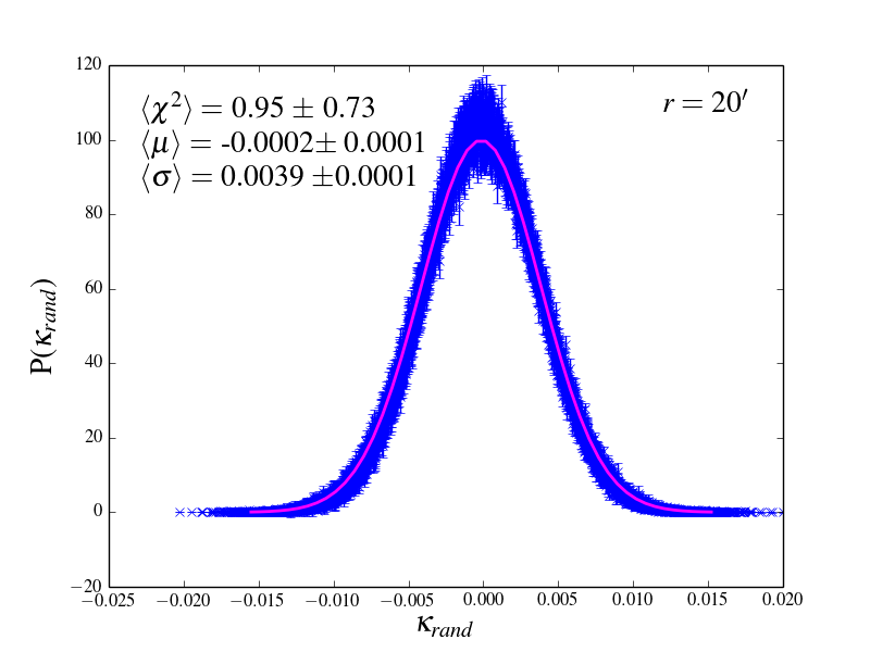
As for galaxies, we need to modify the lognormal to account for noise. The DES $\kappa$ map is constructed (see section 3.2) from measurements of shear, which is the change in the ellipticity of galaxies resulting from weak gravitational lensing. Since galaxies are intrinsically elliptical (i.e. in the absence of lensing), the observed shear is the sum of this intrinsic ellipticity and the shear caused by lensing. The variance of the intrinsic ellipticity, called shape noise, is the dominant source of noise in shear measurements, typically by a factor of more than an order of magnitude. An estimate of the shape noise in the DES $\kappa$ map is provided by the 100 noise realisations described in section 3.2.

To analyse the shape of the noise distribution we construct PDFs via CiC (as described in section 4) on each of the 100 maps. The resulting distributions appear Gaussian, as shown in figure 1, where the thick blue curve is made up of 100 superimposed noise distributions with jackknife error bars, and the magenta line shows the mean bestfit Gaussian PDF. A Gaussian model provides an excellent fit, with average goodness of fit over the 100 maps $\chi^{2}/dof=0.95\pm 0.73$.

We therefore propose that the 1D probability distribution for the weak lensing convergence field is then given by a convolution of a lognormal distribution with a noise contribution modelled as Gaussian:

$$f(\kappa)=\frac{1}{\sqrt{2\pi}\sigma_{n}}\int^{\infty}_{-\kappa_{0}}\exp\Big{[}-\frac{(\kappa^{\prime}-\kappa)^{2}}{2\sigma_{n}^{2}}\Big{]}P(\kappa^{\prime})\mathrm{d}\kappa^{\prime}$$ (9)

where $P(\kappa)$ is the noise free log-normal distribution given in equation 6, and $\sigma_{n}$ is the Gaussian width of the shape noise. In this work, $\sigma_{n}$ is determined from the 100 noise realisations.

2.3 Joint Galaxy and Weak Lensing Convergence Field

We can try to model the joint distribution of galaxy density contrast $\delta_{g}$ and weak lensing convergence $\kappa_{\rm{WL}}$ as a bivariate lognormal with PDF $f(\delta_{g},\kappa_{\rm{WL}})$. Following the notation used in Coles & Jones (1991); Wild et al. (2005), this is given by

$$f(\delta_{g},\kappa)=\frac{|V|^{-1/2}}{2\pi}\exp\left[-\frac{(\tilde{g}_{\delta}^{2}+\tilde{g}_{\kappa}^{2}-2r_{\text{LN}}\tilde{g}_{\delta}\tilde{g}_{\kappa})}{2(1-r^{2}_{\text{LN}})}\right],$$ (10)

where $g_{x}=\ln(x)-\left<\ln(x)\right>$, with $x=(1+\delta_{g})$ and $x=(1+\kappa/\kappa_{0})$ for the galaxy and convergence fields respectively, and $\tilde{g_{x}}=g_{x}/\omega_{x}$ where $\omega_{x}$ is the variance of the underlying Gaussian field $\ln(x)$.

The lognormal correlation coefficient $r_{\text{LN}}$ is given by

$$r_{\text{LN}}=\frac{\left<g_{\delta}g_{\kappa}\right>}{\omega_{\delta}\omega_{\kappa}}\equiv\frac{\omega^{2}_{\delta\kappa}}{\omega_{\delta}\omega_{\kappa}}$$ (11)

and $|V|$ is the determinant of the covariance matrix

$$V=\left(\begin{array}[]{cc}\omega^{2}_{\delta}&\omega^{2}_{\delta\kappa}\\ \omega^{2}_{\delta\kappa}&\omega^{2}_{\kappa}\end{array}\right).$$ (12)

Note that $r_{\text{LN}}$ and $V$ are defined in log-density space, and so $r_{\rm{LN}}$ is not the same as the (linear) Pearson correlation coefficient $\rho$. The conditional probability

$$f(\delta_{g}|\kappa) = \frac{f(\delta_{g},\kappa)}{f(\delta_{g})}$$ (13)

$$= \frac{w_{\delta}}{(2\pi|V|)^{1/2}}exp\Biggl{[}-\frac{(\tilde{g}_{\delta}-r_{\rm{LN}}\tilde{g}_{\kappa})^{2}}{2(1-r^{2}_{\rm{LN}})}\Biggr{]}.$$ (14)

Since $f(\delta_{g},\kappa)=f(\kappa)f(\delta_{g}|\kappa)$ we can combine equations 9 and 13 to give the joint probability distribution function $f(\delta_{g},\kappa)$. Including the convolutions with Poisson shot noise and Gaussian shape noise then gives

$$P(N,\kappa)=\int^{\infty}_{-1}\int^{\infty}_{-\kappa_{0}}\frac{1}{\sqrt{2\pi}\sigma_{n}}\exp\Big{[}-\frac{(\kappa^{\prime}-\kappa)^{2}}{2\sigma_{n}^{2}}\Big{]}f(\kappa)\\ \times\frac{\bar{N}^{N}(1+\delta_{g})^{N}}{N!}e^{-\bar{N}(1+\delta_{g})}f(\delta_{g}|\kappa)\mathrm{d}\delta_{g}\mathrm{d}\kappa^{\prime}$$ (15)

3 The Data

Figure 2: Redshift kernels of the observables considered in this paper: the galaxy redshift distribution of the DES Benchmark galaxy sample using the best-fit Skynet photo-z estimation (black line), and the lensing efficiency function of the sources used to make the DES $\kappa$ map (red line). Also shown is the redshift distribution of the source galaxies (shaded region). Each is shown with an arbitrary normalisation to make comparison easier.

This paper uses the DES Science Verfication (SV) galaxy and shape catalogues. The SV data were gathered between November 2012 and February 2013, shortly after DECam (Flaugher et al., 2015) commissioning, and before the beginning of the (five year) DES survey proper in August 2013. The operation of the camera, survey planning, data analysis and reduction were all tested in preparation for starting year one of DES itself. The SV goal was to reproduce the properties of the full five-year DES survey over a much smaller sky area.

Five optical filters ($grizY$) are used, with exposure times of 90 seconds for $griz$ and 45 seconds for $Y$. The final median depth in our region of interest, per band, was $g\sim 24.0$, $r\sim 23.9$, $i\sim 23.0$ and $z\sim 22.3$.

In total the SV data covered $\sim 250$ deg² at close to the nominal depth of the full DES survey. The observing footprint was divided into regions to maximise overlap with other surveys and with several small fields used for SNe searches.

In this paper we concentrate on a large contiguous region of $\sim$139 deg² called the SPT-E field due to its overlap with the South Pole Telescope CMB survey. This amount of contiguous data makes the SV SPT-E field a powerful data set in its own right, particularly for weak gravitational lensing where it rivals the full CFHTLenS (Erben et al., 2013) and is only slightly shallower.

3.1 DES Galaxy Sample

We use a particular subset of the DES SV galaxy catalogue known as the “Benchmark” sample (Crocce et al., 2015). First a catalogue of galaxies suitable for LSS analysis was constructed from the SV data and dubbed the “Gold” sample (Rykoff et al., 2016). Objects were included if detected in all five of the DES photometric bands. This covered $\sim$244 deg², restricted to $\textit{dec}>-61$ to avoid the Large Magellenic Cloud and R Doradus regions. In addition the Gold catalogue included masking of satellite trails and other artifacts, removal of regions where colors are severely affected by stray light and the application of additional stellar locus correction (Kelly et al., 2014).

From this Gold sample, the Benchmark sample was selected for cosmological analysis by imposing the additional conditions:

• $18.0<i<22.5$

• $0<g-r<3$, $0<r-i<2$ and $0<i-z<3$.

• wavg_spread_model $>$ 0.003 (star-galaxy separation)

• $60<ra<95$ and $-62<dec<-40$ (SPT-E),

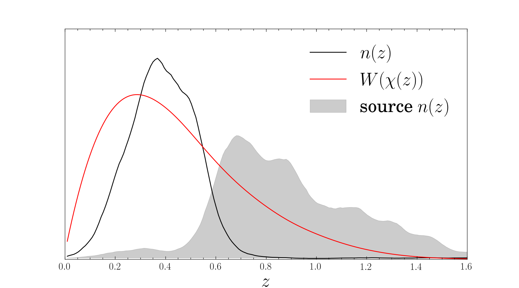
where $i$ refers to SExtractor’s MAG_AUTO quantity. The cuts on position restrict our analysis to the SPT-E region. The redshifts used in this paper come from the Skynet photo-z pipeline (Bonnett et al. 2015, Graff & Feroz 2013). The galaxy redshift distribution is shown in figure 2. The redshift range we use throughout this paper is $0.1<z<1.5$, chosen as in this region the galaxy redshift distribution overlaps with the lensing efficiency function used to make the DES $\kappa_{WL}$ map (see next section).

3.2 DES $\kappa$ Map

Shear measurement on DES SV galaxy images was performed with two independent pipelines: im3shape (Zuntz et al., 2013) and ngmix (Sheldon, 2014).

Extensive testing of both codes was carried out by the DES collaboration (see Jarvis et al. 2015 for details) and both pipelines passed all requirement tests for measurement of cosmic shear with the SV data set. A number of cuts were applied to both catalogues to remove stars, spurious detections, poor measurements and other effects that could bias shear measurement; these are also described in Jarvis et al. (2015).

Shear measurements for a given galaxy are headless vectors and the cosmic shear field is therefore a spin-2 quantity. To allow us to perform our CiC analysis on a scalar quantity we work with maps of weak lensing convergence, $\kappa$, a spin-0 field. This $\kappa$-reconstruction was performed using the Kaiser-Squires method (Kaiser & Squires, 1993), and the production and initial analysis of these $\kappa$ maps is described in detail in Vikram et al. (2015).

The Kaiser-Squires reconstruction method uses the relation of the Fourier transform of the observed shear, $\hat{\gamma}$, to that of the convergence, $\hat{\kappa}$,

$$\hat{\kappa}_{\ell}=D^{*}_{\ell}\hat{\gamma}_{\ell},$$ (16)

$$D_{\ell}=\frac{\ell_{1}^{2}-\ell_{2}^{2}+2i\ell_{1}\ell_{2}}{|\ell|^{2}},$$ (17)

where $\ell_{i}$ are the Fourier counterparts of the angular coordinates, $\theta_{i},i=1,2$. The inverse Fourier transform of equation 16 gives the convergence for the observed field in real space. In the absence of noise, systematics and masking, the convergence will be a real (spin-0) quantity. In reality these effects produce a non-zero imaginary component. It is most convenient to express the real part of the convergence map as a map of curl free E-modes, and the imaginary part as divergence free B-modes. The $\kappa$ maps have pixels of size 2^′. For use in this analysis the original flat sky $\kappa$ maps are transformed into HEALPix (Gorski et al., 2005) maps at resolution $N_{\text{side}}$=4096. This is done by dividing each pixel of the flat sky maps into 25 sub-pixels, and creating a HEALPix map by combining these sub-pixels. This procedure reduces inaccuracies in changing from one mapping system to another, and in tests gives the same angular power spectrum measurements as the flat sky map to well within the errors.

The source galaxy selection used to construct the $\kappa$ map used in this paper took galaxies with redshifts in the range $0.6<z<1.3$. The resulting redshift efficiency function is shown in figure 2. The lensing efficiency function peaks at $z\sim 0.3$, and our selection of galaxies at $0.1<z<0.5$ overlaps significantly with the range of redshifts to which the $\kappa$ map is sensitive.

In addition to the E-mode $\kappa$ map we make use of a number of other products made in the course of the DES mass-mapping analysis. A B-mode map was constructed by rotating the measured galaxy ellipticities by 45 degrees. The physical process of weak gravitational lensing does not induce B-modes in the convergence field so the B-mode map is a test of systematic effects in our observations, shear measurement and $\kappa$-reconstruction; it should be consistent with zero within our reconstruction noise. We will refer to the B-mode reconstructed map as $\kappa_{B}$.

In addition to the E- and B-mode maps we also make use of a series of noise-only realisations, made by taking the galaxy shape catalogue and rotating the measured shape of each galaxy by some random angle. $\kappa$ maps were then constructed from each randomised catalogue in the usual way. This has the effect of destroying all cosmological information in the resulting maps, while retaining the same noise properties as the data (because the distribution of galaxies on the sky and in redshift remains the same, as does the overall ellipticity distribution across the sample). 100 of these noise realisations were made and we use them to estimate the noise contribution in our measurement, as described in more detail in section 2.2.

Figure 3: Standard deviations of the $\kappa_{E}$, $\kappa_{B}$ signal (magenta) and 100 realisations in which the shears have been randomised (blue) at a cell size of 20^′. The random realisations of $\kappa_{E}$ give an estimate of the shape noise contribution to $\kappa_{E}$; this accounts for 80% of the $\kappa_{E}$ signal. The $\kappa_{B}$ signal is also a good estimate of the shape noise, with the standard deviation of the $\kappa_{B}$ signal agreeing with the rms standard deviation of $\kappa_{E}$ random realisations within 2%. These standard deviations are calculated via CiC and errors are from jackknife sampling.

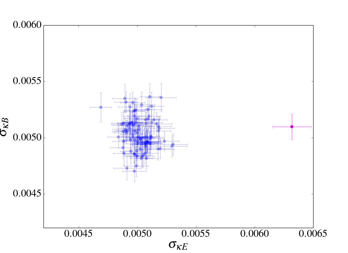
Fig. 3 shows the standard deviations of the $\kappa_{E}$, $\kappa_{B}$ signal (magenta) and 100 noise realisations (blue) for a cell size of 20^′. This shows that the shape noise (given by the random realisations of $\kappa_{E}$) accounts for 80% of the $\kappa_{E}$ signal, underlining the importance of accounting for shape noise in our modelling (as described in section 3.2). The shape noise dominates the signal most at small scales, accounting for 89% of the signal at 10^′ and dropping to 64% at 40^′. We can see that the $\kappa_{B}$ signal is also a good estimate of the shape noise, with the standard deviation of the $\kappa_{B}$ signal agreeing with the rms standard deviation of $\kappa_{E}$ random realisations within 2%. These standard deviations are calculated via CiC (see section 6.3 for a prescription for calculating moments from CiC) and errors are from jackknife sampling (see section 4).

3.3 MICE Simulations

We validate our measurement of CiC from DES SV data using a special set of mock catalogues produced from N-body simulations for the DES collaboration. These come from the Marenostrum Institut de Ciències de l’Espai Grand Challenges (MICE-GC hereafter) lightcone N-body simulation and associated halo catalogue.

These simulations have been used to produce mock galaxy catalogues for $\sim$200 million galaxies over 5000 deg² up to a redshift of $z=1.4$. There are also shear estimates for each galaxy made by ray-tracing through the N-body simulations. Every galaxy has a $\kappa_{\rm{WL}}$ value assigned from the integrated dark matter field.

The simulations are made with $4096^{3}$ particles of mass $2927M_{\odot}h^{-1}$ in a box of side 3072 $h^{-1}$Mpc. The MICE-GC has an assumed flat $\Lambda$CDM cosmology: $\Omega_{\rm m}=0.25$, $\Omega_{\rm b}=0.044$, $\Omega_{\Lambda}=0.75$, $\sigma_{8}=0.8$, $h=0.7$, $n_{s}=0.95$. The MICE-GC DES mocks approximately reproduce the magnitude limits of the DES survey and are complete down to apparent magnitude $i<22.0$ at $z=0.5$.

For use in this paper we have reduced the effective number densities in the mock galaxy and shear catalogues to reflect the statistics of the DES SV samples as well as normalising the redshift to reflect the distribution shown in Fig. 2. Each mock catalogue is projected onto a HEALPix map of $N_{side}=8192$, which is then degraded to match the resolution of our data maps where appropriate.

Figure 4: Distribution of MICE $\kappa_{\rm{WL}}$ at an angular scale of 10^′when DES-like shape noise is added. An estimate of the width of the shape noise distribution is obtained by fitting a Gaussian to the 100 random realisations of DES $\kappa_{\rm{WL}}$. A noise contribution drawn from a Gaussian of this width is added to MICE $\kappa_{\rm{WL}}$ at the level of the cells used to construct the CiC distribution. The darker, narrow histogram is that of the shape noise free MICE $\kappa_{\rm{WL}}$; the lighter histogram shows the distribution once the Gaussian shape noise is added; the black dashed line shows the observed distribution of DES $\kappa_{\rm{WL}}$. The Gaussian width of the DES shape noise estimate, $\sigma_{n}$ is 0.0099 at this scale, which is 89% of the width of the resulting noisy MICE $\kappa_{\rm{WL}}$ distribution.

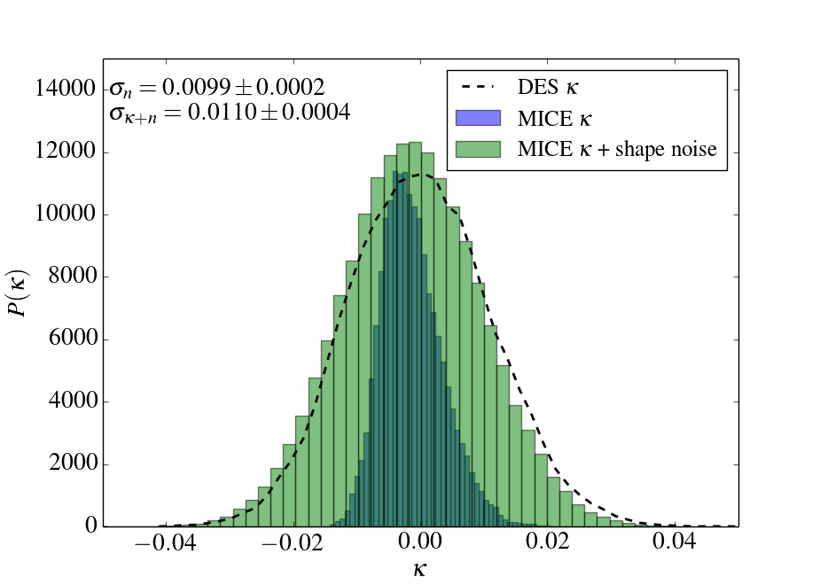
In order to be able to compare the distribution of DES $\kappa_{\rm{WL}}$ (which we know has a significant shape noise contribution) with simualtions, we create a second MICE $\kappa_{\rm{WL}}$ sample that has DES-like shape noise added. An estimate of the width of the shape noise distribution is obtained by fitting a Gaussian to the 100 random realisations of DES $\kappa_{\rm{WL}}$. A noise contribution drawn from a Gaussian of this width is added to MICE $\kappa_{\rm{WL}}$ at the level of the cells used to construct the CiC distribution.

Figure 4 shows the effect of adding shape noise to MICE $\kappa_{\rm{WL}}$ in this way at an angular scale of 10^′. The darker, narrow histogram is that of the shape noise free MICE $\kappa_{\rm{WL}}$; the lighter histogram shows the distribution once the Gaussian shape noise is added; and the black dashed line shows the distribution of DES $\kappa_{\rm{WL}}$. At a smoothing scale of 10 arcmin the Gaussian width of the DES shape noise estimate is 0.0099, which is 89% of the width of the resulting noisy MICE $\kappa_{\rm{WL}}$ distribution; this falls to 63% at 40^′.

4 Method

4.1 Constructing PDFs via Counts-in-Cells

The CiC approach is a relatively simple way to measure the distribution of galaxies in a survey, but it is a surprisingly powerful tool. A general CiC distribution for galaxies can be denoted by $f(N,V)$, the probability of finding $N$ galaxies in a volume of space $V$. This can be a 3D volume or, as is the case in this paper, a 2D area on the sky where we count over a population projected along the line of sight. Repeating this procedure with cells of varying radii, $r$, gives us the distribution $f_{r}(N)$, where the moments of $f_{r}(N)$ are related to the volume integrals of the correlation functions of our underlying observable (Peebles, 1980; Fry, 1985; Saslaw, 2000; Fry & Gaztanaga, 1994).

We perform our CiC analysis on the galaxy density contrast and weak lensing covergence maps with HEALPix pixelisation of resolution $N_{\text{side}}=4096$, which corresponds to an average pixel size of 0.9^′. For galaxies, to construct the PDF we sum the galaxy counts, $N$, inside 2D circular cells of fixed radius $r$ in the range 10–40^′. At the median redshift, $z=0.3$, of the sources considered this corresponds to physical scales of 3–10 Mpc. The smallest cells used are 10 times larger than the HEALPix pixels in order to minimise edge effects, and this also avoids any difference in counts across our survey area due to the changing geometry of the HEALPix pixels (see Appendix C for a discussion of this assumption). We chose to use randomly positioned circular cells rather than using the HEALPix pixels themselves as this allows us to repeat the analysis straightforwardly at any smoothing scale, rather than using only the fixed scales of HEALPix pixels. The criterion for accepting a cell is that 80% of its area should fall in unmasked regions (again see Appendix C for discussion of this choice). We want to use enough cells that all pixels in the map are covered at least once, and find that this is achieved when the total area of the cells is 20 times that of the survey. We use a coverage of 100 times the total area.

Histograms of the counts give us the distribution $f(N)$, and this procedure is repeated with cells of different radii to obtain the distribution $f_{r}(N)$. Double counting of pixels is accounted for by jackknife errors on the height of each bin in the resulting histogram of counts. We divide the survey area into 152 approximately equal area (1 deg²) jackknife patches. For a fixed set of randomly generated cells, and removing one patch at a time, we re-make the galaxy and convergence PDFs and re-calculate the statistics of interest in order to produce covariances.

We repeat our CiC analysis on the DES reconstructed $\kappa$ maps. The ‘count’ in each cell is now the average of the weak lensing convergence $\kappa$ in pixels contained in that cell.

In Appendix B we test the impact of spatially varying systematic effects on the DES $\delta_{g}$ and $\kappa_{\rm{WL}}$ CiC distributions.

It is straightforward to generalise our CiC method to more than one observable. We simply throw the same circles onto each map (using the same mask for each), allowing us to compare counts at the same position for different observables.

4.2 Fitting the PDFs

We fit the lognormal models described in section 2 to these distributions. For the MICE and DES galaxy density contrast distributions we fit a Poisson sampled lognormal using equation 3. For MICE $\kappa_{\rm{WL}}$, which has no shape noise, we fit a plain lognormal model (equation 6). For the $\kappa_{\rm{WL}}$ distributions which include shape noise (i.e. DES $\kappa_{\rm{WL}}$ and the MICE $\kappa_{\rm{WL}}$ to which we add shape noise), we use equation 9.

Figure 5: Correlation matrix of bin heights for a histogram of DES $\kappa_{\rm{WL}}$, at a smoothing scale of 10^′. Derived from jackknife sampling of the DES $\kappa_{\rm{WL}}$ map.

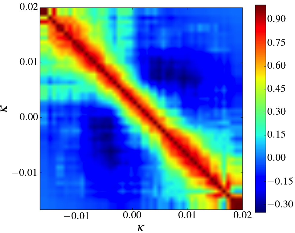
The histogram bins in $\delta_{g}$ or $\kappa_{\rm{WL}}$ are correlated. This is demonstrated in figure 5, which shows the correlation matrix of bin heights of DES $\kappa_{\rm{WL}}$ at a smoothing scale of 10^′. In fitting the lognormal model we take into account these correlations by minimising

$$\chi^{2}=(\vec{f}-\vec{d})\mathcal{C}^{-1}(\vec{f}-\vec{d})^{\prime}.$$ (18)

Here $f$ is the data vector of the lognormal fit at the bin centres, $d$ is the data vector of bin heights, and $\mathcal{C}$ is the covariance matrix. We remove weak eigenvectors of the covariance matrix via singular value decomposition.

5 Validating Methods on MICE

In this section we verify the methods used to test the lognormality of DES $\delta_{g}$ and $\kappa_{\rm{WL}}$ fields. After checking that the MICE $\delta_{g}$ field is lognormal as we would expect, we see if this is true of the noise-less convergence field.

To enable easier comparison with the DES $\kappa_{\rm{WL}}$ results we also look at the distribution of the simulation $\kappa_{\rm{WL}}$ for the MICE sample with number of galaxies and $n(z)$ matched to our DES sample, and with DES-like shape noise added. We then look at the joint distribution of $\delta_{g}$ and $\kappa_{\rm{WL}}$, for the cases with and without shape noise.

As an additional check of the validity of the lognormal model, we compare the second moments of the distributions as calculated via CiC with those derived under the assumption of lognormality.

5.1 Testing Lognormality of MICE Density and Convergence Fields

5.1.1 One-dimensional PDFs and log-normal fits

Figure 6: UPPER ROW: measured 1D PDF of MICE galaxies at a smoothing scales of 10, 15 and 30^′. The Poisson sampled lognormal fit (black) provides a better fit to the galaxy CiC distribution than the Gaussian (magenta) at a scale of 10^′. The distribution becomes increasingly Gaussian at larger scales. MIDDLE ROW: same as above but for the MICE $\kappa_{\rm{WL}}$ PDF. Again the lognormal provides a good fit at the smallest scale, with the $\kappa_{\rm{WL}}$ distribution becoming more Gaussian at larger scales. BOTTOM ROW: Fits to $\kappa_{\rm{WL}}$ using the sub-sample of MICE with DES-like galaxy density and $n(z)$, and to which DES-like shape noise has been added. This shape noise makes the distribution of $\kappa_{\rm{WL}}$ more Gaussian at all scales. All $\chi^{2}$ are per degree of freedom.

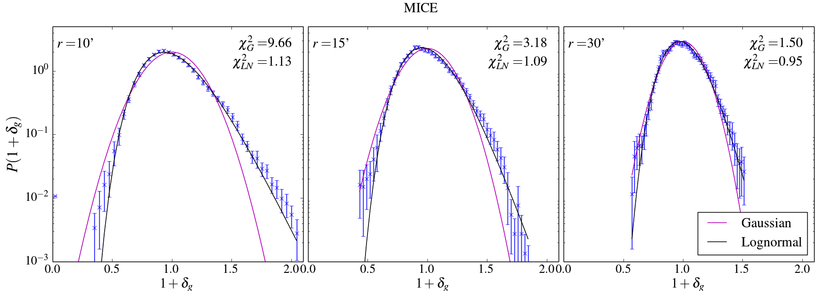
We first construct a simple histogram of $\delta_{g}$ from the CiC to estimate the 1D PDF of $\delta_{g}$. The histogram uses 50 bins and we calculate jackknife errors on the bin heights as described in the previous section. The result for cells of radius of 10, 15 and 30^′ is shown in the upper panel of Fig. 6. We fit a Poisson sampled lognormal distribution as described in eqn. 1 with $w$ as the single free parameter. The best-fit lognormal, which minimises $\chi^{2}$, is shown as a solid black line and the best fit Gaussian (magenta) is shown for comparison. At a cell size of 10^′ (corresponding to about 3 Mpc at the median redshift $z=0.3$) it is clear that the lognormal model fits the data better, reflecting the non-linear clustering at this scale. The counting of information inside a cell can be thought of as a form of smoothing where the cells form a top-hat filter with a fixed size. As the size of our cells increases we average information on increasingly large scales and lose sensitivity to the effects of non-linear clustering on small scales.

The lognormal distribution is designed to capture some of the information present as a result of non-linear evolution, so we would expect it to become less pronounced as the effective smoothing scale increases. This is indeed the case: at a cell radius of 10^′ the lognormal model is highly favoured, with a $\chi^{2}/DOF=1.13$, compared to 9.66 for the Gaussian. At a cell size 30^′ (corresponding to a physical scale of 8Mpc at the median redshift) the distribution has become much more Gaussian with best-fit $\chi^{2}$/DOF for the Gaussian model now 1.50. The lognormal model is still favoured at this scale, with best-fit $\chi^{2}$/DOF $=0.95$.

The result for the MICE $\kappa_{\rm{WL}}$ PDF is shown in the middle panel of fig. 6. Since there is no shape noise in the simulation we fit a plain lognormal, shown by the black line. As discussed in section 2.2, in order to fit a lognormal model to $\kappa_{\rm{WL}}$ one must assign a value to $\kappa_{0}$, the minimum convergence parameter in equation 6. At 10^′ we jointly fit $\kappa_{0}$ and the lognormal width in equation 6, finding best-fit $\kappa_{0}=0.021$. For larger scales we find that it is not possible to jointly constrain $\kappa_{0}$ and the width of the lognormal as they are degenerate. We therefore use the theoretically derived $\kappa_{0}=0.050$, described in section 2.2.

Since the convergence is the weighted sum of the mass fluctuations along the line of sight we expect it to be only approximately lognormal. At a smoothing scale of 10^′ the lognormal is a good fit, with $\chi^{2}$/DOF$=1.19$, and it is significantly preferred to the Gaussian model, which has a best-fit $\chi^{2}$/DOF$=14.43$. This lognormality of $\kappa_{\rm{WL}}$ at small scales is in line with Taruya et al. (2002) who found that a lognormal model was a good fit to simulated $\kappa_{\rm{WL}}$ at angular scales of 2 - 4^′. Increasing the cell radius above 10^′ removes the clear preference for the lognormal, and the lognormal and Gaussian models fit the data equally well at cell radii of 30^′. The fixed, theoretically derived $\kappa_{0}=0.050$ allows the lognormal model with a single free parameter to fit the distribution well at 15^′, but at larger cell radii this model does very slightly worse than the Guassian model. This suggests that this value of $k_{0}$ may not be a good estimate for the minimum $\kappa$ in the CiC PDF for larger cells. This makes sense as this $\kappa_{0}$ corresponds a pure void along the line of sight, which is a decreasingly likely observation as the cell radius increases.

The final row of figure 6 shows the distribution of $\kappa$ using the sub-sample of MICE with DES-like galaxy density and $n(z)$, and to which DES-like shape noise has been added, as described in section 3.3. The shape noise dominates the resulting distribution, particularly at smaller scales. The width of the distribution of shape noise is 74% of the width of the noisy $\kappa$ distribution at 40^′, and at 10^′ it accounts for 89%. We model the noisy $\kappa$ distribution with a lognormal convolved with Gaussian noise as described in section 2.2, using equation 9. Again we find that it is not possible to jointly constrain $\kappa_{0}$ and the width of the lognormal at scales above 10^′ as they are degenerate. We therefore use the theoretically derived $\kappa_{0}=0.049$. It can be seen from figure 6 that at all scales the shape noise makes the noisy $\kappa$ distribution much more Gaussian.

Despite the low signal to noise, at 10^′ the lognormal convolved with Gaussian noise provides a better fit than the simple Gaussian, with $\chi^{2}$/DOF$=1.06$ and 1.56 respectively. At scales larger than this the Gaussian model performs as well as the lognormal. As with the noise free convergence distribution, the theoretically derived $\kappa_{0}$ seems to be a less suitable choice at larger scales as the Gaussian model provides a better fit for scales above 30^′.

5.1.2 Joint galaxy-convergence distribution

In this sub-section we study the joint distribution of galaxy overdensities and weak lensing convergence and determine to what extent it can be described as a bivariate lognormal distribution. We look at joint distributions using both the full MICE sample, and the subsample with DES-like galaxy density and $n(z)$ and the addition of DES-like shape noise. As in the 1D case, the full sample with higher galaxy density allows us to better capture any lognormal behaviour, and the DES-like sample allows us to compare the results for DES data given in the next section with simulations.

We can make a simple quantitative estimate of the relative correlation of $\delta_{g}$ and $\kappa_{\rm{WL}}$ by calculating the Pearson product-moment correlation coefficient, $r$, for the joint PDF, where

$$\rho_{X,Y}=\frac{\textrm{Cov}(X,Y)}{\sigma_{X}\sigma_{Y}}=\frac{\left<(X-\bar{X})(Y-\bar{Y})\right>}{\sigma_{X}\sigma_{Y}}.$$ (19)

Figure 7: UPPER PANEL: Joint CiC distribution of weak lensing convergence and galaxy density contrast for MICE simulation at a smoothing scale of 15^′. The top right plot shows the bivariate lognormal fit to MICE simulations. Contours for the simulation are given by the solid blue lines, with dashed magenta contours for the fit. Also shown are the 1D PDFs for $1+\delta_{g}$ and $1+\hat{\kappa}_{WL}$ individually. PDFs are calculated via the CiC method with cells of radius 15^′. As in the rest of this paper, galaxies are selected over the redshift range $0.1<z<0.5$ and WL sources are restricted to the range $0.6<z<1.3$. This joint distribution has a Pearson correlation coefficient of $r=0.83$. LOWER PANEL: Same but with DES-like shape noise added to $\kappa_{\rm{WL}}$. The Pearson correlation coefficient drops to 0.45 with the addition of this shape noise.

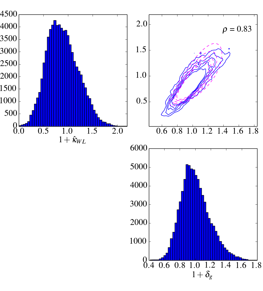
We begin with the joint distribution of $\delta_{g}$ and $\kappa_{WL}$ with no shape noise, which is shown in the upper panel of Fig. 7 for a smoothing scale of 15^′. The blue contours in the top right section of this plot show the joint PDF, and the dashed magenta contours show the bivariate lognormal fit. Since there is no shape noise in this case the bivariate fit is given by equation 15 but omitting the Gaussian convolution. We expect the correlation coefficient $\rho$ to be high (close to one) since the galaxies considered are responsible for the lensing. This is indeed what we see: the Pearson correlation coefficient is 0.81 at a smoothing scale 10^′ and 0.89 at 40^′. We do not see full correlation because the relevant window functions - the lensing efficiency function of the source sample and the galaxy redshift distribution of the galaxy sample - do not overlap precisely.

The lower panel of this figure shows the case where MICE $\kappa_{\rm{WL}}$ has had shape noise added. This noise reduces the correlation of the $\kappa_{\rm{WL}}$ with $\delta_{g}$, smearing out the joint distribution (shown on the top right of the figure) versus the shape noise free case. The Pearson correlation coefficient is reduced to 0.45.

5.2 Comparison of Moments

Figure 8: UPPER PANEL: comparison of second moments of MICE galaxy density contrast as a function of smoothing scale, directly measured via CiC and from lognormal and Gaussian fits to the CiC PDF. Blue data points show the ratio of the variance $\left<\delta_{g}^{2}\right>$ from our fits to the 1D lognormal distribution to that calculated directly from the CiC PDF; black data points show the same but for the Gaussian fit. Data points are offset slightly in scale for clarity. LOWER PANEL: same but for shape noise free MICE weak lensing convergence.

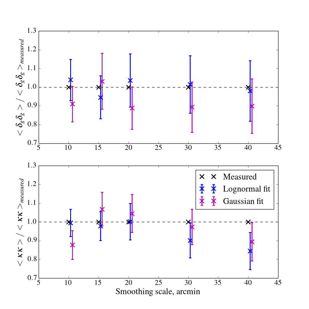
We can use the second moments to check the validity of the lognormal modelling by comparing the moments derived directly from the CiC with those derived by fitting a lognormal model to the CiC PDF. The second moments of the MICE galaxy and convergence fields $\langle\delta_{g}^{2}\rangle$ and $\langle\kappa^{2}\rangle$ can be calculated from the CiC (as described in Appendix A). The moments derived under lognormal modelling are given by equations 2 and 8.

First we calculate the variance of the MICE galaxy PDF, shown in the first panel of Fig. 8. Blue data points show the ratio of the variance $\left<\delta_{g}^{2}\right>$ from fitting a lognormal to the CiC PDF and that calculated directly from the CiC. Errors on $\left<\delta_{g}^{2}\right>$ directly from CiC are produced by jackknife sampling; errors on the $\left<\delta_{g}^{2}\right>$ derived from the lognormal fit are from the 1$\sigma$ width of the likelihood of the lognormal width.

The lognormal model gives a good estimate of the variance of the MICE galaxy density contrast distribution (with Poisson shot noise accounted for) at all scales. It gives a better estimate of the variance than a Gaussian model at all scales, and particularly at 10^′. The lognormal model also gives a good estimate of the variance of the weak lensing convergence distribution at scales up to 20^′. The poorer estimates at 30 and 40^′ are due to the fact that we fix $\kappa_{min}$ to the theory value at these scales.

These results suggest that within the ranges of scales discussed, the lognormal model can be used to estimate the two point statistics of both the galaxy density contrast and weak lensing convergence distributions to reasonable accuracy in these simulations.

6 Testing lognormality of DES density and convergence fields

Here we repeat the analysis of the previous section with DES galaxy and convergence maps, looking first distributions individually and then at their joint distribution.

6.1 One-dimensional PDFs and log-normal fits

Figure 9: UPPER ROW: measured 1D PDF of DES galaxies at a smoothing scales of 10, 15 and 30^′. At 10^′ the Poisson sampled log-normal fit (black) provides a much better fit than the Gaussian (magenta), demonstrating the log-normality of the galaxy CiC distribution at this scale. At larger scales the distribution becomes more Gaussian. LOWER ROW: same but for $\kappa_{\rm{WL}}$. Here the lognormal model includes Gaussian shape noise, which provides a good fit at all scales. Error bars on the counts PDFs are jackknife errors. All $\chi^{2}$ are per degree of freedom.

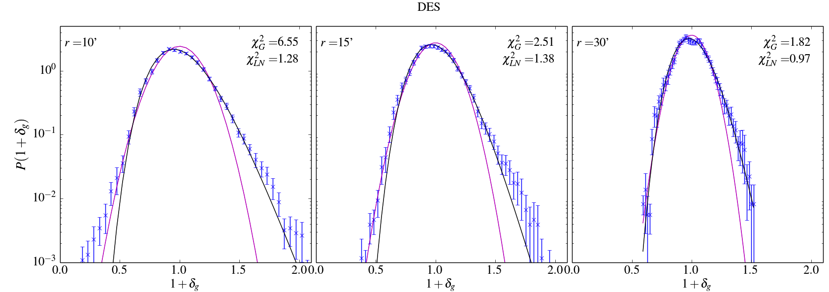
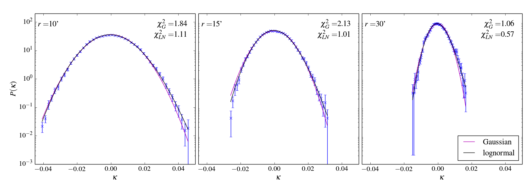
Fig. 9 shows 1D CiC PDFs for the DES galaxy density contrast (top row) and $\kappa_{\rm{WL}}$ (second row) fields for different cell radii. The lognormal fit is again shown in black, and for comparison a Gaussian fit is shown in magenta.

For the $\delta_{g}$ PDF at 10^′ the lognormal model is clearly favoured, with $\chi^{2}$/DOF$=1.28$ compared to 6.55 for the Gaussian model. This confirms the expected lognormal behaviour at non-linear scales, indicating that our CiC procedure is capturing non-linear clustering information beyond the Gaussian assumption at smaller radii. As in the simulations the $\delta_{g}$ PDFs clearly appear more Gaussian at larger cell radii, although the lognormal model still provides a better fit than the Gaussian even at 30^′, with $\chi^{2}$/DOF of 0.97 and 1.82 respectively.

$r$, arcmin	$\sigma$	$\chi^{2}_{G}$	$\chi^{2}_{LN}$	DOF	$\langle\delta_{g}\delta_{g}\rangle\times 10^{-2}$
10	0.184	72.05	14.08	11	$3.44\pm 0.30$
15	0.156	27.61	15.18	11	$2.46\pm 0.28$
20	0.146	21.48	12.36	12	$2.15\pm 0.29$
30	0.126	30.94	16.49	17	$1.60\pm 0.16$
40	0.122	22.88	18.48	22	$1.26\pm 0.17$

Table 1: Best-fit parameters and derived statistics from lognormal fits to CiC PDFs of DES galaxy density contrast, for varying cell radii. First first column gives the cell radius, and the second column is the width of the best fitting Poisson-sampled lognormal. The following columns are the minimum $\chi^{2}$ for Gaussian and Poisson sampled lognormal fits, and the number of degrees of freedom. The final column is the second moment of the best-fitting lognormal PDF, derived from the lognormal width, with $1\sigma$ errors given by the likelihood of the lognormal width.

The best-fit values of the free parameters of the lognormal fits to the DES galaxy density contrast distribution, the $\chi^{2}$, the number of degrees of freedom (DOF) and the second moment of the best-fit lognormal PDF are given in table 1, for smoothing scales of 10 - 40^′.

$r$, arcmin	$\kappa_{0}$	$\sigma$	$\chi^{2}_{G}$	$\chi^{2}_{LN}$	DOF	$\langle\kappa\kappa\rangle\times 10^{-5}$
10	0.021	0.235	18.41	11.10	10	$2.44\pm 0.45$
15	0.017	0.248	19.17	9.09	9	$1.59\pm 0.34$
20	0.016	0.238	10.92	4.63	10	$1.46\pm 0.29$
30	0.009	0.314	11.66	6.27	11	$0.84\pm 0.21$
40	0.008	0.300	14.82	8.58	13	$0.71\pm 0.19$

Table 2: Same as Table 1 but for DES weak lensing convergence. The lognormal fit accounts for shape noise, so the statistics quoted are for the de-noised $\kappa_{WL}$ distribution. The additional information given vs. Table 1 , in the second column, is the best-fit minimum convergence parameter $\kappa_{0}=-\kappa_{min}$.

The second row of Fig. 9 shows the DES $\kappa_{\rm{WL}}$ distribution. We find that it is possible to jointly constrain $\kappa_{0}$, the minimum convergence parameter in equation 6, and the width of the lognormal at all smoothing scales. The best-fit values of $\kappa_{0}$ as well as the lognormal width $\sigma$, best-fit $\chi^{2}$ and the second moment of the best-fit lognormal PDF are given in table 2. The best-fit $\kappa_{0}=0.021$ and $\sigma=0.235$ at cell radius 10^′ are in good agreement with the results from the MICE simulation at this scale, which are 0.023 and 0.226 respectively. Note that for larger scales we fix $\kappa_{0}$ at the theory value of 0.05 in the simulations, so would not expect close agreement of the best-fit lognormal width with that of the data at the these scales.

The $\kappa_{\rm{WL}}$ distribution appears quite Gaussian at all scales due to the Gaussian shape noise, the distribution of which has a width of 70-90% of the width of the $\kappa_{\rm{WL}}$ distribution. Despite this low signal to noise, as in the case of simulated $\kappa_{\rm{WL}}$, we find that the lognormal model with Gaussian shape noise (black line) provides a better fit than the simple Gaussian model (magenta line) at small scales. At 10^′ the lognormal model has $\chi^{2}=1.11$ and the Gaussian 1.84, corresponding to p-values of 0.35 for the lognormal model (i.e. within one $\sigma$) and 0.07 for the Gaussian model. At 15^′ the advantage of the lognormal model over the Gaussian is clear, with best-fit $\chi^{2}$/DOF of 1.01 and 2.13 respectively. At scales larger than this the Gaussian model provides a good fit with best-fit $\chi^{2}$/DOF of 1.09, 1.06 and 1.14 at 20, 30 and 40^′. The lognormal model is over-fitting the data at these scales, with $\chi^{2}$/DOF of 0.46, 0.57 and 0.66 at the same scales, so the Gaussian model is sufficient in this regime.

6.2 Joint galaxy-convergence distribution

Figure 10: Joint distribution of weak lensing convergence and galaxy density contrast for DES at smoothing scale 15^′. Upper right panel: Fit of bivariate lognormal to DES SV data. Contours for the data are given by the solid blue lines, with dashed magenta contours for the fit. Also shown are the individual 1D PDFs for $1+\delta_{g}$ and $1+\hat{\kappa}_{WL}$. DES Benchmark galaxies are used, selecting the redshift range $0.1<z<0.5$ and WL sources from the imshape catalogue are used over the range $0.6<z<1.3$. All redshifts are best-fits from the Skynet pipeline. PDFs are calculated via the CiC method with cells of radius 15^′. This joint distribution has a Pearson correlation coefficient of $r=0.45$.

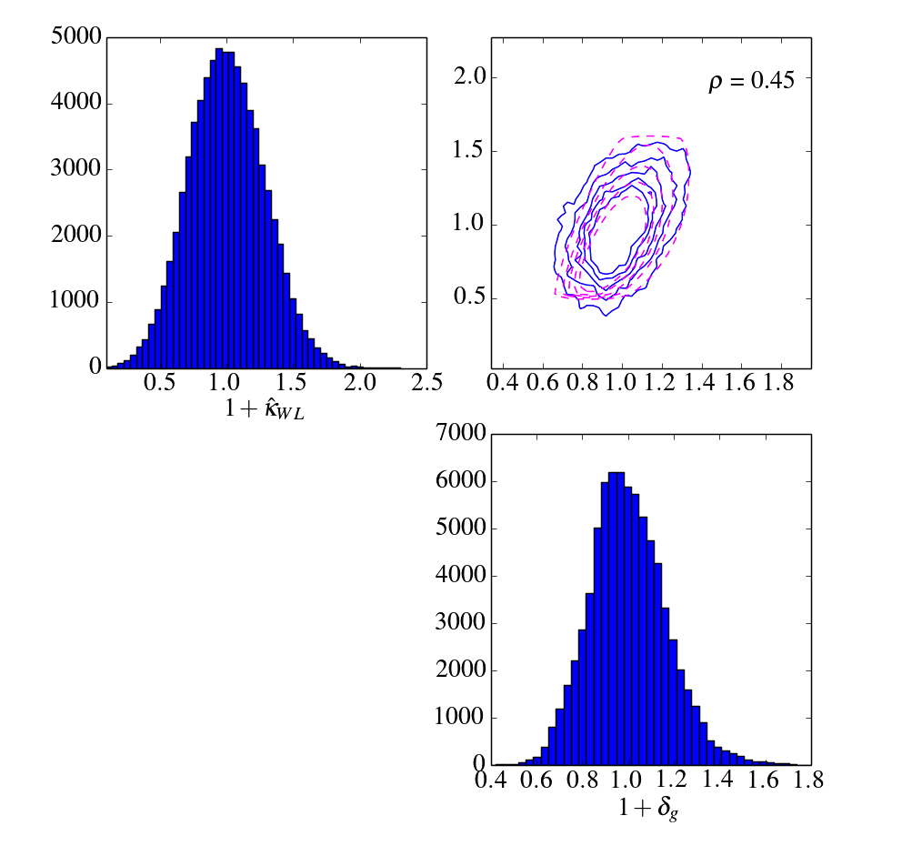
The joint distribution of DES galaxy density contrast and weak lensing convergence data at an angular scale of 15^′ is shown in the top right panel of fig. 10. The data are shown by the blue contours, and the bivariate fit is shown by the dashed magenta contours. The individual 1D PDFs for $1+\delta_{g}$ and $1+{\kappa/\kappa_{0}}$ are also shown.

Before we account for shot noise in the galaxies and shape noise in the convergence, the galaxy counts and $\kappa_{\rm{WL}}$ have a Pearson correlation coefficient of 0.45. This is in line with what we see in the MICE simulations once DES-like shape noise is added (bottom row of Fig. 7).

Once we account for these sources of noise, the correlation coefficient is 0.82, again in line with the noise-free MICE simulations, where the Pearson correlation coefficient was 0.83 (top row of Fig. 7).

6.3 Comparison of Second Moments

Figure 11: Same as figure 8, but for DES galaxies (upper panel) and convergence (lower panel).

$r$, arcmin	$\langle\delta_{g}\delta_{g}\rangle$	$\langle\kappa\kappa\rangle$	$\langle\ \kappa\kappa\rangle_{SN}$
10	$(3.70\pm 0.22)\times 10^{-2}$	$(2.52\pm 0.41)\times 10^{-5}$	$(1.00\pm 0.03)\times 10^{-4}$
15	$(2.76\pm 0.20)\times 10^{-2}$	$(1.69\pm 0.32)\times 10^{-5}$	$(4.68\pm 0.18)\times 10^{-5}$
20	$(2.26\pm 0.18)\times 10^{-2}$	$(1.39\pm 0.25)\times 10^{-5}$	$(2.60\pm 0.16)\times 10^{-5}$
30	$(1.65\pm 0.14)\times 10^{-2}$	$(9.84\pm 1.66)\times 10^{-6}$	$(1.18\pm 0.06)\times 10^{-5}$
40	$(1.38\pm 0.16)\times 10^{-2}$	$(8.40\pm 1.30)\times 10^{-6}$	$(6.75\pm 0.44)\times 10^{-6}$

Table 3: Second moments of DES galaxy density contrast and weak lensing convergence, as calculated by CiC, for different cell radii. Shot and shape noise have been accounted for, and these are the de-noised moments. The final column gives our estimate the shape noise of the weak lensing convergence. This is derived from the 100 realisations of the $\kappa_{\rm{WL}}$ map with randomised shears, which we find to agree with the second moment of the $\kappa_{\rm{WL}}$ B-mode within 2%.

In this section we check the validity of the lognormal model by comparing second moments derived from the log-normal assumption with those measured directly from the data.

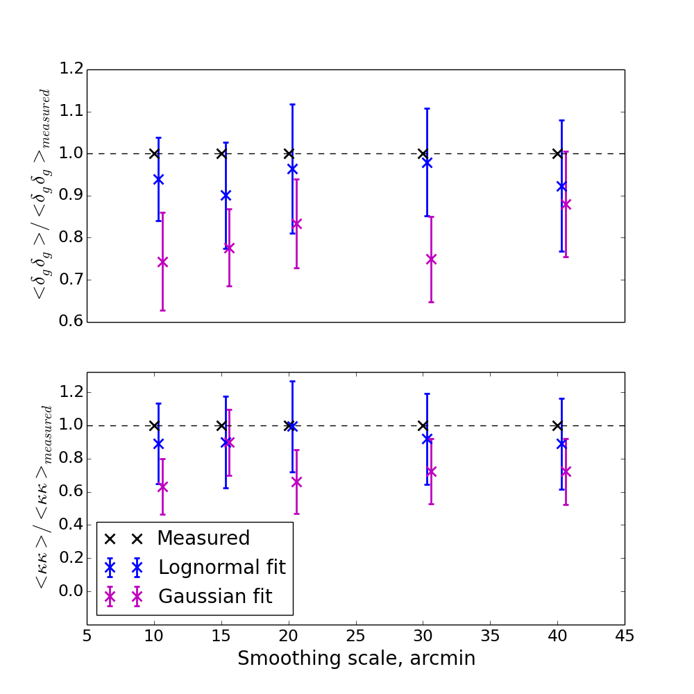
The variance of the DES galaxy PDF is shown in the first panel of Fig. 11. Blue data points show the ratio of the variance $\left<\delta_{g}^{2}\right>$ from our fits to the 1D lognormal distribution to that calculated directly from the CiC PDF. Errors on $\left<\kappa^{2}\right>$ directly from CiC are produced by jackknife sampling; errors on $\left<\kappa^{2}\right>$ derived from the lognormal fit are from the 1$\sigma$ width of the likelihood of the lognormal width. The second panels shows the same for DES $\kappa_{\rm{WL}}$. The lognormal model with appropriate noise contribution gives an estimate of the variance that is consistent with that calculated directly from the CiC, for both galaxies and $\kappa_{\rm{WL}}$, at all scales from 10 - 40^′.

For the galaxy density contrast distribution, the Gaussian model provides a less accurate estimate of the variance calculated directly from the CiC at all scales. For the convergence distribution the Gaussian model again gives variance estimates less accurate than the lognormal model at all scales.

For both galaxies and weak lensing convergence, the Gaussian and lognormal approaches underestimate the variance as compared to measuring it directly from the CiC. This is because in constructing the CiC PDF to which we fit the lognormal model, we bin the cell counts. We account for noise via singular value decomposition, and one of the things this removes is contributions to the fit from the outermost bins, which have very few cell counts. This makes the effective distribution narrower, with lower second moment, than if these noisy data points were included. In calculating the variance directly from the CiC (as described in Appendix A) this binning is not necessary and all cells, including those with the most extreme values of $\delta_{g}$ or $\kappa_{\rm{WL}}$, are included in the calculation, resulting in a larger variance in $\delta_{g}$ or $\kappa_{\rm{WL}}$. This effect is less stark in the MICE simulations where there are a greater number of galaxies than in the DES data, so fewer bins are discarded due to low counts of cells. This underestimation of the variance, however, is not significant within the errors.

7 Discussion

We have tested the lognormality of the DES galaxy density contrast and weak lensing convergence PDFs at angular scales of 10 - 40^′ (corresponding to physical scales of 3 - 10 Mpc at median redshift $z=0.3$). In the context of this work, estimating the CiC PDF is a way of quantifying the non-linear growth of mass and galaxy fluctuations, as well as the visual impression of comparing the $\kappa_{\rm{WL}}$ mass maps with the galaxy distribution on the same patch of the sky. It is also a test of systematics. Our main findings are as follows:

• In agreement with many earlier papers we find that the 1D DES galaxy PDF is well fitted by a lognormal model, taking into account Poisson shot noise, with best-fit $\chi^{2}$/DOF$=1.28$ vs. 6.55 for a Gaussian model at a scale of 10^′.

• In modelling the weak lensing convergence distribution it is important to account for shape noise since the width of this noise is a significant fraction (70-90%) of the width of the $\kappa_{\rm{WL}}$ signal. We find that the shape noise estimate derived from the 100 realisations of DES $\kappa_{\rm{WL}}$ in which the shears have been randomised agrees with that of the $\kappa_{B}$ mode within 2% at all scales from 10 to 40^′, and that the distribution of the shape noise can be well modeled by a Gaussian PDF. This allows us to model the $\kappa_{\rm{WL}}$ distribution with a lognormal convolved with Gaussian PDF. In future work it would be interesting to investigate the spatial correlation of this noise.

• The convergence field is not expected to be exactly lognormal even if the mass density contrast field is, as it is a weighted projection of the mass density field along the line of sight. We find however, in agreement with previous work on simulations, that the 1D $\kappa_{\rm{WL}}$ PDF is well fitted by a lognormal model, taking into account shape noise. This is the first such measurement on data. The best-fit $\chi^{2}$/DOF for the lognormal model is 1.11, compared to 1.84 for a Gaussian model, corresponding to p-values of 0.35 (i.e. within one $\sigma$) and 0.07 respectively. At scales above 15^′ the Gaussian model is a sufficient approximation.

• The bivariate ($\kappa_{\rm{WL}}$, $\delta_{g}$) PDF is also well fitted by a bivariate lognormal.

• De-noised second moments derived via the lognormal fit are consistent with variances derived directly from the data up to scales of 40^′, for both the DES galaxy density contrast and weak lensing convergence distributions.

This pilot study could be extended to much larger areas with weak lensing surveys such as the full DES (5000 deg²) survey, LSST (20,000 deg²) and Euclid (15,000 deg²). In this work we have tested the lognormality of the $\kappa_{\rm{WL}}$ PDF; with the higher signal/noise that future surveys will provide it might be possible to deduce from the observed $\kappa_{\rm{WL}}$ PDF whether or not the underlying matter density field is lognormal - essentially inverting equation 4.

In this work we have used the CiC to probe lognormality, but there is a wealth of information contained within it that could be exploited in future work. The CiC contains the full PDF so as well as the variance, higher order moments such as skewness and kurtosis can also be extracted.

The method used in this work, of constructing PDFs via CiC and cross correlating them, could be used to extract information on galaxy bias and to derive cosmological parameters. It could also be interesting to repeat this analysis using manipulations of the shear field than other $\kappa_{\rm{WL}}$ that avoid the reconstruction noise due to the Kaiser Squires method.

Quantifying $P(\kappa_{\rm{WL}})$ will be important for the emerging field of mass reconstruction using $\kappa_{\rm{WL}}$, since it is required as a prior input for this process. We have demonstrated that a lognormal model is a better choice than a Gaussian model at scales of 10 - 20^′. As well as the improved ability to capture non-linear behaviour versus a Gaussian model, the lognormal model still allows fast production of, for example, simulated realisations of the convergence field for testing, and covariance matrices.

Appendix A Measurement of moments from counts-in-cells

In section 5 we use the second moment, as calculated via CiC, as a check that the lognormal model accurately recovers the characteristics of the galaxy and $\kappa_{\rm{WL}}$ distributions. In this section we show how these are calculated for the galaxy and weak lensing convergence distributions, including how noise is accounted for.

Moments of a distribution are easily obtained via the CiC technique, with the $p^{th}$ central moment of the distribution of the number of objects $n$ at angular scale $\theta$ given by:

$$m_{p}(\theta)=\frac{1}{N(\theta)}\sum_{i=1}^{n_{c}(\theta)}\left(x_{i}(\theta)-\bar{x}\right)^{p}$$ (20)

where $N(\theta)$ is the number of cells of angular size $\theta$ used, $\bar{x}$ is the mean count of observable $x$ in a cell, and $x_{i}$ is the count in cell $i$. For the distribution of galaxies $x_{i}$ is the number of galaxies in a cell, and for the convergence $x_{i}$ is the average $\kappa$ within a cell.

The connected central moments $\mu_{p}(\theta)$ can be derived using the moment generating function (see §3.2.4 of Bernardeau et al. 2002 for a derivation and nice diagrammatic representation of the connected moments). The second connected moment is equal to the second central moment, $\mu_{2}=m_{2}$.

For the galaxy distribution, shot noise can be accounted for by assuming that galaxies form a Poisson sampling of the underlying matter density field:

$$P(\lambda)=\sum_{n=0}^{\infty}\lambda^{n}P(n).$$ (21)

Taylor expanding this around $\lambda=1$ gives $\langle n(n-1)...(n-p-1)\rangle=\bar{n}^{p}k_{p}$ where $k_{p}$ is the $p^{th}$ moment of the local density distribution. The ‘de-noised’ second moment is:

$$k_{2}=\mu_{2}-\bar{n},\\$$ (22)

where $\bar{n}$ is the mean number of galaxies in a cell. The area averaged correlations are then given by

$$\bar{w}_{p}=\frac{k_{p}}{\bar{n}_{p}},$$ (23)

For both the MICE and DES galaxy distributions, the second moment as calculated via CiC, with shot noise removed, is given by equations 20 - 23.

For $\kappa_{WL}$, since there is no need to model shot noise, $k_{2}=\mu_{2}$. The second moment for MICE $\kappa_{WL}$ is then given by equation 23. In the case of DES $\kappa$ we need to remove shape noise. The shape noise in the DES $\kappa_{WL}$ map is estimated from the 100 noise realisations, as discussed in section 3.2. Following Van Waerbeke et al. 2013, we assume the de-noised second moment of DES $\kappa_{WL}$ is then given by

$$\bar{w}_{2}=\bar{w}_{2,data}-\bar{w}_{2,noise}$$ (24)

where $\bar{w}_{2,noise}$ is given by equations 20 - 23 (with $k_{2}=\mu_{2}$), and $\bar{w}_{2,noise}$ is the mean of the second moments measured via CiC from each of the noise maps.

The second moment, estimated jointly from two distributions becomes

$$m_{2}(\theta) = \frac{1}{N(\theta)}\sum_{i=1}^{n_{c}(\theta)}\left(n_{\delta,i}(\theta)-\bar{n}_{\delta}\right)\left(\kappa_{i}(\theta)-\bar{\kappa}\right)$$ (25)

$$= \bar{n}_{\delta}\bar{n}_{\kappa}(\theta)\langle\delta_{i}(\theta)\kappa_{i}(\theta)\rangle$$ (26)

Appendix B Systematic Effects

Figure 12: UPPER ROW: PDF of DES galaxy number density at cell radii of 10, 15, 30^′ (blue data points) with jackknife errors. Coloured lines show PDFs with cuts for each systematic effect in turn. Lower panel shows the fractional difference between the full sample and those with systematics cuts, with errors shown by the grey shaded region. LOWER ROW: Same but for DES $\kappa_{WL}$.

We investigate the potential impact on our results of spatially varying systematics. The systematics we consider are varying the amount of air mass dependent on the distance of the observed field from the zenith, exposure time, magnitude limit, atmospheric seeing, and sky brightness. The values of these properties were mapped across the DES-SV area as described in Leistedt et al. (2015).

We compare PDFs of $\delta_{g}$ and $\kappa_{\rm{WL}}$ for the full samples used in this work versus when the areas worst-affected by these systematics are removed. We produce PDFs with the 20% of worst-affected pixels masked, for each systematic in turn.

Figure 12 shows the resulting distributions. The top row shows DES galaxy number density at cell radii of 10, 15, 30^′ (blue data points) with jackknife errors. Coloured lines show PDFs with cuts for each systematic effect in turn. The lower panel shows the fractional difference between the full sample and those with systematics cuts, with errors shown by the grey shaded region. The same for DES $\kappa_{\rm{WL}}$ is shown in the bottom row.

Here we can see that the PDFs of the cut data are broadly consistent with that of the full data, given the jackknife errors. For DES galaxies, for each systematic effect at least 95% of the bin heights after the cuts are made fall within the jackknife errors of the original distribution, and all are within 1.5 sigma of the original distribution. For DES $\kappa_{\rm{WL}}$, at least 93% of the new bin heights fall within the jackknife errors of the original distribution. All are within 1.9 sigma of the original data points. We can see that the effect of the systematics on the distribution increases with scale. Importantly PDFs of the cut $\kappa_{\rm{WL}}$ data at scales below 20^′, which is where we detect lognormality of $\kappa_{\rm{WL}}$, are completely consistent with the original distributions, i.e. all of the new bin heights fall within the errors of the original distribution. This simple test is reassuring and indicates that our lognormal fits to the DES $\delta_{g}$ and $\kappa_{\rm{WL}}$ distributions are not likely to be affected by these systematic effects.

Appendix C Tests of Sampling Methods

Figure 13: Second moment of MICE galaxy density contrast distribution as a function of scale as calculated via CiC, using underlying HEALPix maps with different resolutions. The HEALPix maps have nside (see main text) 512, 1024, 2048, 4096 corresponding to pixels of sizes shown by the solid circles. At scales approaching the pixel size edge effects are visible.

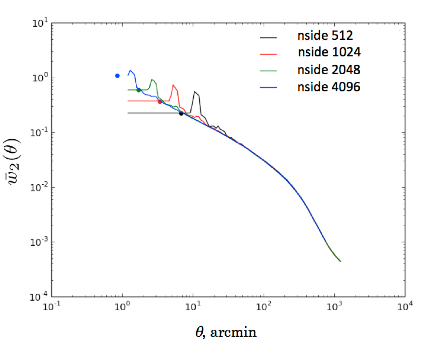
Our CiC analysis has made particular choices for cell size and distribution when accounting for the mask and creating the underlying HEALPix maps. In this Appendix we test each of these assumptions and demonstrate that the conclusions of our analysis are robust to our methodological choices.

HEALPix tessellations are made up of pixels with equal area, but not equal shape. Using circles that encompass several pixels will reduce the effect of the different pixel shapes, more so the larger the circles relative to the pixels. To check that the effect of varying shapes is effectively mitigated in this way we measure the area averaged 2-point correlation $\bar{w}_{2}(\theta)$ for DES galaxies at different HEALPix resolutions (512, 1024, 2048, and 4096). Figure 13 shows that when the cells size is close to the pixel size the correlation function is not smooth due to the effects of pixel shape. Once the cells are several times larger than the average pixel separation the correlation function becomes smooth, and the correlation functions based on the different HEALPix resolutions converge. This confirms that the method of using circular cells several times larger than the pixel resolution does not suffer from the effects of pixel shape, and that the underlying pixel resolution is not important as long as the minimum cell size considered is sufficiently large.

Figure 14: Left panel: Effect of the mask threshold (fraction of a cell that must be unmasked in order to be included in the analysis) on the resulting probability distribution of MICE galaxies. Middle Panel: Effect of this threshold on the second moment. Right panel: The fraction of the cells randomly thrown that are kept in the analysis, and, of those kept, the fraction of the data that comes from re-weighting these cells.

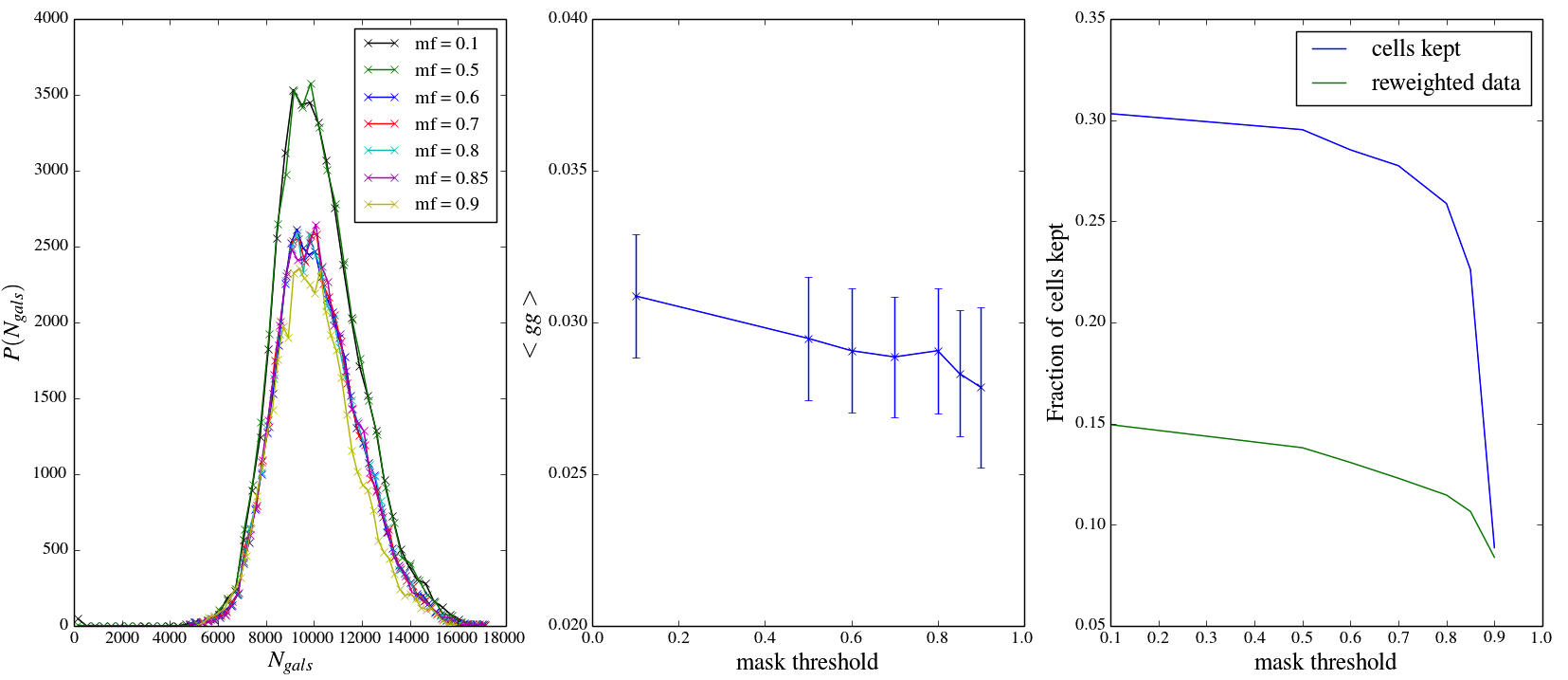
The other sampling assumption we test is the threshold at which we decide to discard a randomly positioned cell because too much of it is masked. If unmasked fraction of a randomly positioned cell is less than $f$, the counts are up-weighted to make it the equivalent of a whole cell. Here we explain the choice of $f=0.8$ used in this work.

The first panel of figure 14 shows the PDF of MICE galaxy counts for which the $f$ takes different values. For values of $f>0.5$ there is not much difference in the histograms by eye. The middle panel shows the variances of these different distributions, with errors produced by jackknife sampling. We find that the effect on the variance of changing $f$ is not significant within the errors.

If we chose a very high threshold, such as requiring 90% of a cell to be unmasked in order for it to be used, we would throw away a lot of cells landing near the edge of the survey and give greater statistical weight to areas away from the edges. If we set $f$ too low, so that cells with a large fraction of their area masked are kept, we will end up re-weighting a lot the data nearer the edges. So we would like to strike a balance between these two effects. From the right panel of figure 14 we can see than $f=0.8$ is the highest value that can be allowed before the number of cells we discard drops off significantly, and that at this value the fraction of data re-weighted is not too high (around 10%). Hence $f=0.8$ seems to be a sensible choice.

$[1]$ Astrophysics Group, Department of Physics and Astronomy, University College London, 132 Hampstead Road, London, NW1 2PS, United Kingdom
$[2]$ Department of Physics and Electronics, Rhodes University, PO Box 94, Grahamstown, 6140, South Africa
$[3]$ Department of Physics, ETH Zurich, Wolfgang-Pauli- Strasse 16, CH-8093 Zurich, Switzerland
$[4]$ Institute of Cosmology & Gravitation, University of Portsmouth, Portsmouth, PO1 3FX, UK
$[5]$Institut de Ciéncies de l’Espai (ICE, IEEC/CSIC), E-08193 Bellaterra (Barcelona), Spain
$[6]$ Istituto Nazionale di Astro sica - Osservatorio Astronomico di Brera, Via E. Bianchi 46, 23807 Merate, Italy
$[7]$ Department of Physics and Astronomy, University of Pennsylvania, Philadelphia, PA 19104, USA
$[8]$ Cerro Tololo Inter-American Observatory, National Optical Astronomy Observatory, Casilla 603, La Serena, Chile
$[9]$ Fermi National Accelerator Laboratory, P. O. Box 500, Batavia, IL 60510, USA
$[10]$ Department of Astrophysical Sciences, Princeton University, Peyton Hall, Princeton, NJ 08544, USA
$[11]$ CNRS, UMR 7095, Institut d’Astrophysique de Paris, F-75014, Paris, France
$[12]$ Sorbonne Universités, UPMC Univ Paris 06, UMR 7095, Institut d’Astrophysique de Paris, F-75014, Paris, France
$[13]$ Carnegie Observatories, 813 Santa Barbara St., Pasadena, CA 91101, USA
$[14]$ Kavli Institute for Particle Astrophysics & Cosmology, P. O. Box 2450, Stanford University, Stanford, CA 94305, US
$[15]$ SLAC National Accelerator Laboratory, Menlo Park, CA 94025, USA
$[16]$ Laboratório Interinstitucional de e-Astronomia - LIneA, Rua Gal. José Cristino 77, Rio de Janeiro, RJ - 20921-400, Brazil
$[17]$ Observatório Nacional, Rua Gal. José Cristino 77, Rio de Janeiro, RJ - 20921-400, Brazil
$[18]$ Department of Astronomy, University of Illinois, 1002 W. Green Street, Urbana, IL 61801, US
$[19]$ National Center for Supercomputing Applications, 1205 West Clark St., Urbana, IL 61801, USA
$[20]$ School of Physics and Astronomy, University of Southampton, Southampton, SO17 1BJ, UK
$[21]$ Excellence Cluster Universe, Boltzmannstr. 2, 85748 Garching, Germany
$[22]$ Faculty of Physics, Ludwig-Maximilians-Universität, Scheinerstr. 1, 81679 Munich, Germany
$[23]$ Jet Propulsion Laboratory, California Institute of Technology, 4800 Oak Grove Dr., Pasadena, CA 91109, USA
$[24]$ Department of Astronomy, University of Michigan, Ann Arbor, MI 48109, USA
$[25]$ Department of Physics, University of Michigan, Ann Arbor, MI 48109, USA
$[26]$ Kavli Institute for Cosmological Physics, University of Chicago, Chicago, IL 60637, USA
$[27]$ Center for Cosmology and Astro-Particle Physics, The Ohio State University, Columbus, OH 43210, USA
$[28]$ Department of Physics, The Ohio State University, Columbus, OH 43210, USA
$[29]$ Australian Astronomical Observatory, North Ryde, NSW 2113, Australia
$[30]$ Departamento de Física Matemática, Instituto de Física, Universidade de São Paulo, CP 66318, CEP 05314-970, São Paulo, SP, Brazil
$[31]$ Institució Catalana de Recerca i Estudis Avançats, E-08010 Barcelona, Spain
$[32]$ Institut de Física d’Altes Energies (IFAE), The Barcelona Institute of Science and Technology, Campus UAB, 08193 Bellaterra (Barcelona) Spain
$[33]$ Department of Physics and Astronomy, Pevensey Building, University of Sussex, Brighton, BN1 9QH, UK
$[34]$ Centro de Investigaciones Energéticas, Medioambientales y Tecnológicas (CIEMAT), Madrid, Spain
$[35]$ ICTP South American Institute for Fundamental Research
Instituto de Física Teórica, Universidade Estadual Paulista, São Paulo, Brazil

References

- Bartelmann & Schneider (2001) Bartelmann M., Schneider P., 2001, Physics Reports, 340, 291
- Bernardeau (1994) Bernardeau F., 1994, Astronomy and Astrophysics, 291, 24
- Bernardeau & Kofman (1995) Bernardeau F., Kofman L., 1995, The Astrophysical Journal, 443, 479
- Bernardeau et al. (2002) Bernardeau F., Colombi S., Gaztañaga E., Scoccimarro R., 2002, Phys. Rep., 367, 1
- Blanton (2000) Blanton M., 2000, The Astrophysical Journal, 544, 63
- Bonnett et al. (2015) Bonnett C., et al., 2015, eprint arXiv:1507.05909
- Carron (2011) Carron J., 2011, The Astrophysical Journal, 738, 86
- Chang et al. (2015) Chang C., et al., 2015, Physical Review Letters, 115, 051301
- Coles & Jones (1991) Coles P., Jones B., 1991, Monthly Notices of the Royal Astronomical Society, 248, 1
- Crocce et al. (2015) Crocce M., et al., 2015, Monthly Notices of the Royal Astronomical Society, 455, 4301
- Dark Energy Survey Collaboration (2005) Dark Energy Survey Collaboration 2005, eprint arXiv:astro-ph/0510346, p. 42
- Dark Energy Survey Collaboration (2015) Dark Energy Survey Collaboration 2015, eprint arXiv:1507.05552, p. 20
- Dark Energy Survey Collaboration (2016) Dark Energy Survey Collaboration 2016, Monthly Notices of the Royal Astronomical Society, pp stw641, arXiv:1601.00329v2
- Das & Ostriker (2006) Das S., Ostriker J. P., 2006, The Astrophysical Journal, 645, 1
- Erben et al. (2013) Erben T., et al., 2013, Monthly Notices of the Royal Astronomical Society, 433, 2545
- Flaugher et al. (2015) Flaugher B., et al., 2015, The Astronomical Journal, 150, 150
- Fry (1984) Fry J. N., 1984, The Astrophysical Journal, 279, 499
- Fry (1985) Fry J. N., 1985, The Astrophysical Journal, 289, 10
- Fry & Gaztanaga (1994) Fry J. N., Gaztanaga E., 1994, The Astrophysical Journal, 425, 1
- Gaskell (2004) Gaskell C. M., 2004, The Astrophysical Journal, 612, L21
- Gaztanaga (1992) Gaztanaga E., 1992, The Astrophysical Journal, 398, L17
- Gaztanaga & Yokoyama (1993) Gaztanaga E., Yokoyama J., 1993, The Astrophysical Journal, 403, 450
- Gorski et al. (2005) Gorski K. M., Hivon E., Banday A. J., Wandelt B. D., Hansen F. K., Reinecke M., Bartelmann M., 2005, The Astrophysical Journal, 622, 759
- Graff & Feroz (2013) Graff P., Feroz F., 2013, Astrophysics Source Code Library
- Hilbert et al. (2011) Hilbert S., Hartlap J., Schneider P., 2011, Astronomy & Astrophysics, 536, A85
- Hubble (1934) Hubble E., 1934, The Astrophysical Journal, 79, 8
- Jarvis et al. (2015) Jarvis M., et al., 2015, eprint arXiv:1507.05603
- Joachimi et al. (2011) Joachimi B., Taylor A. N., Kiessling A., 2011, Spectrum, 22, 27
- Kainulainen & Marra (2011) Kainulainen K., Marra V., 2011, Physical Review D - Particles, Fields, Gravitation and Cosmology, 84
- Kaiser & Squires (1993) Kaiser N., Squires G., 1993, The Astrophysical Journal, 404, 441
- Kayo et al. (2001) Kayo I., Taruya A., Suto Y., 2001, The Astrophysical Journal, 561, 22
- Kelly et al. (2014) Kelly P. L., et al., 2014, Monthly Notices of the Royal Astronomical Society, 439, 28
- Lahav et al. (1993) Lahav O., Itoh M., Inagaki S., Suto Y., 1993, The Astrophysical Journal, 402, 387
- Leistedt et al. (2015) Leistedt B., et al., 2015, eprint arXiv:1507.05647, p. 13
- Limpert et al. (2001) Limpert E., Stahel W. A., Abbt M., 2001, BioScience, 51, 341
- Marr (2015) Marr J. H., 2015, Monthly Notices of the Royal Astronomical Society, 453, 2214
- Mellier (1999) Mellier Y., 1999, Annual Review of Astronomy and Astrophysics, 37, 127
- Munshi & Jain (2000) Munshi D., Jain B., 2000, Monthly Notices of the Royal Astronomical Society, 318, 109
- Neyrinck et al. (2009) Neyrinck M. C., Szapudi I., Szalay A. S., 2009, The Astrophysical Journal, 698, L90
- Peebles (1980) Peebles P. J. E., 1980, Annals of the New York Academy of Sciences, 336, 161
- Rykoff et al. (2016) Rykoff E. S., et al., 2016, The Astrophysical Journal Supplement Series, pp 0067–0049
- Saslaw (2000) Saslaw W. C., 2000, The Distribution of the Galaxies. Cambridge University Press
- Saslaw & Hamilton (1984) Saslaw W. C., Hamilton A. J. S., 1984, The Astrophysical Journal, 276, 13
- Seo et al. (2011) Seo H.-J., Sato M., Dodelson S., Jain B., Takada M., 2011, The Astrophysical Journal, 729, L11
- Sheldon (2014) Sheldon E. S., 2014, Monthly Notices of the Royal Astronomical Society: Letters, 444, L25
- Suto (1993) Suto Y., 1993, Progress of Theoretical Physics, 90, 1173
- Suto et al. (1990) Suto Y., Itoh M., Inagaki S., 1990, The Astrophysical Journal, 350, 492
- Szapudi (1997) Szapudi I., 1997, The Astrophysical Journal, 497, 10
- Taghizadeh-Popp et al. (2012) Taghizadeh-Popp M., Heinis S., Szalay A., 2012, The Astrophysical Journal, 755, 143
- Takahashi et al. (2011) Takahashi R., Oguri M., Sato M., Hamana T., 2011, The Astrophysical Journal, 742, 15
- Taruya et al. (2002) Taruya A., Hamana T., Kayo I., 2002, The Proceedings of the IAU 8th Asian-Pacific Regional Meeting, pp 299–300
- Ueda & Yokoyama (1996) Ueda H., Yokoyama J., 1996, Monthly Notices of the Royal Astronomical Society, 280, 754
- Valageas (2000) Valageas P., 2000, Astronomy & Astrophysics, 356, 771
- Vale & White (2003) Vale C., White M., 2003, The Astrophysical Journal, 592, 699
- Vikram et al. (2015) Vikram V., et al., 2015, Physical Review D - Particles, Fields, Gravitation and Cosmology, 92, 1
- White (1979) White S. D. M., 1979, Monthly Notices of the Royal Astronomical Society, 186, 145
- Wild et al. (2005) Wild V., et al., 2005, Monthly Notices of the Royal Astronomical Society, 356, 247
- Zinnecker (1984) Zinnecker H., 1984, Monthly Notices of the Royal Astronomical Society, 210, 43
- Zuntz et al. (2013) Zuntz J., Kacprzak T., Voigt L., Hirsch M., Rowe B., Bridle S., 2013, Monthly Notices of the Royal Astronomical Society, 434, 1604