Extended Kalman Filter on SE(3) for Geometric Control of a Quadrotor UAV

Farhad A. Goodarzi and Taeyoung Leeโˆ— Farhad A. Goodarzi and Taeyoung Lee, Mechanical and Aerospace Engineering, The George Washington University, Washington DC 20052 {fgoodarzi,tylee}@gwu.eduโˆ—This research has been supported in part by NSF under the grants CMMI-1243000 (transferred from 1029551), CMMI-1335008, and CNS-1337722.
Abstract

An extended Kalman filter (EKF) is developed on the special Euclidean group, ๐–ฒ๐–คโ€‹(๐Ÿฅ)๐–ฒ๐–ค3\mathsf{SE(3)} for geometric control of a quadrotor UAV. It is obtained by performing an extensive linearization on ๐–ฒ๐–คโ€‹(๐Ÿฅ)๐–ฒ๐–ค3\mathsf{SE(3)} to estimate the state of the quadrotor from noisy measurements. Proposed estimator considers all the coupling effects between rotational and translational dynamics, and it is developed in a coordinate-free fashion. The desirable features of the proposed EKF are illustrated by numerical examples and experimental results for several scenarios. The proposed estimation scheme on ๐–ฒ๐–คโ€‹(๐Ÿฅ)๐–ฒ๐–ค3\mathsf{SE(3)} has been unprecedented and these results can be particularly useful for aggressive maneuvers in GPS denied environments or in situations where parts of onboard sensors fail.

I Introduction

Quadrotor UAVs are being utilized for various missions such as Mars surface exploration, search and rescue, and payload transportationย [1, 2, 3] due to their simple structure and outstanding capabilities. It is very important to implement a robust controller which can handle uncertainties and disturbances to ensure the safety during mission. Different sensors utilized for controlling purposes commonly provide noisy measurements, which can cause instability and may result in the failure of the mission. Also, there are some states, such as translational velocity, that cannot be measured directly. Furthermore, there are cases where each sensor onboard may fail. Thus, a filter or estimator is required in real-time flight to ensure the safety from noisy measurements.

The critical issue in designing controllers and estimators for quadrotors is that they are mostly based on local coordinates. Some developments and estimation derivations are demonstrated atย [4, 5, 6, 7] based on Euler angles. They involve complicated expressions for trigonometric functions, and they exhibit singularities in representing quadrotor attitudes, thereby restricting their ability to achieve complex rotational maneuvers significantly. Furthermore, most of the studies in the existing literature do not consider the coupling effect between translational and rotational dynamics explicitly, so the estimation process and controller design are presented for only attitude of the quadrotorย [8, 9].

On the other hand, this issue restricts the researchers to design and introduce an estimator that can perform in situation where an onboard sensor fail to work. For instance, in a GPS denied environment, where there is no direct measurements are available for the position and translational velocities, estimator fails to provide estimations since the translational and rotational dynamics are not coupled. A quaternion-based Kalman filter for real-time pose estimation was shown inย [10]. Quaternions do not have singularities but, as the three-sphere double-covers the special orthogonal group, one attitude may be represented by two antipodal points on the three-sphere. This ambiguity should be carefully resolved in quaternion-based attitude control systems and estimator, otherwise they may exhibit unwinding, where a rigid body unnecessarily rotates through a large angle even if the initial attitude error is smallย [11]. References [12, 6] provide a Kalman filter based on Euler-angles for attitude and position control of the quadrotors without experimental results. Kalman filters may not work properly in a real-time experimental testbed due to sensitivity and several failure situations. It is very important to perform and provide experiments to validate the numerical and analytical solutions.

Recently, the dynamics of a quadrotor UAV is globally expressed on the special Euclidean group, ๐–ฒ๐–คโ€‹(๐Ÿฅ)๐–ฒ๐–ค3\mathsf{SE(3)}, and nonlinear control systems are developed to track outputs of several flight modes and complicated models for autonomous payload transportation with a large number of degrees of freedomย [13, 14, 15]. Several aggressive maneuvers of a quadrotor UAV are demonstrated based on a hybrid control architecture. As they are directly developed on the special Euclidean group, complexities, singularities, and ambiguities associated with minimal attitude representations or quaternions are completely avoided. In this paper, the geometric nonlinear controller presented in the prior work of the authors inย [16, 17] is utilized with an EKF, developed for the closed loop system on ๐–ฒ๐–คโ€‹(๐Ÿฅ)๐–ฒ๐–ค3\mathsf{SE(3)}. A coordinate-free from of linearization is performed for the closed loop system to be used in the EKF.

In short, new contributions and the unique features of the dynamics model, control system, and the extended kalman filter proposed in this paper compared with other studies are as follows: (i) it is developed for the full dynamic model of a quadrotor UAVs on ๐–ฒ๐–คโ€‹(๐Ÿฅ)๐–ฒ๐–ค3\mathsf{SE(3)}, including the coupling effects between the translational dynamics and the rotational dynamics on a nonlinear manifold, (ii) the control systems are developed directly on the nonlinear configuration manifold in a coordinate-free fashion in the presence of unstructured uncertainties in both rotational and translational dynamics, (iii) a precise linearization for closed loop system and an extended kalman filter for closed loop system developed on ๐–ฒ๐–คโ€‹(๐Ÿฅ)๐–ฒ๐–ค3\mathsf{SE(3)} to estimate the unmeasured states and improve the noisy measurements. Thus, singularities of local parameterization are completely avoided to generate agile maneuvers in a uniform way, (iv) the proposed algorithm is validated with numerical simulations along with real-time experiments with a quadrotor UAV.
This paper is organized as follows. A dynamic model is presented and problem is formulated at Section II. Control systems are constructed at Sections III and extended kalman filter developments are presented in IV, which are followed by numerical examples in Section V and an experimental results in Section VI.

II Quadrotorโ€™s Dynamical Model

Consider a quadrotor UAV model illustrated in Figure 1. We choose an inertial reference frame {eโ†’1,eโ†’2,eโ†’3}subscriptโ†’๐‘’1subscriptโ†’๐‘’2subscriptโ†’๐‘’3\{\vec{e}_{1},\vec{e}_{2},\vec{e}_{3}\} and a body-fixed frame {bโ†’1,bโ†’2,bโ†’3}subscriptโ†’๐‘1subscriptโ†’๐‘2subscriptโ†’๐‘3\{\vec{b}_{1},\vec{b}_{2},\vec{b}_{3}\}. The origin of the body-fixed frame is located at the center of mass of this vehicle. The first and the second axes of the body-fixed frame, bโ†’1,bโ†’2subscriptโ†’๐‘1subscriptโ†’๐‘2\vec{b}_{1},\vec{b}_{2}, lie in the plane defined by the centers of the four rotors.

The configuration of this quadrotor UAV is defined by the location of the center of mass and the attitude with respect to the inertial frame. Therefore, the configuration manifold is the special Euclidean group ๐–ฒ๐–คโ€‹(๐Ÿฅ)๐–ฒ๐–ค3\mathsf{SE(3)}, which is the semi-direct product of โ„3superscriptโ„3\mathbb{R}^{3} and the special orthogonal group ๐–ฒ๐–ฎโ€‹(๐Ÿฅ)={Rโˆˆโ„3ร—3|RTโ€‹R=I,detR=1}๐–ฒ๐–ฎ3conditional-set๐‘…superscriptโ„33formulae-sequencesuperscript๐‘…๐‘‡๐‘…๐ผ๐‘…1\mathsf{SO(3)}=\{R\in\mathbb{R}^{3\times 3}\,|\,R^{T}R=I,\,\det{R}=1\}.

The mass and the inertial matrix of a quadrotor UAV are denoted by mโˆˆโ„๐‘šโ„m\in\mathbb{R} and Jโˆˆโ„3ร—3๐ฝsuperscriptโ„33J\in\mathbb{R}^{3\times 3}. Its attitude, angular velocity, position, and velocity are defined by Rโˆˆ๐–ฒ๐–ฎโ€‹(๐Ÿฅ)๐‘…๐–ฒ๐–ฎ3R\in\mathsf{SO(3)}, ฮฉ,x,vโˆˆโ„3ฮฉ๐‘ฅ๐‘ฃsuperscriptโ„3\Omega,x,v\in\mathbb{R}^{3}, respectively, where the rotation matrix R๐‘…R represents the linear transformation of a vector from the body-fixed frame to the inertial frame and the angular velocity ฮฉฮฉ\Omega is represented with respect to the body-fixed frame. The distance between the center of mass to the center of each rotor is dโˆˆโ„๐‘‘โ„d\in\mathbb{R}, and the i๐‘–i-th rotor generates a thrust fisubscript๐‘“๐‘–f_{i} and a reaction torque ฯ„isubscript๐œ๐‘–\tau_{i} along โˆ’bโ†’3subscriptโ†’๐‘3-\vec{b}_{3} for 1โ‰คiโ‰ค41๐‘–41\leq i\leq 4. The magnitude of the total thrust and the total moment in the body-fixed frame are denoted by fโˆˆโ„๐‘“โ„f\in\mathbb{R}, Mโˆˆโ„3๐‘€superscriptโ„3M\in\mathbb{R}^{3}, respectively.

Refer to caption eโ†’1subscriptโ†’๐‘’1\vec{e}_{1} eโ†’2subscriptโ†’๐‘’2\vec{e}_{2} eโ†’3subscriptโ†’๐‘’3\vec{e}_{3} bโ†’1subscriptโ†’๐‘1\vec{b}_{1} bโ†’2subscriptโ†’๐‘2\vec{b}_{2} bโ†’3subscriptโ†’๐‘3\vec{b}_{3} f1subscript๐‘“1f_{1} f2subscript๐‘“2f_{2} f3subscript๐‘“3f_{3} f4subscript๐‘“4f_{4} x๐‘ฅx

Figure 1: Quadrotor model

By the definition of the rotation matrix Rโˆˆ๐–ฒ๐–ฎโ€‹(๐Ÿฅ)๐‘…๐–ฒ๐–ฎ3R\in\mathsf{SO(3)}, the direction of the i๐‘–i-th body-fixed axis bโ†’isubscriptโ†’๐‘๐‘–\vec{b}_{i} is given by Rโ€‹ei๐‘…subscript๐‘’๐‘–Re_{i} in the inertial frame, where e1=[1;0;0],e2=[0;1;0],e3=[0;0;1]โˆˆโ„3formulae-sequencesubscript๐‘’1100formulae-sequencesubscript๐‘’2010subscript๐‘’3001superscriptโ„3e_{1}=[1;0;0],e_{2}=[0;1;0],e_{3}=[0;0;1]\in\mathbb{R}^{3}. Therefore, the total thrust vector is given by โˆ’fโ€‹Rโ€‹e3โˆˆโ„3๐‘“๐‘…subscript๐‘’3superscriptโ„3-fRe_{3}\in\mathbb{R}^{3} in the inertial frame. In this paper, the thrust magnitude fโˆˆโ„๐‘“โ„f\in\mathbb{R} and the moment vector Mโˆˆโ„3๐‘€superscriptโ„3M\in\mathbb{R}^{3} are viewed as control inputs. The corresponding equations of motion are given by

xห™=v,ห™๐‘ฅ๐‘ฃ\displaystyle\dot{x}=v, (1)
mโ€‹vห™=mโ€‹gโ€‹e3โˆ’fโ€‹Rโ€‹e3+ฮ”x,๐‘šห™๐‘ฃ๐‘š๐‘”subscript๐‘’3๐‘“๐‘…subscript๐‘’3subscriptฮ”๐‘ฅ\displaystyle m\dot{v}=mge_{3}-fRe_{3}+\Delta_{x}, (2)
Rห™=Rโ€‹ฮฉ^,ห™๐‘…๐‘…^ฮฉ\displaystyle\dot{R}=R\hat{\Omega}, (3)
Jโ€‹ฮฉห™+ฮฉร—Jโ€‹ฮฉ=M+ฮ”R,๐ฝห™ฮฉฮฉ๐ฝฮฉ๐‘€subscriptฮ”๐‘…\displaystyle J\dot{\Omega}+\Omega\times J\Omega=M+\Delta_{R}, (4)

where the hat map โ‹…^:โ„3โ†’๐–ฒ๐–ฎโ€‹(๐Ÿฅ):^โ‹…โ†’superscriptโ„3๐–ฒ๐–ฎ3\hat{\cdot}:\mathbb{R}^{3}\rightarrow\mathsf{SO(3)} is defined by the condition that x^โ€‹y=xร—y^๐‘ฅ๐‘ฆ๐‘ฅ๐‘ฆ\hat{x}y=x\times y for all x,yโˆˆโ„3๐‘ฅ๐‘ฆsuperscriptโ„3x,y\in\mathbb{R}^{3}. This identifies the Lie algebra ๐–ฒ๐–ฎโ€‹(๐Ÿฅ)๐–ฒ๐–ฎ3\mathsf{SO(3)} with โ„3superscriptโ„3\mathbb{R}^{3} using the vector cross product in โ„3superscriptโ„3\mathbb{R}^{3}. The inverse of the hat map is denoted by the vee map, โˆจ:๐–ฒ๐–ฎ(๐Ÿฅ)โ†’โ„3\vee:\mathsf{SO(3)}\rightarrow\mathbb{R}^{3}. Throughout this paper, the two-norm of a matrix A๐ดA is denoted by โ€–Aโ€–norm๐ด\|A\|. The standard dot product in โ„nsuperscriptโ„๐‘›\mathbb{R}^{n} is denoted by โ‹…โ‹…\cdot, i.e., xโ‹…y=xTโ€‹yโ‹…๐‘ฅ๐‘ฆsuperscript๐‘ฅ๐‘‡๐‘ฆx\cdot y=x^{T}y for any x,yโˆˆโ„n๐‘ฅ๐‘ฆsuperscriptโ„๐‘›x,y\in\mathbb{R}^{n}. Unstructured, but fixed uncertainties in the translational dynamics and the rotational dynamics of a quadrotor UAV are denoted by ฮ”xsubscriptฮ”๐‘ฅ\Delta_{x} and ฮ”Rโˆˆโ„3subscriptฮ”๐‘…superscriptโ„3\Delta_{R}\in\mathbb{R}^{3}, respectively.

III Geometric Nonlinear Controller

Since the quadrotor UAV has four inputs, it is possible to achieve asymptotic output tracking for at most four quadrotor UAV outputs. The quadrotor UAV has three translational and three rotational degrees of freedom; it is not possible to achieve asymptotic output tracking of both attitude and position of the quadrotor UAV. This motivates us to introduce two flight modes, namely (1) an attitude controlled flight mode, and (2) a position controlled flight mode. While a quadrotor UAV is under-actuated, a complex flight maneuver can be defined by specifying a concatenation of flight modes together with conditions for switching between them.

III-A Attitude Tracking Errors

Suppose that a smooth attitude command Rdโ€‹(t)โˆˆ๐–ฒ๐–ฎโ€‹(๐Ÿฅ)subscript๐‘…๐‘‘๐‘ก๐–ฒ๐–ฎ3R_{d}(t)\in\mathsf{SO(3)} satisfying the following kinematic equation is given:

Rห™d=Rdโ€‹ฮฉ^d,subscriptห™๐‘…๐‘‘subscript๐‘…๐‘‘subscript^ฮฉ๐‘‘\displaystyle\dot{R}_{d}=R_{d}\hat{\Omega}_{d}, (5)

where ฮฉdโ€‹(t)โˆˆโ„3subscriptฮฉ๐‘‘๐‘กsuperscriptโ„3\Omega_{d}(t)\in\mathbb{R}^{3} is the desired angular velocity, which is assumed to be uniformly bounded. We first define errors associated with the attitude dynamics as followsย [18, 19].

Proposition 1

For a given tracking command (Rd,ฮฉd)subscript๐‘…๐‘‘subscriptฮฉ๐‘‘(R_{d},\Omega_{d}), and the current attitude and angular velocity (R,ฮฉ)๐‘…ฮฉ(R,\Omega), we define an attitude error function ฮจ:๐–ฒ๐–ฎโ€‹(๐Ÿฅ)ร—๐–ฒ๐–ฎโ€‹(๐Ÿฅ)โ†’โ„:ฮจโ†’๐–ฒ๐–ฎ3๐–ฒ๐–ฎ3โ„\Psi:\mathsf{SO(3)}\times\mathsf{SO(3)}\rightarrow\mathbb{R}, an attitude error vector eRโˆˆโ„3subscript๐‘’๐‘…superscriptโ„3e_{R}\in\mathbb{R}^{3}, and an angular velocity error vector eฮฉโˆˆโ„3subscript๐‘’ฮฉsuperscriptโ„3e_{\Omega}\in\mathbb{R}^{3} as followsย [19]:

ฮจโ€‹(R,Rd)=12โ€‹trโ€‹[Iโˆ’RdTโ€‹R],ฮจ๐‘…subscript๐‘…๐‘‘12trdelimited-[]๐ผsuperscriptsubscript๐‘…๐‘‘๐‘‡๐‘…\displaystyle\Psi(R,R_{d})=\frac{1}{2}\mbox{tr}\negthickspace\left[I-R_{d}^{T}R\right], (6)
eR=12โ€‹(RdTโ€‹Rโˆ’RTโ€‹Rd)โˆจ,subscript๐‘’๐‘…12superscriptsuperscriptsubscript๐‘…๐‘‘๐‘‡๐‘…superscript๐‘…๐‘‡subscript๐‘…๐‘‘\displaystyle e_{R}=\frac{1}{2}(R_{d}^{T}R-R^{T}R_{d})^{\vee}, (7)
eฮฉ=ฮฉโˆ’RTโ€‹Rdโ€‹ฮฉd.subscript๐‘’ฮฉฮฉsuperscript๐‘…๐‘‡subscript๐‘…๐‘‘subscriptฮฉ๐‘‘\displaystyle e_{\Omega}=\Omega-R^{T}R_{d}\Omega_{d}. (8)
Proof:

See [17]. โˆŽ

III-B Attitude Tracking Controller

We now introduce a nonlinear controller for the attitude controlled flight mode:

M๐‘€\displaystyle M =โˆ’kRโ€‹eRโˆ’kฮฉโ€‹eฮฉโˆ’kIโ€‹eIabsentsubscript๐‘˜๐‘…subscript๐‘’๐‘…subscript๐‘˜ฮฉsubscript๐‘’ฮฉsubscript๐‘˜๐ผsubscript๐‘’๐ผ\displaystyle=-k_{R}e_{R}-k_{\Omega}e_{\Omega}-k_{I}e_{I}
+(RTโ€‹Rdโ€‹ฮฉd)โˆงโ€‹Jโ€‹RTโ€‹Rdโ€‹ฮฉd+Jโ€‹RTโ€‹Rdโ€‹ฮฉห™d,superscriptsuperscript๐‘…๐‘‡subscript๐‘…๐‘‘subscriptฮฉ๐‘‘๐ฝsuperscript๐‘…๐‘‡subscript๐‘…๐‘‘subscriptฮฉ๐‘‘๐ฝsuperscript๐‘…๐‘‡subscript๐‘…๐‘‘subscriptห™ฮฉ๐‘‘\displaystyle\qquad+(R^{T}R_{d}\Omega_{d})^{\wedge}JR^{T}R_{d}\Omega_{d}+JR^{T}R_{d}\dot{\Omega}_{d}, (9)
eIsubscript๐‘’๐ผ\displaystyle e_{I} =โˆซ0teฮฉโ€‹(ฯ„)+c2โ€‹eRโ€‹(ฯ„)โ€‹dโ€‹ฯ„,absentsuperscriptsubscript0๐‘กsubscript๐‘’ฮฉ๐œsubscript๐‘2subscript๐‘’๐‘…๐œ๐‘‘๐œ\displaystyle=\int_{0}^{t}e_{\Omega}(\tau)+c_{2}e_{R}(\tau)d\tau, (10)

where kR,kฮฉ,kI,c2subscript๐‘˜๐‘…subscript๐‘˜ฮฉsubscript๐‘˜๐ผsubscript๐‘2k_{R},k_{\Omega},k_{I},c_{2} are positive constants. The control moment is composed of proportional, derivative, and integral terms, augmented with additional terms to cancel out the angular acceleration caused by the desired angular velocity. Unlike common integral control terms where the attitude error is integrated only, here the angular velocity error is also integrated at (10). This unique term is required to show exponential stability in the presence of the disturbance ฮ”Rsubscriptฮ”๐‘…\Delta_{R} in the subsequent analysis.

Proposition 2

(Attitude Controlled Flight Mode) Consider the control moment M๐‘€M defined in (9). For positive constants kR,kฮฉsubscript๐‘˜๐‘…subscript๐‘˜ฮฉk_{R},k_{\Omega}, the zero equilibrium of tracking errors and the estimation errors is stable in the sense of Lyapunov, and eR,eฮฉโ†’0โ†’subscript๐‘’๐‘…subscript๐‘’ฮฉ0e_{R},e_{\Omega}\rightarrow 0 as tโ†’โˆžโ†’๐‘กt\rightarrow\infty.

Proof:

See [17]. โˆŽ

While these results are developed for the attitude dynamics of a quadrotor UAV, they can be applied to the attitude dynamics of any rigid body. Nonlinear adaptive controllers have been developed for attitude stabilization in terms of modified Rodriguez parametersย [20] and quaternionsย [21], and for attitude tracking in terms of Euler-anglesย [22]. The proposed tracking control system is developed on ๐–ฒ๐–ฎโ€‹(๐Ÿฅ)๐–ฒ๐–ฎ3\mathsf{SO(3)}, therefore it avoids singularities of Euler-angles and Rodriguez parameters, as well as unwinding of quaternions.

III-C Position Tracking Errors

We introduce a nonlinear controller for the position controlled flight mode in this section. Suppose that an arbitrary smooth position tracking command xdโ€‹(t)โˆˆโ„3subscript๐‘ฅ๐‘‘๐‘กsuperscriptโ„3x_{d}(t)\in\mathbb{R}^{3} is given. The position tracking errors for the position and the velocity are given by:

ex=xโˆ’xd,ev=eห™x=vโˆ’xห™d.formulae-sequencesubscript๐‘’๐‘ฅ๐‘ฅsubscript๐‘ฅ๐‘‘subscript๐‘’๐‘ฃsubscriptห™๐‘’๐‘ฅ๐‘ฃsubscriptห™๐‘ฅ๐‘‘\displaystyle e_{x}=x-x_{d},\quad e_{v}=\dot{e}_{x}=v-\dot{x}_{d}. (11)

Similar with (10), an integral control term for the position tracking controller is defined as

ei=โˆซ0tevโ€‹(ฯ„)+c1โ€‹exโ€‹(ฯ„)โ€‹dโ€‹ฯ„,subscript๐‘’๐‘–superscriptsubscript0๐‘กsubscript๐‘’๐‘ฃ๐œsubscript๐‘1subscript๐‘’๐‘ฅ๐œ๐‘‘๐œ\displaystyle e_{i}=\int_{0}^{t}e_{v}(\tau)+c_{1}e_{x}(\tau)d\tau, (12)

for a positive constant c1subscript๐‘1c_{1} specified later. For a positive constant ฯƒโˆˆโ„๐œŽโ„\sigma\in\mathbb{R}, a saturation function satฯƒ:โ„โ†’[โˆ’ฯƒ,ฯƒ]:subscriptsat๐œŽโ†’โ„๐œŽ๐œŽ\mathrm{sat}_{\sigma}:\mathbb{R}\rightarrow[-\sigma,\sigma] is introduced as

satฯƒโ€‹(y)={ฯƒifย โ€‹y>ฯƒyifย โˆ’ฯƒโ‰คyโ‰คฯƒโˆ’ฯƒifย โ€‹y<โˆ’ฯƒ.subscriptsat๐œŽ๐‘ฆcases๐œŽifย ๐‘ฆ๐œŽ๐‘ฆifย ๐œŽ๐‘ฆ๐œŽ๐œŽifย ๐‘ฆ๐œŽ\displaystyle\mathrm{sat}_{\sigma}(y)=\begin{cases}\sigma&\mbox{if }y>\sigma\\ y&\mbox{if }-\sigma\leq y\leq\sigma\\ -\sigma&\mbox{if }y<-\sigma\\ \end{cases}.

If the input is a vector yโˆˆโ„n๐‘ฆsuperscriptโ„๐‘›y\in\mathbb{R}^{n}, then the above saturation function is applied element by element to define a saturation function satฯƒโ€‹(y):โ„nโ†’[โˆ’ฯƒ,ฯƒ]n:subscriptsat๐œŽ๐‘ฆโ†’superscriptโ„๐‘›superscript๐œŽ๐œŽ๐‘›\mathrm{sat}_{\sigma}(y):\mathbb{R}^{n}\rightarrow[-\sigma,\sigma]^{n} for a vector. In the position controlled tracking mode, the attitude dynamics is controlled to follow the computed attitude Rcโ€‹(t)โˆˆ๐–ฒ๐–ฎโ€‹(๐Ÿฅ)subscript๐‘…๐‘๐‘ก๐–ฒ๐–ฎ3R_{c}(t)\in\mathsf{SO(3)} and the computed angular velocity ฮฉcโ€‹(t)subscriptฮฉ๐‘๐‘ก\Omega_{c}(t) defined as

Rc=[b1c;b3cร—b1c;b3c],ฮฉ^c=RcTโ€‹Rห™c,formulae-sequencesubscript๐‘…๐‘subscript๐‘subscript1๐‘subscript๐‘subscript3๐‘subscript๐‘subscript1๐‘subscript๐‘subscript3๐‘subscript^ฮฉ๐‘superscriptsubscript๐‘…๐‘๐‘‡subscriptห™๐‘…๐‘\displaystyle R_{c}=[b_{1_{c}};\,b_{3_{c}}\times b_{1_{c}};\,b_{3_{c}}],\quad\hat{\Omega}_{c}=R_{c}^{T}\dot{R}_{c}, (13)

where b3cโˆˆ๐–ฒ2subscript๐‘subscript3๐‘superscript๐–ฒ2b_{3_{c}}\in\mathsf{S}^{2} is given by

b3c=โˆ’โˆ’kxโ€‹exโˆ’kvโ€‹evโˆ’kiโ€‹satฯƒโ€‹(ei)โˆ’mโ€‹gโ€‹e3+mโ€‹xยจdโ€–โˆ’kxโ€‹exโˆ’kvโ€‹evโˆ’kiโ€‹satฯƒโ€‹(ei)โˆ’mโ€‹gโ€‹e3+mโ€‹xยจdโ€–,subscript๐‘subscript3๐‘subscript๐‘˜๐‘ฅsubscript๐‘’๐‘ฅsubscript๐‘˜๐‘ฃsubscript๐‘’๐‘ฃsubscript๐‘˜๐‘–subscriptsat๐œŽsubscript๐‘’๐‘–๐‘š๐‘”subscript๐‘’3๐‘šsubscriptยจ๐‘ฅ๐‘‘normsubscript๐‘˜๐‘ฅsubscript๐‘’๐‘ฅsubscript๐‘˜๐‘ฃsubscript๐‘’๐‘ฃsubscript๐‘˜๐‘–subscriptsat๐œŽsubscript๐‘’๐‘–๐‘š๐‘”subscript๐‘’3๐‘šsubscriptยจ๐‘ฅ๐‘‘\displaystyle b_{3_{c}}=-\frac{-k_{x}e_{x}-k_{v}e_{v}-k_{i}\mathrm{sat}_{\sigma}(e_{i})-mge_{3}+m\ddot{x}_{d}}{\left\|-k_{x}e_{x}-k_{v}e_{v}-k_{i}\mathrm{sat}_{\sigma}(e_{i})-mge_{3}+m\ddot{x}_{d}\right\|}, (14)

for positive constants kx,kv,ki,ฯƒsubscript๐‘˜๐‘ฅsubscript๐‘˜๐‘ฃsubscript๐‘˜๐‘–๐œŽk_{x},k_{v},k_{i},\sigma. The unit vector b1cโˆˆ๐–ฒ2subscript๐‘subscript1๐‘superscript๐–ฒ2b_{1_{c}}\in\mathsf{S}^{2} is selected to be orthogonal to b3csubscript๐‘subscript3๐‘b_{3_{c}}, thereby guaranteeing that Rcโˆˆ๐–ฒ๐–ฎโ€‹(๐Ÿฅ)subscript๐‘…๐‘๐–ฒ๐–ฎ3R_{c}\in\mathsf{SO(3)}. It can be chosen to specify the desired heading direction, and the detailed procedure to select b1โ€‹csubscript๐‘1๐‘b_{1c} is described later at Section III-E.

III-D Position Tracking Controller

The nonlinear controller for the position controlled flight mode, described by control expressions for the thrust magnitude and the moment vector, are:

f๐‘“\displaystyle f =(kxโ€‹ex+kvโ€‹ev+kiโ€‹satฯƒโ€‹(ei)+mโ€‹gโ€‹e3โˆ’mโ€‹xยจd)โ‹…Rโ€‹e3,absentโ‹…subscript๐‘˜๐‘ฅsubscript๐‘’๐‘ฅsubscript๐‘˜๐‘ฃsubscript๐‘’๐‘ฃsubscript๐‘˜๐‘–subscriptsat๐œŽsubscript๐‘’๐‘–๐‘š๐‘”subscript๐‘’3๐‘šsubscriptยจ๐‘ฅ๐‘‘๐‘…subscript๐‘’3\displaystyle=(k_{x}e_{x}+k_{v}e_{v}+k_{i}\mathrm{sat}_{\sigma}(e_{i})+mge_{3}-m\ddot{x}_{d})\cdot Re_{3}, (15)
M๐‘€\displaystyle M =โˆ’kRโ€‹eRโˆ’kฮฉโ€‹eฮฉโˆ’kIโ€‹eIabsentsubscript๐‘˜๐‘…subscript๐‘’๐‘…subscript๐‘˜ฮฉsubscript๐‘’ฮฉsubscript๐‘˜๐ผsubscript๐‘’๐ผ\displaystyle=-k_{R}e_{R}-k_{\Omega}e_{\Omega}-k_{I}e_{I}
+(RTโ€‹Rcโ€‹ฮฉc)โˆงโ€‹Jโ€‹RTโ€‹Rcโ€‹ฮฉc+Jโ€‹RTโ€‹Rcโ€‹ฮฉห™c.superscriptsuperscript๐‘…๐‘‡subscript๐‘…๐‘subscriptฮฉ๐‘๐ฝsuperscript๐‘…๐‘‡subscript๐‘…๐‘subscriptฮฉ๐‘๐ฝsuperscript๐‘…๐‘‡subscript๐‘…๐‘subscriptห™ฮฉ๐‘\displaystyle\qquad+(R^{T}R_{c}\Omega_{c})^{\wedge}JR^{T}R_{c}\Omega_{c}+JR^{T}R_{c}\dot{\Omega}_{c}. (16)

The nonlinear controller given by Eq.ย (15), (16) can be given a backstepping interpretation. The computed attitude Rcsubscript๐‘…๐‘R_{c} given in Eq.ย (13) is selected so that the thrust axis โˆ’b3subscript๐‘3-b_{3} of the quadrotor UAV tracks the computed direction given by โˆ’b3csubscript๐‘subscript3๐‘-b_{3_{c}} in (14), which is a direction of the thrust vector that achieves position tracking. The moment expression (16) causes the attitude of the quadrotor UAV to asymptotically track Rcsubscript๐‘…๐‘R_{c} and the thrust magnitude expression (15) achieves asymptotic position tracking.

Proposition 3

(Position Controlled Flight Mode) Suppose that the initial conditions satisfy

ฮจโ€‹(Rโ€‹(0),Rcโ€‹(0))<ฯˆ1<1,ฮจ๐‘…0subscript๐‘…๐‘0subscript๐œ“11\displaystyle\Psi(R(0),R_{c}(0))<\psi_{1}<1, (17)

for positive constant ฯˆ1subscript๐œ“1\psi_{1}. Consider the control inputs f,M๐‘“๐‘€f,M defined in (15)-(16). For positive constants kx,kvsubscript๐‘˜๐‘ฅsubscript๐‘˜๐‘ฃk_{x},k_{v}, the zero equilibrium of the tracking errors and the estimation errors is stable in the sense of Lyapunov and all of the tracking error variables asymptotically converge to zero. Also, the estimation errors are uniformly bounded.

Proof:

See [17]. โˆŽ

Proposition 4

(Position Controlled Flight Mode with a Larger Initial Attitude Error) Suppose that the initial conditions satisfy

1โ‰คฮจโ€‹(Rโ€‹(0),Rcโ€‹(0))<2,โ€–exโ€‹(0)โ€–<exmax,formulae-sequence1ฮจ๐‘…0subscript๐‘…๐‘02normsubscript๐‘’๐‘ฅ0subscript๐‘’subscript๐‘ฅ\displaystyle 1\leq\Psi(R(0),R_{c}(0))<2,\quad\|e_{x}(0)\|<e_{x_{\max}}, (18)

for a constant exmaxsubscript๐‘’subscript๐‘ฅe_{x_{\max}}. Consider the control inputs f,M๐‘“๐‘€f,M defined in (15)-(16), where the control parameters satisfy (17) for a positive constant ฯˆ1<1subscript๐œ“11\psi_{1}<1. Then the zero equilibrium of the tracking errors is attractive, i.e., ex,ev,eR,eฮฉโ†’0โ†’subscript๐‘’๐‘ฅsubscript๐‘’๐‘ฃsubscript๐‘’๐‘…subscript๐‘’ฮฉ0e_{x},e_{v},e_{R},e_{\Omega}\rightarrow 0 as tโ†’โˆžโ†’๐‘กt\rightarrow\infty.

Proof:

See [17]. โˆŽ

III-E Direction of the First Body-Fixed Axis

As described above, the construction of the orthogonal matrix Rcsubscript๐‘…๐‘R_{c} involves having its third column b3csubscript๐‘subscript3๐‘b_{3_{c}} specified by (14), and its first column b1csubscript๐‘subscript1๐‘b_{1_{c}} is arbitrarily chosen to be orthogonal to the third column, which corresponds to a one-dimensional degree of choice. By choosing b1csubscript๐‘subscript1๐‘b_{1_{c}} properly, we constrain the asymptotic direction of the first body-fixed axis. This can be used to specify the heading direction of a quadrotor UAV in the horizontal planeย [23].

IV Extended Kalman Filter (EKF)

The Kalman Filter is an algorithm which utilizes a set of measurements observed over time while considering statistical noise, and generates estimates of uncertain variables that are more accurate and precise than those variables which are based on a single measurement. It contains of two general steps, prediction (or flow update), and the measurement update. It uses the prior knowledge of state along with the measurements to predict and update the state variables. The EKF is motivated by linearizing the nonlinear system considering the control input as the closed loop system. In the following, we presented the nonlinear equations used in the EKF derivations, along with a precise linearization on ๐–ฒ๐–คโ€‹(๐Ÿฅ)๐–ฒ๐–ค3\mathsf{SE(3)}, followed by the derivations for EKF implementation on the system.

IV-A Flow Update

The equations of motion, given by (1)-(4), can be rearranged as

ฯ‡ห™=fโ€‹(ฯ‡,u)+w,ห™๐œ’๐‘“๐œ’๐‘ข๐‘ค\displaystyle\dot{\chi}=f(\chi,u)+w, (19)

where the state vector ฯ‡โˆˆโ„24ร—1๐œ’superscriptโ„241\chi\in\mathbb{R}^{24\times 1} is given by

ฯ‡=[x,v,R,ฮฉ,eiโ€‹1,eiโ€‹1]T,๐œ’superscript๐‘ฅ๐‘ฃ๐‘…ฮฉsubscript๐‘’๐‘–1subscript๐‘’๐‘–1๐‘‡\displaystyle\chi=[x,v,R,\Omega,e_{i1},e_{i1}]^{T}, (20)

and the process noise is denoted by wโˆˆโ„24๐‘คsuperscriptโ„24w\in\mathbb{R}^{24}. Assume the covariance of the process noise is Q=Eโ€‹[wโ€‹wT]โˆˆโ„24ร—24๐‘„Edelimited-[]๐‘คsuperscript๐‘ค๐‘‡superscriptโ„2424Q=\text{E}[ww^{T}]\in\mathbb{R}^{24\times 24}. In the above nonlinear equation of motion, the translational and rotational dynamics are coupled as rotation matrix R๐‘…R and angular velocity ฮฉฮฉ\Omega directly appear in the dynamics of the rigid body.

Let the measurement zโˆˆโ„24๐‘งsuperscriptโ„24z\in\mathbb{R}^{24} be a nonlinear function of state

z=hโ€‹(ฯ‡)+v,๐‘งโ„Ž๐œ’๐‘ฃ\displaystyle z=h(\chi)+v, (21)

where vโˆˆโ„p๐‘ฃsuperscriptโ„๐‘v\in\mathbb{R}^{p} denotes measurement noise with covariance โ„›=Eโ€‹[vโ€‹vT]โ„›Edelimited-[]๐‘ฃsuperscript๐‘ฃ๐‘‡\mathcal{R}=\text{E}[vv^{T}].

Next, we show the linearized equations of motion. The key idea is to represent the infinitesimal variation of Rโˆˆ๐–ฒ๐–ฎโ€‹(๐Ÿฅ)๐‘…๐–ฒ๐–ฎ3R\in\mathsf{SO(3)} using the exponential map

ฮดโ€‹R=ddโ€‹ฯต|ฯต=0โ€‹Rโ€‹expโก(ฯตโ€‹ฮท^)=Rโ€‹ฮท^,๐›ฟ๐‘…evaluated-at๐‘‘๐‘‘italic-ฯตitalic-ฯต0๐‘…italic-ฯต^๐œ‚๐‘…^๐œ‚\displaystyle\delta R=\frac{d}{d\epsilon}\bigg{|}_{\epsilon=0}R\exp(\epsilon\hat{\eta})=R\hat{\eta}, (22)

for ฮทโˆˆโ„3๐œ‚superscriptโ„3\eta\in\mathbb{R}^{3}. The unit vector ฮทโ€–ฮทโ€–๐œ‚norm๐œ‚\frac{\eta}{\|\eta\|} corresponds to the axis of the rotation, expressed in the body-fixed frame, and โ€–ฮทโ€–norm๐œ‚\left\|\eta\right\| is the rotation angle.

Using this, we linearize the controlled equation of motion.

Proposition 5

Consider the controlled dynamical model presented inย (1), (2), (3), and (4), along with the control inputs presented inย (15) and (16). The linearized equations of motion for the closed loop dynamics are given by

ฮดโ€‹๐ฑห™=ALโ€‹ฮดโ€‹๐ฑ,๐›ฟห™๐ฑsubscript๐ด๐ฟ๐›ฟ๐ฑ\displaystyle\delta\dot{\mathbf{x}}=A_{L}\delta\mathbf{x}, (23)

where ฮด๐›ฟ\delta represents an infinitesimal change of the state vector ๐ฑโˆˆโ„18ร—1๐ฑsuperscriptโ„181\mathbf{x}\in\mathbb{R}^{18\times 1} given by

๐ฑ=[x,v,ฮท,ฮฉ,eiโ€‹1,eiโ€‹2]T,๐ฑsuperscriptmatrix๐‘ฅ๐‘ฃ๐œ‚ฮฉsubscript๐‘’๐‘–1subscript๐‘’๐‘–2๐‘‡\displaystyle\mathbf{x}=\begin{bmatrix}{x},v,\eta,\Omega,{e}_{i1},{e}_{i2}\end{bmatrix}^{T}, (24)

and ALโˆˆโ„18ร—18subscript๐ด๐ฟsuperscriptโ„1818A_{L}\in\mathbb{R}^{18\times 18} is given in details in the appendix.

Proof:

See Appendix.โˆŽ

Next, we describe the proposed extended Kalman filter. Let ยฏยฏabsent\bar{\;} denote an estimate of state and assume that the mean of the initial state are given by ฯ‡ยฏ0subscriptยฏ๐œ’0\bar{\chi}_{0}. The initial state for the linearized system, namely ๐ฑยฏ0subscriptยฏ๐ฑ0\bar{\mathbf{x}}_{0} can be obtained from (22), and suppose the variance of ๐ฑยฏ0subscriptยฏ๐ฑ0\bar{\mathbf{x}}_{0} is given by ๐’ซ0โˆˆโ„18ร—18subscript๐’ซ0superscriptโ„1818\mathcal{P}_{0}\in\mathbb{R}^{18\times 18}.

The extended Kalman filter is formulated in the discrete-time setting, and let subscript k๐‘˜k denote the value of a variable at the k๐‘˜k-th time step. Also, superscripts โˆ’- and ++ mean the a priori (before measurements) and a posteriori (after measurements) variables, respectively.

Runge-Kutta methodย [24] is utilized for (19) to propagate the mean from the current a posteriori estimate ฯ‡ยฏk+superscriptsubscriptยฏ๐œ’๐‘˜\bar{\chi}_{k}^{+} to the next a priori estimate ฯ‡ยฏk+1โˆ’superscriptsubscriptยฏ๐œ’๐‘˜1\bar{\chi}_{k+1}^{-}. The a priori state covariance uses the linearized matrix ALksubscript๐ดsubscript๐ฟ๐‘˜A_{L_{k}},

๐’ซk+1โˆ’=ALkโ€‹๐’ซk+โ€‹ALkT+๐’ฌk,superscriptsubscript๐’ซ๐‘˜1subscript๐ดsubscript๐ฟ๐‘˜superscriptsubscript๐’ซ๐‘˜superscriptsubscript๐ดsubscript๐ฟ๐‘˜๐‘‡subscript๐’ฌ๐‘˜\displaystyle\mathcal{P}_{k+1}^{-}=A_{L_{k}}\mathcal{P}_{k}^{+}A_{L_{k}}^{T}+\mathcal{Q}_{k}, (25)

where ALksubscript๐ดsubscript๐ฟ๐‘˜A_{L_{k}} serves to reshape the covariance and ๐’ฌksubscript๐’ฌ๐‘˜\mathcal{Q}_{k} is the added uncertainty along the propagation.

IV-B Measurement Update

The measurement matrix is linearized with respect to the state to obtain

Hk+1=โˆ‚hโˆ‚ฯ‡|x=ฯ‡ยฏk+1โˆ’โˆˆโ„24ร—18,subscript๐ป๐‘˜1evaluated-atโ„Ž๐œ’๐‘ฅsuperscriptsubscriptยฏ๐œ’๐‘˜1superscriptโ„2418\displaystyle H_{k+1}=\frac{\partial h}{\partial\chi}\bigg{|}_{x=\bar{\chi}_{k+1}^{-}}\in\mathbb{R}^{24\times 18}, (26)

where the derivative with respect to R๐‘…R is taken by using (22).

The predicted knowledge (ฯ‡ยฏk+1โˆ’,๐’ซk+1โˆ’)superscriptsubscriptยฏ๐œ’๐‘˜1superscriptsubscript๐’ซ๐‘˜1(\bar{\chi}_{k+1}^{-},\mathcal{P}_{k+1}^{-}) is converted into the reduced state (๐ฑยฏk+1โˆ’,๐’ซk+1โˆ’)superscriptsubscriptยฏ๐ฑ๐‘˜1superscriptsubscript๐’ซ๐‘˜1(\bar{\mathbf{x}}_{k+1}^{-},\mathcal{P}_{k+1}^{-}) from (22) and (24). Then, the measurement update provides a correction to obtain an a posteriori estimate (๐ฑยฏk+1+,๐’ซk+1+)superscriptsubscriptยฏ๐ฑ๐‘˜1superscriptsubscript๐’ซ๐‘˜1(\bar{\mathbf{x}}_{k+1}^{+},\mathcal{P}_{k+1}^{+}):

๐’ฆk+1=๐’ซk+1โˆ’โ€‹Hk+1Tโ€‹(Hk+1โ€‹๐’ซk+1โˆ’โ€‹Hk+1T+โ„›k+1)โˆ’1subscript๐’ฆ๐‘˜1superscriptsubscript๐’ซ๐‘˜1superscriptsubscript๐ป๐‘˜1๐‘‡superscriptsubscript๐ป๐‘˜1superscriptsubscript๐’ซ๐‘˜1superscriptsubscript๐ป๐‘˜1๐‘‡subscriptโ„›๐‘˜11\displaystyle\mathcal{K}_{k+1}=\mathcal{P}_{k+1}^{-}H_{k+1}^{T}(H_{k+1}\mathcal{P}_{k+1}^{-}H_{k+1}^{T}+\mathcal{R}_{k+1})^{-1} (27)
๐ฑยฏk+1+=๐ฑยฏk+1โˆ’+๐’ฆk+1โ€‹(๐ณk+1โˆ’hโ€‹(๐ฑยฏk+1โˆ’)),subscriptsuperscriptยฏ๐ฑ๐‘˜1subscriptsuperscriptยฏ๐ฑ๐‘˜1subscript๐’ฆ๐‘˜1subscript๐ณ๐‘˜1โ„Žsubscriptsuperscriptยฏ๐ฑ๐‘˜1\displaystyle\bar{\mathbf{x}}^{+}_{k+1}=\bar{\mathbf{x}}^{-}_{k+1}+\mathcal{K}_{k+1}(\mathbf{z}_{k+1}-h(\bar{\mathbf{x}}^{-}_{k+1})), (28)
๐’ซk+1+=(Iโˆ’๐’ฆk+1โ€‹Hk+1)โ€‹๐’ซk+1โˆ’,subscriptsuperscript๐’ซ๐‘˜1๐ผsubscript๐’ฆ๐‘˜1subscript๐ป๐‘˜1subscriptsuperscript๐’ซ๐‘˜1\displaystyle\mathcal{P}^{+}_{k+1}=(I-\mathcal{K}_{k+1}H_{k+1})\mathcal{P}^{-}_{k+1}, (29)

where the updated state ๐ฑยฏk+1+subscriptsuperscriptยฏ๐ฑ๐‘˜1\bar{\mathbf{x}}^{+}_{k+1} takes both the predicted process and measurement into account and the matrix ๐’ฆk+1subscript๐’ฆ๐‘˜1\mathcal{K}_{k+1} is referred to as Kalman gain at the (k+1)๐‘˜1(k+1)-th time step. Also, ๐ณk+1subscript๐ณ๐‘˜1\mathbf{z}_{k+1} is the measurement vector obtained from the reference attitude using Eq.ย (22). The key idea of implementing the attitude in the measurement update, is that the difference between the predicted attitude and the measured attitude is given by ฮท๐œ‚\eta in Eq.ย (28) for ๐ณk+1subscript๐ณ๐‘˜1\mathbf{z}_{k+1}. Finally, the ฯ‡ยฏk+1+superscriptsubscriptยฏ๐œ’๐‘˜1\bar{\chi}_{k+1}^{+} is obtained from ๐ฑยฏk+1+subscriptsuperscriptยฏ๐ฑ๐‘˜1\bar{\mathbf{x}}^{+}_{k+1} using Eq.ย (22).

V Numerical Simulations

We demonstrate the desirable properties of the proposed extended kalman filter with two numerical examples. Consider the geometric nonlinear control system designed in previous section, we need to provide the controller with state variables namely, position, velocity, attitude and angular velocity of the quadrotor. We implement the extended kalman filter to estimate the un-measured states and also improve the noisy measurements from sensors. For both examples, properties of the quadrotor are chosen as

m=0.755โ€‹kg,J=diagโ€‹[0.557,โ€‰0.557,โ€‰1.05]ร—10โˆ’2โ€‹kgm2,formulae-sequence๐‘š0.755kg๐ฝdiag0.5570.5571.05superscript102superscriptkgm2\displaystyle m=0.755\,\mathrm{kg},\;J=\mathrm{diag}[0.557,\,0.557,\,1.05]\times 10^{-2}\,\mathrm{kgm^{2}},

and controller parameters are selected as follows: kx=13.84subscript๐‘˜๐‘ฅ13.84k_{x}=13.84, kv=4.84subscript๐‘˜๐‘ฃ4.84k_{v}=4.84, kR=0.67subscript๐‘˜๐‘…0.67{k_{R}}=0.67, kฮฉ=0.11subscript๐‘˜ฮฉ0.11{k_{\Omega}}=0.11, kI=0.01subscript๐‘˜๐ผ0.01k_{I}=0.01, B5=B6=0.1subscript๐ต5subscript๐ต60.1B_{5}=B_{6}=0.1. The following two fixed disturbances are included in this numerical example.

ฮ”R=[0.01,โˆ’0.02,0.01]T,subscriptฮ”๐‘…superscript0.010.020.01๐‘‡\displaystyle\Delta_{R}=[0.01,-0.02,0.01]^{T},
ฮ”x=[โˆ’0.02,0.01,โˆ’0.03]T.subscriptฮ”๐‘ฅsuperscript0.020.010.03๐‘‡\displaystyle\Delta_{x}=[-0.02,0.01,-0.03]^{T}.

The initial conditions for the quadrotor are given by xโ€‹(0)=03ร—1๐‘ฅ0subscript031x(0)=0_{3\times 1}, xห™โ€‹(0)=03ร—1ห™๐‘ฅ0subscript031\dot{x}(0)=0_{3\times 1}, Rโ€‹(0)=I3ร—3๐‘…0subscript๐ผ33R(0)=I_{3\times 3}, and ฮฉโ€‹(0)=03ร—1ฮฉ0subscript031\Omega(0)=0_{3\times 1}. Initial estimates of the attitude and angular velocity are given by Rยฏโ€‹(0)=I3ร—3ยฏ๐‘…0subscript๐ผ33\bar{R}(0)=I_{3\times 3} and ฮฉยฏโ€‹(0)=[0.1,โˆ’0.2,0.1]Tยฏฮฉ0superscript0.10.20.1๐‘‡\bar{\Omega}(0)=[0.1,-0.2,0.1]^{T} respectively for both examples.

V-A Example 1- Estimating the translational velocity with large initial error and high-noisy measurements

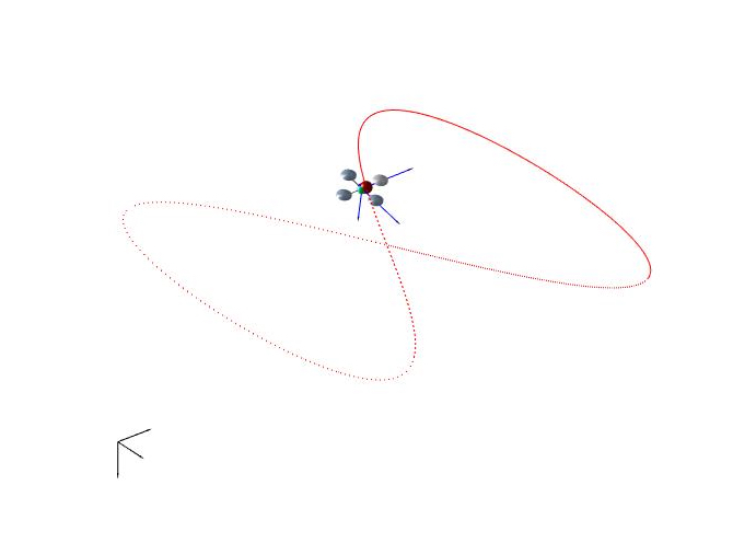
In this example, we investigate a case where noisy measurements on position, attitude and angular velocity are available via sensors and we wish to estimate the translational velocity while improving the noisy measurements. The measurements noise covariance is chosen as โ„›=1.0โ„›1.0\mathcal{R}=1.0 with process noise of ๐’ฌ=0.01๐’ฌ0.01\mathcal{Q}=0.01. Also the initial estimation values are chosen as xยฏโ€‹(0)=vยฏโ€‹(0)=[4,4,โˆ’3]Tยฏ๐‘ฅ0ยฏ๐‘ฃ0superscript443๐‘‡\bar{x}(0)=\bar{v}(0)=[4,4,-3]^{T} to have large initial estimation errors. Desired trajectory is chosen to be a Lissajous curve as

xdโ€‹(t)=[sinโก(t)+ฯ€2,sinโก(2โ€‹t),โˆ’0.5]T,b1โ€‹d=[1,โ€„0,โ€„0]T.formulae-sequencesubscript๐‘ฅ๐‘‘๐‘กsuperscript๐‘ก๐œ‹22๐‘ก0.5๐‘‡subscript๐‘1๐‘‘superscript1โ€„0โ€„0๐‘‡\displaystyle x_{d}(t)=[\sin(t)+\frac{\pi}{2},\;\sin(2t),\;-0.5]^{T},\;b_{1d}=[1,\;0,\;0]^{T}.

and geometric nonlinear controller is employed along with proposed EKF to track the above desired trajectory. The observation matrix, Hโˆˆโ„9ร—18๐ปsuperscriptโ„918H\in\mathbb{R}^{9\times 18} utilized in this example is

H=[I30000000I3000000I300].๐ปmatrixsubscript๐ผ30000000subscript๐ผ3000000subscript๐ผ300\displaystyle H=\begin{bmatrix}I_{3}&0&0&0&0&0\\ 0&0&I_{3}&0&0&0\\ 0&0&0&I_{3}&0&0\end{bmatrix}.

Refer to caption
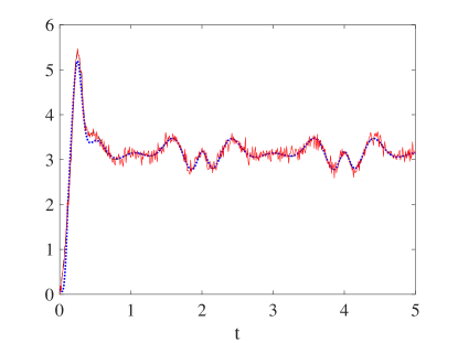
(a) Quadrotor position, x๐‘ฅx, x^^๐‘ฅ\hat{x}
Refer to caption
(b) ฮฉ1subscriptฮฉ1\Omega_{1}, ฮฉ^1subscript^ฮฉ1\hat{\Omega}_{1}

Refer to caption
(c) Quadrotor velocity, v๐‘ฃv, v^^๐‘ฃ\hat{v}
Refer to caption
(d) ฮฉ2subscriptฮฉ2\Omega_{2}, ฮฉ^2subscript^ฮฉ2\hat{\Omega}_{2}

Refer to caption
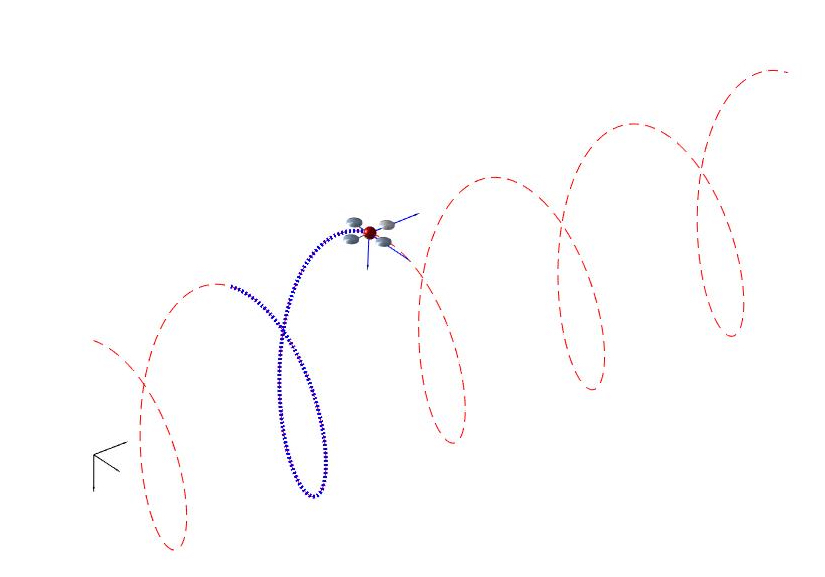
(e) 3D view, x๐‘ฅx, x^^๐‘ฅ\hat{x}
Refer to caption
(f) ฮฉ3subscriptฮฉ3\Omega_{3}, ฮฉ^3subscript^ฮฉ3\hat{\Omega}_{3}

Refer to caption
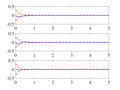
(g) Position error
Refer to caption
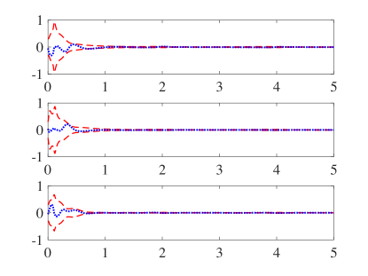
(h) Velocity error
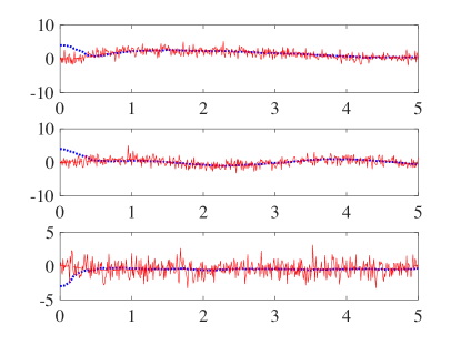
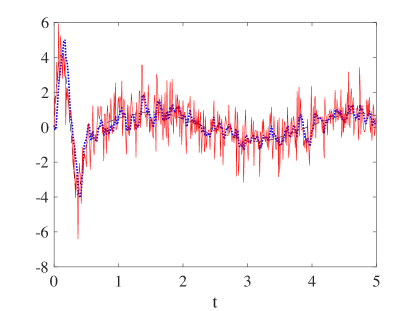
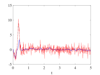
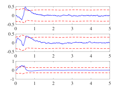
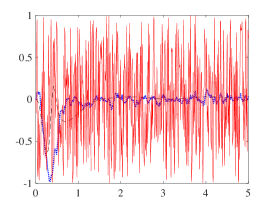
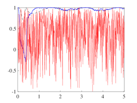
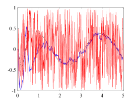
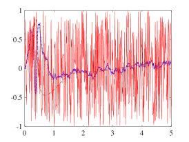
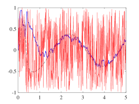
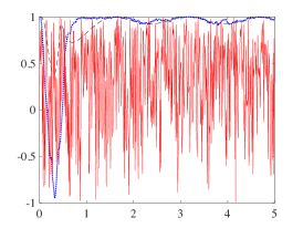
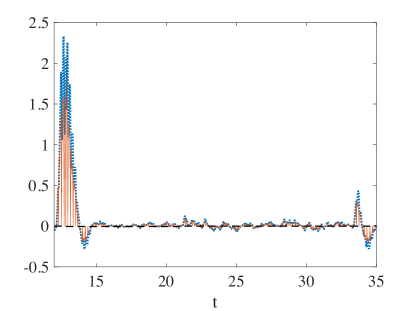
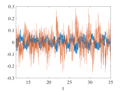
Figure 2: EKF performance in the first numerical example (dotted: EKF, dashed: desired, solid: noisy measurements). A short animation is also available at https://youtu.be/F4Vntws97RU

Figure 2 illustrates the performance of the proposed controller and EKF in this numerical simulation. Estimated position, xยฏยฏ๐‘ฅ\bar{x} and angular velocity, ฮฉฮฉ\Omega of the quadrotor is presented along with the noisy measurements at Figures 2(a), 2(b), 2(d), and 2(f) respectively. Desired translational velocity and the estimated velocity outputted from proposed EKF is plotted at Figure 2(c) which shows s satisfactory estimate during the maneuver. Figures 2(g) and 2(h) are the position and velocity estimation errors calculated from the following expressions.
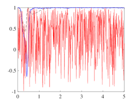
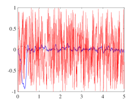
eยฏx=xยฏโˆ’xd,eยฏv=vยฏโˆ’vd.formulae-sequencesubscriptยฏ๐‘’๐‘ฅยฏ๐‘ฅsubscript๐‘ฅ๐‘‘subscriptยฏ๐‘’๐‘ฃยฏ๐‘ฃsubscript๐‘ฃ๐‘‘\displaystyle\bar{e}_{x}=\bar{x}-x_{d},\;\bar{e}_{v}=\bar{v}-v_{d}.

Refer to caption
(a) R11subscript๐‘…11R_{11}
Refer to caption
(b) R12subscript๐‘…12R_{12}
Refer to caption
(c) R13subscript๐‘…13R_{13}

Refer to caption
(d) R21subscript๐‘…21R_{21}
Refer to caption
(e) R22subscript๐‘…22R_{22}
Refer to caption
(f) R23subscript๐‘…23R_{23}

Refer to caption
(g) R31subscript๐‘…31R_{31}
Refer to caption
(h) R32subscript๐‘…32R_{32}
Refer to caption
(i) R33subscript๐‘…33R_{33}
Figure 3: EKF performance in the first numerical example for quadrotor rotation matrix (dotted: EKF, dashed: desired, solid: noisy measurements). A short animation is also available at https://youtu.be/Dfi3IljfS-U

We have also illustrated the attitude of the quadrotor as a rotation matrix in Figure 3. Noisy measurement data from sensor are presented along with the estimated attitude obtained from the proposed EKF and the desired attitude, Rdsubscript๐‘…๐‘‘R_{d}.

V-B Example 2- GPS denied environment

Assume that we receive measurements for attitude and angular velocity from an (Inertial Measurement Unit), IMU installed onboard and there is no sensor or measurements available for position and translational velocity for the quadrotor. In other words, we present a scenario where GPS systems fails to work. In this case our measurement vector, zโˆˆโ„3ร—๐–ฒ๐–ฎโ€‹(๐Ÿฅ)๐‘งsuperscriptโ„3๐–ฒ๐–ฎ3z\in\mathbb{R}^{3}\times\mathsf{SO(3)} consists of the angular velocity and the gravitational acceleration. The measurements noise covariance is chosen as โ„›=0.1โ„›0.1\mathcal{R}=0.1 with process noise of ๐’ฌ=0.001๐’ฌ0.001\mathcal{Q}=0.001 and initial estimates of the state variables are given by xยฏโ€‹(0)=[0.2,โˆ’0.5,โˆ’0.5]Tยฏ๐‘ฅ0superscript0.20.50.5๐‘‡\bar{x}(0)=[0.2,-0.5,-0.5]^{T} and vยฏโ€‹(0)=[0.1,โˆ’0.1,โˆ’0.1]Tยฏ๐‘ฃ0superscript0.10.10.1๐‘‡\bar{{v}}(0)=[0.1,-0.1,-0.1]^{T}. Desired trajectory is chosen to be an Elliptic Helix as

xdโ€‹(t)=[0.4โ€‹t,aโ€‹sinโก(wโ€‹t),โˆ’bโ€‹cosโก(wโ€‹t)]T,subscript๐‘ฅ๐‘‘๐‘กsuperscript0.4๐‘ก๐‘Ž๐‘ค๐‘ก๐‘๐‘ค๐‘ก๐‘‡\displaystyle x_{d}(t)=[0.4t,\;a\sin(wt),\;-b\cos(wt)]^{T},
b1โ€‹d=[cosโก(wโ€‹t),sinโก(wโ€‹t),โ€„0]T,subscript๐‘1๐‘‘superscript๐‘ค๐‘ก๐‘ค๐‘กโ€„0๐‘‡\displaystyle b_{1d}=[\cos(wt),\;\sin(wt),\;0]^{T},

where constants a=0.4๐‘Ž0.4a=0.4, b=0.6๐‘0.6b=0.6, w=ฯ€๐‘ค๐œ‹w=\pi and chosen particularly with several rotations of the quadrotor to illustrate the effectiveness of the proposed controller and extended kalman filter on ๐–ฒ๐–คโ€‹(๐Ÿฅ)๐–ฒ๐–ค3\mathsf{SE(3)} which does not concerns with singularities and ambiguities as seen in derivations with Euler angles or quaternions.
Refer to caption
(a) Quadrotor position, x๐‘ฅx, x^^๐‘ฅ\hat{x}
Refer to caption
(b) ฮฉ1subscriptฮฉ1\Omega_{1}, ฮฉ^1subscript^ฮฉ1\hat{\Omega}_{1}

Refer to caption
(c) Quadrotor velocity, v๐‘ฃv, v^^๐‘ฃ\hat{v}
Refer to caption
(d) ฮฉ2subscriptฮฉ2\Omega_{2}, ฮฉ^2subscript^ฮฉ2\hat{\Omega}_{2}

Refer to caption
(e) 3D view, x๐‘ฅx, x^^๐‘ฅ\hat{x}
Refer to caption
(f) ฮฉ3subscriptฮฉ3\Omega_{3}, ฮฉ^3subscript^ฮฉ3\hat{\Omega}_{3}

Refer to caption
(g) Position error
Refer to caption
(h) Velocity error
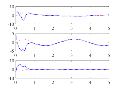
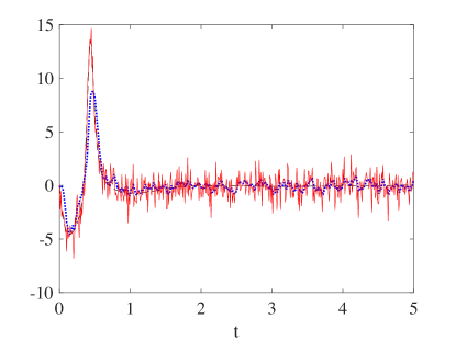
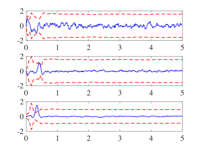
Figure 4: EKF performance in the second numerical example (dotted: EKF, dashed: desired, solid: noisy measurements). A short animation is also available at https://youtu.be/F4Vntws97RU

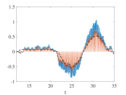
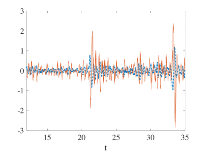
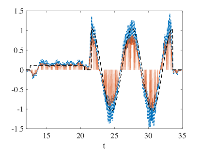
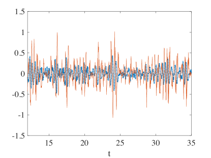
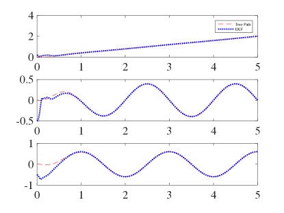
Figures 4(a) and 4(c) illustrate the position and velocity of the quadrotor estimated with EKF and plotted verse the true path respectively. As it is clear from this figure, although we did not have measurements on position and translational velocity, EKF was able to estimate this values significantly. Position and velocity estimation errors are also presented in Figures 4(g) and 4(h) respectively.
Figures 4(b), 4(d), and 4(f) illustrate the angular velocity of the quadrotor during this maneuver. Noisy measurement data and the estimated value from EKF are presented along with the true path to show the performance and effectiveness of the EKF to reduce the error and improve noisy measurements. Position and velocity estimation errors for this example are presented in Figures 4(g) and 4(h).

VI Experimental Results

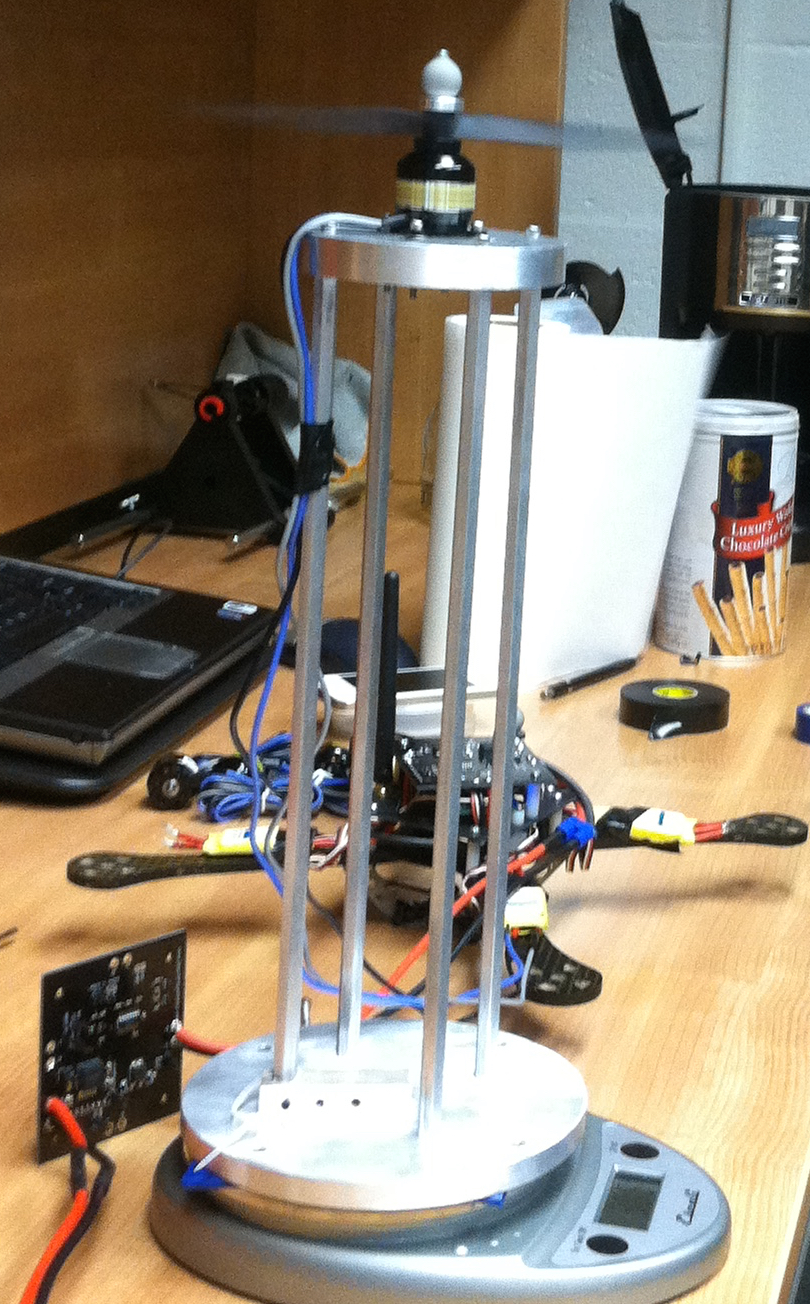
The quadrotor UAV developed at the flight dynamics and control laboratory at the George Washington University is shown at Figureย 5(a). We developed an accurate CAD model as shown in Figureย 1 to identify several parameters of the quadrotor, such as moment of inertia and center of mass. Furthermore, a precise rotor calibration is performed for each rotor, with a custom-made thrust stand as shown in Figureย 5(b) to determine the relation between the command in the motor speed controller and the actual thrust. For various values of motor speed commands, the corresponding thrust is measured, and those data are fitted with a second order polynomial.
Refer to caption OMAP 600MHz Processor Attitude sensor 3DM-GX3 via UART BLDC Motor via I2C Safety Switch XBee RF WIFI to Ground Station LiPo Battery 11.1V, 2200mAh
(a) Hardware configuration
Refer to caption
(b) Motor calibration setup
Figure 5: Hardware development for a quadrotor UAV

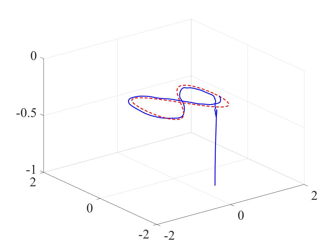
Angular velocity and attitude are measured from inertial measurement unit (IMU). Position of the UAV is measured from motion capture system (Vicon). Ground computing system receives the Vicon data and send it to the UAV via XBee. The Gumstix is adopted as micro computing unit on the UAV. A multi-threaded C/C++ software developed for autonomous control of the quadrotor. It has two main threads, namely Vicon thread, control and estimation thread. The Vicon thread receives the Vicon measurement. In second thread, it receives the IMU measurement, estimates the velocity with EKF and handles the control outputs. Figures 6 presents the experimental results for a maneuver where quadrotor autonomously tracks the following desired trajectory which is defined as a Lissajous curve
xdโ€‹(t)=[sinโก(t)+ฯ€2,sinโก2โ€‹(t),โˆ’0.3].subscript๐‘ฅ๐‘‘๐‘ก๐‘ก๐œ‹22๐‘ก0.3\displaystyle x_{d}(t)=[\sin(t)+\frac{\pi}{2},\;\sin 2(t),\;-0.3].

Refer to caption
(a) x๐‘ฅx, xdsubscript๐‘ฅ๐‘‘x_{d}
Refer to caption
(b) ฮจฮจ\Psi, eRsubscript๐‘’๐‘…e_{R}, eฮฉsubscript๐‘’ฮฉe_{\Omega}

Refer to caption
(c) dโ€‹x1dโ€‹t๐‘‘subscript๐‘ฅ1๐‘‘๐‘ก\frac{dx_{1}}{dt}, vd1subscript๐‘ฃsubscript๐‘‘1v_{d_{1}}, v^1subscript^๐‘ฃ1\hat{v}_{1}
Refer to caption
(d) ฮฉ1subscriptฮฉ1\Omega_{1}, ฮฉ^1subscript^ฮฉ1\hat{\Omega}_{1}

Refer to caption
(e) dโ€‹x2dโ€‹t๐‘‘subscript๐‘ฅ2๐‘‘๐‘ก\frac{dx_{2}}{dt}, vd1subscript๐‘ฃsubscript๐‘‘1v_{d_{1}}, v^2subscript^๐‘ฃ2\hat{v}_{2}
Refer to caption
(f) ฮฉ2subscriptฮฉ2\Omega_{2}, ฮฉ^2subscript^ฮฉ2\hat{\Omega}_{2}

Refer to caption
(g) dโ€‹x3dโ€‹t๐‘‘subscript๐‘ฅ3๐‘‘๐‘ก\frac{dx_{3}}{dt}, vd1subscript๐‘ฃsubscript๐‘‘1v_{d_{1}}, v^3subscript^๐‘ฃ3\hat{v}_{3}
Refer to caption
(h) ฮฉ3subscriptฮฉ3\Omega_{3}, ฮฉ^3subscript^ฮฉ3\hat{\Omega}_{3}
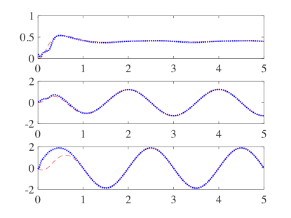
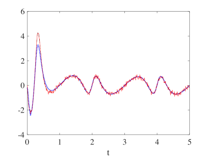
Figure 6: EKF performance in real-time experiment (dotted: EKF, dashed: desired, solid: noisy measurements).

Quadrotor parameters are same as presented in the numerical simulations section and controller gains are tuned to kx=4.0subscript๐‘˜๐‘ฅ4.0k_{x}=4.0, kv=2.0subscript๐‘˜๐‘ฃ2.0k_{v}=2.0, kR=0.62subscript๐‘˜๐‘…0.62k_{R}=0.62, kฮฉ=0.15subscript๐‘˜ฮฉ0.15k_{\Omega}=0.15, and kI=0.1subscript๐‘˜๐ผ0.1k_{I}=0.1 with c1=c2=0.1subscript๐‘1subscript๐‘20.1c_{1}=c_{2}=0.1. The observation matrix, Hโˆˆโ„9ร—18๐ปsuperscriptโ„918H\in\mathbb{R}^{9\times 18} utilized in this example same as one presented in the first numerical simulation and so for measurement state, ๐ณkโˆˆโ„9ร—1subscript๐ณ๐‘˜superscriptโ„91\mathbf{z}_{k}\in\mathbb{R}^{9\times 1}.

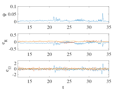
Figure 6(a) illustrates the position of the quadrotor following the desired trajectory obtained from the experiment. The quadrotor starts from the ground, increases its altitude to get to z3=โˆ’0.3โ€‹msubscript๐‘ง30.3mz_{3}=-0.3\ \mathrm{m}, and starts following the trajectory. Quadrotor attitude errors, ฮจฮจ\Psi, eRsubscript๐‘’๐‘…e_{R}, and angular velocity error, eฮฉsubscript๐‘’ฮฉe_{\Omega}, which are previously defined in Eq. (6), (7), and (8), respectively, are presented in Figure 6(b), which illustrate the performance of the geometric nonlinear controller during the autonomous trajectory tracking in this test. Figures 6(c), 6(e), and 6(g) illustrate the estimated velocity obtained form EKF namely, v^^๐‘ฃ\hat{v} and plotted verse the desired velocity, vdsubscript๐‘ฃ๐‘‘v_{d}. We have also presented the integrated velocity, dโ€‹xdโ€‹t๐‘‘๐‘ฅ๐‘‘๐‘ก\frac{dx}{dt} in this figure by taking direct derivative from the position measurements to magnify the performance of the filter. Figures 6(d), 6(f), and 6(h) are also present the angular velocity measurements from IMU, and the estimated angular velocity from the EKF, ฮฉ^^ฮฉ\hat{\Omega}. As it is clear from the figures, EKF is able to improve the measurement noises significantly and provide more smoother data for real-time experimentation. The effect of noise from velocity measurements is substantially reduced with the extended Kalman filter, while avoiding any lagging issues common with low-pass filtering.

VII CONCLUSIONS

An extensive Extended Kalman Filter on ๐–ฒ๐–คโ€‹(๐Ÿฅ)๐–ฒ๐–ค3\mathsf{SE(3)} for full nonlinear dynamic model of quadrotor UAV employing geometric nonlinear controller presented in this paper. Linearization performed considering all the coupling effects between translational and rotational dynamics to provide an precise estimation characteristics in different scenarios of sensor failure or receiving highly noised measurements. These results validated by numerical simulations followed by experimental results for velocity estimation during an autonomous trajectory tracking.

Acknowledgment

The authors would like to acknowledge Evan Kaufman for his helpful comments that served to improve the clarity of the discussion and writing of this paper.

References

  • [1] D.ย Mellinger, M.ย Shomin, N.ย Michael, and V.ย Kumar, โ€œCooperative grasping and transport using multiple quadrotors,โ€ in Distributed Autonomous Robotic Systems.ย ย ย Springer Berlin Heidelberg, 2013, vol.ย 83, pp. 545โ€“558.
  • [2] S.ย Kim, S.ย Choi, and H.ย J. Kim, โ€œAerial manipulation using a quadrotor with a two dof robotic arm,โ€ in Intelligent Robots and Systems, November 2013, pp. 4990โ€“4995.
  • [3] F.ย A. Goodarzi, D.ย Lee, and T.ย Lee, โ€œGeometric stabilization of quadrotor UAV with a payload connected by flexible cable,โ€ in Proceedings of American Control Conference, Portland OR, 2014, pp. 4925โ€“4930.
  • [4] G.ย N. Kostasย Alexis, Christosย Papachristos and A.ย Tzes, โ€œModel predictive quadrotor indoor position control,โ€ IEEE, 19th Mediterranean Conference on Control and Automation, pp. 1247โ€“1252, June 2011.
  • [5] I.ย Gumusboga and E.ย Kiyak, โ€œAn integrated navigation system design for quadrotors,โ€ Sensor Data Fusion: Trends, Solutions, Applications (SDF), pp. 1โ€“5, October 2015.
  • [6] K.-H. Oh and H.-S. Ahn, โ€œExtended kalman filter with multi-frequency reference data for quadrotor navigation,โ€ IEEE, 15th International Conference on Control, Automation and Systems (ICCAS 2015), pp. 201โ€“206, October 2015.
  • [7] F.ย C. Majidย Moghadam, โ€œActuator and sensor fault detection and diagnosis of quadrotor based on two-stage kalman filter,โ€ IEEE, 5th Australian Control Conference (AUCC), pp. 182โ€“187, November 2015.
  • [8] N.ย G. Frankย Hoffmann and T.ย Bertram, โ€œAttitude estimation and control of a quadrocopter,โ€ The 2010 IEEE/RSJ International Conference on Intelligent Robots and Systems, pp. 1072โ€“1077, October 2010.
  • [9] S.ย Wang and Y.ย Yang, โ€œQuadrotor aircraft attitude estimation and control based on kalman filter,โ€ IEEE, Proceedings of 31st Chinese Control Conference, pp. 5634โ€“5639, July 2012.
  • [10] Y.ย Z. Yilinย Hong, Xueqiuย Lin and Y.ย Zhao, โ€œReal-time pose estimation and motion control for a quadrotor uav,โ€ Proceeding of the 11th World Congress on Intelligent Control and Automation, pp. 2370โ€“2375, 2014.
  • [11] S.ย Bhat and D.ย Bernstein, โ€œA topological obstruction to continuous global stabilization of rotational motion and the unwinding phenomenon,โ€ Systems and Control Letters, vol.ย 39, pp. 66โ€“73, 2000.
  • [12] K.ย K. A.ย B. Samirย Zeghlache, Djamelย Saigaa, โ€œState vector estimation using extended filter kalman for the sliding mode controlled quadrotor helicopter in vertical flight,โ€ 8th International Conference on Electrical and Electronics Engineering (ELECO), pp. 492โ€“496, November 2013.
  • [13] F.ย A. Goodarzi and T.ย Lee, โ€œDynamics and control of quadrotor UAVs transporting a rigid body connected via flexible cables,โ€ in Proceedings of American Control Conference, Chicago IL, 2015, pp. 4677โ€“4682.
  • [14] F.ย A. Goodarzi, D.ย Lee, and T.ย Lee, โ€œGeometric control of a quadrotor UAV transporting a payload connected via flexible cable,โ€ International Journal of Control, Automation and Systems, vol.ย 13, no.ย 6, December 2015.
  • [15] F.ย A. Goodarzi, โ€œGeometric nonlinear controls for multiple cooperative quadrotor UAVs transporting a rigid body,โ€ Ph.D. dissertation, The George Washington University, August 2015.
  • [16] F.ย Goodarzi, D.ย Lee, and T.ย Lee, โ€œGeometric nonlinear PID control of a quadrotor UAV on ๐–ฒ๐–คโ€‹(๐Ÿฅ)๐–ฒ๐–ค3\mathsf{SE(3)},โ€ in in Proceedings of the European Control Conference, 2013, pp. 3845โ€“3850.
  • [17] F.ย A. Goodarzi, D.ย Lee, and T.ย Lee, โ€œGeometric adaptive tracking control of a quadrotor unmanned aerial vehicle on ๐–ฒ๐–คโ€‹(๐Ÿฅ)๐–ฒ๐–ค3\mathsf{SE(3)} for agile maneuvers,โ€ Journal of Dynamic Systems, Measurement, and Control, vol. 137, no.ย 9, pp. 091โ€‰007โ€“12, September 2015.
  • [18] F.ย Bullo and A.ย Lewis, Geometric control of mechanical systems, ser. Texts in Applied Mathematics.ย ย ย Springer, 2005, vol.ย 49, modeling, analysis, and design for simple mechanical control systems.
  • [19] T.ย Lee, โ€œRobust adaptive tracking on ๐–ฒ๐–ฎโ€‹(๐Ÿฅ)๐–ฒ๐–ฎ3\mathsf{SO(3)} with an application to the attitude dynamics of a quadrotor UAV,โ€ IEEE Transactions on Control Systems Technology, vol.ย 21, no.ย 5, pp. 1924โ€“1930, 2013.
  • [20] K.ย Subbarao, โ€œNonlinear PID-like controllers for rigid-body attitude stabilization,โ€ Journal of the Astronautical Sciences, vol.ย 52, no. 1-2, pp. 61โ€“74, 2004.
  • [21] K.ย Subbarao and M.ย Akella, โ€œDifferentiator-free nonlinear proportional-integral controllers for rigid-body attitude stabilization,โ€ Journal of Guidance, Control, and Dynamics, vol.ย 27, no.ย 6, pp. 1092โ€“1096, 2004.
  • [22] L.ย Show, J.ย Juang, C.ย Lin, and Y.ย Jan, โ€œSpacecraft robust attitude tracking design: PID control approach,โ€ in Proceeding of the American Control Conference, 1360-1365, Ed., 2002.
  • [23] M.ย L. T.ย Lee and N.ย McClamroch, โ€œNonlinear robust tracking control of a quadrotor UAV on ๐–ฒ๐–คโ€‹(๐Ÿฅ)๐–ฒ๐–ค3\mathsf{SE(3)},โ€ Asian Journal of Control, vol.ย 15, no.ย 2, pp. 391โ€“408, Mar. 2013.
  • [24] J.ย C. Butcher, The numerical analysis of ordinary differential equations: Runge-Kutta and general linear methods.ย ย ย New York, NY, USA: Wiley-Interscience, 1987.

-A Proof for Proposition 5

We use the definition and properties of time derivative and variation to linearize the closed loop system. The variation of time derivative of each state in the nonlinear equations can be presented as follow

ฮดโ€‹xห™=ฮดโ€‹v,๐›ฟห™๐‘ฅ๐›ฟ๐‘ฃ\displaystyle\delta\dot{x}=\delta v, (30)
ฮดโ€‹vห™=m21โ€‹ฮดโ€‹x+m22โ€‹ฮดโ€‹v+m23โ€‹ฮท+m24โ€‹ฮดโ€‹eiโ€‹1,๐›ฟห™๐‘ฃsubscript๐‘š21๐›ฟ๐‘ฅsubscript๐‘š22๐›ฟ๐‘ฃsubscript๐‘š23๐œ‚subscript๐‘š24๐›ฟsubscript๐‘’๐‘–1\displaystyle\delta{\dot{v}}=m_{21}\delta x+m_{22}\delta v+m_{23}\eta+m_{24}\delta e_{i1}, (31)
ฮทห™=ฮดโ€‹ฮฉโˆ’ฮฉ^โ€‹ฮท,ห™๐œ‚๐›ฟฮฉ^ฮฉ๐œ‚\displaystyle\dot{\eta}=\delta\Omega-\hat{\Omega}\eta, (32)
ฮดโ€‹ฮฉห™=๐›ฟห™ฮฉabsent\displaystyle\delta\dot{\Omega}= m41โ€‹ฮดโ€‹x+m42โ€‹ฮดโ€‹v+m43โ€‹ฮทsubscript๐‘š41๐›ฟ๐‘ฅsubscript๐‘š42๐›ฟ๐‘ฃsubscript๐‘š43๐œ‚\displaystyle m_{41}\delta x+m_{42}\delta v+m_{43}\eta
+m44โ€‹ฮดโ€‹ฮฉ+m45โ€‹ฮดโ€‹eiโ€‹1โˆ’kIโ€‹Jโˆ’1โ€‹ฮดโ€‹eiโ€‹2,subscript๐‘š44๐›ฟฮฉsubscript๐‘š45๐›ฟsubscript๐‘’๐‘–1subscript๐‘˜๐ผsuperscript๐ฝ1๐›ฟsubscript๐‘’๐‘–2\displaystyle+m_{44}\delta\Omega+m_{45}\delta e_{i1}-k_{I}J^{-1}\delta e_{i2}, (33)
ฮดโ€‹eห™iโ€‹1=c1โ€‹ฮดโ€‹ex+ฮดโ€‹ev=c1โ€‹ฮดโ€‹x+ฮดโ€‹v,๐›ฟsubscriptห™๐‘’๐‘–1subscript๐‘1๐›ฟsubscript๐‘’๐‘ฅ๐›ฟsubscript๐‘’๐‘ฃsubscript๐‘1๐›ฟ๐‘ฅ๐›ฟ๐‘ฃ\displaystyle\delta\dot{e}_{i1}=c_{1}\delta e_{x}+\delta e_{v}=c_{1}\delta{x}+\delta{v}, (34)
ฮดโ€‹eห™iโ€‹2=๐›ฟsubscriptห™๐‘’๐‘–2absent\displaystyle\delta\dot{e}_{i2}= c2โ€‹ฮดโ€‹eR+ฮดโ€‹eฮฉsubscript๐‘2๐›ฟsubscript๐‘’๐‘…๐›ฟsubscript๐‘’ฮฉ\displaystyle c_{2}\delta e_{R}+\delta e_{\Omega}
=m61โ€‹ฮดโ€‹x+m62โ€‹ฮดโ€‹v+m63โ€‹ฮดโ€‹ฮท+m64โ€‹ฮดโ€‹ฮฉ+m65โ€‹ฮดโ€‹eiโ€‹1.absentsubscript๐‘š61๐›ฟ๐‘ฅsubscript๐‘š62๐›ฟ๐‘ฃsubscript๐‘š63๐›ฟ๐œ‚subscript๐‘š64๐›ฟฮฉsubscript๐‘š65๐›ฟsubscript๐‘’๐‘–1\displaystyle=m_{61}\delta{x}+m_{62}\delta{v}+m_{63}\delta{\eta}+m_{64}\delta{\Omega}+m_{65}\delta{e_{i1}}. (35)

where all the sub-matrices miโ€‹jsubscript๐‘š๐‘–๐‘—m_{ij} in the above expressions are presented in the following sections. These equations can be written in a matrix form as

๐ฑห™=ALโ€‹๐ฑ,ห™๐ฑsubscript๐ด๐ฟ๐ฑ\displaystyle\dot{\mathbf{x}}=A_{L}\mathbf{x}, (36)

where the state vector ๐ฑโˆˆโ„18ร—1๐ฑsuperscriptโ„181\mathbf{x}\in\mathbb{R}^{18\times 1} is given by

๐ฑ=[ฮดโ€‹x,ฮดโ€‹v,ฮท,ฮดโ€‹ฮฉ,ฮดโ€‹eiโ€‹1,ฮดโ€‹eiโ€‹2]T,๐ฑsuperscriptmatrix๐›ฟ๐‘ฅ๐›ฟ๐‘ฃ๐œ‚๐›ฟฮฉ๐›ฟsubscript๐‘’๐‘–1๐›ฟsubscript๐‘’๐‘–2๐‘‡\displaystyle\mathbf{x}=\begin{bmatrix}\delta{x},\delta v,\eta,\delta\Omega,\delta{e}_{i1},\delta{e}_{i2}\\ \end{bmatrix}^{T},

and matrix Akโˆˆโ„18ร—18subscript๐ด๐‘˜superscriptโ„1818A_{k}\in\mathbb{R}^{18\times 18}

AL=[0I0000m21m22m230m2400โˆ’ฮฉ^I000m41m42m43m44m45โˆ’kIโ€‹Jโˆ’1c1I0000m61m62m63m64m650].subscript๐ด๐ฟmatrix0๐ผ0000subscript๐‘š21subscript๐‘š22subscript๐‘š230subscript๐‘š2400^ฮฉ๐ผ000subscript๐‘š41subscript๐‘š42subscript๐‘š43subscript๐‘š44subscript๐‘š45subscript๐‘˜๐ผsuperscript๐ฝ1subscript๐‘1๐ผ0000subscript๐‘š61subscript๐‘š62subscript๐‘š63subscript๐‘š64subscript๐‘š650\displaystyle A_{L}=\begin{bmatrix}0&I&0&0&0&0\\ m_{21}&m_{22}&m_{23}&0&m_{24}&0\\ 0&-\hat{\Omega}&I&0&0&0\\ m_{41}&m_{42}&m_{43}&m_{44}&m_{45}&-k_{I}J^{-1}\\ c_{1}&I&0&0&0&0\\ m_{61}&m_{62}&m_{63}&m_{64}&m_{65}&0\end{bmatrix}. (37)

-B Proof for Equation (31)

By taking time-derivative of both sides of Eq.ย (2), we would have

mโ€‹ฮดโ€‹vห™=โˆ’ฮดโ€‹fโ€‹Rโ€‹eeโˆ’fโ€‹ฮดโ€‹Rโ€‹e3=โˆ’ฮดโ€‹fโ€‹Rโ€‹eeโˆ’fโ€‹Rโ€‹ฮท^โ€‹e3,๐‘š๐›ฟห™๐‘ฃ๐›ฟ๐‘“๐‘…subscript๐‘’๐‘’๐‘“๐›ฟ๐‘…subscript๐‘’3๐›ฟ๐‘“๐‘…subscript๐‘’๐‘’๐‘“๐‘…^๐œ‚subscript๐‘’3\displaystyle m\delta{\dot{v}}=-\delta{f}Re_{e}-f\delta{R}e_{3}=-\delta{f}Re_{e}-fR\hat{\eta}e_{3}, (38)

using (15) and

ฮดโ€‹A=โˆ’kxโ€‹ฮดโ€‹exโˆ’kvโ€‹ฮดโ€‹ev,๐›ฟ๐ดsubscript๐‘˜๐‘ฅ๐›ฟsubscript๐‘’๐‘ฅsubscript๐‘˜๐‘ฃ๐›ฟsubscript๐‘’๐‘ฃ\displaystyle\delta{A}=-k_{x}\delta{e}_{x}-k_{v}\delta{e}_{v}, (39)

we obtain

ฮดโ€‹f=โˆ’(โˆ’kxโ€‹ฮดโ€‹xโˆ’kvโ€‹ฮดโ€‹v)โ‹…Rโ€‹3eโˆ’Aโ‹…Rโ€‹ฮท^โ€‹e3.๐›ฟ๐‘“โ‹…subscript๐‘˜๐‘ฅ๐›ฟ๐‘ฅsubscript๐‘˜๐‘ฃ๐›ฟ๐‘ฃ๐‘…subscript3๐‘’โ‹…๐ด๐‘…^๐œ‚subscript๐‘’3\displaystyle\delta f=-(-k_{x}\delta x-k_{v}\delta v)\cdot R3_{e}-A\cdot R\hat{\eta}e_{3}. (40)

Substituting the above equations into (38) and simplifying

ฮดโ€‹vห™=m21โ€‹ฮดโ€‹x+m22โ€‹ฮดโ€‹v+m23โ€‹ฮท+m24โ€‹ฮดโ€‹eiโ€‹1,๐›ฟห™๐‘ฃsubscript๐‘š21๐›ฟ๐‘ฅsubscript๐‘š22๐›ฟ๐‘ฃsubscript๐‘š23๐œ‚subscript๐‘š24๐›ฟsubscript๐‘’๐‘–1\displaystyle\delta{\dot{v}}=m_{21}\delta x+m_{22}\delta v+m_{23}\eta+m_{24}\delta e_{i1}, (41)

where m21,m22,m23,m24โˆˆโ„3ร—3subscript๐‘š21subscript๐‘š22subscript๐‘š23subscript๐‘š24superscriptโ„33m_{21},m_{22},m_{23},m_{24}\in\mathbb{R}^{3\times 3} are defined as

m21=โˆ’kxmโ€‹(Rโ€‹e3)โ€‹(Rโ€‹e3)T,m22=kvkxโ€‹m21,m24=kIkxโ€‹m21,formulae-sequencesubscript๐‘š21subscript๐‘˜๐‘ฅ๐‘š๐‘…subscript๐‘’3superscript๐‘…subscript๐‘’3๐‘‡formulae-sequencesubscript๐‘š22subscript๐‘˜๐‘ฃsubscript๐‘˜๐‘ฅsubscript๐‘š21subscript๐‘š24subscript๐‘˜๐ผsubscript๐‘˜๐‘ฅsubscript๐‘š21\displaystyle m_{21}=-\frac{k_{x}}{m}(Re_{3})(Re_{3})^{T},\;m_{22}=\frac{k_{v}}{k_{x}}m_{21},\;m_{24}=\frac{k_{I}}{k_{x}}m_{21}, (42)
m23=โˆ’1mโ€‹(Rโ€‹e3โ€‹ATโ€‹Rโ€‹e^3+(Aโ‹…Rโ€‹e3)โ€‹Rโ€‹e^3),subscript๐‘š231๐‘š๐‘…subscript๐‘’3superscript๐ด๐‘‡๐‘…subscript^๐‘’3โ‹…๐ด๐‘…subscript๐‘’3๐‘…subscript^๐‘’3\displaystyle m_{23}=-\frac{1}{m}(Re_{3}A^{T}R\hat{e}_{3}+(A\cdot Re_{3})R\hat{e}_{3}), (43)

-C Proof for Equation (32)

Taking derivative of Eq.ย (3), and using Eq.ย (22), we obtain

Rโ€‹ฮฉ^โ€‹ฮท^+Rโ€‹ฮทห™^=Rโ€‹ฮท^โ€‹ฮฉ^+Rโ€‹ฮดโ€‹ฮฉ^.๐‘…^ฮฉ^๐œ‚๐‘…^ห™๐œ‚๐‘…^๐œ‚^ฮฉ๐‘…๐›ฟ^ฮฉ\displaystyle R\hat{\Omega}\hat{\eta}+R\hat{\dot{\eta}}=R\hat{\eta}\hat{\Omega}+R\delta\hat{\Omega}. (44)

Multiplying both side of the above expression by Rโˆ’1superscript๐‘…1R^{-1}, using x^โ€‹y^โˆ’y^โ€‹x^=(xโ€‹y)โˆง^๐‘ฅ^๐‘ฆ^๐‘ฆ^๐‘ฅsuperscript๐‘ฅ๐‘ฆ\hat{x}\hat{y}-\hat{y}\hat{x}=(xy)^{\wedge} and simplifying, Eq. (32) is observed.

-D Proof for Equation (33)

We first find the variation of (7) and (8), considering (16) and simplify the equations utilizing ATโ€‹x^+x^โ€‹A=trโ€‹[A]โ€‹Iโˆ’Asuperscript๐ด๐‘‡^๐‘ฅ^๐‘ฅ๐ดtrdelimited-[]๐ด๐ผ๐ดA^{T}\hat{x}+\hat{x}A=\mathrm{tr}[A]I-A, to obtain

ฮดโ€‹eฮฉ=ฮดโ€‹ฮฉโˆ’(RTโ€‹Rdโ€‹ฮฉd)โˆงโ€‹ฮท+RTโ€‹Rdโ€‹ฮฉ^dโ€‹ฮทdโˆ’RTโ€‹Rdโ€‹ฮดโ€‹ฮฉd,๐›ฟsubscript๐‘’ฮฉ๐›ฟฮฉsuperscriptsuperscript๐‘…๐‘‡subscript๐‘…๐‘‘subscriptฮฉ๐‘‘๐œ‚superscript๐‘…๐‘‡subscript๐‘…๐‘‘subscript^ฮฉ๐‘‘subscript๐œ‚๐‘‘superscript๐‘…๐‘‡subscript๐‘…๐‘‘๐›ฟsubscriptฮฉ๐‘‘\displaystyle\delta e_{\Omega}=\delta\Omega-(R^{T}R_{d}\Omega_{d})^{\wedge}\eta+R^{T}R_{d}\hat{\Omega}_{d}\eta_{d}-R^{T}R_{d}\delta\Omega_{d}, (45)
ฮดโ€‹eR=12โ€‹(trโ€‹[RTโ€‹Rd]โ€‹Iโˆ’RTโ€‹Rd)โ€‹ฮทโˆ’12โ€‹(trโ€‹[RdTโ€‹R]โ€‹Iโˆ’RdTโ€‹R)โ€‹ฮทd.๐›ฟsubscript๐‘’๐‘…12trdelimited-[]superscript๐‘…๐‘‡subscript๐‘…๐‘‘๐ผsuperscript๐‘…๐‘‡subscript๐‘…๐‘‘๐œ‚12trdelimited-[]superscriptsubscript๐‘…๐‘‘๐‘‡๐‘…๐ผsuperscriptsubscript๐‘…๐‘‘๐‘‡๐‘…subscript๐œ‚๐‘‘\displaystyle\delta e_{R}=\frac{1}{2}(\mathrm{tr}[R^{T}R_{d}]I-R^{T}R_{d})\eta-\frac{1}{2}(\mathrm{tr}[R_{d}^{T}R]I-R_{d}^{T}R)\eta_{d}. (46)

Then, we need to find the variation for Rdsubscript๐‘…๐‘‘R_{d}, ฮฉdsubscriptฮฉ๐‘‘\Omega_{d} and their time-derivatives which are summarized below in each section. We utilize these derivations to find an explicit expression for the variation of Eq.ย (4) represented with the linearized state variables.

-D1 Variation of Rdsubscript๐‘…๐‘‘R_{d}

The desired attitude Rdsubscript๐‘…๐‘‘R_{d} is defined as follows

Rd=[b1โ€‹c,b2โ€‹c,b3โ€‹c]=[b2โ€‹cร—b3โ€‹c,b3โ€‹cร—b1โ€‹dโ€–b3โ€‹cร—b1โ€‹dโ€–,b3โ€‹c],subscript๐‘…๐‘‘subscript๐‘1๐‘subscript๐‘2๐‘subscript๐‘3๐‘subscript๐‘2๐‘subscript๐‘3๐‘subscript๐‘3๐‘subscript๐‘1๐‘‘normsubscript๐‘3๐‘subscript๐‘1๐‘‘subscript๐‘3๐‘\displaystyle R_{d}=[b_{1c},\,b_{2c},\,b_{3c}]=[b_{2c}\times b_{3c},\,\frac{b_{3c}\times b_{1d}}{\|b_{3c}\times b_{1d}\|},\,b_{3c}],

where

ฮดโ€‹b3โ€‹c=โˆ’ฮดโ€‹Aโ€–Aโ€–+Aโ€‹(Aโ‹…ฮดโ€‹A)โ€–Aโ€–3=b3โ€‹cร—(b3โ€‹cร—ฮดโ€‹Aโ€–Aโ€–).๐›ฟsubscript๐‘3๐‘๐›ฟ๐ดnorm๐ด๐ดโ‹…๐ด๐›ฟ๐ดsuperscriptnorm๐ด3subscript๐‘3๐‘subscript๐‘3๐‘๐›ฟ๐ดnorm๐ด\displaystyle\delta b_{3c}=-\frac{\delta{A}}{\|A\|}+\frac{A(A\cdot\delta{A})}{\|A\|^{3}}=b_{3c}\times(b_{3c}\times\frac{\delta A}{\|A\|}).

Using Eq. (39) and simplifying

ฮดโ€‹b3โ€‹c=z3ร—b3โ€‹c,z3=โˆ’b3โ€‹cร—ฮดโ€‹Aโ€–Aโ€–,formulae-sequence๐›ฟsubscript๐‘3๐‘subscript๐‘ง3subscript๐‘3๐‘subscript๐‘ง3subscript๐‘3๐‘๐›ฟ๐ดnorm๐ด\displaystyle\delta b_{3c}=z_{3}\times b_{3c},\;z_{3}=-b_{3c}\times\frac{\delta A}{\|A\|},

where z3โˆˆโ„3ร—1subscript๐‘ง3superscriptโ„31z_{3}\in\mathbb{R}^{3\times 1}. Similarly, the variation of b2โ€‹csubscript๐‘2๐‘b_{2c} and b1โ€‹csubscript๐‘1๐‘b_{1c} are given by

ฮดโ€‹b2โ€‹c=z2ร—b2โ€‹c,ฮดโ€‹b1โ€‹c=z1ร—b1โ€‹c,formulae-sequence๐›ฟsubscript๐‘2๐‘subscript๐‘ง2subscript๐‘2๐‘๐›ฟsubscript๐‘1๐‘subscript๐‘ง1subscript๐‘1๐‘\displaystyle\delta b_{2c}=z_{2}\times b_{2c},\;\delta b_{1c}=z_{1}\times b_{1c}, (47)

where vectors z1,z2โˆˆโ„3ร—1subscript๐‘ง1subscript๐‘ง2superscriptโ„31z_{1},z_{2}\in\mathbb{R}^{3\times 1} are defined as

z1=(b3โ€‹cโ‹…z2)โ€‹b3โ€‹c+(b2โ€‹cโ‹…z3)โ€‹b2โ€‹c,subscript๐‘ง1โ‹…subscript๐‘3๐‘subscript๐‘ง2subscript๐‘3๐‘โ‹…subscript๐‘2๐‘subscript๐‘ง3subscript๐‘2๐‘\displaystyle z_{1}=(b_{3c}\cdot z_{2})b_{3c}+(b_{2c}\cdot z_{3})b_{2c}, (48)
z2=b2โ€‹cร—((z3ร—b3โ€‹c)ร—b1โ€‹d)โ€–b3โ€‹cร—b1โ€‹dโ€–.subscript๐‘ง2subscript๐‘2๐‘subscript๐‘ง3subscript๐‘3๐‘subscript๐‘1๐‘‘normsubscript๐‘3๐‘subscript๐‘1๐‘‘\displaystyle z_{2}=\frac{b_{2c}\times((z_{3}\times b_{3c})\times b_{1d})}{\|b_{3c}\times b_{1d}\|}. (49)

From the above derivations, variation of Rdsubscript๐‘…๐‘‘R_{d} is given by

ฮดโ€‹Rd=[z1ร—b1โ€‹c,z2ร—b2โ€‹c,z3ร—b3โ€‹c].๐›ฟsubscript๐‘…๐‘‘subscript๐‘ง1subscript๐‘1๐‘subscript๐‘ง2subscript๐‘2๐‘subscript๐‘ง3subscript๐‘3๐‘\displaystyle\delta R_{d}=[z_{1}\times b_{1c},\,z_{2}\times b_{2c},\,z_{3}\times b_{3c}]. (50)

As Rdโˆˆ๐–ฒ๐–ฎโ€‹(๐Ÿฅ)subscript๐‘…๐‘‘๐–ฒ๐–ฎ3R_{d}\in\mathsf{SO(3)}, the variation of Rdsubscript๐‘…๐‘‘R_{d} can be written as ฮดโ€‹Rd=Rdโ€‹ฮท^d๐›ฟsubscript๐‘…๐‘‘subscript๐‘…๐‘‘subscript^๐œ‚๐‘‘\delta R_{d}=R_{d}\hat{\eta}_{d} for ฮทdโˆˆโ„3ร—1subscript๐œ‚๐‘‘superscriptโ„31\eta_{d}\in\mathbb{R}^{3\times 1}. Thus, using (50) and simplifying, ฮทdsubscript๐œ‚๐‘‘\eta_{d} is given by

ฮทd=(RdTโ€‹ฮดโ€‹Rd)โˆจ=a1โ€‹z3,subscript๐œ‚๐‘‘superscriptsuperscriptsubscript๐‘…๐‘‘๐‘‡๐›ฟsubscript๐‘…๐‘‘subscript๐‘Ž1subscript๐‘ง3\displaystyle\eta_{d}=(R_{d}^{T}\delta R_{d})^{\vee}=a_{1}z_{3},

where a1โˆˆโ„3ร—3subscript๐‘Ž1superscriptโ„33a_{1}\in\mathbb{R}^{3\times 3} is

a1=[b1โ€‹cT,b2โ€‹cT,(b1โ€‹dโ‹…b3โ€‹c)โ€–b3โ€‹cร—b1โ€‹dโ€–2โ€‹b1โ€‹dT]T.subscript๐‘Ž1superscriptsuperscriptsubscript๐‘1๐‘๐‘‡superscriptsubscript๐‘2๐‘๐‘‡โ‹…subscript๐‘1๐‘‘subscript๐‘3๐‘superscriptnormsubscript๐‘3๐‘subscript๐‘1๐‘‘2superscriptsubscript๐‘1๐‘‘๐‘‡๐‘‡\displaystyle a_{1}=[b_{1c}^{T},\;b_{2c}^{T},\;\frac{(b_{1d}\cdot b_{3c})}{\|b_{3c}\times b_{1d}\|^{2}}b_{1d}^{T}]^{T}. (51)

-D2 Variation of ฮฉdsubscriptฮฉ๐‘‘\Omega_{d}

We use the angular velocity equation ฮฉ^d=RdTโ€‹Rห™dsubscript^ฮฉ๐‘‘superscriptsubscript๐‘…๐‘‘๐‘‡subscriptห™๐‘…๐‘‘\hat{\Omega}_{d}=R_{d}^{T}\dot{R}_{d} and take variation from both sides. First we find an expression for the time derivative of Rdsubscript๐‘…๐‘‘R_{d} which is given as

Rห™d=[bห™1โ€‹c,bห™2โ€‹c,bห™3โ€‹c].subscriptห™๐‘…๐‘‘subscriptห™๐‘1๐‘subscriptห™๐‘2๐‘subscriptห™๐‘3๐‘\displaystyle\dot{R}_{d}=[\dot{b}_{1c},\,\dot{b}_{2c},\,\dot{b}_{3c}].

Similar to the pervious steps we can find an expression for

bห™3โ€‹c=ฮถ3ร—b3โ€‹c,bห™2โ€‹c=ฮถ2ร—b2โ€‹c,bห™1โ€‹c=ฮถ1ร—b1โ€‹c,formulae-sequencesubscriptห™๐‘3๐‘subscript๐œ3subscript๐‘3๐‘formulae-sequencesubscriptห™๐‘2๐‘subscript๐œ2subscript๐‘2๐‘subscriptห™๐‘1๐‘subscript๐œ1subscript๐‘1๐‘\displaystyle\dot{b}_{3c}=\zeta_{3}\times b_{3c},\;\dot{b}_{2c}=\zeta_{2}\times b_{2c},\;\dot{b}_{1c}=\zeta_{1}\times b_{1c}, (52)

where ฮถ1,ฮถ2,ฮถ3โˆˆโ„3ร—1subscript๐œ1subscript๐œ2subscript๐œ3superscriptโ„31\zeta_{1},\zeta_{2},\zeta_{3}\in\mathbb{R}^{3\times 1} are

ฮถ3=โˆ’b3โ€‹cร—Aห™โ€–Aโ€–,subscript๐œ3subscript๐‘3๐‘ห™๐ดnorm๐ด\displaystyle\zeta_{3}=-b_{3c}\times\frac{\dot{A}}{\|A\|}, (53)
ฮถ2=b2โ€‹cร—((ฮถ3ร—b3โ€‹c)ร—b1โ€‹d+b3โ€‹cร—bห™1โ€‹d)โ€–b3โ€‹cร—b1โ€‹dโ€–,subscript๐œ2subscript๐‘2๐‘subscript๐œ3subscript๐‘3๐‘subscript๐‘1๐‘‘subscript๐‘3๐‘subscriptห™๐‘1๐‘‘normsubscript๐‘3๐‘subscript๐‘1๐‘‘\displaystyle\zeta_{2}=\frac{b_{2c}\times((\zeta_{3}\times b_{3c})\times b_{1d}+b_{3c}\times\dot{b}_{1d})}{\|b_{3c}\times b_{1d}\|}, (54)
ฮถ1=(b3โ€‹cโ‹…ฮถ2)โ€‹b3โ€‹c+(b2โ€‹cโ‹…ฮถ3)โ€‹b2โ€‹c,subscript๐œ1โ‹…subscript๐‘3๐‘subscript๐œ2subscript๐‘3๐‘โ‹…subscript๐‘2๐‘subscript๐œ3subscript๐‘2๐‘\displaystyle\zeta_{1}=(b_{3c}\cdot\zeta_{2})b_{3c}+(b_{2c}\cdot\zeta_{3})b_{2c}, (55)

thus

Rห™d=[bห™1โ€‹c,bห™2โ€‹c,bห™3โ€‹c]=[ฮถ1ร—b1โ€‹c,ฮถ2ร—b2โ€‹c,ฮถ3ร—b3โ€‹c].subscriptห™๐‘…๐‘‘subscriptห™๐‘1๐‘subscriptห™๐‘2๐‘subscriptห™๐‘3๐‘subscript๐œ1subscript๐‘1๐‘subscript๐œ2subscript๐‘2๐‘subscript๐œ3subscript๐‘3๐‘\displaystyle\dot{R}_{d}=[\dot{b}_{1c},\,\dot{b}_{2c},\,\dot{b}_{3c}]=[\zeta_{1}\times b_{1c},\ \zeta_{2}\times b_{2c},\ \zeta_{3}\times b_{3c}].

Substituting the above expression into ฮฉ^d=RdTโ€‹Rห™dsubscript^ฮฉ๐‘‘superscriptsubscript๐‘…๐‘‘๐‘‡subscriptห™๐‘…๐‘‘\hat{\Omega}_{d}=R_{d}^{T}\dot{R}_{d} and simplifying, ฮฉdsubscriptฮฉ๐‘‘\Omega_{d} can be written as

ฮฉd=a1โ€‹ฮถ3+a2,subscriptฮฉ๐‘‘subscript๐‘Ž1subscript๐œ3subscript๐‘Ž2\displaystyle\Omega_{d}=a_{1}\zeta_{3}+a_{2},

where a2โˆˆโ„3ร—1subscript๐‘Ž2superscriptโ„31a_{2}\in\mathbb{R}^{3\times 1}

a2=[0,โ€„0,bห™1โ€‹dโ‹…b2โ€‹cโ€–b3โ€‹cร—b1โ€‹dโ€–]T.subscript๐‘Ž2superscript0โ€„0โ‹…subscriptห™๐‘1๐‘‘subscript๐‘2๐‘normsubscript๐‘3๐‘subscript๐‘1๐‘‘๐‘‡\displaystyle a_{2}=[0,\;0,\;\frac{\dot{b}_{1d}\cdot b_{2c}}{\|b_{3c}\times b_{1d}\|}]^{T}. (56)

Time-derivative of ฮทdsubscript๐œ‚๐‘‘\eta_{d} can be presented as

ฮทห™d=aห™1โ€‹z3+a1โ€‹zห™3.subscriptห™๐œ‚๐‘‘subscriptห™๐‘Ž1subscript๐‘ง3subscript๐‘Ž1subscriptห™๐‘ง3\displaystyle\dot{\eta}_{d}=\dot{a}_{1}z_{3}+a_{1}\dot{z}_{3}. (57)

After simplifying, we can present zห™3subscriptห™๐‘ง3\dot{z}_{3} as

zห™3=B1โ€‹ฮดโ€‹x+B2โ€‹ฮดโ€‹v+B3โ€‹ฮท+B4โ€‹ฮดโ€‹eiโ€‹1,subscriptห™๐‘ง3subscript๐ต1๐›ฟ๐‘ฅsubscript๐ต2๐›ฟ๐‘ฃsubscript๐ต3๐œ‚subscript๐ต4๐›ฟsubscript๐‘’๐‘–1\displaystyle\dot{z}_{3}=B_{1}\delta x+B_{2}\delta v+B_{3}\eta+B_{4}\delta e_{i1},

where sub-matrices B1,B2,B3,B4โˆˆโ„3ร—3subscript๐ต1subscript๐ต2subscript๐ต3subscript๐ต4superscriptโ„33B_{1},B_{2},B_{3},B_{4}\in\mathbb{R}^{3\times 3} are

B1=โˆ’kxโ€‹X1โˆ’kvโ€‹X2โ€‹m21โˆ’kIโ€‹B5โ€‹X2,subscript๐ต1subscript๐‘˜๐‘ฅsubscript๐‘‹1subscript๐‘˜๐‘ฃsubscript๐‘‹2subscript๐‘š21subscript๐‘˜๐ผsubscript๐ต5subscript๐‘‹2\displaystyle B_{1}=-k_{x}X_{1}-k_{v}X_{2}m_{21}-k_{I}B_{5}X_{2},
B2=โˆ’kvโ€‹X1โˆ’(kx+kI)โ€‹X2โˆ’kvโ€‹X2โ€‹m22,subscript๐ต2subscript๐‘˜๐‘ฃsubscript๐‘‹1subscript๐‘˜๐‘ฅsubscript๐‘˜๐ผsubscript๐‘‹2subscript๐‘˜๐‘ฃsubscript๐‘‹2subscript๐‘š22\displaystyle B_{2}=-k_{v}X_{1}-(k_{x}+k_{I})X_{2}-k_{v}X_{2}m_{22},
B3=โˆ’kvโ€‹X2โ€‹m23,B4=โˆ’kIโ€‹X1โˆ’kvโ€‹X2โ€‹m24,formulae-sequencesubscript๐ต3subscript๐‘˜๐‘ฃsubscript๐‘‹2subscript๐‘š23subscript๐ต4subscript๐‘˜๐ผsubscript๐‘‹1subscript๐‘˜๐‘ฃsubscript๐‘‹2subscript๐‘š24\displaystyle B_{3}=-k_{v}X_{2}m_{23},\;B_{4}=-k_{I}X_{1}-k_{v}X_{2}m_{24},

and X1,X2โˆˆโ„3ร—3subscript๐‘‹1subscript๐‘‹2superscriptโ„33X_{1},X_{2}\in\mathbb{R}^{3\times 3}

X1=โˆ’(bห™3โ€‹c)โˆงโ€–Aโ€–+(b3โ€‹c)โˆงโ€‹(Aโ‹…Aห™)โ€–Aโ€–3,X2=โˆ’(b3โ€‹c)โˆงโ€–Aโ€–.formulae-sequencesubscript๐‘‹1superscriptsubscriptห™๐‘3๐‘norm๐ดsuperscriptsubscript๐‘3๐‘โ‹…๐ดห™๐ดsuperscriptnorm๐ด3subscript๐‘‹2superscriptsubscript๐‘3๐‘norm๐ด\displaystyle X_{1}=-\frac{(\dot{b}_{3c})^{\wedge}}{\|A\|}+\frac{({b}_{3c})^{\wedge}(A\cdot\dot{A})}{\|A\|^{3}},\;X_{2}=-\frac{(b_{3c})^{\wedge}}{\|A\|}.

Substituting the time derivative of a1subscript๐‘Ž1a_{1} and the above expressions into Eq. (57)

ฮทห™d=B5โ€‹ฮดโ€‹x+B6โ€‹ฮดโ€‹v+B7โ€‹ฮท+kIโ€‹B9โ€‹ฮดโ€‹eiโ€‹1,subscriptห™๐œ‚๐‘‘subscript๐ต5๐›ฟ๐‘ฅsubscript๐ต6๐›ฟ๐‘ฃsubscript๐ต7๐œ‚subscript๐‘˜๐ผsubscript๐ต9๐›ฟsubscript๐‘’๐‘–1\displaystyle\dot{\eta}_{d}=B_{5}\delta x+B_{6}\delta v+B_{7}\eta+k_{I}B_{9}\delta e_{i1},

where B5,B6,B7,B8,B9โˆˆโ„3ร—3subscript๐ต5subscript๐ต6subscript๐ต7subscript๐ต8subscript๐ต9superscriptโ„33B_{5},B_{6},B_{7},B_{8},B_{9}\in\mathbb{R}^{3\times 3} are given by

B5=kxโ€‹aห™1โ€‹(b3โ€‹c)โˆงโ€–Aโ€–+a1โ€‹B1,B6=kvโ€‹aห™1โ€‹(b3โ€‹c)โˆงโ€–Aโ€–+a1โ€‹B2,formulae-sequencesubscript๐ต5subscript๐‘˜๐‘ฅsubscriptห™๐‘Ž1superscriptsubscript๐‘3๐‘norm๐ดsubscript๐‘Ž1subscript๐ต1subscript๐ต6subscript๐‘˜๐‘ฃsubscriptห™๐‘Ž1superscriptsubscript๐‘3๐‘norm๐ดsubscript๐‘Ž1subscript๐ต2\displaystyle B_{5}=\frac{k_{x}\dot{a}_{1}(b_{3c})^{\wedge}}{\|A\|}+a_{1}B_{1},\;B_{6}=\frac{k_{v}\dot{a}_{1}(b_{3c})^{\wedge}}{\|A\|}+a_{1}B_{2},
B7=a1โ€‹B3,B8=kIโ€‹aห™1โ€‹(b3โ€‹c)โˆงโ€–Aโ€–+a1โ€‹B4,B9=(ฮฉ^dโ€‹a1โ€‹(b3โ€‹cโˆง))โ€–Aโ€–.formulae-sequencesubscript๐ต7subscript๐‘Ž1subscript๐ต3formulae-sequencesubscript๐ต8subscript๐‘˜๐ผsubscriptห™๐‘Ž1superscriptsubscript๐‘3๐‘norm๐ดsubscript๐‘Ž1subscript๐ต4subscript๐ต9subscript^ฮฉ๐‘‘subscript๐‘Ž1superscriptsubscript๐‘3๐‘norm๐ด\displaystyle B_{7}=a_{1}B_{3},\;B_{8}=\frac{k_{I}\dot{a}_{1}(b_{3c})^{\wedge}}{\|A\|}+a_{1}B_{4},\;B_{9}=\frac{(\hat{\Omega}_{d}a_{1}(b_{3c}^{\wedge}))}{\|A\|}.

After simplifying, the variation of ฮฉdsubscriptฮฉ๐‘‘\Omega_{d} is given by

ฮดโ€‹ฮฉd=๐›ฟsubscriptฮฉ๐‘‘absent\displaystyle\delta\Omega_{d}= ฮทห™d+ฮฉ^dโ€‹ฮทdsubscriptห™๐œ‚๐‘‘subscript^ฮฉ๐‘‘subscript๐œ‚๐‘‘\displaystyle\dot{\eta}_{d}+\hat{\Omega}_{d}\eta_{d}
=\displaystyle= (B5+kxโ€‹B9)โ€‹ฮดโ€‹x+(B6+kvโ€‹B9)โ€‹ฮดโ€‹vsubscript๐ต5subscript๐‘˜๐‘ฅsubscript๐ต9๐›ฟ๐‘ฅsubscript๐ต6subscript๐‘˜๐‘ฃsubscript๐ต9๐›ฟ๐‘ฃ\displaystyle(B_{5}+k_{x}B_{9})\delta x+(B_{6}+k_{v}B_{9})\delta v
+B7โ€‹ฮท+(B8+kIโ€‹B9)โ€‹ฮดโ€‹eiโ€‹1.subscript๐ต7๐œ‚subscript๐ต8subscript๐‘˜๐ผsubscript๐ต9๐›ฟsubscript๐‘’๐‘–1\displaystyle+B_{7}\eta+(B_{8}+k_{I}B_{9})\delta e_{i1}. (58)

-D3 Time derivative of ฮดโ€‹ฮฉd๐›ฟsubscriptฮฉ๐‘‘\delta{\Omega}_{d}

Taking time derivative of Eq.ย (-D2), using ฮทห™=ฮดโ€‹ฮฉโˆ’ฮฉ^โ€‹ฮทห™๐œ‚๐›ฟฮฉ^ฮฉ๐œ‚\dot{\eta}=\delta\Omega-\hat{\Omega}\eta, and Eq. (41), we have

ฮดโ€‹ฮฉห™d=F1โ€‹ฮดโ€‹x+F2โ€‹ฮดโ€‹v+F3โ€‹ฮท+B7โ€‹ฮดโ€‹ฮฉ+F4โ€‹ฮดโ€‹eiโ€‹1,๐›ฟsubscriptห™ฮฉ๐‘‘subscript๐น1๐›ฟ๐‘ฅsubscript๐น2๐›ฟ๐‘ฃsubscript๐น3๐œ‚subscript๐ต7๐›ฟฮฉsubscript๐น4๐›ฟsubscript๐‘’๐‘–1\displaystyle\delta\dot{\Omega}_{d}=F_{1}\delta x+F_{2}\delta v+F_{3}\eta+B_{7}\delta\Omega+F_{4}\delta e_{i1},

where matrices F1,F2,F3,F4โˆˆโ„3ร—3subscript๐น1subscript๐น2subscript๐น3subscript๐น4superscriptโ„33F_{1},F_{2},F_{3},F_{4}\in\mathbb{R}^{3\times 3} are defined as

F1=Bห™5+kxโ€‹Bห™9+(B6+kvโ€‹B9)โ€‹A21+B5โ€‹(B8+kIโ€‹B9),subscript๐น1subscriptห™๐ต5subscript๐‘˜๐‘ฅsubscriptห™๐ต9subscript๐ต6subscript๐‘˜๐‘ฃsubscript๐ต9subscript๐ด21subscript๐ต5subscript๐ต8subscript๐‘˜๐ผsubscript๐ต9\displaystyle F_{1}=\dot{B}_{5}+k_{x}\dot{B}_{9}+(B_{6}+k_{v}B_{9})A_{21}+B_{5}(B_{8}+k_{I}B_{9}),
F2=subscript๐น2absent\displaystyle F_{2}= B5+kxโ€‹B9+Bห™6+kvโ€‹Bห™9subscript๐ต5subscript๐‘˜๐‘ฅsubscript๐ต9subscriptห™๐ต6subscript๐‘˜๐‘ฃsubscriptห™๐ต9\displaystyle B_{5}+k_{x}B_{9}+\dot{B}_{6}+k_{v}\dot{B}_{9}
+(B6+kvโ€‹B9)โ€‹A22+(B8+kIโ€‹B9),subscript๐ต6subscript๐‘˜๐‘ฃsubscript๐ต9subscript๐ด22subscript๐ต8subscript๐‘˜๐ผsubscript๐ต9\displaystyle+(B_{6}+k_{v}B_{9})A_{22}+(B_{8}+k_{I}B_{9}),
F3=(B6+kvโ€‹B9)โ€‹A23+Bห™7โˆ’B7โ€‹ฮฉ^,subscript๐น3subscript๐ต6subscript๐‘˜๐‘ฃsubscript๐ต9subscript๐ด23subscriptห™๐ต7subscript๐ต7^ฮฉ\displaystyle F_{3}=(B_{6}+k_{v}B_{9})A_{23}+\dot{B}_{7}-B_{7}\hat{\Omega},
F4=Bห™8+kIโ€‹Bห™9.subscript๐น4subscriptห™๐ต8subscript๐‘˜๐ผsubscriptห™๐ต9\displaystyle F_{4}=\dot{B}_{8}+k_{I}\dot{B}_{9}.

-D4 Variations of eiโ€‹1subscript๐‘’๐‘–1e_{i1} and eiโ€‹2subscript๐‘’๐‘–2e_{i2}

The variation of eiโ€‹1subscript๐‘’๐‘–1e_{i1} and eiโ€‹2subscript๐‘’๐‘–2e_{i2} can be expressed as

ฮดโ€‹eiโ€‹1=cโ€‹ฮดโ€‹ex+ฮดโ€‹ev=cโ€‹ฮดโ€‹x+ฮดโ€‹v,๐›ฟsubscript๐‘’๐‘–1๐‘๐›ฟsubscript๐‘’๐‘ฅ๐›ฟsubscript๐‘’๐‘ฃ๐‘๐›ฟ๐‘ฅ๐›ฟ๐‘ฃ\displaystyle\delta e_{i1}=c\delta e_{x}+\delta e_{v}=c\delta{x}+\delta{v},
ฮดโ€‹eiโ€‹2๐›ฟsubscript๐‘’๐‘–2\displaystyle\delta e_{i2} =cโ€‹ฮดโ€‹eR+ฮดโ€‹eฮฉabsent๐‘๐›ฟsubscript๐‘’๐‘…๐›ฟsubscript๐‘’ฮฉ\displaystyle=c\delta e_{R}+\delta e_{\Omega}
=m61โ€‹ฮดโ€‹x+m62โ€‹ฮดโ€‹v+m63โ€‹ฮดโ€‹ฮท+m64โ€‹ฮดโ€‹xโ€‹ฮฉ+m65โ€‹ฮดโ€‹eiโ€‹1,absentsubscript๐‘š61๐›ฟ๐‘ฅsubscript๐‘š62๐›ฟ๐‘ฃsubscript๐‘š63๐›ฟ๐œ‚subscript๐‘š64๐›ฟ๐‘ฅฮฉsubscript๐‘š65๐›ฟsubscript๐‘’๐‘–1\displaystyle=m_{61}\delta{x}+m_{62}\delta{v}+m_{63}\delta{\eta}+m_{64}\delta{x\Omega}+m_{65}\delta{e_{i1}},

where m61,m62,m63,m64,m65โˆˆโ„3ร—3subscript๐‘š61subscript๐‘š62subscript๐‘š63subscript๐‘š64subscript๐‘š65superscriptโ„33m_{61},m_{62},m_{63},m_{64},m_{65}\in\mathbb{R}^{3\times 3} are defined as

m61=โˆ’B5โ€‹G5โ€‹Y1+G2โ€‹Y1โˆ’G3โ€‹(B5+kxโ€‹B9),subscript๐‘š61subscript๐ต5subscript๐บ5subscript๐‘Œ1subscript๐บ2subscript๐‘Œ1subscript๐บ3subscript๐ต5subscript๐‘˜๐‘ฅsubscript๐ต9\displaystyle m_{61}=-B_{5}G_{5}Y_{1}+G_{2}Y_{1}-G_{3}(B_{5}+k_{x}B_{9}),
m62=โˆ’B5โ€‹G5โ€‹Y2+G2โ€‹Y1โˆ’G3โ€‹(B6+kvโ€‹B9),subscript๐‘š62subscript๐ต5subscript๐บ5subscript๐‘Œ2subscript๐บ2subscript๐‘Œ1subscript๐บ3subscript๐ต6subscript๐‘˜๐‘ฃsubscript๐ต9\displaystyle m_{62}=-B_{5}G_{5}Y_{2}+G_{2}Y_{1}-G_{3}(B_{6}+k_{v}B_{9}),
m63=B5โ€‹G4โˆ’G1โˆ’G3โ€‹B7,m64=I3ร—3,formulae-sequencesubscript๐‘š63subscript๐ต5subscript๐บ4subscript๐บ1subscript๐บ3subscript๐ต7subscript๐‘š64subscript๐ผ33\displaystyle m_{63}=B_{5}G_{4}-G_{1}-G_{3}B_{7},\;m_{64}=I_{3\times 3},
m65=โˆ’B5โ€‹G5โ€‹Y3+G2โ€‹Y3โˆ’G3โ€‹(B8+kIโ€‹B9),subscript๐‘š65subscript๐ต5subscript๐บ5subscript๐‘Œ3subscript๐บ2subscript๐‘Œ3subscript๐บ3subscript๐ต8subscript๐‘˜๐ผsubscript๐ต9\displaystyle m_{65}=-B_{5}G_{5}Y_{3}+G_{2}Y_{3}-G_{3}(B_{8}+k_{I}B_{9}),

and matrices G1,G2,G3,G4,G5โˆˆโ„3ร—3subscript๐บ1subscript๐บ2subscript๐บ3subscript๐บ4subscript๐บ5superscriptโ„33G_{1},G_{2},G_{3},G_{4},G_{5}\in\mathbb{R}^{3\times 3} are

G1=(RTโ€‹Rdโ€‹ฮฉd)โˆง,G2=RTโ€‹Rdโ€‹ฮฉd^,G3=RTโ€‹Rd,formulae-sequencesubscript๐บ1superscriptsuperscript๐‘…๐‘‡subscript๐‘…๐‘‘subscriptฮฉ๐‘‘formulae-sequencesubscript๐บ2superscript๐‘…๐‘‡subscript๐‘…๐‘‘^subscriptฮฉ๐‘‘subscript๐บ3superscript๐‘…๐‘‡subscript๐‘…๐‘‘\displaystyle G_{1}=(R^{T}R_{d}\Omega_{d})^{\wedge},G_{2}=R^{T}R_{d}\hat{\Omega_{d}},G_{3}=R^{T}R_{d},
G4=12โ€‹(trโ€‹[RTโ€‹Rd]โ€‹Iโˆ’RTโ€‹Rd),subscript๐บ412trdelimited-[]superscript๐‘…๐‘‡subscript๐‘…๐‘‘๐ผsuperscript๐‘…๐‘‡subscript๐‘…๐‘‘\displaystyle G_{4}=\frac{1}{2}(\mathrm{tr}[R^{T}R_{d}]I-R^{T}R_{d}),
G5=12โ€‹(trโ€‹[RdTโ€‹R]โ€‹Iโˆ’RdTโ€‹R).subscript๐บ512trdelimited-[]superscriptsubscript๐‘…๐‘‘๐‘‡๐‘…๐ผsuperscriptsubscript๐‘…๐‘‘๐‘‡๐‘…\displaystyle G_{5}=\frac{1}{2}(\mathrm{tr}[R_{d}^{T}R]I-R_{d}^{T}R).

-D5 Variation for Equation (4)

Substituting the above derivations for ฮดโ€‹ฮฉd๐›ฟsubscriptฮฉ๐‘‘\delta\Omega_{d}, ฮดโ€‹Rd๐›ฟsubscript๐‘…๐‘‘\delta R_{d} into Eq.ย (45), and (46) and simplifying, we can present the following expression for Eq.ย (4)

ฮดโ€‹ฮฉห™=๐›ฟห™ฮฉabsent\displaystyle\delta\dot{\Omega}= m41โ€‹ฮดโ€‹x+m42โ€‹ฮดโ€‹v+m43โ€‹ฮท+m44โ€‹ฮดโ€‹ฮฉsubscript๐‘š41๐›ฟ๐‘ฅsubscript๐‘š42๐›ฟ๐‘ฃsubscript๐‘š43๐œ‚subscript๐‘š44๐›ฟฮฉ\displaystyle m_{41}\delta x+m_{42}\delta v+m_{43}\eta+m_{44}\delta\Omega
+m45โ€‹ฮดโ€‹eiโ€‹1โˆ’kIโ€‹Jโˆ’1โ€‹ฮดโ€‹eiโ€‹2,subscript๐‘š45๐›ฟsubscript๐‘’๐‘–1subscript๐‘˜๐ผsuperscript๐ฝ1๐›ฟsubscript๐‘’๐‘–2\displaystyle+m_{45}\delta e_{i1}-k_{I}J^{-1}\delta e_{i2}, (59)

where m41,m42,m43,m44,m45,โˆˆโ„3ร—3m_{41},m_{42},m_{43},m_{44},m_{45},\in\mathbb{R}^{3\times 3}

m41=B11โ€‹kxโ€‹a1โ€‹(b3โ€‹c)โˆงโ€–Aโ€–+B14โ€‹F1+B13โ€‹(B5+kxโ€‹B9),subscript๐‘š41subscript๐ต11subscript๐‘˜๐‘ฅsubscript๐‘Ž1superscriptsubscript๐‘3๐‘norm๐ดsubscript๐ต14subscript๐น1subscript๐ต13subscript๐ต5subscript๐‘˜๐‘ฅsubscript๐ต9\displaystyle m_{41}=B_{11}\frac{k_{x}a_{1}(b_{3c})^{\wedge}}{\|A\|}+B_{14}F_{1}+B_{13}(B_{5}+k_{x}B_{9}), (60)
m42=B11โ€‹kvโ€‹a1โ€‹(b3โ€‹c)โˆงโ€–Aโ€–+B14โ€‹F2+B13โ€‹(B6+kvโ€‹B9),subscript๐‘š42subscript๐ต11subscript๐‘˜๐‘ฃsubscript๐‘Ž1superscriptsubscript๐‘3๐‘norm๐ดsubscript๐ต14subscript๐น2subscript๐ต13subscript๐ต6subscript๐‘˜๐‘ฃsubscript๐ต9\displaystyle m_{42}=B_{11}\frac{k_{v}a_{1}(b_{3c})^{\wedge}}{\|A\|}+B_{14}F_{2}+B_{13}(B_{6}+k_{v}B_{9}), (61)
m43=B10+B14โ€‹F3+B13โ€‹B7,m44=B12+B14โ€‹B7,formulae-sequencesubscript๐‘š43subscript๐ต10subscript๐ต14subscript๐น3subscript๐ต13subscript๐ต7subscript๐‘š44subscript๐ต12subscript๐ต14subscript๐ต7\displaystyle m_{43}=B_{10}+B_{14}F_{3}+B_{13}B_{7},\;m_{44}=B_{12}+B_{14}B_{7}, (62)
m45=B11โ€‹kIโ€‹a1โ€‹(b3โ€‹c)โˆงโ€–Aโ€–+B13โ€‹(B8+kIโ€‹B9)+B14โ€‹F4,subscript๐‘š45subscript๐ต11subscript๐‘˜๐ผsubscript๐‘Ž1superscriptsubscript๐‘3๐‘norm๐ดsubscript๐ต13subscript๐ต8subscript๐‘˜๐ผsubscript๐ต9subscript๐ต14subscript๐น4\displaystyle m_{45}=B_{11}\frac{k_{I}a_{1}(b_{3c})^{\wedge}}{\|A\|}+B_{13}(B_{8}+k_{I}B_{9})+B_{14}F_{4}, (63)

and sub-matrices B10,B11,B12.B13,B14โˆˆโ„3ร—3formulae-sequencesubscript๐ต10subscript๐ต11subscript๐ต12subscript๐ต13subscript๐ต14superscriptโ„33B_{10},B_{11},B_{12}.B_{13},B_{14}\in\mathbb{R}^{3\times 3} are given by the following expressions

B10=Jโˆ’1[\displaystyle B_{10}=J^{-1}[ โˆ’kRโ€‹G4+kฮฉโ€‹(RTโ€‹Rdโ€‹ฮฉd)โˆงsubscript๐‘˜๐‘…subscript๐บ4subscript๐‘˜ฮฉsuperscriptsuperscript๐‘…๐‘‡subscript๐‘…๐‘‘subscriptฮฉ๐‘‘\displaystyle-k_{R}G_{4}+k_{\Omega}(R^{T}R_{d}\Omega_{d})^{\wedge}
โˆ’(Jโ€‹RTโ€‹Rdโ€‹ฮฉd)โˆงโ€‹(RTโ€‹Rdโ€‹ฮฉd)โˆงsuperscript๐ฝsuperscript๐‘…๐‘‡subscript๐‘…๐‘‘subscriptฮฉ๐‘‘superscriptsuperscript๐‘…๐‘‡subscript๐‘…๐‘‘subscriptฮฉ๐‘‘\displaystyle-(JR^{T}R_{d}\Omega_{d})^{\wedge}(R^{T}R_{d}\Omega_{d})^{\wedge}
+(RTRdฮฉd)TJ(RTRdฮฉd)โˆง+J(RTRdฮฉห™d)โˆง],\displaystyle+(R^{T}R_{d}\Omega_{d})^{T}J(R^{T}R_{d}\Omega_{d})^{\wedge}+J(R^{T}R_{d}\dot{\Omega}_{d})^{\wedge}], (64)
B11=Jโˆ’1[\displaystyle B_{11}=J^{-1}[ kRโ€‹G5โˆ’kฮฉโ€‹RTโ€‹Rdโ€‹ฮฉ^dsubscript๐‘˜๐‘…subscript๐บ5subscript๐‘˜ฮฉsuperscript๐‘…๐‘‡subscript๐‘…๐‘‘subscript^ฮฉ๐‘‘\displaystyle k_{R}G_{5}-k_{\Omega}R^{T}R_{d}\hat{\Omega}_{d}
+(Jโ€‹RTโ€‹Rdโ€‹ฮฉd)โˆงโ€‹RTโ€‹Rdโ€‹ฮฉ^dsuperscript๐ฝsuperscript๐‘…๐‘‡subscript๐‘…๐‘‘subscriptฮฉ๐‘‘superscript๐‘…๐‘‡subscript๐‘…๐‘‘subscript^ฮฉ๐‘‘\displaystyle+(JR^{T}R_{d}\Omega_{d})^{\wedge}R^{T}R_{d}\hat{\Omega}_{d}
โˆ’(RTRdฮฉd)โˆงJRTRdฮฉ^dโˆ’JRTRdฮฉห™^d],\displaystyle-(R^{T}R_{d}\Omega_{d})^{\wedge}JR^{T}R_{d}\hat{\Omega}_{d}-JR^{T}R_{d}\hat{\dot{\Omega}}_{d}], (65)
B12=Jโˆ’1โ€‹[โˆ’kฮฉโ€‹Iโ€‹(Jโ€‹ฮฉ)โˆงโˆ’ฮฉ^โ€‹J],subscript๐ต12superscript๐ฝ1delimited-[]subscript๐‘˜ฮฉ๐ผsuperscript๐ฝฮฉ^ฮฉ๐ฝ\displaystyle B_{12}=J^{-1}[-k_{\Omega}I(J\Omega)^{\wedge}-\hat{\Omega}J], (66)
B13=Jโˆ’1[\displaystyle B_{13}=J^{-1}[ kฮฉโ€‹RTโ€‹Rdโˆ’(Jโ€‹RTโ€‹Rdโ€‹ฮฉd)โˆงโ€‹RTโ€‹Rdsubscript๐‘˜ฮฉsuperscript๐‘…๐‘‡subscript๐‘…๐‘‘superscript๐ฝsuperscript๐‘…๐‘‡subscript๐‘…๐‘‘subscriptฮฉ๐‘‘superscript๐‘…๐‘‡subscript๐‘…๐‘‘\displaystyle k_{\Omega}R^{T}R_{d}-(JR^{T}R_{d}\Omega_{d})^{\wedge}R^{T}R_{d}
+(RTRdฮฉd)โˆงJRTRd],\displaystyle+(R^{T}R_{d}\Omega_{d})^{\wedge}JR^{T}R_{d}], (67)
B14=Jโˆ’1โ€‹[Jโ€‹RTโ€‹Rd].subscript๐ต14superscript๐ฝ1delimited-[]๐ฝsuperscript๐‘…๐‘‡subscript๐‘…๐‘‘\displaystyle B_{14}=J^{-1}[JR^{T}R_{d}]. (68)