A theoretical approach to understand spatial organization in complex ecologies
Abstract
Predicting the fate of ecologies is a daunting, albeit extremely important, task. As part of this task one needs to develop an understanding of the organization, hierarchies, and correlations among the species forming the ecology. Focusing on complex food networks we present a theoretical method that allows to achieve this understanding. Starting from the adjacency matrix the method derives specific matrices that encode the various inter-species relationships. The full potential of the method is achieved in a spatial setting where one obtains detailed predictions for the emerging space-time patterns. For a variety of cases these theoretical predictions are verified through numerical simulations.
keywords:
many species food networks , emerging space-time patterns , matrix approachPACS:
87.23.Cc , 05.40.-a , 87.10.Rt , 05.10.-a1 Introduction
Understanding the spatial structure of ecological networks is vital in theoretical and experimental biology and ecology (May, 1974; Maynard Smith, 1974; Sole and Basecompte, 2006; Maynard Smith, 1982; Hofbauer and Sigmund, 1998; Nowak, 2006; Weber et al., 2014). The stability of the dynamics of ecological networks is influenced by a variety of factors such as the topology of the network as well as the weights of the links composing the network (see (Knebel et al., 2013) for a recent example of Lotka-Volterra networks). A spatial setting, where individuals interact locally and are mobile, strongly influences the dynamics of the system and also has a large impact on the stability of an ecological network (Reichenbach et al., 2007a; Roman et al., 2013).
The introduction of space gives rise to rich, interaction network dependent, phenomena including pattern formation, cluster coarsening, alliance formation and nested ecological niches. These phenomena have yielded a huge theoretical interest recently, and a variety of techniques (Szabó and Fáth, 2007; Frey, 2010) have been employed to study these intriguing phenomena for symmetric networks, ranging from simple cases with three (Reichenbach et al., 2007a, b; Peltomäki and Alava, 2008; Reichenbach and Frey, 2008; Venkat and Pleimling, 2010; Shi et al., 2010; Wang et al., 2010; He et al., 2010; Winkler et al., 2010; He et al., 2011; Rulands et al., 2011; Wang et al., 2011; Nahum et al., 2011; Jiang et al., 2011; He et al., 2012; Juul et al., 2012; Jiang et al., 2012; Lamouroux et al., 2012; Adamson and Morozov, 2012; Juul et al., 2013; Rulands et al., 2013; Szczesny et al., 2013; Schreiber and Killingback, 2013; Szczesny et al., 2014; Gros̆elj et al., 2015) and four species (Roman et al., 2012; Szabó and Sznaider, 2004; Szabó et al., 2007a; Szabó and Szolnoki, 2008; Intoy and Pleimling, 2013; Guisoni et al., 2013; Intoy and Pleimling, 2015) to complex situations with an arbitrary number of species (Roman et al., 2013; Szabó and Czárán, 2001a, b; Szabó, 2005; Perc et al., 2007; Szabó et al., 2008; Avelino et al., 2012a, b, 2014a; Mowlaei et al., 2014; Szabó et al., 2007a; Vukov et al., 2013; Kang et al., 2013; Avelino et al., 2014b; Cheng et al., 2014). Realistic ecologies, however, are endowed with complex interaction networks that can not be captured fully by only considering symmetric networks. As such it is important to develop theoretical approaches that allow to understand the dynamics of general networks (Szabó et al., 2007b; Lütz et al., 2013; Provata et al., 1999; Vandermeer and Yitbarek, 2012; Knebel et al., 2013; Dobrinevski et al., 2014; Rulquin and Arenzon, 2014; Varga et al., 2014; Szabó et al., 2015; Daly et al., 2015; Szolnoki and Perc, 2015) and their effects on biodiversity, correlations, and spatio-temporal patterns.
In the following we present an exact method that allows to reveal why species are partitioned in domains and what are the partition sets of the species labels in complex food networks. This information is a necessary first step in order to develop a predictive theory for the fate of ecologies. Our approach predicts the alliance formation between different species and fixes the emerging space-time patterns in many spatial interaction networks. As a consequence, our approach also permits to shed light on the stability of ecological niches by breaking down this stability question into two distinctive parts: the stability of interactions among domains and within domains.
2 Model and examples
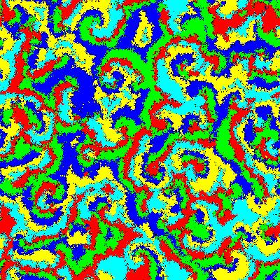
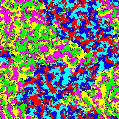
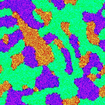
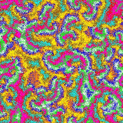
Fig. 1 shows some typical two-dimensional space-time patterns that we aim at predicting with the approach discussed in the following. Whereas snapshot (a) shows an example of a system with spirals where every wavefront contains only one species, panel (b) gives an example of a coarsening process with two types of domains where inside every domain spirals are formed, thus yielding non-trivial dynamics inside the coarsening domains. Example (c) reveals a coarsening process where every domain is formed by an alliance of mutually neutral species. Finally, snapshot (d) shows a case of fuzzy spirals due to the mixing of different species inside the waves.
(a) (b)
(c) (d)
In order to focus our discussion we consider in the following systems of species in two space dimensions where individuals of different species have mutual predator-prey interactions, give birth to off-springs, and are mobile. For our method the details of the implementation of these interactions do not matter, with the exception that the predation-prey interactions should be binary, i.e. at any given event one predator consumes one prey. For the examples in Fig. 1 as well as for the more complicated cases discussed later we consider the following general interaction scheme ( denotes a member of species and is an empty site):
| (1) | |||||
| (2) | |||||
| (3) | |||||
| (4) |
where every lattice site can be occupied by at most one individual, whereas reactions between different individuals only occur when they are at neighboring sites. Our approach remains valid when considering in addition self-predation. The model parameters , , , and are the rates at which these reactions take place. For the examples included in this paper, predation and swapping rates are always considered to be independent of the prey, i.e. and . The separation of the predation and birth events is needed for the formation of spirals as those shown in Fig. 1, but is otherwise not relevant in order to establish the relationships between species. We also allow for various ways of mobility (swapping of individuals on neighboring sites (3) or diffusion by jumping to empty sites (4)), in order to be as general as possible.
The reaction scheme (1)-(2) contains many known situations as for example the cyclic species Lotka-Volterra and May-Leonard models as well as more complicated situations like the models where each species preys on other species in a cyclic way (Roman et al., 2013; Mowlaei et al., 2014). Whereas the examples shown in Fig. 1 are those of models with symmetric rates (hence we can drop the labels , for the rates, see the figure caption), more general cases will be discussed below.
The matrix approach discussed in the following is valid for rather general predator-prey networks, provided that no interactions of higher order than second order are present. We assume that the species network gives rise to a unique partition of the species into domains. While we have not encountered a case where this assumption is not fulfilled, we can not exclude that there exist networks of species that exhibit in presence of noise two non-isomorphic partitions of species into domains. For the cases used to illustrate our approach, we consider rates for which none of the species go extinct before the quasi-steady state of the dynamics is reached, i.e. the time scale on which the species are forming alliances and domains is shorter than the extinction time for any of the species. Notably this requires that the diffusion and mobility rates are not too high so as to induce rapid extinction of the species, but are still large enough to allow the formation of species alliances.
3 Matrix approach
The predation scheme (1) can be represented by a graph where one connects species and by a directed edge if preys on . The scheme can also be encoded in the adjacency matrix where the element if preys on and 0 otherwise. The square of the adjacency matrix contains information about preferred partnership formations based on the maximum protection a species can enjoy while being close to some other species. Indeed, the element counts the number of directed paths of length 2 from vertex to vertex , i.e. the number of paths of the form where is a vertex different from and . Following the maxim that ”the enemy of my enemy is my friend,” species wants to be in close proximity to that species that attacks most of its predators. Mathematically, this preferred partner of is obtained from the condition .
Of course, a given species does not want to undergo a close partnership with one of its predators. Adding this important information yields the alliance matrix whose elements provide information on the best possible allies for each species :
| (5) |
where . The first condition selects those species that are preferred partners of as they provide the best protection by attacking the largest number of its predators, whereas the second condition makes sure that is not itself a predator of , yielding a matrix with elements for the best possible allies of species and zero otherwise.
In order to fully understand space-time patterns as those shown in Fig. 1, one needs to further distinguish between preferred allies of species that are hunted by species and preferred allies towards which species has a neutral approach. This information is encoded by the two matrices (prey-allies) and (neutral allies) with elements
| (6) | |||||
| (7) |
with the binary operators AND () and NOT ().
The two matrices and allow to understand (and predict) many of the space-time patterns that can emerge in predator-prey systems governed by the reactions (1)-(2). A matrix element means that species seeks the protection of species , while at the same time preying on species . As a result single species waves will form where a wave containing individuals of species will follow one formed by species . On the other hand represents non-aggressive coexistence where species is protected by a neutral species (i.e. does not prey on ). As a result will mix with in order to enjoy the enhanced protection by its preferred ally. If , then the two mutually neutral partners will form neutral domains and protect each other.
Inspection of Fig. 1d reveals a case that is not yet covered by the matrices given above, namely that of ’fuzzy’ waves where three species mix to some degree. Consider three given species , , and . The above situation is encountered when species and are mutually neutral and species and are mutually neutral, while at the same time species preys on species . This means that the following conditions have to be fulfilled simultaneously: , , and . As a result, chases species while both mix with the intermediate species , giving fuzzy looking waves as those seen in Fig. 1d. Defining the matrix elements of a matrix as
| (8) |
with for and zero otherwise, we have that if acts as a neutral intermediary between species and some other species, whereas otherwise.
4 Examples
Let us first look at the four cyclic games of Fig. 1 in order to see how to work with the different matrices.
For the game shown in Fig. 1a the relevant matrix is
| (9) |
whereas . We readily obtain from the prey-allies matrix that species 1 wants to ally with its prey species 2, species 2 wants to ally with its species 3, etc. This yields single species spirals where the species follow each other in the order .
The in Fig. 1b is characterized by a similar looking matrix
| (10) |
where again . This time, however, two family of spirals (or teams) are formed, one with the ordering , the other with the ordering . As every member in a team has both a prey and a predator in the other team, these two family of spirals compete against each other, which yields a coarsening process with a three-species rock-paper-scissors game within each domain.
The case of Fig. 1c is a case where the prey-allies matrix vanishes whereas the neutral allies matrix is non-zero:
| (11) |
Inspection of reveals the formation of three teams composed of two mutually neutral species (1 and 4, 2 and 5, 3 and 6), resulting in a coarsening process with three different types of domains.
Finally, the game in Fig. 1d provides us with an example where both and are non-zero:
| (12) |
whereas . It follows from this that species 5, which is the preferred ally of species 1, acts as an intermediary between species 1 and 9. As species 9 preys on species 1, this yields a wavefront of the type where indicates a neutral intermediary. As this happens in a cyclic way, one observes the emergence of fuzzy spirals, with the ordering .
Let us now look at the two more involved examples shown in Figs. 2 and 3 where the interaction scheme is no longer cyclic.
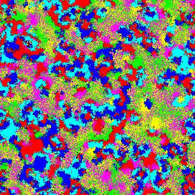
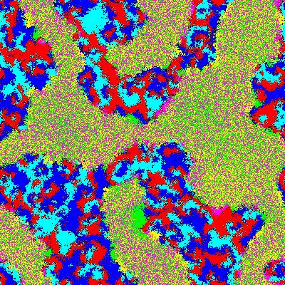
The snapshots in Fig. 2 result from a six-species model with an interaction scheme described by the matrix
| (13) |
and rates given by
| (14) |
Following the construction explained above, we get the matrices
| (15) |
which, together with the fact that , allow us to predict the alliances and space-time pattern appearing in this system. In the present case, both the prey-allies and neutral allies matrices are non-zero, so that we can expect the formation of both neutral alliances as well as of alliances where the partners remain in a predator-prey relationship. Indeed, from the matrix we obtain that species 1, 3, and 5 form a three-species cyclic game that results in the formation of compact wavefronts with the following ordering of the species: . On the other hand, from the matrix follows that the species 2, 4, and 6 form a neutral alliance. As a result, two types of domains should form, one composed of three neutral partners and one composed of three partners that undergo a cyclic rock-paper-scissors game, resulting in a coarsening process with different internal dynamics inside the domains.
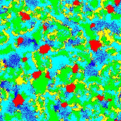
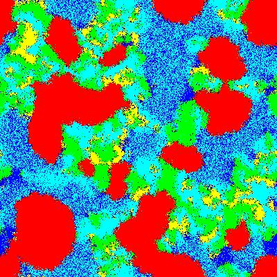
The five-species model shown in Fig. 3 is defined by the adjacency matrix
| (16) |
For the time evolution shown in Fig. 3 we used the rates
| (17) |
From we readily obtain
| (18) |
whereas (i.e. no fuzzy wavefronts are formed). The matrices immediately yield all the relevant information regarding the partnerships forming in this system. As , species 1 wants to self-segregate, which is a direct consequence of the fact that all the other species are both its predators and preys. The neutral allies matrix also indicates that species 3 and 5 form a neutral alliance, in order to fight off their corresponding predators. Finally, the prey-allies matrix reveals that the three species 2, 4, and 5 tend to form an active three-species alliance with the following ordering of the wave fronts: . Our method therefore predicts the formation of three types of domains (pure species 1 domains, domains of the neutral alliance between species 3 and 5, as well as domains where species 2, 4, and 5 undergo a cyclic game), where, remarkably, species 5 is involved in two different alliances. All these predictions are indeed verified when inspecting the snapshots in Fig. 3.
Knowing the partnerships and the resulting space-time pattern is an important step in order to better understand the fate of an ecology. This alone, though, is not enough to predict whether a given species will go extinct, as the survival of a species also depends on the rates of its interactions with the other species. The reliability of our predictions at least for the model with symmetric rates is confirmed via exact agreement with the theoretical predictions in (Mowlaei et al., 2014) obtained using the complex Ginzburg Landau approach. Comprehensive numerical studies are required to fully understand the parameter regimes for which the presented ad-hoc methods are valid. We leave such calculations for future investigations.
5 Summary
We have presented a theoretical approach that allows to predict partnership formation and emerging space-time patterns in many-species food networks. While our emphasis was on predator-prey systems, the proposed use of various matrices, derived from the adjacency matrix, to understand alliances and spatio-temporal pattern formation can be straightforwardly expanded to other systems, ranging from ecology to social sciences (Maynard Smith, 1982; Hofbauer and Sigmund, 1998; Nowak, 2006; Hauert et al., 2002; Gokhale and Traulsen, 2014), governed by binary interactions between different ’species’.
Acknowledgements
M.P. thanks the Galileo Galilei
Institute for Theoretical Physics for the hospitality and
the INFN for partial support during the completion of
this work.
Funding: This work is supported by the US National
Science Foundation through grant DMR-1205309.
References
- Adamson and Morozov (2012) Adamson, M. W., Morozov, A. Y., 2012. Revising the role of species mobility in maintaining biodiversity in communities with cyclic competition. Bull. Math. Biol. 74, 2004-2031.
- Avelino et al. (2012a) Avelino, P. P., Bazeia, D., Losano, L., Menezes, J., 2012. von Neummann’s and related scaling laws in rock-paper-scissors-type games. Phys. Rev. E 86, 031119.
- Avelino et al. (2012b) Avelino, P. P., Bazeia, D., Losano, L., Menezes, J., Oliveira, B. F., 2012. Junctions and spiral patterns in generalized rock-paper-scissors models. Phys. Rev. E 86, 036112.
- Avelino et al. (2014a) Avelino, P. P., Bazeia, D., Menezes, J., Oliveira, B. F., 2014a. String networks in Lotka-Volterra competition models. Phys. Lett. A 378, 393-397.
- Avelino et al. (2014b) Avelino, P. P., Bazeia, D., Losano, L., Menezes, J., Oliveira, B. F., 2014b. Interfaces with internal structures in generalized rock-paper-scissors models. Phys. Rev. E 89, 042710.
- Cheng et al. (2014) Cheng, H., Yao, N., Huang, Z. G., Park, J., Do, Y., Lai, Y.-C., 2014. Mesoscopic interactions and species coexistence in evolutionary game dynamics of cyclic competitions. Sci. Rep. 4, 7486.
- Daly et al. (2015) Daly, A. J., Baetens, J. M., De Baets, B., 2015. The impact of initial evenness on biodiversity maintenance for a four-species in silico bacterial community. J. Theor. Biol. 387, 189-205.
- Dobrinevski et al. (2014) Dobrinevski, A., Alava, M., Reichenbach, T., Frey, E., 2014. Mobility-dependent selection of competing strategy associations. Phys. Rev E 89, 012721.
- Frey (2010) Frey, E., 2010. Evolutionary game theory: Theoretical concepts and applications to microbial communities. Physica A 389, 4265-4298.
- Gokhale and Traulsen (2014) Gokhale, C. S., Traulsen, A., 2014. Evolutionary multiplayer games. Dyn. Games Appl. 4, 468-488.
- Gros̆elj et al. (2015) Gros̆elj, D., Jenko, F., Frey, E., 2015. How turbulence regulates biodiversity in systems with cyclic competition. Phys. Rev. E 91, 033009.
- Guisoni et al. (2013) Guisoni, N. C., Loscar, E. S., Girardi, M., 2013. Phase diagram of a cyclic predator-prey model with neutral-pair exchange. Phys. Rev. E 88, 022133.
- Hauert et al. (2002) Hauert, C., De Monte, S., Hofbauer, J., Sigmund, K., 2002. Volunteering as Red Queen mechanism for cooperation in Public Goods game. Science 296, 1129-1132.
- He et al. (2010) He, Q., Mobilia, M., Täuber, U. C., 2010. Spatial rock-paper-scissors models with inhomogeneous reaction rates. Phys. Rev. E 82, 051909.
- He et al. (2011) He, Q., Mobilia, M., Täuber, U. C., 2011. Coexistence in the two-dimensional May-Leonard model with random rates. Eur. Phys. J. B 82, 97-105.
- He et al. (2012) He, Q., Täuber, U. C., Zia, R. K. P., 2012. On the relationship between cyclic and hierarchical three-species predator-prey systems and the two-species Lotka-Volterra model. Eur. Phys. J. B 85, 141.
- Hofbauer and Sigmund (1998) Hofbauer, J., Sigmund, K., 1998. Evolutionary games and population dynamics. Cambridge University Press, Cambridge, England.
- Intoy and Pleimling (2013) Intoy, B., Pleimling, M., 2013. Extinction in four species cyclic competition. J. Stat. Mech. P08011.
- Intoy and Pleimling (2015) Intoy, B., Pleimling, M., 2015. Synchronization and extinction in cyclic games with mixed strategies. Phys. Rev. E 91, 052135.
- Jiang et al. (2011) Jiang, L. L., Zhou, T., Perc, M., Wang, B. H., 2011. Effects of competition on pattern formation in the rock-paper-scissors game. Phys. Rev. E 84, 021912.
- Jiang et al. (2012) Jiang, L.-L., Wang, W.-X., Lai, Y.-C., Ni, X., 2012. Multi-armed spirals and multi-pairs antispirals in spatial rock-paper-scissors games. Phys. Lett. A 376, 2292-2297.
- Juul et al. (2012) Juul, J., Sneppen, K., Mathiesen, J., 2012. Clonal selection prevents tragedy of the commons when neighbors compete in a rock-paper-scissors game. Phys. Rev. E 85, 061924.
- Juul et al. (2013) Juul, J., Sneppen, K., Mathiesen, J., 2013. Labyrinthine clustering in a spatial rock-paper-scissors ecosystem. Phys. Rev. E 87, 042702.
- Kang et al. (2013) Kang, Y. B., Pan, Q. H., Wang, X. T., Me, H. F., 2013. A golden point rule in rock-paper-scissors-lizard-spock game. Physica A 392, 2652-2659.
- Knebel et al. (2013) Knebel, J., Krüger, T. Weber, M. F., Frey, E., 2013. Coexistence and survival in conservative Lotka-Volterra networks. Phys. Rev. Lett. 110, 168106.
- Lamouroux et al. (2012) Lamouroux, D., Eule, S., Geisel, T., Nagler, J., 2012. Discriminating the effects of spatial extent and population size in cyclic competition among species. Phys. Rev. E 86, 021911.
- Lütz et al. (2013) Lütz, A. F., Risau-Gusman, S., Arenzon, J. J., 2013. Intransitivity and coexistence in four species cyclic games. J. Theor. Biol. 317, 286-292.
- May (1974) May, R. M., 1974. Stability and complexity in model ecosystems. Cambridge University Press, Cambridge, England.
- Maynard Smith (1974) Maynard Smith, J., 1974. Models in ecology. Cambridge University Press, Cambridge, England.
- Maynard Smith (1982) Maynard Smith, J., 1982. Evolution and the theory of games. Cambridge University Press, Cambridge, England.
- Mowlaei et al. (2014) Mowlaei, S., Roman, A., Pleimling, M., 2014. Spirals and coarsening patterns in the competition of many species: A complex Ginzburg-Landau approach. J. Phys. A: Math. Theor. 47, 165001.
- Nahum et al. (2011) Nahum, J. R., Harding, B. N., Kerr, B., 2011. Evolution of restraint in a structured rock-paper-scissors community. Proc. Natl. Acad. Sci. U.S.A. 108, 10831.
- Nowak (2006) Nowak, M. A., 2006. Evolutionary dynamics. Belknap Press, Cambridge, MA.
- Peltomäki and Alava (2008) Peltomäki, M., Alava, M., 2008. Three- and four-state rock-paper-scissors games with diffusion. Phys. Rev. E 78, 031906.
- Perc et al. (2007) Perc, M. Szolnoki, A., Szabó, G., 2007. Cyclical interactions with alliance-specific heterogeneous invasion rates. Phys. Rev. E 75, 052102.
- Provata et al. (1999) Provata A., Nicolis, G., Baras, F., 1999. Oscillatory dynamics in low-dimensional supports: A lattice Lotka-Volterra model. J. Chem. Phys. 110, 8361-8368.
- Reichenbach et al. (2007a) Reichenbach, T., Mobilia, M., Frey, E., 2007a. Mobility promotes and jeopardizes biodiversity in rock-paper-scissors games. Nature 448, 1046-1049.
- Reichenbach et al. (2007b) Reichenbach, T., Mobilia, M., Frey, E., 2007b. Noise and correlations in a spatial population model with cyclic competition. Phys. Rev. Lett. 99, 238105.
- Reichenbach and Frey (2008) Reichenbach, T., Frey, E., 2008. Instability of spatial patterns and its ambiguous impact on species diversity. Phys. Rev. Lett. 101, 058102.
- Roman et al. (2012) Roman, A., Konrad, D., Pleimling, M., 2012. Cyclic competition of four species: domains and interfaces. J. Stat. Mech. P07014.
- Roman et al. (2013) Roman, A., Dasgupta, D., Pleimling, M., 2013. Interplay between partnership formation and competition in generalized May-Leonard games. Phys. Rev. E 87, 032148.
- Rulands et al. (2011) Rulands, S., Reichenbach, T., Frey, E., 2011. Threefold way to extinction in populations of cyclically competing species. J. Stat. Mech. L01003.
- Rulands et al. (2013) Rulands, S., Zielinski, A., Frey, E., 2013. Global attractors and extinction dynamics of cyclically competing species. Phys. Rev. E 87, 052710.
- Rulquin and Arenzon (2014) Rulquin, C., Arenzon, J. J., 2014. Globally synchronized oscillations in complex cyclic games. Phys. Rev. E 89, 032133.
- Shi et al. (2010) Shi, H., Wang, W.-X., Yang, R., Lai Y.-C., 2010. Basins of attraction for species extinction and coexistence in spatial rock-paper-scissors games. Phys. Rev. E 81, 030901(R).
- Schreiber and Killingback (2013) Schreiber, S. J., Killingback, T. P., 2013. Spatial heterogeneity promotes coexistence of rock-paper-scissors metacommunities. Theor. Pop. Biol. 86, 1-11.
- Sole and Basecompte (2006) Sole, R. V., Basecompte, J., 2006. Self-organization in complex ecosystems. Princeton University Press, Princeton, NJ.
- Szabó and Czárán (2001a) Szabó, G., Czárán, T., 2001a. Phase transition in a spatial Lotka-Volterra model. Phys. Rev. E 63, 061904.
- Szabó and Czárán (2001b) Szabó, G., Czárán, T., 2001b. Defensive alliances in spatial models of cyclical population interactions. Phys. Rev. E 64, 042902.
- Szabó and Sznaider (2004) Szabó, G., Sznaider, G. A., 2004. Phase transition and selection in a four-species cyclic predator-prey model. Phys. Rev. E 69, 031911.
- Szabó (2005) Szabó, G., 2005. Competing associations in six-species predator-prey models. J. Phys. A: Math. Gen. 38, 6689-6702.
- Szabó and Fáth (2007) Szabó, G., Fáth, G., 2007. Evolutionary games on graphs. Phys. Rep. 446, 97-216.
- Szabó and Szolnoki (2008) Szabó, G., Szolnoki, A., 2008. Phase transitions induced by variation of invasion rates in spatial cyclic predator-prey models with four or six species. Phys. Rev. E 77, 011906.
- Szabó et al. (2007a) Szabó, G., Szolnoki, A., Sznaider, G. A., 2007a. Segregation process and phase transition in cyclic predator-prey models with an even number of species. Phys. Rev. E 76, 051921.
- Szabó et al. (2007b) Szabó, P. Czárán, T., Szabó, G., 2007b. Competing associations in bacterial warfare with two toxins. J. Theor. Biol. 248, 736-744.
- Szabó et al. (2008) Szabó, G., Szolnoki, A., Borsos, I., 2008. Self-organizing patterns maintained by competing associations in a six-species predator-prey model. Phys. Rev. E 77, 041919.
- Szabó et al. (2015) Szabó, G., Bodó, K. S., Allen, B., Nowak, M. A., 2015. Four classes of interactions for evolutionary games. Phys. Rev. E 92, 022820.
- Szczesny et al. (2013) Szczesny, B., Mobilia, M., Rucklidge, A. M., 2013. When does cyclic dominance lead to stable spiral waves? EPL 102, 28012.
- Szczesny et al. (2014) Szczesny, B., Mobilia, M., Rucklidge, A. M., 2014. Characterization of spiraling patterns in spatial rock-paper-scissors games. Phys. Rev. E 90, 032704.
- Szolnoki and Perc (2015) Szolnoki, A., Perc, M., 2015. Vortices determine the dynamics of biodiversity in cyclical interactions with protection spillovers. New J. Phys. 17, 113033.
- Vandermeer and Yitbarek (2012) Vandermeer, J., Yitbarek, S., 2012. Self-organized spatial pattern determines biodiversity in spatial competition. J. Theor. Biol. 300, 48-56.
- Varga et al. (2014) Varga, L., Vukov, J., Szabó, G., 2014. Self-organizing patterns in an evolutionary rock-paper-scissors game for stochastic synchronized strategy updates. Phys. Rev. E 90, 042920.
- Venkat and Pleimling (2010) Venkat, S., Pleimling, M., 2010. Mobility and asymmetry effects in one-dimensional rock-paper-scissors games. Phys. Rev. E 81, 021917.
- Vukov et al. (2013) Vukov, J., Szolnoki, A., Szabó, G., 2013. Diverging fluctuations in a spatial five-species cyclic dominance game. Phys. Rev. E 88, 022123.
- Wang et al. (2010) Wang, W.-X., Lai Y.-C., Grebogi, C., 2010. Effect of epidemic spreading on species coexistence in spatial rock-paper-scissors games. Phys. Rev. E 81, 046113.
- Wang et al. (2011) Wang, W.-X., Ni, X., Lai Y.-C., Grebogi, C., Pattern formation, synchronization, and outbreak of biodiversity in cyclically competing games. Phys. Rev. E 83, 011917.
- Weber et al. (2014) Weber, M. F., Poxleitner, G., Hebisch, E., Frey, E., Opitz, M., 2014. Chemical warfare and survival strategies in bacterial range expansions. J. R. Soc. Interface 11, 20140172 (2014).
- Winkler et al. (2010) Winkler, A. A., Reichenbach, T., Frey, E., 2010. Coexistence in a one-dimensional cyclic dominance process. Phys. Rev. E 81, 060901(R).