A spatio-temporal stochastic pattern generator
for simulation of uncertainties in geophysical ensemble prediction and ensemble data assimilation

Abstract

A generator of spatio-temporal pseudo-random Gaussian fields that satisfy the “proportionality of scales” property (Tsyroulnikov, 2001) is presented. The generator is based on a third-order in time stochastic differential equation with a pseudo-differential spatial operator defined on a limited area 2D or 3D domain in the Cartesian coordinate system. The generated pseudo-random fields are homogeneous (stationary) and isotropic in space-time (with the scaled vertical and temporal coordinates). The correlation functions in any spatio-temporal direction belong to the Matérn class. The spatio-temporal correlations are non-separable. A spectral-space numerical solver is implemented and accelerated exploiting properties of real-world geophysical fields, in particular, smoothness of their spatial spectra. The generator is designed to create additive or multiplicative, or other spatio-temporal perturbations that represent uncertainties in numerical prediction models in geophysics. The program code of the generator is publicly available.

1 Introduction

1.1 Stochastic dynamic prediction

Since the works of Epstein (1969) and Tatarsky (1969), we know that accounting for the uncertainty in the initial forecast fields can improve weather (and other geophysical) predictions. Assigning a probability distribution for the truth at the start of the forecast (instead of using deterministic initial data) and attempting to advance this distribution in time according to the dynamic (forecast) model is called stochastic dynamic prediction.

The advantage of the stochastic dynamic prediction paradigm is twofold. First, the resulting forecast probability distribution provides a valuable measure of the uncertainty in the prediction, leading to probabilistic forecasting and flow-dependent background-error statistics in data assimilation. Second, for a nonlinear physical model, switching from the deterministic forecast to the mean of the forecast probability distribution improves the mean-square accuracy of the prediction, i.e. can improve the deterministic forecasting.

1.2 Model errors

Since Pitcher (1977), we realize that not only uncertainties in the initial data (analysis errors) matter, forecast model (including boundary conditions) imperfections also play an important role. Simulation of model errors is the subject of this study, so we define them now. Let the forecast model be of the form

$$\frac{{\rm d}{\bf x}}{{\rm d}t}={\bf F}({\bf x}),$$ (1)

where $t$ is time, ${\bf x}$ is the vector that represents the (discretized) state of the system, and ${\bf F}$ is the model (forecast) operator. The imperfection of the model Eq.(1) means that the (appropriately discretized) truth does not exactly satisfy this equation. The discrepancy is called the model error (e.g. Orrell et al., 2001):

$$\boldsymbol{\xi}^{t}={\bf F}({\bf x}^{t})-\frac{{\rm d}{\bf x}^{t}}{{\rm d}t}.$$ (2)

The true model error $\boldsymbol{\xi}^{t}$ is normally unknown. In order to include model errors in the stochastic dynamic prediction paradigm, one models $\boldsymbol{\xi}^{t}(t)$ as a random process, $\boldsymbol{\xi}(t)$, or, in other words, as a spatio-temporal random field $\xi(t,{\bf s})$ (where ${\bf s}$ is the spatial vector). The probability distribution of $\boldsymbol{\xi}(t)$ (in most cases, dependent on the flow) is assumed to be known.

Rearranging the terms in Eq.(2), and replacing the unknown $\boldsymbol{\xi}^{t}$ with its stochastic counterpart $\boldsymbol{\xi}$, we realize that the resulting model of truth is the stochastic dynamic equation

$$\frac{{\rm d}{\bf x}}{{\rm d}t}={\bf F}({\bf x})-\boldsymbol{\xi}.$$ (3)

Thus, the extended stochastic dynamic prediction (or modeling) paradigm requires two input probability distributions (that of initial errors and that of model errors) and aims to transform them to the output (forecast) probability distribution.

1.3 Ensemble prediction

Stochastic dynamic modeling of complex geophysical systems is hampered by their high dimensionality and non-linearity. For realistic models, the output probability distribution is analytically intractable. An affordable approximate solution is provided by the Monte-Carlo method called in geosciences ensemble prediction.

In ensemble prediction, the input uncertainties (i.e. initial and model errors) are represented by simulated pseudo-random draws from the respective probability distributions. A relatively small affordable number of these draws are fed to the forecast model giving rise to an ensemble of predictions (forecasts). If initial and model errors are sampled from the correct respective distributions, then the resulting forecast ensemble members are draws from the correct probability distribution of the truth given all available external data (initial and boundary conditions). This mathematically justifies the ensemble prediction principle. From the practical perspective, members of the forecast ensemble can be interpreted as “potential truths” consistent with all available information.

In what follows, we concentrate on the model error field $\xi(t,{\bf s})$. We briefly review existing models for $\xi(t,{\bf s})$ and then present our stochastic pattern generator, whose goal is to simulate pseudo-random draws of $\xi(t,{\bf s})$ from a meaningful and flexible distribution.

1.4 Practical model error modeling

In meteorology, our knowledge of the actual model error probability distribution is scarce. Justified stochastic model-error models are still to be devised and verified. In the authors’ opinion, the best way to stochastically represent spatio-temporal forecast-model-error fields is to treat each error source separately, so that, say, each physical parametrization is accompanied with a spatio-temporal stochastic model of its uncertainty. Or, even better, to completely switch from deterministic physical parameterizations to stochastic ones. There is a growing number of such developments (see Berner and Coauthors, 2017, for a review), but the problem is so complex that we cannot expect it to be solved in the near future. Its solution is further hampered by the fact that the existing meteorological observations are too scarce and too inaccurate for model errors to be objectively identified by comparison with measurement data with satisfactory accuracy (Tsyrulnikov and Gorin, 2013).

As a result, in meteorology, ad-hoc model-error models are in wide use. The existing approaches can be classified as either non-stochastic or stochastic. Non-stochastic schemes can be multi-model (different ensemble members are generated using different forecast models) or multi-parameterization (each ensemble member is generated using the forecast model with a unique combination of different physical parameterization schemes or their parameters). These techniques are capable of introducing significant diversity in the ensemble (Berner et al., 2011), but the resulting ensemble members cannot be considered as independent and drawn from the same probability distribution (an assumption normally made in using the ensembles). Besides, there are not enough different models and not enough substantially different physical parameterizations to generate large ensembles. Finally, running many forecast models is a technologically very demanding task.

Stochastic approaches, on the contrary, offer the opportunity to generate as many ensemble members taken from the same probability distribution as needed, while working with just one forecast model and one set of physical parameterizations. In atmospheric ensemble prediction and ensemble data assimilation, the most widely used stochastic techniques are SPPT (Stochastic Perturbations of Physical Tendencies, Buizza et al. (1999)), SKEB (Stochastic Kinetic Energy Backscatter scheme, Shutts (2005)), and SPP (Stochastically Perturbed Parameterizations, Christensen et al. (2015), Ollinaho et al. (2017)). In the SPPT, multiplicative perturbations to the tendencies produced by the model’s physical parameterizations are introduced. The multiplier is a spatio-temporal random field centered at 1. In the SKEB, additive perturbations are computed by modulating a spatio-temporal random field by the local kinetic energy dissipation rate. In the SPP, selected parameters of the physical parameterization schemes are perturbed again using a spatio-temporal field, which thus is seen to be needed in all of the above stochastic model error representation schemes. Stochastic parameterization schemes can also demand such fields (e.g. Bengtsson et al., 2013).

1.5 Generation of spatio-temporal random fields

The simplest non-constant pseudo-random field is the white noise, i.e. the uncorrelated in space and time random field. The white noise is the default forcing in stochastic differential equations, e.g. Jazwinski (1970) or Arnold (1974). Its advantage is the complete absence of any spatio-temporal structure, it is a pristine source of stochasticity. But in model-error modeling, this lack of structure precludes its direct use as an additive or multiplicative perturbation field because model errors are related to the weather pattern and so should be correlated (dependent) both in space and time. Tsyrulnikov (2005) showed in a simulation study that model errors can exhibit complicated spatio-temporal behavior.

A correlated pseudo-random spatio-temporal field can be easily computed by generating independent random numbers at points of a coarse spatio-temporal grid and then assigning each of them to all model grid points within the respective coarse-grid cell (Buizza et al., 1999). As a result, the model-grid field becomes correlated in space and time. The decorrelation space and time scales are, obviously, defined by the respective coarse grid spacings (e.g. in Buizza et al. (1999) these were about 1000 km in space and 6 h in time). This technique is extremely simple but it suffers from two flaws.

First, the resulting model-grid field appears to be discontinuous and inhomogeneous. Second, the spatio-temporal structure of the field is not scale dependent, that is, the resulting temporal length scales do not depend on the respective spatial scales. In reality, longer spatial scales “live longer” than shorter spatial scales, which “die out” quicker. This ‘proportionality of scales’ is widespread in geophysical fields (see Tsyroulnikov, 2001, and references therein) and other media, (e.g. Meunier and Zhao, 2009, p.129), so we believe this property should be represented by model-error models. Note also that the “proportionality of scales” is a special case of the non-separability of spatio-temporal covariances. For a critique of simplistic separable space-time covariance models, see Cressie and Huang (1999), Stein (2005), Gneiting et al. (2006), and section 3 below.

Another popular space-time pseudo-random field generation technique employs a spectral transform in space and then imposes independent temporal auto-regressions for the coefficients of the spectral expansion (Berner et al., 2009, Palmer et al., 2009, Charron et al., 2010, Bouttier et al., 2012). This technique is more general and produces homogeneous fields, but the above implementations use the same time scale for all spatial wavenumbers so that there are still no space-time interactions in the generated spatio-temporal fields (though Charron et al. (2010) noted that the decorrelation time scales can be made dependent on the spatial scales and Palmer et al. (2009) allowed for this dependence in their SKEB pattern generator equations).

In this report, we propose and test a spatio-temporal Stochastic (pseudo-random) Pattern Generator (SPG) that accounts for the above “proportionality of scales” and imposes meaningful space-time interactions. The SPG operates on a limited-area domain. It is based on a (spectral-space) solution to a stochastic partial differential equation, more precisely, to a stochastic differential equation in time with a pseudo-differential spatial operator. In what follows, we present the technique, examine properties of the resulting spatio-temporal fields on 2D and 3D spatial domains, describe the numerical scheme, and explore the performance of the SPG. The technique is implemented as a Fortran program freely available from https://github.com/gayfulin/SPG.

2 Model error fields: separability vs. “proportionality of scales”

In this motivational section we show on a simple 1D (in space) example that space-time interactions in the model error random field play a significant role. Specifically, we demonstrate that these interactions determine whether the spatial length scale of the resulting forecast error field grows, in a first approximation, in time or remains constant.

We note that for small enough model error perturbations and small enough lead times, the forecast error due to the accumulated model errors can be approximated by the so-called model-error drift, that is, the time integrated model error: $\bar{\xi}(t,s)=\int_{0}^{t}\xi(t,s)\,{\rm d}t$ (Orrell et al., 2001). Therefore, the methodology in this section is to take two fields, one with separable spatio-temporal correlations and the other with“proportional scales”, integrate them in time, and look at the spatial length scales of the two time integrated random fields.

Theoretically, the time integration reduces (filters out) small-scale-in-time components of the field. As a separable field has no space-time interactions, its time integral should have exactly the same spatial length scale as $\xi(t,s)$. For a proportional-scales field, smaller scales in time are associated with smaller scales in space, so the amount of small spatial scales in the time integrated field should decrease in time leading to an increase in the spatial length scale.

To verify these theoretical conclusions, we set up the following numerical experiment. We considered a 1D domain of size 100 km and the time integration period of 3 h. In this 2D spatio-temporal domain, we introduced a grid with 100 points in space and 100 points in time. On this grid, we simulated two random fields, both with unit variance and exactly the same spatial and temporal exponential correlations. The first field had separable correlations $C_{1}(\Delta t,\Delta s)=\exp(-|\Delta s|/L)\cdot\exp(-|\Delta t|/T)$, whereas the second field had non-separable correlations $C_{2}(\Delta t,\Delta s)=\exp(-\sqrt{(\Delta s/L)^{2}+(\Delta t/T)^{2}}$, which can be shown to satisfy the “proportionality of scales” property. The spatial length scale $L$ was selected in such a way that the spatial correlation function intersects the 0.7 level at the distance of 50 km. The temporal length scale was selected to be equal to $L/U$, where $U=20$ m/s was taken as the characteristic flow velocity. Note that both the separability and the exponential temporal correlation function are what the scale-independent first-order auto-regressions used in Berner et al. (2009), Palmer et al. (2009), Charron et al. (2010), and Bouttier et al. (2012) imply.

Knowing the two correlation functions, we simulated pseudo-random realizations of the two fields (by building the two covariance matrices, computing their square roots, and applying the latter to vectors of independent $N(0,1)$ random variables), see Fig.1.

Figure 1: Simulated spatio-temporal fields. Left:: With separable space-time correlations. Right: With non-separable proportional-scales correlations.

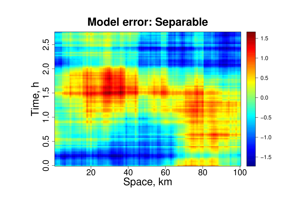
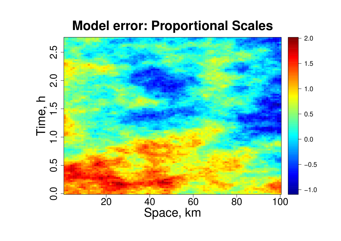
Comparing the two panels of Fig.1, one can see that the two fields look quite differently. Visually, the most striking difference is the lack of isotropy in the separable case. The proportional-scales field looks much more realistic than the separable one.

To get a more objective criterion, we computed the time integrated model error field $\bar{\xi}(t,s)$ (the model error drift, a proxy to the model-error induced forecast error, see above in this section). Figure 2 shows the spatial cross-sections of the arbitrarily chosen realizations of the model error fields (left) and the drift fields (right). The realizations generated by the separable random field model are given in black and the realizations of the proportional-scales field are represented by the red curves.

Figure 2: Spatial cross-sections of the simulated fields. Left:: Model error fields. Right: Time integrated model error fields.

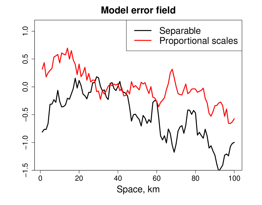
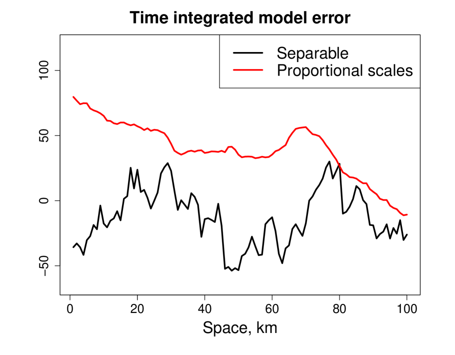
One can see that, indeed, the time integration did not change the spatial structure of the separable field (compare the two black curves in Fig.2, left and right). In contrast, the time integrated proportional-scales field becomes much smoother in space (compare the two red curves in Fig.2, left and right).

Even more objectively, we estimated the spatial micro-scale of the drift $\bar{\xi}(t,s)$. The estimator was $({{\mathsf{Var}}\,\bar{\xi}}/{{\mathsf{Var}}\,\delta\bar{\xi}})^{1/2}\cdot h$, where $\delta\xi$ is the forward finite difference in space, the variance ${\mathsf{Var}}\,$ was estimated by averaging over the space coordinate and over an ensemble of 100 realizations), and $h$ is the spatial mesh size. The resulting spatial micro-scales for the two fields in question are displayed in Fig.3 as functions of time.

Figure 3: Spatial micro-scale as a function of integration time for the two time integrated random fields (separable and proportional-scales).

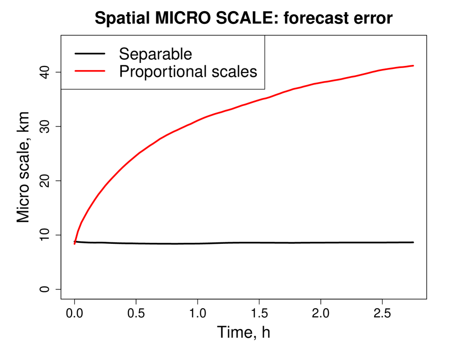
As expected, in the separable case, the spatial micro-scale did not change as a result of the time integration (the flat black line), whereas in the non-separable proportional-scale case, the spatial length scale of the model error drift rapidly grew in time. It is worth emphasizing that in data assimilation, the spatial length scale is a very important attribute of the forecast error field and thus needs to be correctly represented by a forecast (background) ensemble.

Thus, we have shown that the specific type of the spatio-temporal interactions in a model (tendency) error field has important consequences for the spatial structure of the resulting practically relevant forecast error field. We have no evidence on the actual model error spatio-temporal structure, but we know that non-separability and, more specifically, proportionality of scales is ubiquitous in geophysics (Tsyroulnikov, 2001), therefore, we postulate that the SPG should produce proportional-scales fields.

3 SPG: Requirements and approach

The general requirements are:

1. The SPG should produce univariate stationary in time and homogeneous (stationary) and isotropic in space Gaussian pseudo-random fields $\xi(t,{\bf s})$ in 3D and 2D spatial domains.

2. The SPG should be fast enough so that it does not significantly slow down the forecast model computations.

3. The magnitude as well as the spatial and temporal length scales of $\xi(t,{\bf s})$ are to be tunable.

We also impose more specific requirements:

1. The random field $\xi(t,{\bf s})$ should have finite variance and continuous realizations (sample paths).

2. The spatio-temporal covariances should obey the “proportionality of scales” principle: larger (shorter) spatial scales should be associated with larger (shorter) temporal scales (Tsyroulnikov, 2001).

3. The SPG ansatz should be flexible enough to allow for practicable solutions in both physical space and spectral space.

Two comments are in order. Firstly, stationarity, homogeneity, isotropy, and Gaussianity imposed by requirement 1 are just the simplest natural properties of a spatio-temporal random field. The SPG is intended to be used as a building block in practical schemes like the above SPPT, SKEB, SPP, or others. Its role is to be the source of meaningful and easily tunable spatio-temporal stochasticity, whereas physical model error features (flow dependence, non-Gaussianity, etc.) are to be provided by the specific model error modeling scheme on a point-by-point basis.

Secondly, requirement 6 demands an SPG equation to be solvable in physical space as well as in spectral space for the following reasons. All the above mentioned existing pattern generators are spectral space based because this is the simplest way to get a homogeneous and isotropic field in physical space. So, following this path, we would like to have a spectral-space solver. But we envision that a combination of a homogeneous and isotropic spatial structure (provided by the SPG) and point-by-point flow dependent and/or non-Gaussian features (provided by the specific model error modeling scheme) can appear too restrictive in the near future. Specifically, this combination approach cannot produce variable local spatial and temporal length scales if used in schemes like the SKEB or SPP (say, we may wish to reduce the local length scales in meteorologically active areas like cyclones or convective systems). Therefore, we wish the SPG equation to allow for a physical-space solver that would be capable of imposing variable in space and time structures.

As a starting point in the development of the SPG, we select the general class of linear evolutionary stochastic partial differential equations (SPDE). This choice is motivated by the flexibility of this class of spatio-temporal models (e.g. Lindgren et al., 2011). In particular, for an SPDE, it is relatively easy to introduce inhomogeneity (non-stationarity) in space and time as well as local anisotropy—either by changing coefficients of the spatial operator or by changing local properties of the driving noise. One can also produce non-Gaussian fields by making the random forcing non-Gaussian (e.g. Åberg and Podgórski, 2011, Wallin and Bolin, 2015). Physical-space discretizations of SPDEs lead to sparse matrices, which give rise to fast numerical algorithms. If an SPDE has constant coefficients, then it can be efficiently solved using spatial spectral-space expansions.

In this study, we develop the SPG that relies on a spatio-temporal stochastic model with constant coefficients so that both physical-space and spectral-space solvers can be employed. To facilitate the spectral-space solution, the general strategy is to define the SPG model on a standardized spatial domain. The operational pseudo-random fields are then produced by mapping of the generated fields from the standardized domain to the forecast-model domain. In 3D, the standardized spatial domain is chosen to be the unit cube with the periodic boundary conditions in all three dimensions, in other words, the three-dimensional (3D) unit torus. In 2D, the standardized domain is the 2D unit torus. The 3D and 2D cases are distinguished by the dimensionality $d=2$ or $d=3$ in what follows. To simplify the presentation, the default dimensionality will be $d=3$.

4 Tentative first-order SPG model

4.1 Physical-space model

The random field in question $\xi(t,{\bf s})$ is a function of the time coordinate $t$ and the space vector ${\bf s}=(x,y,z)$, where $(x,y,z)$ are the three spatial coordinates. Each of the spatial coordinates belongs to the the unit circle ${\mathbb{S}}^{1}$, so that ${\bf s}$ is on the unit torus $T^{3}={\mathbb{S}}^{1}\times{\mathbb{S}}^{1}\times{\mathbb{S}}^{1}$ (${\mathbb{T}}^{2}$ in the 2D case).

We start with the simplest general form of the first-order Markov model:

$$\frac{\partial\xi(t,{\bf s})}{\partial t}+A\,\xi(t,{\bf s})=\alpha(t,{\bf s}),$$ (4)

where $A$ is the spatial linear operator to be specified and $\alpha$ is the driving noise. $\alpha$ is postulated to be white in space and time; this is done to facilitate a fast numerical solver in physical space as demanded by requirement 6 in section 3 because generation of the white noise is computationally inexpensive (its values on a grid in space and time are just independent Gaussian random variables).

The SPG is required to be fast, so we choose $A$ to be a differential operator (because, as we noted, in this case a physical-space discretization of $A$ gives rise to a very sparse matrix).

Further, since we wish $\xi(t,{\bf s})$ to be homogeneous and isotropic in space, we define $A$ to be a polynomial of the negated spatial Laplacian:

$$A=P(-\Delta)=\sum^{q}_{j=0}c_{j}(-\Delta)^{j},$$ (5)

where $P(x)$ is the polynomial and $q$ its degree (a positive integer). We will refer to $q$ as the spatial order of the SPG model. Note that the negation of the Laplacian is convenient because $(-\Delta)$ is a non-negative definite operator.

The model Eq.(5) appears to be too rich for the purposes of the SPG at the moment, so in what follows we employ an even more reduced (but still quite flexible) form

$$A=P(-\Delta)=\mu(1-\lambda^{2}\Delta)^{q},$$ (6)

where $\mu$ and $\lambda$ are positive real parameters. So, we start with the following SPG equation:

$$\frac{\partial\xi(t,{\bf s})}{\partial t}+\mu(1-\lambda^{2}\Delta)^{q}\,\xi(t,{\bf s})=\alpha(t,{\bf s}).$$ (7)

4.2 Spectral-space model

On the torus ${\mathbb{T}}^{\mathnormal{d}}$, a Fourier series is an expansion in the basis functions $\rm e^{{\mathsf{i}}({\bf k},{\bf s})}\equiv\rm e^{{\mathsf{i}}(\mathnormal{mx+ny+lz})}$, where the wavevector ${\bf k}$ is, for $d=3$, the triple of integer wavenumbers, ${\bf k}=(m,n,l)$. We perform the Fourier decomposition for both $\alpha(t,{\bf s})$ and $\xi(t,{\bf s})$,

$$\alpha(t,{\bf s})=\sum_{{\bf k}\in{\mathbb{Z}}^{d}}\tilde{\alpha}_{\bf k}(t)\rm e^{{\mathsf{i}}({\bf k},{\bf s})}$$ (8)

and

$$\xi(t,{\bf s})=\sum_{{\bf k}\in{\mathbb{Z}}^{d}}\tilde{\xi}_{\bf k}(t)\rm e^{{\mathsf{i}}({\bf k},{\bf s})}$$ (9)

(where ${\mathbb{Z}}$ denotes the set of integer numbers) and substitute these expansions into Eq.(7). From the orthogonality of the basis functions, we obtain that Eq.(7) decouples into the set of ordinary stochastic differential equations (OSDE, e.g. Jazwinski, 1970, Arnold, 1974) in time:

$$\frac{{\rm d}\tilde{\xi}_{\bf k}}{{\rm d}t}+\mu(1+\lambda^{2}{k}^{2})^{q}\,\tilde{\xi}_{\bf k}(t)=\tilde{\alpha}_{\bf k}(t),$$ (10)

where $k=|{\bf k}|=\sqrt{m^{2}+n^{2}+l^{2}}$. The white driving noise $\alpha$ is stationary, hence the spectral-space coefficients $\tilde{\alpha}_{\bf k}(t)$ are probabilistically independent random processes. This is well known for random fields on the $d$-dimensional real space ${\mathbb{R}}^{d}$ (where spectra are continuous), see e.g. Chapter 2 in Adler (1981) or section 8 in Yaglom (1987), and can be directly verified in our case of the fields on the torus (where spectra are discrete). Therefore, for different wavevectors ${\bf k}$, the resulting spectral-space equations are probabilistically completely independent from each other. This greatly simplifies the solution of the SPG equations because instead of handling the complicated SPDE Eq.(7) we have to solve a number of independent simple OSDEs Eq.(10).

Further, from the postulated whiteness of the spatio-temporal random field $\alpha(t,{\bf s})$, all $\tilde{\alpha}_{\bf k}(t)$ are white in time random processes with the same intensity $\sigma$, (Appendix A):

$$\tilde{\alpha}_{\bf k}(t)=\sigma\,\Omega_{\bf k}(t),$$ (11)

where $\Omega_{\bf k}(t)$ are the independent standard white noises, i.e. the derivatives of the independent standard Wiener processes $W_{\bf k}(t)$ such that

$$\Omega_{\bf k}(t){\rm d}t={\rm d}W_{\bf k}(t).$$ (12)

Thus, the first-order SPG model reduces to a series of OSDEs

$${\rm d}\tilde{\xi}_{\bf k}+\mu(1+\lambda^{2}{k}^{2})^{q}\,\tilde{\xi}_{\bf k}\,{{\rm d}t}=\sigma\,{\rm d}W_{\bf k}.$$ (13)

For practical purposes the series is truncated, so that ${\bf k}\equiv(m,n,l)$ is limited: $|m|<m_{\rm max}$, $|n|<n_{\rm max}$, and $|l|<l_{\rm max}$, where $m_{\rm max}$, $n_{\rm max}$, and $l_{\rm max}$ are the truncation limits. If not otherwise stated, all the truncation limits are the same and denoted by $n_{\rm max}$.

4.3 Stationary spectral-space statistics

Equation (13) is a first-order OSDE with constant coefficients sometimes called the Langevin equation (e.g. Arnold (1974) or Jazwinski (1970), Example 4.12). Its generic form is

$${\rm d}\eta+a\eta\,{\rm d}t=\sigma{\rm d}W,$$ (14)

where $\eta(t)$ is the random process in question, $a$ and $\sigma$ are constants, and $W(t)$ is the standard Wiener process. The solution to Eq.(14) is known as the Ornstein-Uhlenbeck random process, whose stationary (steady-state) temporal covariance function is

$$B_{\eta}(t)=\frac{\sigma^{2}}{2a}\,\rm e^{\mathnormal{-a|t|}}$$ (15)

(e.g. Jazwinski, 1970, Example 4.12). From Eq.(15), it is clear that $a$ has the meaning of the inverse temporal length scale $\tau=1/a$.

Now, consider the stationary covariance function of the elementary random process $\tilde{\xi}_{\bf k}(t)$,

$${\mathsf{E}\,}\tilde{\xi}_{\bf k}(t_{0})\cdot\tilde{\xi}_{\bf k}(t_{0}+t)=b_{\bf k}\cdot C_{\bf k}(t),$$ (16)

where $b_{\bf k}$ is the variance and $C_{\bf k}(t)$ the correlation function. According to Eq.(9), $\tilde{\xi}_{\bf k}$ is the spatial spectral component of the random field in question $\xi(t,{\bf s})$. Therefore $b_{\bf k}={\mathsf{Var}}\,\tilde{\xi}_{\bf k}$ is called the spatial spectrum of $\xi(t,{\bf s})$. From Eqs.(13) and (15), we have

$$b_{\bf k}=\frac{\sigma^{2}}{2\mu(1+\lambda^{2}{k}^{2})^{q}}$$ (17)

and $C_{\bf k}(t)=\exp(-{|t|}/{\tau_{\bf k}})$, where

$$\tau_{\bf k}=\frac{1}{\mu(1+\lambda^{2}{k}^{2})^{q}}$$ (18)

is the temporal length scale associated with the spatial wavevector ${\bf k}$.

Note that by the spectrum (e.g. $b_{\bf k}$) we always mean the modal spectrum, i.e. the variance associated with a single basis function (a single wavevector ${\bf k}$); the modal spectrum is not to be confused with the variance (or energy) spectrum.

4.4 Physical-space statistics

In the stationary regime (i.e. after an initial transient period has passed), the above independence of the spectral random processes $\tilde{\xi}_{\bf k}(t)$ (see section 4.2) implies that the random field $\xi(t,{\bf s})$ is spatio-temporally homogeneous, i.e. invariant under shifts in space and time:

$${\mathsf{E}\,}\xi(t,{\bf s})\cdot\overline{\xi(t+\Delta t,{\bf s}+\Delta{\bf s})}=B(\Delta t,\Delta{\bf s}),$$ (19)

where ${\mathsf{E}\,}$ is the expectation operator and

$$B(t,{\bf s})=\sum_{\bf k}b_{\bf k}\,C_{\bf k}(t)\,\rm e^{{\mathsf{i}}({\bf k},{\bf s})}.$$ (20)

In particular, the spatial covariance function is

$$B({\bf s})=B(t=0,{\bf s})=\sum_{\bf k}b_{\bf k}\,\rm e^{{\mathsf{i}}({\bf k},{\bf s})},$$ (21)

where it is seen that the spatial spectrum $b_{\bf k}$ is the Fourier transform of the spatial covariance function $B({\bf s})$.

The temporal covariance function is

$$B({t})=B(t,{\bf s=0})=\sum_{\bf k}b_{\bf k}\,C_{\bf k}(t).$$ (22)

Finally, the variance is

$${\mathsf{Var}}\,\xi=B(t=0,{\bf s=0})=\sum_{\bf k}b_{\bf k}.$$ (23)

4.5 “Proportionality of scales” requires that $q=\frac{1}{2}$

The more precise formulation of the “proportionality of scales” requirement 5 states that for large $k$, the temporal length scale $\tau_{\bf k}$ should be inversely proportional to $k$:

$$\tau_{\bf k}\sim\frac{1}{k}\quad\mbox{as}\quad k\to\infty.$$ (24)

From Eq.(18), this condition entails, importantly, that

$$q=\frac{1}{2}.$$ (25)

Below, we show that the choice $q=\frac{1}{2}$ causes the generated spatio-temporal random fields to possess, besides the “proportionality of scales”, many other nice properties (sections 5.4 and 5.5).

4.6 The spatial operator of order $q=\frac{1}{2}$

The model’s spatial operator $A$ becomes (see Eq.(6))

$$A=\mu({1-\lambda^{2}\Delta})^{\frac{1}{2}}\equiv\mu\sqrt{1-\lambda^{2}\Delta}.$$ (26)

This is a pseudo-differential operator (e.g. Shubin, 1987) with the symbol

$$a({k})=\mu\sqrt{1+\lambda^{2}{k}^{2}},$$ (27)

so that the action of $A$ on the test function $\varphi({\bf s})$ is defined as follows. First, we Fourier transform $\varphi({\bf s})$ getting $\{\tilde{\varphi}_{\bf k}\}$. Then, $\forall{\bf k}\in{\mathbb{Z}}^{d}$, we multiply $\tilde{\varphi}_{\bf k}$ by the symbol $a({k})$. Finally, we perform the backward Fourier transform of $\{a({k})\tilde{\varphi}_{k}\}$ retrieving the result, the function $(A\varphi)({\bf s})$.

So, the action of the above fractional negated and shifted Laplacian on test functions in spectral space is well defined. Importantly, in physical space, the pseudo-differential operator $A$ can be approximated by a discrete-in-space linear operator which is represented by a very sparse matrix, see Appendix B. So, in both spectral space and physical space, the resulting operator $A$ with the fractional degree $q=\frac{1}{2}$ is numerically tractable.

4.7 The first-order model cannot satisfy the SPG requirements

Let us compute ${\mathsf{Var}}\,\xi$ using Eqs.17 and 23. Since $b_{\bf k}$ is a smooth function of the wavevector ${\bf k}$, we may approximate the sum in Eq.23 with the integral (where $b({\bf k})=b_{\bf k}$ for integer wavenumbers), getting

$${\mathsf{Var}}\,\xi\propto\int_{{\mathbb{R}}^{d}}\frac{1}{\sqrt{1+\lambda^{2}{k}^{2}}}\,{\rm d}{\bf k}\propto\int_{{\mathbb{R}}}\frac{k^{d-1}}{\sqrt{1+\lambda^{2}{k}^{2}}}\,{\rm d}k.$$ (28)

To check the convergence of the latter integral in Eq.(28), we examine the $k\to\infty$ limit. For large $k$, the integrand is, obviously, proportional to $k^{d-2}$. As we know, the integral of this kind converges if the integrand decays faster than ${k^{-1-\epsilon}}$ with some $\epsilon>0$. This implies that the integral in Eq.(28) diverges for all $d\geq 1$. In other words, the spectrum Eq.(17) decays too slowly for ${\mathsf{Var}}\,\xi$ to be finite.

So, the SPG model Eq.(7) cannot simultaneously satisfy the proportional-scales requirement 5 (which leads to $q=\frac{1}{2}$) and the finite-variance requirement 4. Consequently, the SPG model is to be somehow changed. The solution is to increase the temporal order of the model.

5 Higher-order in time model

5.1 Formulation

The SPG model of higher temporal order is

$$\left(\frac{\partial}{\partial t}+\mu\sqrt{1-\lambda^{2}\Delta}\right)^{p}\xi(t,{\bf s})=\alpha(t,{\bf s}),$$ (29)

where $p$ is the temporal order of the modified SPG model (a positive integer). In spectral space, the model reads (cf. section 4.2)

$$\left(\frac{{\rm d}}{{\rm d}t}+\mu\sqrt{1+\lambda^{2}k^{2}}\right)^{p}\tilde{\xi}_{\bf k}(t)=\sigma\,\Omega_{\bf k}(t).$$ (30)

In this section, we explore the steady-state statistics of $\xi(t,{\bf s})$ and find out which values of the temporal order $p$ solve the above infinite variance problem.

5.2 Stationary spectral-space statistics

For each ${\bf k}$, Eq.(30) is a $p$th-order in time OSDE. Using Table 3 in Appendix C, we can write down the stationary variance $b_{\bf k}$ and the temporal correlation function $C_{\bf k}(t)$ of the solution to Eq.(30), the process $\tilde{\xi}_{\bf k}(t)$:

$$b_{\bf k}\propto\frac{\sigma^{2}}{\mu^{2p-1}(1+\lambda^{2}{k}^{2})^{p-\frac{1}{2}}}$$ (31)

(where the sign $\propto$ means proportional to) and

$$C_{\bf k}(t)=\left(1+\frac{|t|}{\tau_{\bf k}}+r_{2}\frac{|t|^{2}}{\tau_{\bf k}^{2}}+\dots+r_{p-1}\frac{|t|^{p-1}}{\tau_{\bf k}^{p-1}}\right)\,\rm e^{-\frac{|\mathnormal{t}|}{\tau_{\bf k}}}.$$ (32)

Here $r_{2},\dots,r_{p-1}$ are real numbers (given for $p=1,2,3$ in Table 3, see Appendix C) and $\tau_{\bf k}$ are still defined by Eq.(18). Specifically, for the temporal order $p=3$, we have

$$b_{\bf k}|_{p=3}=\frac{3\sigma^{2}}{16\mu^{5}(1+\lambda^{2}{k}^{2})^{\frac{5}{2}}}$$ (33)

and

$$C_{\bf k}(t)|_{p=3}=\left(1+\frac{|t|}{\tau_{\bf k}}+\frac{1}{3}\,\frac{|t|^{2}}{\tau_{\bf k}^{2}}\right)\,\rm e^{-\frac{|\mathnormal{t}|}{\tau_{\bf k}}}.$$ (34)

As Eq.(18) is unchanged in the higher order model, the “proportionality of scales” condition Eq.(24) is still satisfied. In order to achieve the desired dependency of $\tau_{\bf k}$ not only on $k$ (which we already have from Eq.(18)), but also on $\lambda$ (the greater is $\lambda$ the greater should be $\tau_{\bf k}$), we parameterize $\mu$ as

$$\mu=\frac{U}{\lambda},$$ (35)

where $U>0$ is the velocity-dimensioned tuning parameter. Note that $\lambda$ affects both the spatial length scale of $\xi$ (due to Eq.(31)) and the temporal length scale (thanks to Eq.(18)). In contrast, $U$ affects only the temporal length scale.

5.3 Finite-variance criterion

Substituting $b_{k}$ from Eq.(31) into Eq.(23), approximating the sum over the wavevectors by the integral, and exploiting the isotropy of the integrand yields

$${\mathsf{Var}}\,\xi\approx{\mathsf{const}}\cdot\int_{0}^{\infty}\frac{\sigma^{2}}{(1+\lambda^{2}{k}^{2})^{p-\frac{1}{2}}}\,k^{d-1}\,{\rm d}k,$$ (36)

so that we have ${\mathsf{Var}}\,\xi<\infty$ (requirement 4) whenever

$$p>\frac{d+1}{2}.$$ (37)

5.4 Isotropy

In this section, we show that, remarkably, $q=\frac{1}{2}$ is the unique spatial order for which the field $\xi(t,{\bf s})$ appears to be isotropic in space-time. In particular, the shape of the correlation function is the same in any spatial or temporal or any other direction in the spatio-temporal domain ${\mathbb{T}}^{\mathnormal{d}}\times{\mathbb{R}}$.

5.4.1 Spatial isotropy

We note that the spatial isotropy of the random field $\xi$ is the invariance of its covariance function $B({\bf s})$ under rotations. If we were in ${\mathbb{R}}^{d}$ rather than on ${\mathbb{T}}^{\mathnormal{d}}$, isotropy of $B({\bf s})=B(s)$, where $s=|{\bf s}|$ is the spatial distance, would be equivalent to isotropy of its Fourier transform (spectrum) $b({\bf k})$, so that the latter would be dependent only $k=|{\bf k}|$. On the torus, spectra are discrete, i.e. $m,n,l$ take only integer values, so, strictly speaking, $b_{\bf k}$ cannot be isotropic there. To avoid this technical difficulty, we resort (for the theoretical analysis only) to the device used in sections 4.7 and 5.3, the approximation of a sum over the wavevectors by an integral.

Specifically, we assume that $b_{\bf k}$ is smooth enough (which is tantamount to the assumption that $B({\bf s})$ decays on length scales much smaller than the domain’s extents) for the validity of the approximation

$$B({\bf s})=\sum_{\bf k\in{\mathbb{Z}}^{d}}b_{\bf k}\,\rm e^{{\mathsf{i}}({\bf k},{\bf s})}\approx\int_{{\mathbb{R}}^{d}}b({\bf k})\,\rm e^{{\mathsf{i}}({\bf k},{\bf s})}{\rm d}{\bf k},$$ (38)

where $b({\bf k})$ is a smooth function of the real vector argument ${\bf k}\in{\mathbb{R}}^{d}$ such that $\forall\bf k\in{\mathbb{Z}}^{d},b({\bf k})=b_{\bf k}$. The integral in Eq.(38) with the isotropic $b({\bf k})$, see Eq.(31), can be easily shown to be invariant under rotations of ${\bf s}$. This implies that $B({\bf s})$ and so the random field $\xi$ are indeed approximately spatially isotropic.

In the theoretical analysis in this section, we will rely on the approximation Eq.(38) and thus assume that the “spectral grid” is dense enough for the spatial spectra to be treated as continuous ones.

5.4.2 Isotropy in space-time

Consider the OSDE Eq.(30) in the stationary regime. Following Yaglom (1987, section 8), the stationary random process can be spectrally represented as the stochastic integral

$$\tilde{\xi}_{\bf k}(t)=\int_{{\mathbb{R}}}\rm e^{{\mathsf{i}}\omega\mathnormal{t}}\,Z_{\bf k}({\rm d}\omega),$$ (39)

where $\omega$ is the angular frequency (temporal wavenumber) and $Z$ is the orthogonal stochastic measure such that

$${\mathsf{E}\,}|Z_{\bf k}({\rm d}\omega)|^{2}=b_{\bf k}(\omega)\,{\rm d}\omega,$$ (40)

where $b_{\bf k}(\omega)$ is the spectral density of the process $\tilde{\xi}_{\bf k}(t)$ (i.e. the Fourier transform of its covariance function $b_{\bf k}C_{\bf k}(t)$, see Eq.(16)) and, at the same time, the spatio-temporal spectrum of the field $\xi$. In the spectral expansion of the driving white noise $\Omega_{\bf k}(t)$ (see Eq.(30)),

$$\Omega_{\bf k}(t)=\int_{{\mathbb{R}}}\rm e^{{\mathsf{i}}\omega\mathnormal{t}}\,Z_{\Omega_{\bf k}}({\rm d}\omega),$$ (41)

we have ${\mathsf{E}\,}|Z_{\Omega_{\bf k}}({\rm d}\omega)|^{2}={\mathsf{const}}\cdot{\rm d}\omega$ because the white noise has constant spectral density. Next, we substitute Eqs.(39) and (41) into Eq.(30), getting

$$({\mathsf{i}}\omega+\mu\sqrt{1+\lambda^{2}k^{2}})^{p}Z_{\bf k}({\rm d}\omega)=Z_{\Omega_{\bf k}}({\rm d}\omega).$$ (42)

In this equation, taking expectation of the squared modulus of both sides, recalling that $\mu=U/\lambda$, and introducing the scaled angular frequency $\omega^{\prime}=\omega/U$, we finally obtain

$$b_{\bf k}(\omega^{\prime})\equiv b_{\bf K}\propto\frac{1}{(\lambda^{-2}+(\omega^{\prime})^{2}+k^{2})^{p}}=\frac{1}{(\lambda^{-2}+{\bf K}^{2})^{p}},$$ (43)

where

$${\bf K}=(\ \frac{\omega}{U},{\bf k})\equiv(\frac{\omega}{U},m,n,l)$$ (44)

is the spatio-temporal wavevector.

From Eq.(43), one can see that with the scaled frequency (note that the change $\omega\to\omega/U$ corresponds to the change of the time coordinate $t\to t\cdot U$), the spatio-temporal spectrum $b_{\bf k}(\omega^{\prime})\equiv b_{\bf K}$ becomes isotropic in space-time. This implies that the correlation function of $\xi$ is isotropic in space-time as well (with the scaled time coordinate). Note that this remarkable property can be achieved only with the spatial order $q=\frac{1}{2}$.

It is worth noting that the functional form of the spatio-temporal spectrum Eq.(43) together with the constraint Eq.(37) imply that the conditions of Theorem 3.4.3 in Adler (1981) are satisfied, so that spatio-temporal sample paths of the random field $\xi$ are almost surely continuous, as we demanded in section 3, see requirement 4.

5.5 Spatio-temporal covariances: the Matérn class

The spatio-temporal field satisfying the $p$-th order SPG model Eq.(29) has the spatio-temporal correlation function belonging to the so-called Matérn class of covariance functions (e.g. Stein, 1999, Guttorp and Gneiting, 2006). To see this, we denote

$$\nu=p-\frac{d+1}{2}>0,$$ (45)

where the positivity follows from Eq.(37). Then Eq.(43) rewrites as

$$b_{\bf K}\propto\frac{1}{(\lambda^{-2}+{\bf K}^{2})^{\nu+\frac{d+1}{2}}}.$$ (46)

Note that here $d+1$ is the dimensionality of space-time. Equation (46) indeed presents the spectrum of the Matérn family of correlation functions, see e.g. Eq.(32) in Stein (1999). The respective isotropic correlation function is given by the equation that precedes Eq.(32) in Stein (1999) or by Eq.(1) in Guttorp and Gneiting (2006):

$$B(r)\propto({r}/{\lambda})^{\nu}K_{\nu}({r}/{\lambda}),$$ (47)

where $r=\sqrt{s^{2}+(Ut)^{2}}$ is the distance (in our case, the Euclidean distance in space-time with the coordinates $(x,y,z,Ut)$) and $K_{\nu}$ is the MacDonald function (the modified Bessel function of the second kind).

The Matérn family is often recommended for use in spatial analysis due to its notable flexibility with only two free parameters: $\nu$ and $\lambda$, see e.g. Stein (1999) and Guttorp and Gneiting (2006). Specifically, $\lambda$ controls the length scale, whereas $\nu>0$ determines the degree of smoothness: the higher $\nu$, the smoother the field. Note that the smoothness is understood as the number of the mean-square derivatives of the random field in question. The degree of smoothness depends on the behavior of the correlation function at small distances and manifests itself in field’s realizations as the amount of small-scale noise (for illustration see Appendix D).

Table 1 lists the resulting correlation functions (in any direction in space-time) for several combinations of $d$ and $p$ (see Guttorp and Gneiting, 2006, for details).

Table 1: Spatio-temporal correlation functions $B(r)$ for some plausible combinations of the dimensionality $d$ and the temporal order $p$

$d$	$p$	$\nu=p-\frac{d+1}{2}$	$B(r)$
2	2	$\frac{1}{2}$	$\rm e^{-\frac{\mathnormal{r}}{\lambda}}$
2	3	$\frac{3}{2}$	$(1+\frac{r}{\lambda})\,\rm e^{-\frac{\mathnormal{r}}{\lambda}}$
2	4	$\frac{5}{2}$	$(1+\frac{r}{\lambda}+\frac{1}{3}\left(\frac{r}{\lambda}\right)^{2})\,\rm e^{-\frac{\mathnormal{r}}{\lambda}}$
3	3	$1$	$\frac{r}{\lambda}K_{1}(\frac{r}{\lambda})$

With the fixed $d$, the larger $p$ corresponds, according to Eq.(45), to the larger $\nu$ and so to the smoother in space and time field $\xi$. This can be used to change the degree of smoothness of the generated field by changing the temporal order of the SPG model.

From the constraint Eq.(37), the minimal temporal order $p$ that can be used in both 2D and 3D is equal to 3. This value ${p=3}$ will be used by default in what follows and in the current SPG computer program.

5.6 Spatio-temporal correlation functions: illustrations

Here we show spatial, temporal, and spatio-temporal correlation functions computed using Eq.(47). To make the plots more accessible, it is arbitrarily assumed that the extent of the standardized spatial domain (the torus) in each dimension is 3000 km, so that the distance is measured in kilometers. The default SPG setup parameters are $\lambda=125$ km and $U=20$ m/s.

5.6.1 Spatial correlation functions

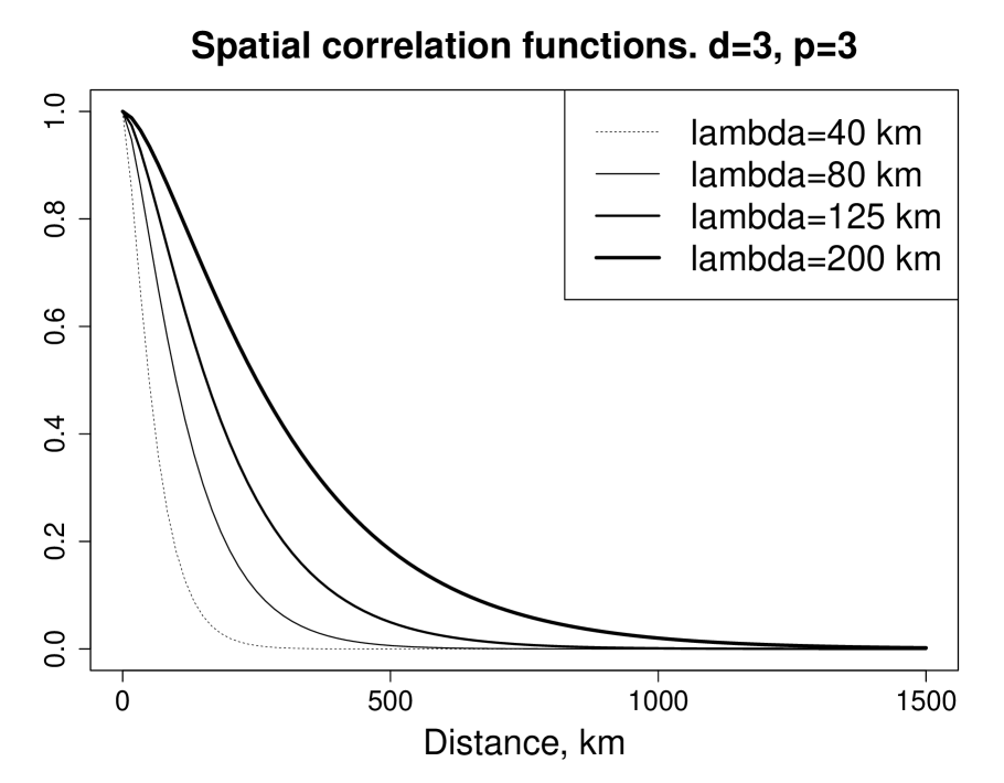
Figure 4 presents the spatial correlation functions for different length scales in 2D and 3D. One can notice, first, that the actual length scale is well controlled by the parameter $\lambda$. Second, it is seen that in 2D (the left panel), where, according to Eq.(45), $\nu=\frac{3}{2}$, the correlation functions are somewhat smoother at the origin than in 3D (the right panel), where $\nu=1$. This is consistent with the above statement that the greater $\nu$ the smoother the field. But in general, the 2D and 3D spatial correlation functions are quite similar.

Figure 4: Spatial correlation functions for $p=3$ in 2D (the left panel) and 3D (the right panel)—for the four spatial length scales indicated in the legend.

5.6.2 Temporal correlation functions

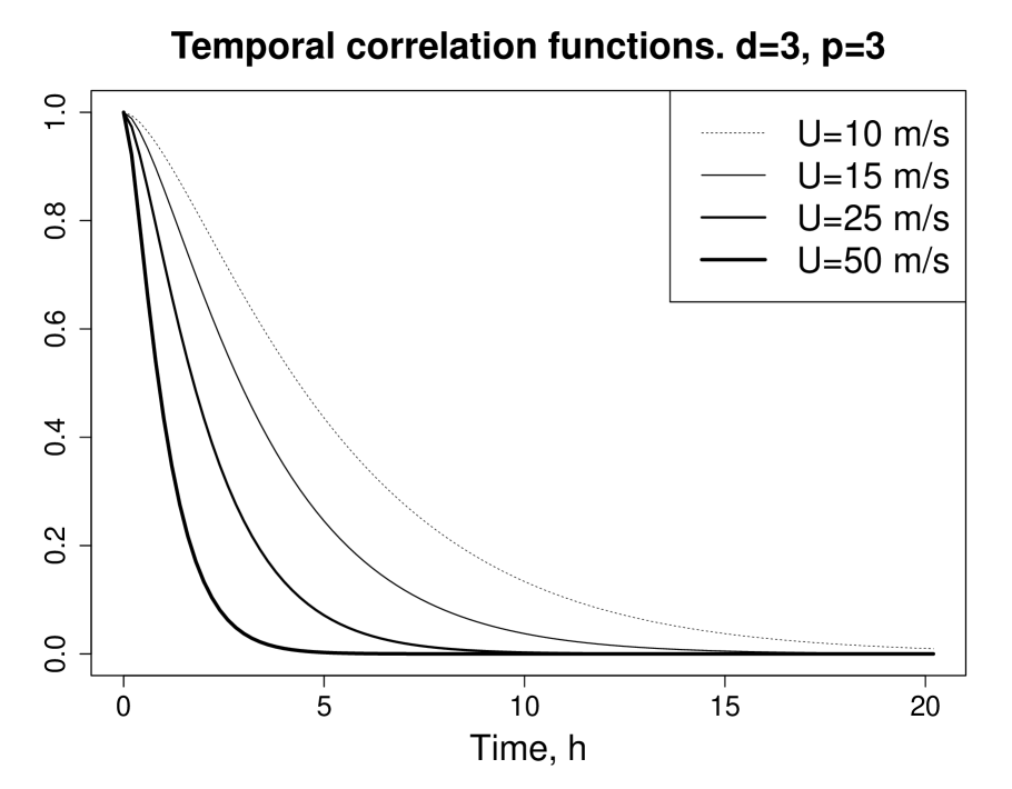
Equation (47) implies that the spatial and temporal correlations have the same shapes. The latter feature is very nice because atmospheric spectra are known to be similar in the spatial and in the temporal domain, e.g. the well-known “-5/3” spectral slope law is observed both in space and time, see e.g. Monin and Yaglom (2013, section 23). So, the SPG does reproduce this observed in the atmosphere similarity of spatial and temporal correlations.

Figure 5 shows the temporal correlation functions for different parameters $U$. Comparing Fig.5 with Fig.4(right), one can observe that the spatial and temporal correlations indeed have the same shape.

Figure 5: Temporal correlation functions in 3D for the four values of $U$ indicated in the legend.

5.6.3 Spatio-temporal correlations

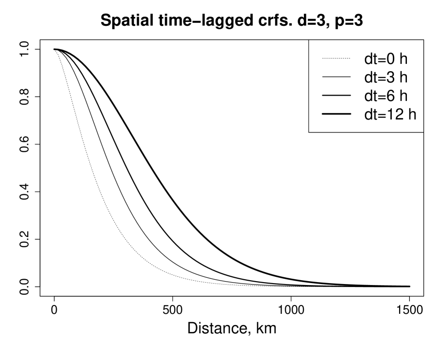
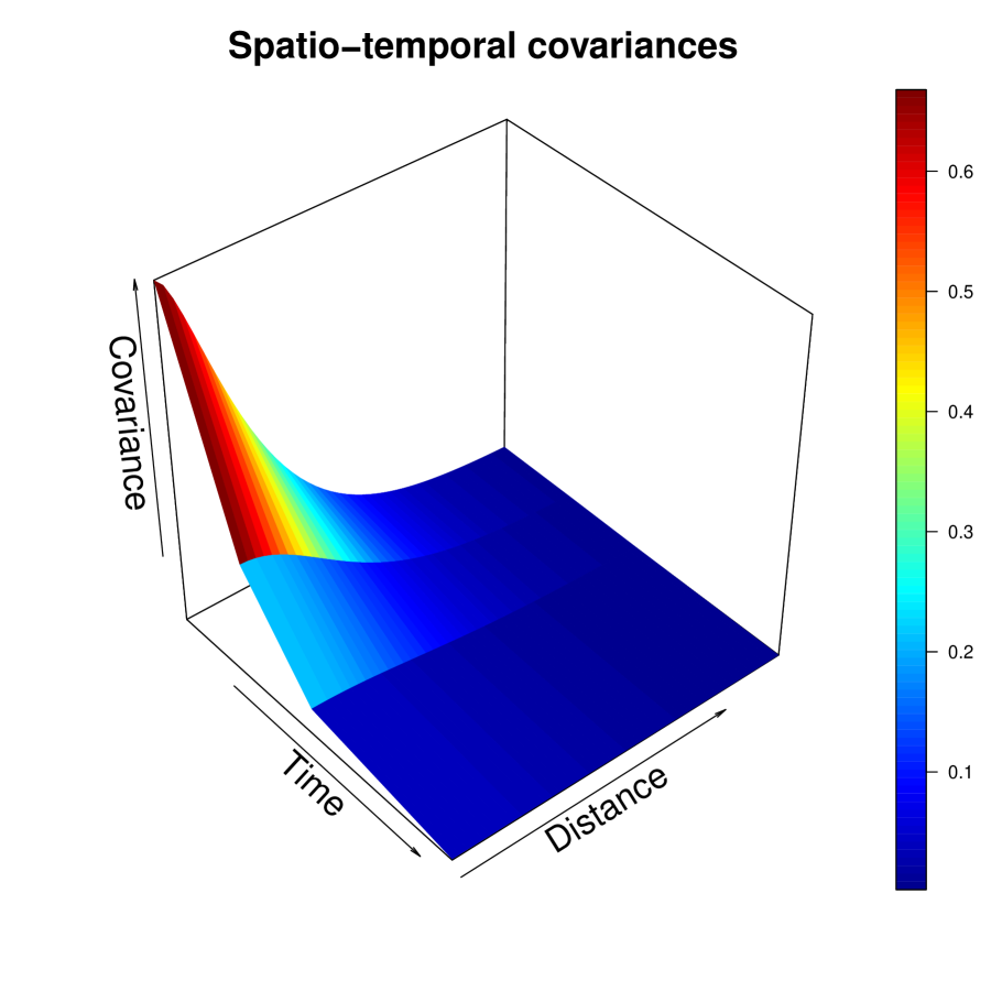
Figure 6 presents the spatial correlation functions for different time lags. Figure 7 displays the spatio-temporal correlation function. In both Fig.6 and Fig.7, another manifestation of the spatio-temporal “proportionality of scales” is seen: the larger the time lag, the broader the spatial correlations. Note that this is consistent with the behavior of the spatio-temporal covariances found by Cressie and Huang (1999, Fig.8) in real-world wind speed data.

Figure 6: Spatial correlation functions in 3D for the four time lags indicated in the legend.

Figure 7: Spatio-temporal SPG covariances.

5.7 Introducing anisotropy in the vertical plane

We have formulated the SPG model under the 3D isotropy assumption. This implies that the ratio of the horizontal length scale to the horizontal domain size is the same as the ratio of the vertical length scale to the vertical domain size. This may be reasonable but, obviously, the independent specification of the horizontal and vertical length scales would be much more flexible. To get this capability, we can employ two equivalent modifications to the SPG model. One approach is to change the radius of the “vertical circle” in the torus from $1$ to the $\delta^{-1}$, where $\delta$ is a positive parameter. Another approach is to replace the Laplacian $\Delta=\frac{\partial^{2}}{\partial x^{2}}+\frac{\partial^{2}}{\partial y^{2}}+\frac{\partial^{2}}{\partial z^{2}}$ by its anisotropic version $\Delta^{\prime}=\frac{\partial^{2}}{\partial x^{2}}+\frac{\partial^{2}}{\partial y^{2}}+\delta^{2}\frac{\partial^{2}}{\partial z^{2}}$. With both approaches, the vertical length scale increases by the factor of $\delta$.

5.8 Preserving isotropy in the horizontal plane for non-square domains

If the size of the domain in physical space in the $x$ direction, $D_{x}$, differs from the domain size in the $y$ direction, $D_{y}$, then mapping from a square SPG domain to the rectangular physical domain would result in an elliptic (also called geometric) anisotropy in the horizontal plane. This undesirable feature can be avoided by replacing $\Delta^{\prime}$ defined in section 5.7 with

$$\Delta_{*}=\frac{\partial^{2}}{\partial x^{2}}+\gamma^{2}\frac{\partial^{2}}{\partial y^{2}}+\delta^{2}\frac{\partial^{2}}{\partial z^{2}},$$ (48)

where $\gamma={D_{x}}/{D_{y}}$. The only change in all the above spectral equations is that the wavenumbers $n$ and $l$ are to be multiplied by $\gamma$ and $\delta$, respectively. The total spatial wavenumber squared $k^{2}$ is to be replaced everywhere by its scaled version

$$k^{2}_{*}=m^{2}+(\gamma n)^{2}+(\delta l)^{2}.$$ (49)

More technically, in our implementation of the SPG, the number of grid points on the torus, $n_{x}^{T},n_{y}^{T},n_{z}^{T}$, differs from that on the physical-space domain, $n_{x},n_{y},n_{z}$, respectively, for two reasons. Firstly, the grid on the torus is defined to have more grid points than in physical space, let us denote them $n_{x}^{+},n_{y}^{+},n_{z}^{+}$. This is done because on the cube with the periodic boundary conditions (i.e. on the torus) the correlations between the opposite sides of the cube are close to 1 due to the periodicity. In order to avoid these spurious correlations on the physical-space domain, we use only part of the grid on the torus (specifically, $n_{x},n_{y},n_{z}$ contiguous grid points) to map the field to the physical-space domain grid point to grid point. Having the user-defined grid sizes in the physical-space domain, $n_{x},n_{y},n_{z}$, we specify the grid sizes on the torus, $n_{x}^{+},n_{y}^{+},n_{z}^{+}$, from the condition that the resulting correlations between the opposite sides of the domain should be less than 0.2. Secondly, we somewhat further increase the number of grid points $n_{x}^{+},n_{y}^{+},n_{z}^{+}$ in order for the final grid sizes on the torus, $n_{x}^{T},n_{y}^{T},n_{z}^{T}$, be multiples of 2,3,5 (as required by the fast Fourier transform software we use).

Then, we find $\gamma$ from the requirement that after the mapping from the torus to the physical-space domain, the length scales of the horizontal function in the $x$ and $y$ directions be the same. It is easy to see that this is the case if

$$\gamma=\frac{n_{x}^{T}}{n_{y}^{T}}.$$ (50)

This device indeed allows to preserve the horizontal isotropy and to change the vertical length scale in a broad range (not shown). We have refrained from introducing this feature to our basic SPG equations for the sake of simplicity of presentation.

5.9 The final formulation of the SPG model

The temporal order of the SPG model is $\boxed{p=3}$. The SPG model is

$$\boxed{\left(\frac{\partial}{\partial t}+\frac{U}{\lambda}\sqrt{1-\lambda^{2}\Delta_{*}}\right)^{3}\xi(t,{\bf s})=\alpha(t,{\bf s})},$$ (51)

where $\alpha(t,{\bf s})$ is the spatio-temporal white noise.

In spectral space, each spectral coefficient $\tilde{\xi}_{\bf k}(t)$ satisfies the equation

$$\boxed{\left(\frac{{\rm d}}{{\rm d}t}+\frac{U}{\lambda}\sqrt{1+\lambda^{2}k_{*}^{2}}\right)^{3}\tilde{\xi}_{\bf k}(t)=\sigma\,\Omega_{\bf k}(t)},$$ (52)

where $\Omega_{\bf k}(t)$ are mutually independent complex standard white noise processes. The intensity of the spatio-temporal white noise $\alpha$ is $(2\pi)^{d/2}\,\sigma$.

6 Time discrete solver for the third-order in time SPG model

In physical space, our final evolutionary model Eq.(29) with $p=3$ can be discretized using the approximation of the operator $\sqrt{1-\lambda^{2}\Delta}$ proposed in Appendix B. The respective physical-space solver looks feasible but we do not examine it in this study. Below, we present our basic spectral-space technique. From this point on, we will consider only the spectral SPG.

6.1 The spectral solver

To numerically integrate the SPG equations in spectral space, we discretize Eq.(30) (with $p=3$) using an implicit scheme. The model operator $(\frac{{\rm d}}{{\rm d}t}+a_{\bf k})^{3}$, where $a_{\bf k}=\frac{U}{\lambda}\sqrt{1+\lambda^{2}k_{*}^{2}}$ and $k_{*}^{2}$ is defined in Eq.(49), is discretized by replacing the time derivative $\frac{{\rm d}}{{\rm d}t}$ with the backward finite difference $\frac{{\cal I-B}}{\Delta t}$, where $\Delta t$ is the time step, ${\cal I}$ is the identity operator, and ${\cal B}$ is the backshift operator. The white noise in the r.h.s. of Eq.(30) is discretized using Eq.(12), where ${\rm d}W_{\bf k}(t)$ is replaced with $\Delta W_{\bf k}(t)=W_{\bf k}(t+\Delta t)-W_{\bf k}(t)$, and simulated as a zero-mean Gaussian random variable with the variance $\Delta t$. As a result, we obtain the time discrete evolution equation

$$\hat{\xi}_{\bf k}(i)=\frac{1}{\varkappa^{3}}\left[3\varkappa^{2}\hat{\xi}_{\bf k}(i-1)-3\varkappa\hat{\xi}_{\bf k}(i-2)+\hat{\xi}_{\bf k}(i-3)+\sigma{\Delta t}^{\frac{5}{2}}\zeta_{{\bf k}t}\right],$$ (53)

where $i=0,1,2,\dots$ denotes the discrete time instance, $\varkappa=1+a_{\bf k}\Delta t$, and $\zeta_{{\bf k}t}\sim CN(0,1)$ are independent complex standard Gaussian pseudo-random variables (for their definition, see Appendix A.6). Note that the solution of the time-discrete Eq.(53) is denoted by the hat, $\hat{\xi}_{\bf k}(i)$, in order to distinguish it from the solution of the time-continuous Eq.(30), which is denoted by the tilde, $\tilde{\xi}_{\bf k}(t)$.

It can be shown that the numerical stability of the scheme Eq.(53) is guaranteed whenever $\varkappa>1$, which is always the case because $a_{\bf k}>0$ (see Eq.(27)).

Note that the derivation of the numerical scheme for a higher-order (i.e. with $p>3$) SPG model is straightforward: one should just raise the difference operator $\frac{{\cal I-B}}{\Delta t}$ to a power higher than 3.

6.2 Correction of spectral variances

Because of discretization errors, the time discrete scheme Eq.(53) gives rise to the steady-state spectral variances $\hat{b}_{\bf k}={\mathsf{Var}}\,\hat{\xi}_{\bf k}(i)$ that are different from the “theoretical” ones, $b_{\bf k}$ (given in Eq.(33)). The idea is to correct (multiply by a number) the solution $\hat{\xi}_{\bf k}(i)$ to Eq.(53) so that the steady-state variance of the corrected $\hat{\xi}_{\bf k}(i)$ be equal to $b_{\bf k}$. To this end, we derive $\hat{b}_{\bf k}$ from Eq.(53) (using Eq.(95) in Appendix E) and then, knowing the “theoretical” $b_{\bf k}$, we introduce the correction coefficients, $\sqrt{b_{\bf k}/\hat{b}_{\bf k}}$, to be applied to $\hat{\xi}_{\bf k}(i)$. This simple device ensures that for any time step, the spatial spectrum and thus the spatial covariances are perfect. But the temporal correlations do depend on the time step, this aspect is discussed below in section 6.4.1.

6.3 “Warm start”: ensuring stationarity from the beginning of the time integration

To start the numerical integration of the third-order scheme Eq.(53), we obviously need three initial conditions. If the integration is the continuation of a previous run, then we just take values of $\hat{\xi}_{\bf k}(i)$ at the last three time instances $i$ from that previous run; this ensures the continuity of the resulting trajectory. If we start a new integration, we have to somehow generate values of ${\bf\hat{\xi}}_{\bf k}(i)$ at $i=1,2,3$, let us denote them here as the vector $\boldsymbol{\xi}^{ini}=({\bf\hat{\xi}}_{\bf k}(1),{\bf\hat{\xi}}_{\bf k}(2),{\bf\hat{\xi}}_{\bf k}(3))^{\top}$. Simplistic choices like specifying zero initial conditions give rise to a substantial initial transient period, which distorts the statistics of the generated field in the short time range.

In order to have the steady-state regime right from the beginning of the time integration and thus avoid the initial transient period completely, we simulate $\boldsymbol{\xi}^{ini}$ as a pseudo-random draw from the multivariate Gaussian distribution with zero mean and the steady-state covariance matrix of $\hat{\xi}_{\bf k}(i)$. In Appendix E, we derive the components of this $3\times 3$ matrix, namely, its diagonal elements (all equal to the steady-state variance), see Eq.(95), and the lag-1 and lag-2 covariances, see Eq.(96).

6.4 Computational efficiency

In this subsection, we describe two techniques that allow us to significantly decrease the computational cost of running the spectral SPG.

6.4.1 Making the time step $\Delta t$ dependent on the spatial wavevector ${\bf k}$

For an ordinary differential equation, the accuracy of a finite-difference scheme depends on the time step. More precisely, it depends on the ratio of the time step $\Delta t$ to the temporal length scale $\tau$ of the process in question. For high accuracy, $\Delta t\ll\tau$ is needed.

In our problem, $\tau_{\bf k}$ decays with the total scaled wavenumber $k_{*}$, see Eqs.(18), (24), and (49). This implies that for higher $k_{*}$, smaller time steps are needed. To maintain the accuracy across the wavenumber spectrum, we choose the time step to be a portion of the time scale:

$$(\Delta t)_{\bf k}=\beta\tau_{\bf k}.$$ (54)

The less $\beta$, the more accurate and, at the same time, more time consuming the numerical integration scheme is.

We note that in atmospheric spectra, small scales have, normally, much less variance (energy) than large scales. But with the constant $\beta$, the computational time would be, on the contrary, spent predominantly on high wavenumbers (because the latter require a smaller time step and are much more abundant in 3D or 2D). So, to save computer time whilst ensuring reasonable overall (i.e. for the whole range of wavenumbers) accuracy, we specify $\beta$ to be wavenumber dependent (growing with the wavenumber) in the following ad-hoc way:

$$\beta_{\bf k}=\beta_{\rm min}+(\beta_{\rm max}-\beta_{\rm min})\left(\frac{k_{*}}{\max k_{*}}\right)^{2},$$ (55)

where $\beta_{\rm min}$ and $\beta_{\rm max}$ are the tunable parameters. The choice of the “optimal” $\beta_{\rm min}$ and $\beta_{\rm max}$ is discussed just below in section 6.4.2.

6.4.2 Introduction of a coarse grid in spectral space

Here we propose another technique to reduce the computational cost of the spectral solver. The technique exploits the smoothness of the SPG spectrum $b_{\bf k}$ Eq.(33). This smoothness allows us to introduce a coarse grid in spectral space and save a lot of computer time by performing the integration of the time discrete spectral OSDEs Eq.(53) only for those wavevectors that belong to the coarse grid. The spectral coefficients $\hat{\xi}_{\bf k}(i)$ are then interpolated from the coarse grid to the dense (full) grid in spectral space.

The latter interpolation would introduce correlations between different spectral coefficients $\hat{\xi}_{\bf k}(i)$, which would destroy the spatial homogeneity. In order to avoid this, we employ a device used to generate so-called surrogate time series (Theiler et al., 1992, section 2.4.1). At each $t$, we multiply the interpolated (i.e. dense-grid) $\hat{\xi}_{\bf k}(i)$ by $\rm e^{{\mathsf{i}}\theta_{\bf k}}$, where $\theta_{\bf k}$ are independent random phases, i.e. independent for different ${\bf k}$ random variables uniformly distributed on the segment $[0,2\pi]$. It can be easily seen that this multiplication removes any correlation between the spectral coefficients.

Note also that the random phase rotation does not destroy the Gaussianity because $\hat{\xi}_{\bf k}(i)$ are complex circularly-symmetric random variables with uniformly distributed and independent of $|\hat{\xi}_{\bf k}(i)|$ arguments (phases) (e.g. Tse and Viswanath, 2005, section A.1.3).

In order to preserve the temporal correlations, we keep the set of $\theta_{\bf k}$ constant during the SPG-model time integration.

The exact spectrum $b_{\bf k}$ after the trilinear (bilinear in 2D) interpolation of $\hat{\xi}_{\bf k}(i)$ from the coarse to the full spectral grid is imposed in a way similar to that described in section 6.2 as follows. At any time instance when we wish to compute the physical space field, for each ${\bf k}$ on the full spectral grid, the linearly interpolated value $\check{\xi}_{\bf k}$ is the linear combination of the closest coarse-grid points ${\bf k}_{j}$:

$$\check{\xi}_{\bf k}=\sum_{j=1}^{2^{d}}w_{j}\,\hat{\xi}_{{\bf k}_{j}}$$ (56)

where $\check{}$ denotes the interpolated value and $w_{j}$ is the interpolation weight (note that the set of the closest coarse-grid points ${\bf k}_{j}$ depends, obviously, on ${\bf k}$). In Eq.(56), the coarse-grid variances ${\mathsf{Var}}\,\hat{\xi}_{{\bf k}_{j}}={b}_{{\bf k}_{j}}$ are known for all ${\bf k}_{j}$ from the spectrum $\{b_{\bf k}\}$, see Eqs.(31) or (33). Therefore, we can find ${\mathsf{Var}}\,\check{\xi}_{\bf k}=\sum_{j}w_{j}^{2}\,b_{{\bf k}_{j}}$. Besides, we know which variance $\check{\xi}_{\bf k}$ should have on the fine grid, namely $b_{\bf k}$. So, we normalize $\check{\xi}_{\bf k}$ by multiplying it by $\sqrt{b_{\bf k}/({\mathsf{Var}}\,\check{\xi}_{\bf k})}$, thus imposing the exact spatial spectrum for all ${\bf k}$.

Technically, the 3D coarse spectral grid is the direct product of three 1D grids. Any of the (non-uniform) 1D coarse grids is specified as follows. Its $j$th point is located at the fine-grid wavenumber $n_{j}$, which equals $j$ for $|j|\leq n_{0}$ (where $n_{0}$ is an integer) and equals the closest integer to $n_{0}(1+\varepsilon)^{|j|-n_{0}}$ for $|j|>n_{0}$. Here, $\varepsilon$ is a tunable small positive number. In the below numerical experiments, the coarse-grid parameters were $n_{0}=20$ and $\varepsilon=0.2$, which resulted in the following positive 1D coarse-grid points: 0 1 2 3 …19 20 24 29 35 42 50 60 72 86 103 124 150 (the 1D grid extent was 300 points and, correspondingly, the maximal wavenumber was 150).

6.4.3 Numerical acceleration: results

As the two above acceleration techniques guarantee that the spatial spectrum is always precise, we tested how these techniques impacted the temporal correlations and what was the speedup. We performed a numerical experiment with the 2D SPG on the grid with $300\times 300$ points, the mesh size $h=7$ km, and the setup parameters $\lambda=80$ km, $U=10$ m/s, and $\delta=\gamma=1$. The time interval $\Delta t_{\rm FFT}$ between the successive backward Fourier transforms determines the effective resolution of the generated field in time. To make the temporal resolution consistent with the spatial resolution, we selected $\Delta t_{\rm FFT}$ close to $h/U$, namely, $\Delta t_{\rm FFT}=15$ min. The computations were performed on a single CPU.

The results are presented in Table 2. We compared the non-accelerated scheme with the constant $\beta=0.1$ and without the sparse spectral grid (the second row) and the accelerated scheme with $\beta_{\rm min}=0.15$, $\beta_{\rm max}=3$, and with the sparse spectral grid (the third row). From column 2, it is seen that the combined effect of the two numerical acceleration techniques on the cost of the spectral-space computations (see column 2) was dramatic: the speedup was 66 times as compared to the non-accelerated scheme. The contributions of the two above numerical acceleration techniques to the spectral-space speedup were comparable in magnitude (not shown). Most importantly, this spectral-space speedup was achieved at the very little cost: the temporal length scale $T_{0.5}$ (defined as the time shift at which the correlation function first intersects the 0.5 level) was distorted by only 4 % w.r.t. the theoretical model (column 6). Note, however, that the cost of the interpolation from the sparse spectral grid (column 3) and of the discrete backward Fourier transform (column 4) reduced the total speedup of the 2D SPG to 14 times (see column 5).

Table 2: CPU times of 2D SPG computations per 1 h of SPG model time and the relative error in the temporal length scale $T_{0.5}$.

Accelerators	CPU spec.	CPU interp.	CPU FFT	Speedup	Rel.err. $T_{0.5}$
NO	0.66	0	0.027	1	3 %
YES	0.010	0.012	0.027	14	4 %

Spec. stands for spectral-space, interp. means interpolation from the sparse spectral grid, and FFT is the fast Fourier transform.

In 3D, the SPG operating on the spatial grid with $300\times 300\times 64$ points, took 40-70 times more CPU time as compared to the above 2D case, with the accuracy being similar to that indicated in Table 2 (not shown). The total speedup was only 8 times due to an increased share of the Fourier transform.

6.5 Examples of the SPG fields

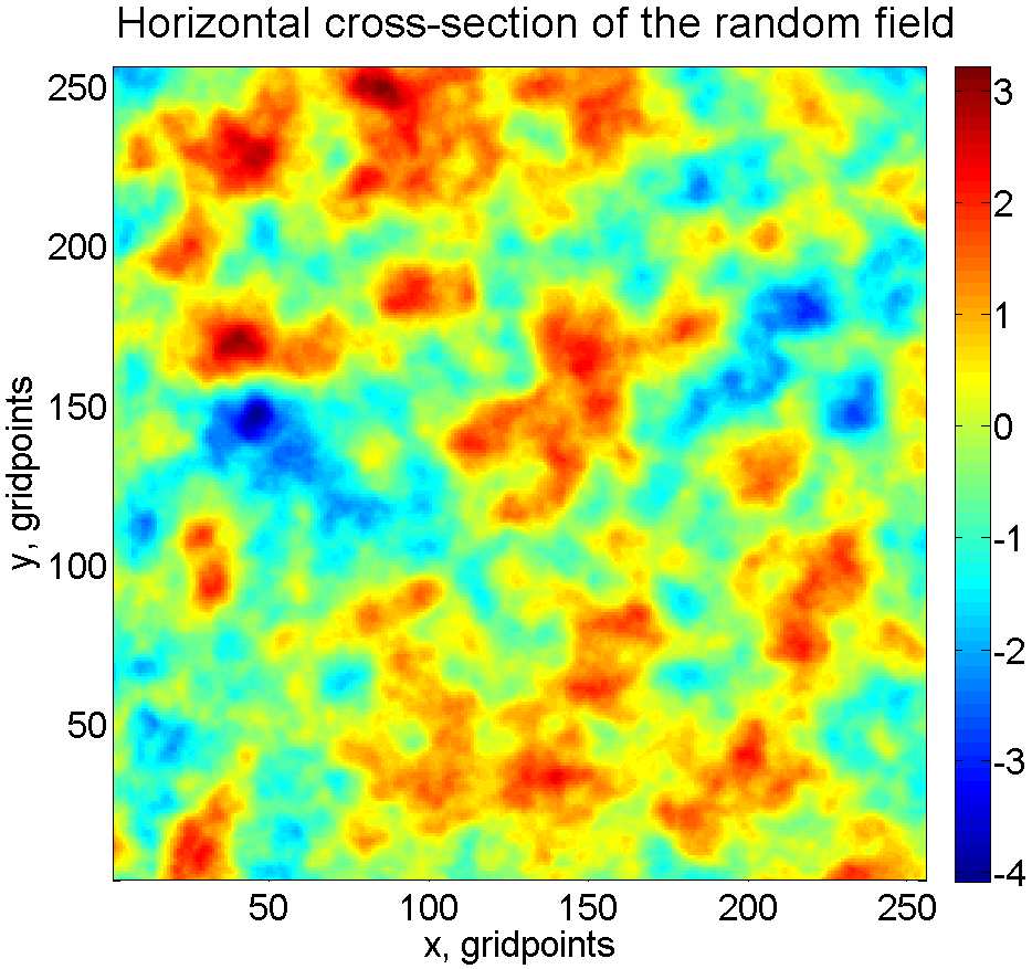
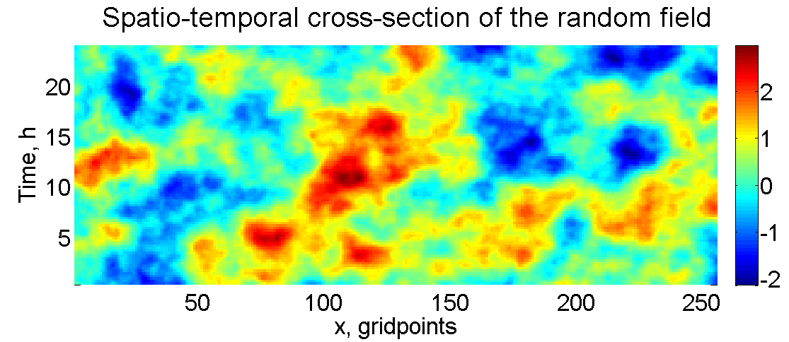
Figure 8 shows a horizontal $x$-$y$ cross-section and Fig.9 a spatio-temporal $x$-$t$ cross-section of the pseudo-random field $\xi(t,x,y)$ simulated by the SPG with the setup parameters indicated in section 6.4.3. Note that with 300 grid points in each spatial direction, only 256 contiguous grid points are shown in the Figs.8 and 9 and are intended to be used in a mapping to a physical space domain. This is done in the SPG for practical purposes in order to avoid correlations between the opposite sides of the spatial domain, which would be spurious in real-world applications.

Figure 8: Horizontal ($x$-$y$) cross-section of an SPG field.

Figure 9: Spatio-temporal ($x$-$t$) cross-section of an SPG field.

7 Discussion

7.1 Physical-space or spectral-space SPG solver?

In this study, we have investigated both the spectral-space and the physical-space approximations of the SPG spatio-temporal model. We have found that both approaches can be used to build a practical SPG scheme. We have selected the spectral-space technique. Here, we briefly compare both approaches.

Advantages of the spectral-space technique are the following.

• Simplicity of realization. If the SPG model has constant coefficients, then the complicated SPG equation decouples into a series of simple OSDEs.

• Straightforward accommodation of non-local-in-physical-space spatial operators.

Advantages of the physical-space approach are:

• The relative ease of introduction of inhomogeneous (non-stationary) and anisotropic capabilities to the SPG.

• The SPG solver can be implemented in domains with complex boundaries.

• Better suitability for an efficient implementation on massively parallel computers.

7.2 Extensions of the SPG

The proposed SPG technique can be extended in the future along the following lines.

• Development of a physical-space solver.

• Introduction of advection to the SPG model.

• Introduction of spatial inhomogeneity/anisotropy and non-stationarity.

• Introduction of non-Gaussianity. This can be done either by applying a nonlinear transform to the output SPG fields, or by introducing a non-Gaussian driving noise (as in Åberg and Podgórski, 2011, Wallin and Bolin, 2015). The former approach is simpler but the latter allows for much richer deviations from Gaussianity, including the multi-dimensional aspect.

• Going beyond additive and multiplicative perturbations for highly non-Gaussian variables like humidity, cloud fields, or precipitation.

• Simulation of several mutually correlated pseudo-random fields.

• Making the temporal order $p$ a user defined variable. As noted above, the larger $p$ the smoother the generated field.

8 Conclusions

• The proposed Stochastic Pattern Generator (SPG) produces pseudo-random spatio-temporal Gaussian fields on 2D and 3D limited area spatial domains with the tunable variance, horizontal, vertical, and temporal length scales.

• The SPG model is defined on a standardized domain in space, specifically, on the unit 2D or 3D torus. Fields on a limited-area geophysical domain in question are obtained by mapping from the standardized domain.

• The SPG is based on a linear third-order in time stochastic model driven by the white in space and time Gaussian noise.

• The spatial operator of the stochastic model is built to ensure that solutions to the SPG model, i.e. the generated pseudo-random fields, satisfy the “proportionality of scales” property: large-scale (small-scale) in space field components have large (small) temporal length scales.

• Beyond the “proportionality of scales”, the generated fields possess a number of other nice properties:

  • The spatio-temporal realizations are (almost surely) continuous.

  • With the appropriately scaled time and vertical coordinates, the spatio-temporal fields are isotropic in space-time.

  • The correlation functions in space-time belong to the Matérn class.

  • The spatial and temporal correlations have the same shapes.

• The basic SPG solver is spectral-space based.

• Two techniques to accelerate the spectral-space computations are proposed and implemented. The first technique selects the time step of the spectral-space numerical integration scheme to be dependent on the wavenumber, so that the discretization error is smaller for more energetic larger spatial scales and is allowed to be larger for less energetic smaller scales. The second technique introduces a coarse grid in spectral space. The combined speedup for spectral-space computations from both techniques is as large as 40–60 times.

• Potential applications of the SPG include ensemble prediction and ensemble data assimilation in meteorology, oceanography, hydrology, and other areas. The SPG can be used to generate spatio-temporal perturbations of the model fields (in the additive or multiplicative or other mode) and of the boundary conditions.

• An application of the SPG as a source of additive spatio-temporal model error perturbations to the meteorological COSMO model (Baldauf et al., 2011) is described in (Tsyrulnikov and Gayfulin, 2017).

Appendices

Appendix A Spatio-temporal structure of the driving 4-D noise

Here, we recall the general definition of the white noise, define the spatial spectrum of the white noise on the $d$-dimensional unit torus, and find its spatial spectral decomposition in the spatio-temporal case. Then we introduce a colored in space and white in time noise, and find it spatial spectrum. Finally, we define the time discrete complex-valued white-noise process.

A.1 White noise

By definition, see e.g. (Rozanov, 1982, section 1.1.3) or (Kuo, 2001, section 3.1.4), the (complex) standard white noise $\Omega({\bf x})$ defined on a manifold ${\mathbb{D}}$ is a generalized random field that acts on a test function $\varphi({\bf x})$ (where $x\in{\mathbb{D}}$) as follows:

$$(\Omega,\varphi):=\int\varphi({\bf x})\,\Psi({\rm d}{\bf x}),$$ (57)

where $\Psi$ is the Gaussian orthogonal stochastic measure such that for any Borel set $A$, $\Psi(A)$ is a (complex, in general) Gaussian random variable with ${\mathsf{E}\,}\Psi(A)=0$ and ${\mathsf{E}\,}|\Psi(A)|^{2}=|A|$, where $|A|$ is the Lebesgue measure of $A$.

The equivalent definitions of the standard white noise are

$${\mathsf{E}\,}|(\Omega,\varphi)|^{2}:=\int|\varphi({\bf x})|^{2}\,{\rm d}{\bf x},$$ (58)

and

$${\mathsf{E}\,}(\Omega,\varphi)\cdot\overline{(\Omega,\psi)}:=\int\varphi({\bf x})\overline{\psi({\bf x})}\,{\rm d}{\bf x},$$ (59)

where $\psi$ is another test function. Thus, we have defined of the standard white noise. By the general Gaussian white noise, we mean a multiple of the standard white noise.

A.2 Spectrum of the white noise on ${\mathbb{T}}^{\mathnormal{d}}$

The formal Fourier transform of the spatial white noise $\Omega({\bf s})$ (where ${\bf s}\in{\mathbb{T}}^{\mathnormal{d}}$),

$$\tilde{\Omega}_{\bf k}=\frac{1}{(2\pi)^{d}}\int_{{\mathbb{T}}^{\mathnormal{d}}}\Omega({\bf s})\,\rm e^{-{\mathsf{i}}({\bf k},{\bf s})}\,{\rm d}{\bf s},$$ (60)

can be rigorously justified as the action of the white noise $\Omega$ on the test function

$$\chi({\bf s}):=\frac{1}{(2\pi)^{d}}\,\rm e^{-{\mathsf{i}}({\bf k},{\bf s})}.$$ (61)

Then, the spatial spectrum of $\Omega({\bf s})$ is

$$b_{\bf k}:={\mathsf{E}\,}|\tilde{\Omega}_{\bf k}|^{2}\equiv{\mathsf{E}\,}|(\Omega,\chi)|^{2}=\int_{{\mathbb{T}}^{\mathnormal{d}}}|\chi({\bf s})|^{2}\,{\rm d}{\bf s}=\frac{1}{(2\pi)^{d}}.$$ (62)

Here, the third equality is due to Eq.(58). We stress that it is the modal spectrum that is constant for the white noise (not the variance spectrum).

A.3 Space-integrated spatio-temporal white noise on ${\mathbb{T}}^{\mathnormal{d}}\times{\mathbb{R}}$

Let us consider the spatio-temporal white noise $\Omega=\Omega(t,{\bf s})$, where $t\in{\mathbb{R}}$ is time and ${\bf s}\in{\mathbb{T}}^{\mathnormal{d}}$ the spatial coordinate vector. Take a spatial test function $c({\bf s})$ and define the temporal process $\Omega_{1}(t)$ formally as

$$\Omega_{1}(t):=\int_{{\mathbb{T}}^{\mathnormal{d}}}\Omega(t,{\bf s})c({\bf s})\,{\rm d}{\bf s},$$ (63)

so that it acts on a test function in the temporal domain, $\varphi(t)$, as

$$(\Omega_{1},\varphi):=\int_{{\mathbb{R}}}\Omega_{1}(t)\varphi(t)\,{\rm d}t=\int_{{\mathbb{R}}}\int_{{\mathbb{T}}^{\mathnormal{d}}}\Omega(t,{\bf s})c({\bf s})\varphi(t)\,{\rm d}{\bf s}\,{\rm d}t.$$ (64)

Here, we note that the latter double integral is nothing other than the result of action of the original white noise $\Omega(t,{\bf s})$ on the spatio-temporal test function $c({\bf s})\cdot\varphi(t)$. This enables us to mathematically rigorously define $\Omega_{1}(t)$ as the generalized random process that, with the fixed $c({\bf s})$, acts on the test function $\varphi(t)$ as follows:

$$(\Omega_{1}(t),\varphi(t)):=(\Omega(t,{\bf s}),\,c({\bf s})\varphi(t)).$$ (65)

Now, using the definition Eq.(58) of the white noise $\Omega(t,{\bf s})$, we have

$${\mathsf{E}\,}|(\Omega(t,{\bf s}),\,c({\bf s})\varphi(t))|^{2}=\int_{{\mathbb{T}}^{\mathnormal{d}}}\int_{{\mathbb{R}}}|c({\bf s})|^{2}|\varphi(t)|^{2}\,{\rm d}{\bf s}\,{\rm d}t=\int_{{\mathbb{T}}^{\mathnormal{d}}}|c({\bf s})|^{2}\,{\rm d}{\bf s}\int_{{\mathbb{R}}}|\varphi(t)|^{2}\,{\rm d}t.$$ (66)

Since we have fixed $c({\bf s})$, we observe that

$$\sigma^{2}:=\int|c({\bf s})|^{2}\,{\rm d}{\bf s}$$ (67)

is a constant such that

$${\mathsf{E}\,}|(\Omega_{1}(t),\varphi(t))|^{2}=\sigma^{2}\int_{{\mathbb{R}}}|\varphi(t)|^{2}\,{\rm d}t.$$ (68)

Comparing this equation with one of the definitions of the standard white noise, Eq.(58), we recognize $\Omega_{1}(t)$ as a general Gaussian white noise in time, i.e. the standard temporal white noise multiplied by $\sigma$. We call $\sigma$ the intensity of the white noise.

A.4 Spatial spectrum of a spatio-temporal white noise

Now, we are in a position to derive the spatial spectrum of the standard spatio-temporal white noise $\Omega(t,{\bf s})$. In the formal Fourier decomposition

$$\Omega(t,{\bf s})=\sum_{\bf k}\tilde{\Omega}_{\bf k}(t)\,\rm e^{{\mathsf{i}}({\bf k},{\bf s})},$$ (69)

the elementary temporal processes $\tilde{\Omega}_{\bf k}(t)$ can be shown to be white noises in time. Indeed, again formally, we have

$$\tilde{\Omega}_{\bf k}(t)=\frac{1}{(2\pi)^{d}}\int_{{\mathbb{T}}^{\mathnormal{d}}}\Omega(t,{\bf s})\,\rm e^{-{\mathsf{i}}({\bf k},{\bf s})}\,{\rm d}{\bf s}.$$ (70)

Here, we recognize an expression of the kind given by Eq.(63) with $c({\bf s}):=\rm e^{-{\mathsf{i}}({\bf k},{\bf s})}/(2\pi)^{d}$. Therefore, from Eq.(68), $\tilde{\Omega}_{\bf k}(t)$ is a temporal white noise with the intensity $\sigma_{\bf k}^{\Omega}$ squared equal to

$$(\sigma_{\bf k}^{\Omega})^{2}=\int|c({\bf s})|^{2}\,{\rm d}{\bf s}=\frac{1}{(2\pi)^{2d}}\int_{{\mathbb{T}}^{\mathnormal{d}}}|\rm e^{-{\mathsf{i}}({\bf k},{\bf s})}|^{2}\,{\rm d}{\bf s}=\frac{1}{(2\pi)^{d}}.$$ (71)

In addition, using Eq.(59), it is easy to show that $\tilde{\Omega}_{\bf k}(t)$ and $\tilde{\Omega}_{\bf k^{\prime}}(t)$ are mutually orthogonal for ${\bf k}\neq{\bf k}^{\prime}$.

To summarize, $\tilde{\Omega}_{\bf k}(t)$ are mutually orthogonal white-in-time noises, all with equal intensities $\sigma_{\bf k}^{\Omega}=(2\pi)^{-d/2}$:

$$\tilde{\Omega}_{\bf k}(t)=\frac{1}{(2\pi)^{d/2}}\,\Omega_{\bf k}(t),$$ (72)

where $\Omega_{\bf k}(t)$ are the standard white noises.

Note that if we consider the non-unit torus ${\mathbb{T}}^{\mathnormal{d}}(R)={\mathbb{S}}^{1}(R)\times\dots\times{\mathbb{S}}^{1}(R)$ ($d$ times), where $R$ is the radius of each circle, then, obviously, in Eqs.(70)–(72), $2\pi$ is to be replaced by $2\pi R$.

A.5 Spectral decomposition of a white in time and colored in space noise

In order to introduce a white in time and colored in space noise, let us convolve the spatio-temporal white noise $\Omega(t,{\bf s})$ with a smoothing kernel in space $u({\bf s})$, getting

$$\alpha(t,{\bf s}):=\int_{{\mathbb{T}}^{\mathnormal{d}}}u({\bf s-r})\,\Omega(t,{\bf r})\,{\rm d}{\bf r}.$$ (73)

In this equation, the stochastic integral is defined, for any $t$ and ${\bf s}$, following Eq.(65) with $c({\bf r}):=u({\bf s-r})$. Fourier transforming $u({\bf s})$,

$$u({\bf s})=\sum_{\bf k}\tilde{u}_{\bf k}\,\rm e^{{\mathsf{i}}({\bf k},{\bf s})},$$ (74)

and, in space, $\alpha(t,{\bf s})$,

$$\alpha(t,{\bf s})=\sum_{\bf k}\tilde{\alpha}_{\bf k}(t)\,\rm e^{{\mathsf{i}}({\bf k},{\bf s})},$$ (75)

we easily obtain that the elementary spectral processes $\tilde{\alpha}_{\bf k}(t)$ are independent white noises in time with the intensities squared

$$\sigma_{\bf k}^{2}=(2\pi)^{d}|\tilde{u}_{\bf k}|^{2},$$ (76)

so that the stochastic differential $\tilde{\alpha}_{\bf k}(t){\rm d}t$ is

$$\tilde{\alpha}_{\bf k}(t)\,{\rm d}t=\sigma_{\bf k}\,{\rm d}W_{\bf k}(t).$$ (77)

Equivalently,

$$\tilde{\alpha}_{\bf k}(t)=\sigma_{\bf k}\,\Omega_{\bf k}(t).$$ (78)

A.6 Discretization of the spectral processes $\tilde{\alpha}_{\bf k}(t)$ in time

Being white noises, $\tilde{\alpha}_{\bf k}(t)$ have infinite variances. They become ordinary random processes if, e.g., we discretize them in time. With the time step $\Delta t$, we define the discretized process $\hat{\alpha}_{\bf k}(t_{j})$ at the time instance $t_{j}$ by replacing, in Eq.(77), ${\rm d}t$ with $\Delta t$ and ${\rm d}W_{\bf k}$ with $\Delta W_{\bf k}$:

$$\hat{\alpha}_{\bf k}(t_{j})\,\Delta t:=\sigma_{\bf k}\,\Delta W_{\bf k}(t).$$ (79)

As ${\mathsf{E}\,}|\Delta W_{\bf k}(t)|^{2}=\Delta t$, we obtain

$$\hat{\alpha}_{\bf k}(t_{j})=\frac{\sigma_{\bf k}}{\sqrt{\Delta t}}\cdot\zeta_{{\bf k}j},$$ (80)

where $\zeta_{{\bf k}j}$ are independent complex standard Gaussian random variables $CN(0,1)$. The latter is defined as a complex random variable whose real and imaginary parts are mutually uncorrelated zero-mean random variables with variances equal to $1/2$. $CN(0,1)$ is sometimes referred to as the circularly symmetric complex Gaussian (normal) random variable (e.g. Tse and Viswanath, 2005).

Equation (80) shows that the spatial spectrum of the time discrete driving noise is $\sigma_{\bf k}^{2}/\Delta t$.

Appendix B Physical-space approximation of the operator $\sqrt{1-\lambda^{2}\Delta}$

As we have discussed in section 4.5, the fractional power (square root) of the negated and shifted Laplacian operator, ${\cal L}:=\sqrt{1-\lambda^{2}\Delta}$, is defined as the pseudo-differential operator with the symbol $\tilde{l}({\bf k}):=\sqrt{1+\lambda^{2}{\bf k}^{2}}$. In the literature, one can find approaches to discretization of fractional powers of elliptic operators, e.g. Simpson et al. (2012) used finite elements in the spatial context.

Here, we propose a simple technique to build a spatial discretization scheme that approximates the operator $\sqrt{1-\lambda^{2}\Delta}$ in the sense that the symbol of the approximating operator is close to $\sqrt{1+\lambda^{2}{\bf k}^{2}}$.

To this end, we do the following.

1. Perform the backward Fourier transform of the symbol $\tilde{l}({\bf k})$, getting the function $l({\bf s})$. As multiplication in Fourier space by $\tilde{l}({\bf k})$ is equivalent to convolution in physical space with $l({\bf s})$, we obtain that for any test function $\varphi({\bf s})$,

   $$({\cal L}\varphi)({\bf s})=\int_{{\mathbb{T}}^{3}}l({\bf s-r})\,\varphi({\bf r})\,{\rm d}{\bf r}.$$ (81)

   The crucial moment here is that the kernel function $l({\bf s})$ appears to be oscillating while rapidly decreasing in modulus as $|{\bf s}|$ increases (see below). This enables its efficient approximation with a compact-support (truncated) function.

2. With the discretization on the grid with $n$ points in each of the $d$ dimensions on the torus ${\mathbb{T}}^{\mathnormal{d}}$, the kernel function $l({\bf s})$ is represented by the set of its grid-point values $l({\bf s}_{\bf i})$, where ${\bf s}=(s_{1},\dots,s_{d})$, ${\bf i}=(i_{1},\dots,i_{d})$, and ${\bf s}_{\bf i}=(s_{1}({i_{1}}),\dots,s_{d}({i_{d}}))$. If $l({\bf s})$ appears to be rapidly decreasing away from ${\bf s=0}$, we truncate the $l({\bf s}_{\bf i})$ function by limiting its support near the origin, thus getting the function $l_{\rm trunc}({\bf s}_{\bf i})$. E.g. in 3D, the support of $l_{\rm trunc}({\bf s}_{\bf i})$ consists of the grid points ${\bf i}=(i_{1},i_{2},i_{3})$ that simultaneously satisfy the following constraints: $|i_{1}|\leq J$, $|i_{2}|\leq J$, and $|i_{3}|\leq J$, where $J$ is the spatial order of the scheme. Below, we present results with $J=1$ (3 grid points in the support of the truncated kernel function in each dimension) and $J=3$ (7 grid points in the support in each dimension).

3. Fourier transform $l_{\rm trunc}({\bf s})$ back to the spectral space, getting the approximated symbol $\tilde{l}_{\rm trunc}({\bf k})$.

4. Compare $\tilde{l}({\bf k})$ with $\tilde{l}_{\rm trunc}({\bf k})$ and conclude whether a parsimonious (that is, with a very small $J$) approximation is viable.

Now, we present the results. We found that for $d=1$, $d=2$, and $d=3$, the goodness of fit was similar, so we examine the 3D case below.

We selected the grid of $n=2\cdot n_{\rm max}=256$ points in each of the three dimensions. We specified the spatial non-dimensional length scale $\lambda$ to be much greater than the mesh size $h=2\pi/n$ and much less than the domain’s extents, $2\pi$. Specifically, we chose $\lambda=1/n_{1}$, where $n_{1}:=\sqrt{n_{\rm max}}$. (The results were not much sensitive to changes in $n_{1}$ within the whole wavenumber range on the grid.)

Figure 10 displays the resulting kernel function $l({s})$ for positive $s$ (note that $l({s})$ is an even function of the scalar distance $s$). One can see the remarkably fast decay of $|l({s})|$ with the growing $s$. Consequently, a stencil with just a few points in each dimension can be expected to work well.

Figure 10: The kernel function

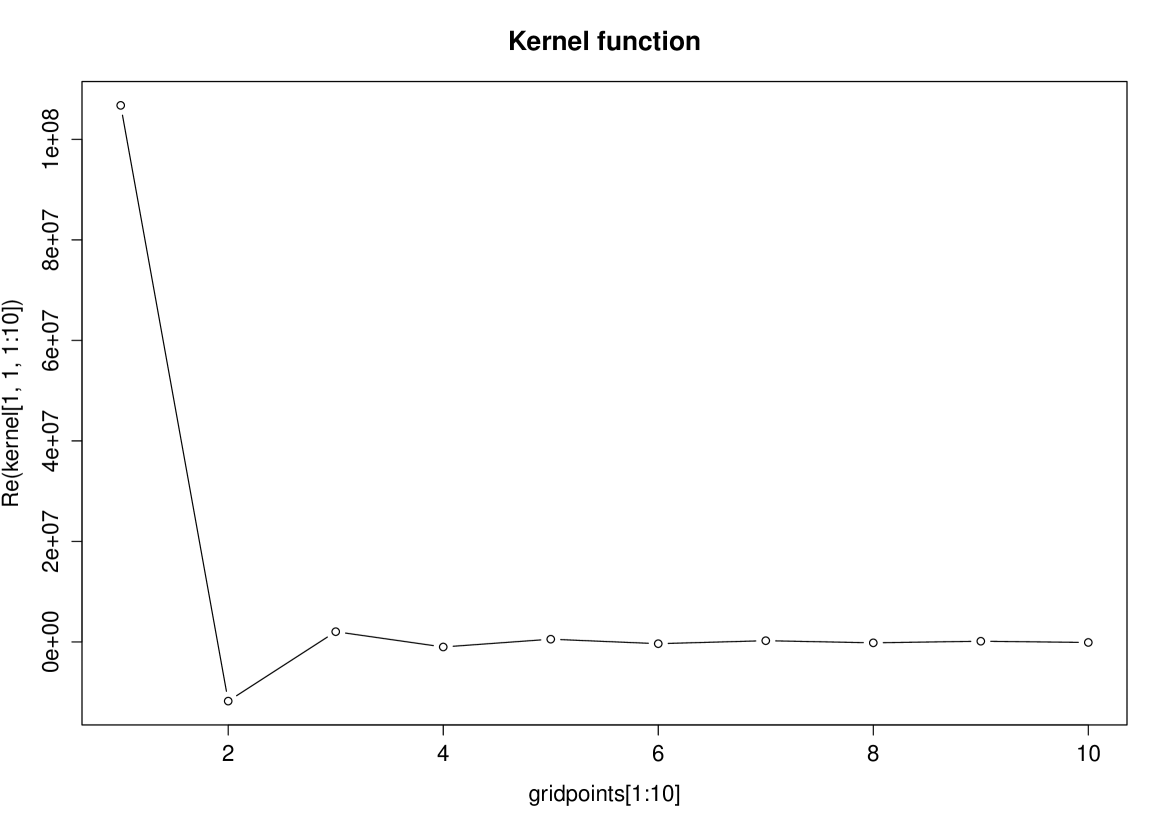
Figure 11 shows the exact and approximated symbols for the stencil that contains 3 grid points in each dimension (the left panel) and the stencil that contains 7 grid points in each dimension (the right panel). (The 5-point scheme worked not much better than the 3-point one and so its performance is not shown.)

Figure 11: Goodness of fit of the symbol $\tilde{l}({\bf k})$ (solid curve) by $\tilde{l}_{\rm trunc}({\bf k})$ (circles). Left: the 3-point stencil in each dimension. Right: the 7-point stencil

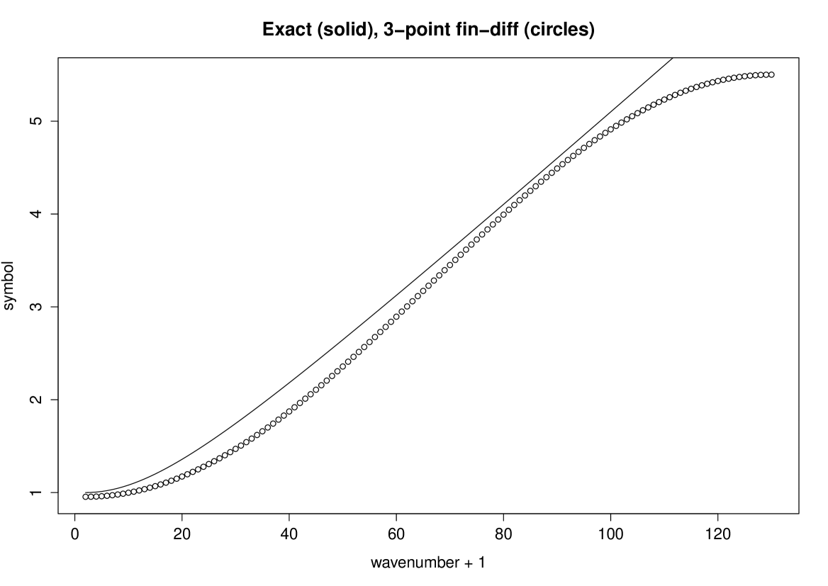
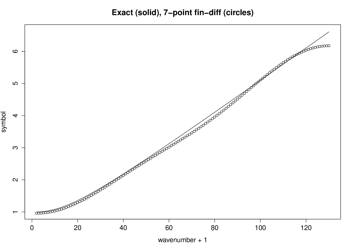
From Fig.11, one can see that the 3-point scheme’s performance is rather mediocre, whereas the 7-point scheme works very well (in terms of the reproduction of the operator’s symbol).

Finally, we verified that the symbol $\tilde{l}_{\rm trunc}({\bf k})$ of the discrete operator for $J=3,5,7$ was everywhere positive, which guarantees that the operator is positive definite and so the discretized SPG model should be stable.

To summarize, the operator $\sqrt{1-\lambda^{2}\Delta}$ can be approximated with parsimonious physical-space discretization schemes. For simulation of uncertainty in meteorology, where precise error statistics is not available, the simplest 3-point (in each direction) scheme seems most appropriate and computationally attractive. For more demanding applications, the 7-point scheme can be more appropriate.

Appendix C Stationary statistics of a higher-order OSDE

We examine the OSDE Eq.(30) in its generic form:

$$\left(\frac{{\rm d}}{{\rm d}t}+a\right)^{p}\eta(t)=\sigma\Omega(t),$$ (82)

where $\eta(t)$ is the random process in question, $\sigma$ and $a$ are the positive numbers, $p$ is the positive integer, and $\Omega(t)$ is the standard white noise, see e.g. Rozanov (1982, section 1.1.3) or Kuo (2001, section 3.1.4) and also Appendix A.1.

The goal here is to find the variance and the correlation function of $\eta(t)$ in the stationary regime. The technique is to reduce the $p$-th order OSDE to a system of first-order OSDEs.

To simplify the exposition, we consider the third-order OSDE ($p=3$) and rewrite Eq.(82) as

$$\left(\frac{{\rm d}}{{\rm d}t}+a\right)\,\,\,\,\left\{\left(\frac{{\rm d}}{{\rm d}t}+a\right)\,\,\left[\left(\frac{{\rm d}}{{\rm d}t}+a\right)\eta(t)\right]\right\}=\sigma\Omega(t).$$ (83)

Here, by $\eta_{1}$ we denote the term in brackets,

$$\left(\frac{{\rm d}}{{\rm d}t}+a\right)\eta=\eta_{1}$$ (84)

and by $\eta_{2}$ the term in braces,

$$\left(\frac{{\rm d}}{{\rm d}t}+a\right)\eta_{1}=\eta_{2},$$ (85)

so that Eq.(83) implies that

$$\left(\frac{{\rm d}}{{\rm d}t}+a\right)\eta_{2}=\sigma\Omega.$$ (86)

In Eqs.(84)–(86), the last equation is the familiar first-order OSDE forced by the white noise, whereas the other equations are not forced by the white noise. Generalizing the above construction, Eqs.(83)–(86), to the arbitrary $p>0$, we form the following first-order vector-matrix OSDE (a system of first-order OSDEs):

$${\rm d}\boldsymbol{\eta}+{\bf A}\boldsymbol{\eta}{\rm d}t=\boldsymbol{\Sigma}\boldsymbol{\Omega}{\rm d}t,$$ (87)

where $\boldsymbol{\eta}=(\eta,\eta_{1},\dots,\eta_{p-2},\eta_{p-1})$, $\boldsymbol{\Omega}=(0,0,\dots,0,\Omega)$ , and the design of the matrices ${\bf A}$ and $\boldsymbol{\Sigma}$ is obvious (not shown).

With Eq.(87) in hand, we derive a differential equation for the covariance matrix ${\bf P}={\mathsf{E}\,}\boldsymbol{\eta}\boldsymbol{\eta}^{*}$, where ^∗ denotes transpose complex conjugate (e.g. Jazwinski, 1970, example 4.16). First, we compute the increment of ${\bf P}$:

$$\Delta{\bf P}={\mathsf{E}\,}(\boldsymbol{\eta}+{\rm d}\boldsymbol{\eta})(\boldsymbol{\eta}+{\rm d}\boldsymbol{\eta})^{*}-{\mathsf{E}\,}\boldsymbol{\eta}\boldsymbol{\eta}^{*}={\mathsf{E}\,}\boldsymbol{\eta}{\rm d}\boldsymbol{\eta}^{*}+{\mathsf{E}\,}{\rm d}\boldsymbol{\eta}\boldsymbol{\eta}^{*}+{\mathsf{E}\,}{\rm d}\boldsymbol{\eta}{\rm d}\boldsymbol{\eta}^{*}.$$ (88)

Then, using Eq.(87) and the fact that ${\mathsf{E}\,}|\Omega{\rm d}t|^{2}={\mathsf{E}\,}|{\rm d}W|^{2}={\rm d}t$, we obtain the differential of ${\bf P}$ from Eq.(88):

$${\rm d}{\bf P}=-{\bf A}{\bf P}{\rm d}t-{\bf P}{\bf A}^{*}{\rm d}t+\boldsymbol{\Sigma}\boldsymbol{\Sigma}^{*}{\rm d}t.$$ (89)

In the stationary regime ${\rm d}{\bf P}=0$, so the equation for the stationary covariance matrix is

$${\bf A}{\bf P}+{\bf P}{\bf A}^{*}=\boldsymbol{\Sigma}\boldsymbol{\Sigma}^{*}.$$ (90)

This a system of linear algebraic equations for the unknown entries of the matrix ${\bf P}$. Because both ${\bf P}$ and $\boldsymbol{\Sigma}\boldsymbol{\Sigma}^{*}$ are self-adjoint matrices, the number of unknowns, $p(p+1)/2$, is equal to the number of independent equations. We analytically solve this system of equations and look at the first diagonal entry of the solution ${\bf P}$, which represents the required ${\mathsf{Var}}\,\eta$ (because the random field in question $\eta$ is defined above to be the first entry of the vector $\boldsymbol{\eta}$). Dropping tedious derivations, we present in Table 3 (the second row) the formulas for the temporal orders $p=1$, $p=2$, $p=3$, and for the general $p$.

Finally, we derive the temporal correlation function for the $p$th-order OSDE. To this end, we multiply Eq.(82) by $\eta(s)$ with $s<t$ and take expectation. Since $a$ is non-stochastic, we may interchange the expectation and the differential operator $\left(\frac{{\rm d}}{{\rm d}t}+a\right)^{p}$, getting the $p$th-order ordinary differential equation for the temporal covariance function, whose solutions for different $p$ are presented in row 3 of Table 3.

Table 3: Variances ${\mathsf{Var}}\,\eta$ and correlation functions $C_{\eta}(t)$ of the stationary solution to Eq.(82) for different temporal orders $p$.

$p$	$1$	$2$	$3$	Arbitrary $p$
${\mathsf{Var}}\,\eta$	$\frac{\sigma^{2}}{2a}$	$\frac{\sigma^{2}}{4a^{3}}$	$\frac{3\sigma^{2}}{16a^{5}}$	$\frac{\sigma^{2}}{a^{2p-1}}$
$C_{\eta}(t)$	$\rm e^{\mathnormal{-a|t|}}$	$(1+a|t|)\,\rm e^{\mathnormal{-a|t|}}$	$(1+a|t|+\frac{a^{2}t^{2}}{3})\,\rm e^{\mathnormal{-a|t|}}$	$R_{p-1}(a|t|)\cdot\rm e^{\mathnormal{-a|t|}}$

Note that $R_{p-1}(.)$ in the last row of the table stands for the polynomial of order $p-1$.

Appendix D Smoothness of sample paths of the spatial Matérn random field for different $\nu$

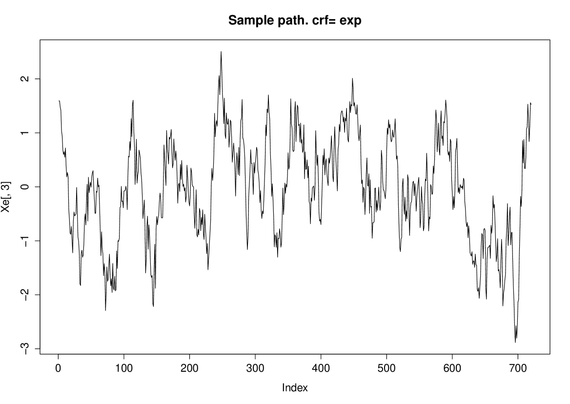
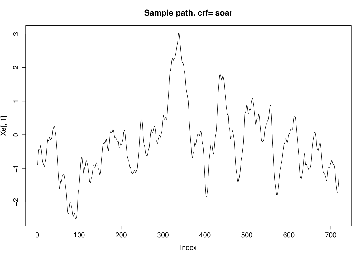
Here, we show how sample paths (realizations) of the Matérn random field with the smoothness parameter $\nu$ look. Specifically, in Fig.12, we present three plots with 1D cross-sections of randomly chosen realizations of the Matérn random field for the following three values of $\nu$: 1/2, 3/2, and 5/2. The spatial length scale parameter $\lambda$ is selected in each of the three cases in such a way that the spatial correlation function intersects the 0.7 level at approximately the same distance (we denote this distance by $L_{0.7}$): $L_{0.7}=500$ km. Note that, as in section 5.6, we assume, for convenience, that the extent of the spatial domain in each coordinate direction is 3000 km (rather than $2\pi$). For comparison, we also display a realization with $L_{0.7}=1500$ km for $\nu=1/2$ (the bottom panel of Fig.12).

Figure 12: Sample paths for various $\nu$ and $L_{0.7}$. From the top to the bottom:
($\nu=\frac{1}{2}$, $L_{0.7}=500$), ($\nu=\frac{3}{2}$, $L_{0.7}=500$), ($\nu=\frac{5}{2}$, $L_{0.7}=500$), ($\nu=\frac{1}{2}$, $L_{0.7}=1500$)

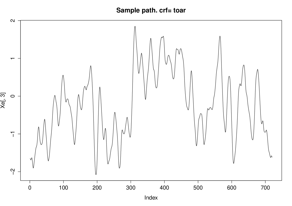
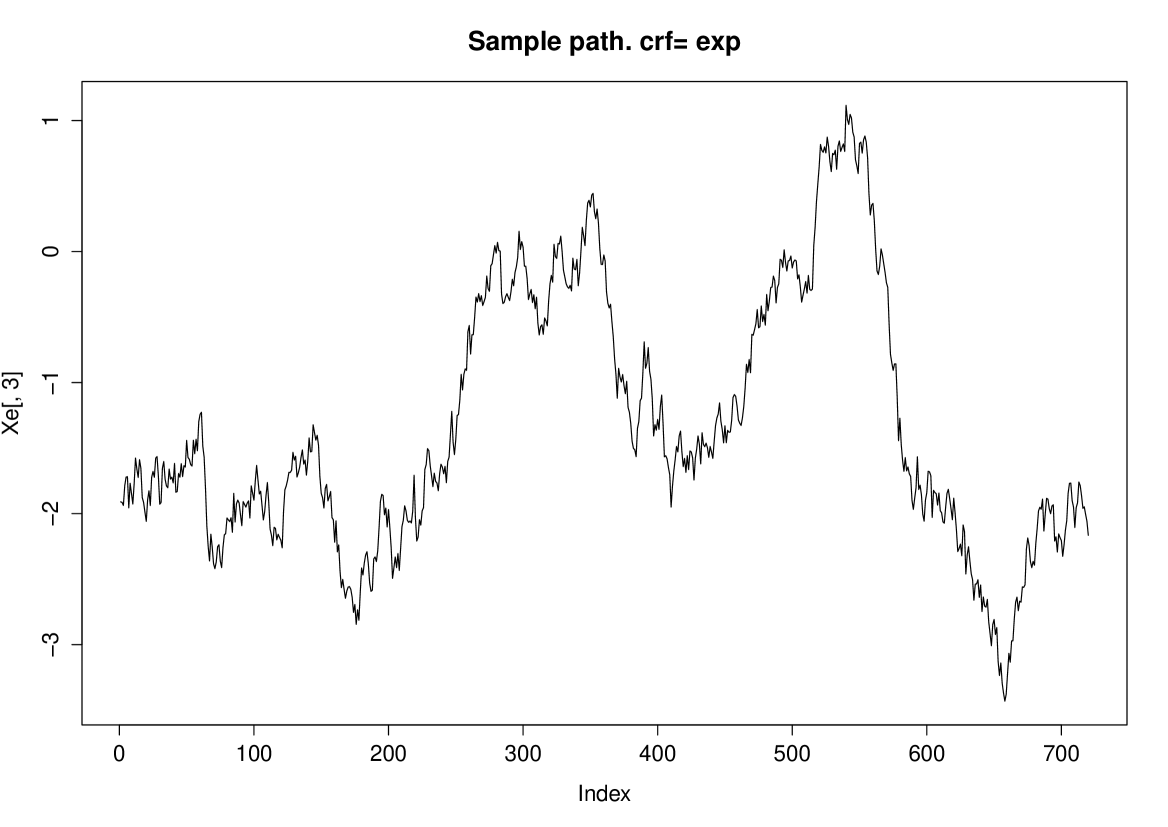
One can see that, indeed, the larger $\nu$, the smoother the realizations—in the sense that they have less small-scale “noise”. By contrast, increasing the length scale $\lambda$ (compare the top and bottom panels of Fig.12) makes the large-scale pattern smoother but does not remove the smallest scales. So, the large-scale behavior is determined by the length scale $\lambda$, whereas the degree of small-scale smoothness/roughness depends predominantly on the smoothness parameter $\nu$.

Appendix E Stationary statistics of a time discrete higher-order OSDE

Here, to simplify the exposition, we first examine the simplest first-order (i.e. with $p=1$) OSDE and then give the results for the third-order OSDE used in the current version of the SPG.

E.1 First-order numerical scheme

Discretization of the Langevin Eq.(14) by an implicit scheme yields

$$\eta_{i}-\eta_{i-1}+a\eta_{i}\,\Delta t=\sigma\Delta W_{i},$$ (91)

so that

$$\eta_{i}=\frac{\eta_{i-1}+\sigma\Delta W_{i}}{1+a\Delta t}.$$ (92)

In the stationary regime, ${\mathsf{Var}}\,\eta_{i}={\mathsf{Var}}\,\eta_{i-1}$, whence, bearing in mind that ${\mathsf{Var}}\,\Delta W_{i}=\Delta t$ and $\Delta W_{i}$ is independent on the values of $\eta$ for all time moments up to and including the moment $i-1$, we apply the variance operator to both sides of Eq.(92) and obtain the stationary variance

$$V(\Delta t):=\lim_{i\to\infty}{\mathsf{Var}}\,\eta_{i}=\frac{\sigma^{2}}{2a+(g\Delta t)^{2}}.$$ (93)

Note that, as $\Delta t\to 0$, $V(\Delta t)$ tends to the continuous-time variance $\frac{\sigma^{2}}{2a}$, see Eq.(15).

E.2 Third-order numerical scheme

Consider the continuous-time OSDE, Eq.(82), with $p=3$. The implicit scheme Eq.(53) we use to numerically solve it is reproduced here as

$$\eta_{i}=\frac{1}{\varkappa^{3}}\left[3\varkappa^{2}\eta_{i-1}-3\varkappa\eta_{i-2}+\eta_{i-3}+\sigma(\Delta t)^{2}\,\Delta W_{i}\right],$$ (94)

where $\varkappa:=1+a\Delta t$. Here, the goal is to find the stationary variance $V:=\lim_{i\to\infty}{\mathsf{Var}}\,\eta_{i}$ along with lag-1 and lag-2 stationary covariances, $c_{1}:=\lim_{i\to\infty}{\mathsf{E}\,}\eta_{i}\eta_{i-1}$ and $c_{2}:=\lim_{i\to\infty}{\mathsf{E}\,}\eta_{i}\eta_{i-2}$, respectively. To reach this goal, we build three linear algebraic equations for the three unknowns, $V$, $c_{1}$, and $c_{2}$. The first equation is obtained by applying the variance operator to both sides of Eq.(94). The second and third equations are obtained by multiplying Eq.(94) by $\eta_{i-1}$ and $\eta_{i-2}$, respectively, and applying the expectation operator to both sides of the resulting equations. Omitting the derivations, we write down the results:

$$V=\frac{\varkappa^{4}+4\varkappa^{2}+1}{(\varkappa^{2}-1)^{5}}\,(\Delta t)^{5}\sigma^{2}.$$ (95)

$$c_{1}=\frac{3\varkappa(\varkappa^{2}+1)}{(\varkappa^{2}-1)^{5}}\,(\Delta t)^{5}\sigma^{2},\qquad c_{2}=\frac{6\varkappa^{2}}{(\varkappa^{2}-1)^{5}}\,(\Delta t)^{5}\sigma^{2}.$$ (96)

As in the first-order case, one can see that as $\Delta t\to 0$, $V$ tends to the continuous-time variance $\frac{3}{16}\frac{\sigma^{2}}{a^{5}}$, see Table 3.

References

- Åberg and Podgórski (2011) S. Åberg and K. Podgórski. A class of non-Gaussian second order random fields. Extremes, 14(2):187–222, 2011.
- Adler (1981) R. J. Adler. The geometry of random fields. Wiley, 1981.
- Arnold (1974) L. Arnold. Stochastic differential equations. Wiley, 1974.
- Baldauf et al. (2011) M. Baldauf, A. Seifert, J. Förstner, D. Majewski, M. Raschendorfer, and T. Reinhardt. Operational convective-scale numerical weather prediction with the COSMO model: description and sensitivities. Mon. Wea. Rev., 139(12):3887–3905, 2011.
- Bengtsson et al. (2013) L. Bengtsson, M. Steinheimer, P. Bechtold, and J.-F. Geleyn. A stochastic parametrization for deep convection using cellular automata. Quart. J. Roy. Meteor. Soc., 139(675):1533–1543, 2013.
- Berner and Coauthors (2017) J. Berner and Coauthors. Stochastic parameterization: Towards a new view of weather and climate models. Bull. Amer. Meteor. Soc., 98(3):565–587, 2017.
- Berner et al. (2009) J. Berner, G. Shutts, M. Leutbecher, and T. Palmer. A spectral stochastic kinetic energy backscatter scheme and its impact on flow-dependent predictability in the ECMWF ensemble prediction system. J. Atmos. Sci., 66(3):603–626, 2009.
- Berner et al. (2011) J. Berner, S.-Y. Ha, J. Hacker, A. Fournier, and C. Snyder. Model uncertainty in a mesoscale ensemble prediction system: Stochastic versus multiphysics representations. Mon. Wea. Rev., 139(6):1972–1995, 2011.
- Bouttier et al. (2012) F. Bouttier, B. Vié, O. Nuissier, and L. Raynaud. Impact of stochastic physics in a convection-permitting ensemble. Mon. Wea. Rev., 140(11):3706–3721, 2012.
- Buizza et al. (1999) R. Buizza, M. Miller, and T. Palmer. Stochastic representation of model uncertainties in the ECMWF ensemble prediction system. Quart. J. Roy. Meteor. Soc., 125(560):2887–2908, 1999.
- Charron et al. (2010) M. Charron, G. Pellerin, L. Spacek, P. Houtekamer, N. Gagnon, H. L. Mitchell, and L. Michelin. Toward random sampling of model error in the Canadian ensemble prediction system. Mon. Wea. Rev., 138(5):1877–1901, 2010.
- Christensen et al. (2015) H. Christensen, I. Moroz, and T. Palmer. Stochastic and perturbed parameter representations of model uncertainty in convection parameterization. J. Atmos. Sci., 72(6):2525–2544, 2015.
- Cressie and Huang (1999) N. Cressie and H.-C. Huang. Classes of nonseparable, spatio-temporal stationary covariance functions. J. Amer. Statist. Assoc., 94(448):1330–1339, 1999.
- Epstein (1969) E. S. Epstein. Stochastic dynamic prediction. Tellus, 21(6):739–759, 1969.
- Gneiting et al. (2006) T. Gneiting, M. G. Genton, and P. Guttorp. Geostatistical space-time models, stationarity, separability, and full symmetry. Monographs Statist. Appl. Probab., 107:151, 2006.
- Guttorp and Gneiting (2006) P. Guttorp and T. Gneiting. Studies in the history of probability and statistics XLIX. On the Matern correlation family. Biometrika, 93(4):989–995, 2006.
- Jazwinski (1970) A. Jazwinski. Stochastic processes and filtering theory. Academic Press, 1970.
- Kuo (2001) H.-H. Kuo. White noise theory. In “Handbook of stochastic analysis and applications” Kannan D. and Lakshmikantham V. (Eds.), pages 107–158, 2001.
- Lindgren et al. (2011) F. Lindgren, H. Rue, and J. Lindström. An explicit link between Gaussian fields and Gaussian Markov random fields: the stochastic partial differential equation approach. J. Roy. Statist. Soc. B, 73(4):423–498, 2011.
- Meunier and Zhao (2009) N. Meunier and J. Zhao. Observations of photospheric dynamics and magnetic fields: from large-scale to small-scale flows. Space Sci. Rev., 144(1-4):127–149, 2009.
- Monin and Yaglom (2013) A. Monin and A. M. Yaglom. Statistical fluid mechanics, Volume II: Mechanics of turbulence. Courier Corp., 2013.
- Ollinaho et al. (2017) P. Ollinaho, S.-J. Lock, M. Leutbecher, P. Bechtold, A. Beljaars, A. Bozzo, R. M. Forbes, T. Haiden, R. J. Hogan, and I. Sandu. Towards process-level representation of model uncertainties: Stochastically perturbed parametrisations in the ECMWF ensemble. Quart. J. Roy. Meteor. Soc., 143(702):408–422, 2017.
- Orrell et al. (2001) D. Orrell, L. Smith, J. Barkmeijer, and T. Palmer. Model error in weather forecasting. Nonlin. Proc. Geophys., 8(6):357–371, 2001.
- Palmer et al. (2009) T. Palmer, R. Buizza, F. Doblas-Reyes, T. Jung, M. Leutbecher, G. Shutts, M. Steinheimer, and A. Weisheimer. Stochastic parametrization and model uncertainty. ECMWF Tech. Memo. n. 598, ECMWF, Shinfield Park, 42 pp., 2009.
- Pitcher (1977) E. J. Pitcher. Application of stochastic dynamic prediction to real data. J. Atmos. Sci., 34(1):3–21, 1977.
- Rozanov (1982) Y. A. Rozanov. Markov random fields. Springer, 1982.
- Shubin (1987) M. A. Shubin. Pseudodifferential operators and spectral theory. Springer, 1987.
- Shutts (2005) G. Shutts. A kinetic energy backscatter algorithm for use in ensemble prediction systems. Quart. J. Roy. Meteor. Soc., 131(612):3079–3102, 2005.
- Simpson et al. (2012) D. Simpson, F. Lindgren, and H. Rue. Think continuous: Markovian Gaussian models in spatial statistics. Spatial Statist., 1:16–29, 2012.
- Stein (1999) M. L. Stein. Interpolation of spatial data: some theory for kriging. Springer, New York, 1999.
- Stein (2005) M. L. Stein. Space–time covariance functions. J. Amer. Statist. Assoc., 100(469):310–321, 2005.
- Tatarsky (1969) B. Tatarsky. The use of dynamic equations for a probabilistic forecasting of the pressure fields. Izv. Akad. Nauk SSSR, FAO, 5:293–297, 1969.
- Theiler et al. (1992) J. Theiler, S. Eubank, A. Longtin, B. Galdrikian, and J. D. Farmer. Testing for nonlinearity in time series: the method of surrogate data. Physica D, 58(1-4):77–94, 1992.
- Tse and Viswanath (2005) D. Tse and P. Viswanath. Fundamentals of wireless communication. Cambridge University Press, 2005.
- Tsyroulnikov (2001) M. D. Tsyroulnikov. Proportionality of scales: An isotropy-like property of geophysical fields. Quart. J. Roy. Meteor. Soc., 127(578):2741–2760, 2001.
- Tsyrulnikov and Gayfulin (2017) M. Tsyrulnikov and D. Gayfulin. A limited-area spatio-temporal stochastic pattern generator for simulation of uncertainties in ensemble applications. Meteorol. Zeitschrift, 26(5):549–566, 2017.
- Tsyrulnikov and Gorin (2013) M. Tsyrulnikov and V. Gorin. Are atmospheric-model tendency errors perceivable from routine observations? COSMO Newsletter No. 13, pages 3–18, 2013.
- Tsyrulnikov (2005) M. D. Tsyrulnikov. Stochastic modelling of model errors: A simulation study. Quart. J. Roy. Meteor. Soc., 131(613):3345–3371, 2005.
- Wallin and Bolin (2015) J. Wallin and D. Bolin. Geostatistical modelling using non-Gaussian Matérn fields. Scand. J. Statist., 42(3):872–890, 2015.
- Yaglom (1987) A. M. Yaglom. Correlation theory of stationary and related random functions, Volume 1: Basic results. Springer-Verlag, 1987.