A determination of $m_{c}(m_{c})$ from HERA data using a matched heavy-flavor scheme

Abstract

The charm quark mass is one of the fundamental parameters of the Standard Model Lagrangian. In this work we present a determination of the $\overline{\rm MS}$ charm mass from a fit to the inclusive and charm HERA deep-inelastic structure function data. The analysis is performed within the xFitter framework, with structure functions computed in the FONLL general-mass scheme as implemented in APFEL. In the case of the FONLL-C scheme, we obtain $m_{c}(m_{c})=1.335\pm 0.043\mbox{(exp)}^{+0.019}_{-0.000}\mbox{(param)}^{+0.011}_{-0.008}\mbox{(mod)}^{+0.033}_{-0.008}\mbox{(th)}\mbox{ GeV.}$ We also perform an analogous determination in the fixed-flavor-number scheme at next-to-leading order, finding $m_{c}(m_{c})=1.318\pm 0.054\mbox{(exp)}^{+0.011}_{-0.010}\mbox{(param)}^{+0.015}_{-0.019}\mbox{(mod)}^{+0.045}_{-0.004}\mbox{(th)}\mbox{ GeV,}$ compatible with the FONLL-C value. Our results are consistent with previous determinations from DIS data as well as with the PDG world average.

1 Introduction

The masses of the heavy quarks, charm, bottom and top, are fundamental parameters of the Standard Model Moch:2014tta . A precise determination of their values is of utmost importance; as an example, the fate of the electroweak vacuum depends crucially on the exact value of $m_{t}$ Degrassi:2012ry . In the case of the charm quark, since its mass $m_{c}$ is larger than the scale $\Lambda_{\rm QCD}$ of Quantum Chromodynamics (QCD), its value is a direct input of many perturbative calculations involving charm quarks in the initial and/or in the final state.

Differences in the value of the charm quark mass and in the treatment of its effects in deep-inelastic-scattering structure functions can lead to differences in modern analyses of parton distribution functions (PDFs) Ball:2014uwa ; Harland-Lang:2014zoa ; Dulat:2015mca ; Alekhin:2013nda ; Abramowicz:2015mha , with implications for precision phenomenology at the Large Hadron Collider (LHC). As a consequence, a high-precision determination of the charm quark mass is of interest both in principle, as a fundamental test of the Standard Model and a measurement of one of its fundamental parameters, and in practice, as input for LHC calculations.

The current global-average value of the charm mass in the $\overline{\rm MS}$ renormalization scheme is $m_{c}(\mu_{R}=m_{c})=1.275\pm 0.025$ GeV Agashe:2014kda , where the result is dominated by high-precision data from charm production in $e^{+}e^{-}$ collisions. It is therefore interesting to provide alternative determinations of the charm mass from other processes, both to test the robustness of the global average and to attempt to further reduce the present uncertainty.

A process directly sensitive to the charm mass is open-charm production in lepton-proton deep-inelastic scattering (DIS). This process has been measured with high accuracy at the HERA collider and the results of different measurements implying various charm-tagging techniques are combined Abramowicz:1900rp . The charm contribution to the inclusive structure functions can be determined through the measurement of the charm-pair production cross section. In addition, the final combination of inclusive measurements from Runs I and II at HERA has been recently presented in Abramowicz:2015mha .

DIS structure functions can be described using a variety of theoretical schemes, including the fixed-flavor number (FFN) scheme, where charm mass effects are included to a fixed perturbative order, the zero-mass variable-flavor number (ZM-VFN) scheme that neglects power-suppressed terms in the charm mass but resums to all orders large collinear logarithms, and the so-called matched general-mass variable-flavor-number (GM-VFN) schemes, which interpolate smoothly between the two regimes. A recent discussion and summary of the application of these schemes to heavy-flavor data at HERA can be found $e.g.$ in Behnke:2015qja .

Examples of matched general-mass schemes in electro-, photo- and hadroproduction include FONLL Forte:2010ta ; Ball:2013gsa ; Cacciari:1998it , TR thornehq ; Thorne: ; Thorne:2014toa , ACOT Guzzi:2011ew , and a scheme generically referred to as GMVFNS Kramer:2003jw ; Kniehl:2009mh ; Kneesch:2007ey ; Kniehl:2004fy ; Kniehl:2012ti . In this work we will mostly concentrate on the FONLL scheme and on its implications for the determination of the charm mass. For the sake of comparison with previous studies Alekhin:2012un ; Abramowicz:1900rp ; Alekhin:2012vu ; Alekhin:2013qqa , a determination of the charm mass in the FFN scheme at NLO is also performed.

The original formulation of the FONLL general-mass scheme for DIS structure functions was derived in the pole (on-shell) heavy quark scheme Forte:2010ta . In Ref. Alekhin:2010sv it was shown how DIS structure functions in the FFN scheme can be modified to include $\overline{\rm MS}$ heavy-quark masses. The same scheme conversion can be applied to any GM-VFN scheme, and in this work we provide the relevant expressions for FONLL structure functions with $\overline{\rm MS}$ running masses. The main advantage of the use of $\overline{\rm MS}$ masses is the possibility of direct connection with the precise determinations from low-energy experimental data Agashe:2014kda .

In this work we will use the xFitter open-source framework Alekhin:2014irh (previously known as HERAfitter) to extract the $\overline{\rm MS}$ charm mass from a PDF fit to the most up-to-date inclusive and charm data from HERA. Structure functions are computed using the FONLL scheme as implemented in the APFEL Bertone:2013vaa code. Our results have been obtained employing the most accurate perturbative calculations presently available and will include a detailed characterization of the different sources of uncertainties on $m_{c}(m_{c})$ from data, theory and fitting methodology. As we will show, the results are consistent with the global PDG average as well as with previous determinations based on the FFN Alekhin:2012un ; Abramowicz:1900rp ; Alekhin:2012vu ; Alekhin:2013qqa and in the S-ACOT Gao:2013wwa schemes. The uncertainty in our results turns out to be competitive with that of previous determinations based on DIS structure functions.

The outline of this paper is the following. In Sect. 2 we discuss how FONLL can be formulated in terms of $\overline{\rm MS}$ masses and present a benchmark of its implementation in APFEL. In Sect. 3 we describe the settings of the PDF fits and the treatment of the uncertainties. Results for the determination of $m_{c}(m_{c})$ are presented in Sect. 4, where we also compare with previous determinations. We conclude and discuss possible next steps in Sect. 5.

2 FONLL with $\overline{\rm MS}$ heavy-quark masses

In this section we discuss how the FONLL general-mass variable-flavor-number scheme for DIS structure functions can be expressed in terms of $\overline{\rm MS}$ heavy-quark masses. We also describe the subsequent implementation in the public code APFEL, and present a number of benchmark comparisons with other public codes.

In general, higher-order calculations are affected by ambiguities in the prediction for the physical quantities due to the choice of the subtraction scheme used to remove divergences. In fact, different prescriptions imply different numerical values of the parameters of the underlying theory.

As far as the mass parameters are concerned, the pole mass definition is usually more common in the calculation of massive higher-order QCD corrections to heavy-quark production processes. The main reason for this is that the pole mass is, by its own definition, more closely connected to what is measured in the experiments. On the other hand, it is well known that observables expressed in terms of the pole mass present a slow perturbative convergence. This is caused by the fact that the pole mass definition suffers from non-perturbative effects which result in an intrinsic uncertainty of order $\Lambda_{\rm QCD}$ Chetyrkin:1999qi . The $\overline{\rm MS}$ scheme, which stands for modified minimal subtraction scheme, is instead free of such ambiguities and as a matter of fact massive computations expressed in terms of heavy-quark masses normalized in this scheme present a better perturbative convergence Alekhin:2010sv . As a consequence, the results obtained in the $\overline{\rm MS}$ scheme are more appropriate to achieve a reliable determination of the numerical value of the charm mass.

The FONLL scheme, as any other GM-VFN scheme, aims at improving the accuracy of fixed-order calculations at high scales by matching them to resummed computations. In DIS this results in the combination of massive (fixed-order) calculations, that are more reliable at scales closer to the heavy-quark masses, with resummed calculations that are instead more accurate at scales much larger than the heavy-quark masses. However, in the original derivation, the massive component of the FONLL scheme was expressed in terms of the pole masses Forte:2010ta .

It is then one of the goals of this paper to provide a full formulation of the FONLL scheme applied to DIS structure functions in terms of $\overline{\rm MS}$ masses. A detailed discussion on such a formulation is given below in Sect. 2.1. Here, we limit ourselves to describing the main steps needed.

The generic form of the DIS structure functions in the FONLL approach applied to charm production is:

$$\begin{array}[]{rcl}F(x,Q,m_{c})&=&F^{(3)}(x,Q,m_{c})+F^{(d)}(x,Q,m_{c})\\ \\ F^{(d)}(x,Q,m_{c})&=&F^{(4)}(x,Q)-F^{(3,0)}(x,Q,m_{c})\,,\end{array}$$ (1)

where $x$, $Q$, and $m_{c}$ are the Bjorken variable, the virtuality of the photon, and the mass of the charm quark, respectively. In eq. (1) the three-flavor structure function $F^{(3)}$ is evaluated retaining the full charm-mass dependence and with no charm in the initial state. The four-flavor structure function $F^{(4)}$ is instead computed by setting $m_{c}$ to zero and allowing for charm in the initial state, and its associated PDF reabsorbs the mass (collinear) divergences which are in turn resummed by means of the DGLAP evolution. Finally, $F^{(3,0)}$ represents the massless limit of $F^{(3)}$ where all the massive power corrections are set to zero and only the logarithmically enhanced terms are retained. This last term is meant to subtract the double counting terms resulting from the sum of $F^{(3)}$ and $F^{(4)}$. In fact, the role of $F^{(3,0)}$ is twofold: for $Q\gg m_{c}$, by definition $F^{(3)}$ and $F^{(3,0)}$ tend to the same value so that the FONLL structure function reduces to $F^{(4)}$. By contrast, in the region where $Q\simeq m_{c}$ it can be shown that $F^{(d)}$ becomes subleading in $\alpha_{s}$ reducing the FONLL structure function to $F^{(3)}$ up to terms beyond the nominal perturbative accuracy.

It should be noticed that, even though $F^{(d)}$ in eq. (1) becomes subleading in the low-energy region, it might become numerically relevant and it is advisable to suppress it. To this end, the term $F^{(d)}$ in eq. (1) is usually replaced by:

$$F^{(d^{\prime})}(x,Q,m_{c})=D(Q,m_{c})F^{(d)}(x,Q,m_{c})\,,$$ (2)

where the function $D(Q,m_{c})$ is usually referred to as the damping factor and has the explicit form:

$$D(Q,m_{c})=\theta(Q^{2}-m_{c}^{2})\left(1-\frac{m_{c}^{2}}{Q^{2}}\right)^{2}\,.$$ (3)

The role of the damping factor is clearly that of setting $F^{(d^{\prime})}$ to zero for $Q<m_{c}$, suppressing it for $Q\gtrsim m_{c}$, and reducing it to $F^{(d)}$ for $Q\gg m_{c}$. It should be pointed out that the particular functional form of the damping factor given in eq. (3) is somewhat arbitrary. In fact, any function $D$ such that $F^{(d^{\prime})}$ and $F^{(d)}$ only differ by power-suppressed terms, namely:

$$D(Q,m_{c})=1+\mathcal{O}\left(\frac{m_{c}^{2}}{Q_{2}}\right)\,,$$ (4)

is a formally suitable choice. In the results section we will also consider the effect of varying the functional form of the damping factor in order to estimate the associated theoretical uncertainty on $m_{c}(m_{c})$.

Given the possible different perturbative structure of the elements that compose the FONLL structure function in eq. (1), two possibilities for the definition of the perturbative ordering are possible: the relative and the absolute definitions. In the relative definition $F^{(4)}$ and $F^{(3)}$ are combined using the same relative perturbative accuracy, that is LO with LO, NLO with NLO, and so on. The absolute definition, instead, is such that LO refers to $\mathcal{O}(\alpha_{s}^{0})$ (parton model), NLO to $\mathcal{O}(\alpha_{s})$, and so forth. This issue is relevant in the neutral-current case where the lowest non-vanishing order is $\mathcal{O}(\alpha_{s}^{0})$ for $F^{(4)}$ and $\mathcal{O}(\alpha_{s})$ for $F^{(3)}$ such that the relative and absolute orderings lead to different prescriptions.

Beyond LO, there are currently three possible variants of the FONLL scheme, all of them implemented in APFEL:

• the FONLL-A variant adopts the absolute ordering at $\mathcal{O}(\alpha_{s})$ and thus only terms up to this accuracy are included. This variant is formally NLO and thus also PDFs should be evolved using the same accuracy in the DGLAP evolution.

• The FONLL-B variant is instead computed using the relative ordering at NLO. Therefore, $F^{(4)}$ is computed at $\mathcal{O}(\alpha_{s})$ and combined with $F^{(3)}$ at $\mathcal{O}(\alpha_{s}^{2})$. $F^{(3,0)}$ is instead computed dropping the non-logarithmic $\mathcal{O}(\alpha_{s}^{2})$ term to match the accuracy of $F^{(4)}$ in the low-energy region. PDFs are again evolved at NLO.

• Finally, the FONLL-C scheme adopts the absolute ordering at $\mathcal{O}(\alpha_{s}^{2})$. This is formally a NNLO scheme thus PDFs should be evolved using the same accuracy.

Presently, no other variant beyond FONLL-C can be pursued because the $\mathcal{O}(\alpha_{s}^{3})$ massive coefficient functions are not known yet. Approximate NNLO corrections valid near the partonic threshold, in the high-energy (small-$x$) limit, and at high scales $Q^{2}\gg m^{2}$ have been derived in Ref. Kawamura:2012cr and they are currently employed by the ABM group to determine NNLO PDFs Alekhin:2013nda .

As clear from the description above, the computations for the three-flavor structure functions $F^{(3)}$ and $F^{(3,0)}$ depend explicitly on the charm mass, while $F^{(4)}$ does not. In addition, as already mentioned, the expressions needed to compute $F^{(3)}$ and $F^{(3,0)}$ are usually given in terms of the pole mass. As a consequence, one of the steps required to achieve a full formulation of the FONLL structure functions in terms of $\overline{\rm MS}$ masses is the adaptation of the heavy-flavor contributions to the structure functions. A thorough explanation of the procedure adopted to perform such transformation can be found in Ref. Alekhin:2010sv for both neutral- and charged-current structure functions. In Sect. 2.1 we re-derive the main formulae and report the full expressions for the relevant coefficient functions. It should be pointed out that the derivation presented in Ref. Alekhin:2010sv is performed assuming $\mu_{R}=m_{c}(m_{c})$, $\mu_{R}$ being the renormalisation scale, and the renormalisation scale dependence of $\alpha_{s}$ is restored only at the end using the expansion of the solution of the relative RG equation. Such a procedure implies that the heavy-quark mass is not subject to the relative RG equation: in other words, the mass running is not expressed explicitly. The reason is that in the running of the heavy-quark mass in $\overline{\rm MS}$ one can resum logarithms of $\mu_{R}/m_{c}(m_{c})$ and this is not required in a fixed-order calculation. On the contrary, when dealing with a GM-VFN scheme like FONLL, such a resummation is an important ingredient and thus should be consistently incorporated into the derivation. For this reason, the transition from pole to $\overline{\rm MS}$ masses of the massive structure functions presented in Sect. 2.1 is done at the generic renormalisation scale $\mu_{R}$ and the connection between $m_{c}(m_{c})$ and $m_{c}(\mu_{R})$ is established solving the appropriate RG equation.

A further complication that arises in FONLL as a VFN scheme is the fact that the involved running quantities, that is PDFs, $\alpha_{s}$ and the mass itself, have to be properly matched when crossing a heavy-quark threshold in their evolution. The matching conditions for PDFs and $\alpha_{s}$ are presently known up to $\mathcal{O}(\alpha_{s}^{2})$ Larin:1994va and $\mathcal{O}(\alpha_{s}^{3})$ Chetyrkin:1997sg , respectively, but those for PDFs are given in terms of the pole mass. In the next section we will show how to express them in terms of the $\overline{\rm MS}$ mass up to the relevant accuracy. As far as the matching of the mass is concerned, the expressions for the matching conditions are given in Ref. Chetyrkin:2000yt up to $\mathcal{O}(\alpha_{s}^{3})$ also in terms of $\overline{\rm MS}$ mass.

2.1 Implementation

In this section we will describe in some detail the implementation of the FONLL scheme in terms of the $\overline{\mbox{MS}}$ heavy-quark masses in APFEL. Starting from the more usual definition of structure functions in terms of pole masses, our goal is to consistently replace them with the $\overline{\mbox{MS}}$ mass definition.

2.1.1 $\overline{\mbox{MS}}$ mass vs. pole mass

The (scale independent) pole mass $M$ and the (scale dependent) $\overline{\mbox{MS}}$ mass $m(\mu)$ arise from two different renormalization procedures and, as already mentioned, in perturbation theory they can be expressed one in terms of the other. The relation connecting pole and $\overline{\mbox{MS}}$ mass definitions has been computed in Ref. Chetyrkin:1999qi up to four loops. However, in the following we will only need to go up to one loop and thus we report here the corresponding relation:

$$\frac{M}{m(\mu)}=1+h^{(1)}a_{s}+\mathcal{O}(a_{s}^{2})\,,$$ (5)

with:

$$\begin{array}[]{l}\displaystyle h^{(1)}(\mu,m(\mu))=C_{F}\left(4+3L_{\mu m}\right)\,,\end{array}$$ (6)

where $C_{F}=4/3$ is one of the usual QCD color factors. Moreover, we have defined:

$$a_{s}\equiv a_{s}(\mu)=\frac{\alpha_{s}(\mu)}{4\pi}\,,$$ (7)

and:

$$L_{\mu m}=\ln\frac{\mu^{2}}{m^{2}(\mu)}\,.$$ (8)

In the following we will use eq. (5) to replace the pole mass $M$ with the $\overline{\mbox{MS}}$ mass $m(\mu)$.

2.1.2 Solution of the RGE for the running of the $\overline{\mbox{MS}}$ mass

In order to evaluate the running of $m(\mu)$ with the renormalization scale $\mu$ we have to solve the corresponding renormalization-group equation (RGE):

$$\mu^{2}\frac{dm}{d\mu^{2}}=m(\mu)\gamma_{m}(a_{s})=-m(\mu)\sum_{n=0}^{\infty}\gamma_{m}^{(n)}a_{s}^{n+1}\,,$$ (9)

whose first three coefficients can be taken from Ref. Chetyrkin:1999pq :

$$\gamma_{m}^{(0)}=4\,,$$ (10a)

$$\gamma_{m}^{(1)}=\frac{202}{3}-\frac{20}{9}N_{f}\,,$$ (10b)

$$\gamma_{m}^{(2)}=1249-\left(\frac{2216}{27}+\frac{160}{3}\zeta_{3}\right)N_{f}-\frac{140}{81}N_{f}^{2}\,,$$ (10c)

where $N_{f}$ is the number of active flavors. In addition, the RGE for the running of $\alpha_{s}$ reads:

$$\mu^{2}\frac{da_{s}}{d\mu^{2}}=\beta(a_{s})=-\sum_{n=0}^{\infty}\beta_{n}a_{s}^{n+2}\,,$$ (11)

with:

$$\beta_{0}=11-\frac{2}{3}N_{f}\,,$$ (12a)

$$\beta_{1}=102-\frac{38}{3}N_{f}\,.$$ (12b)

$$\beta_{2}=\frac{2857}{2}-\frac{5033}{18}N_{f}+\frac{325}{54}N_{f}^{2}\,.$$ (12c)

Combining eqs. (9) and (11) we obtain the following differential equation:

$$\frac{dm}{da_{s}}=\frac{\gamma_{m}(a_{s})}{\beta(a_{s})}m(a_{s})\,,$$ (13)

whose solution is:

$$m(\mu)=m(\mu_{0})\exp\left[\int_{a_{s}(\mu_{0})}^{a_{s}(\mu)}\frac{\gamma_{m}(a_{s})}{\beta(a_{s})}da_{s}\right]\,.$$ (14)

In order to get an analytical expression out of eq. (14), one can expand the integrand in the r.h.s. using the perturbative expansions of $\gamma_{m}(a_{s})$ and $\beta(a_{s})$ given in eqs. (9) and (11). This allows us to solve the integral analytically, obtaining:

$$\begin{array}[]{rcl}m(\mu)&=&\displaystyle m(\mu_{0})\left(\frac{a}{a_{0}}\right)^{c_{0}}\\ \\ &\times&\displaystyle\frac{1+(c_{1}-b_{1}c_{0})a+\frac{1}{2}[c_{2}-c_{1}b_{1}-b_{2}c_{0}+b_{1}^{2}c_{0}+(c_{1}-b_{1}c_{0})^{2}]a^{2}}{1+(c_{1}-b_{1}c_{0})a_{0}+\frac{1}{2}[c_{2}-c_{1}b_{1}-b_{2}c_{0}+b_{1}^{2}c_{0}+(c_{1}-b_{1}c_{0})^{2}]a_{0}^{2}}\,,\end{array}$$ (15)

where we have defined:

$$b_{i}=\frac{\beta_{i}}{\beta_{0}}\quad\mbox{and}\quad c_{i}=\frac{\gamma_{m}^{(i)}}{\beta_{0}}\,,$$ (16)

and $a\equiv a_{s}(\mu)$ and $a_{0}\equiv a_{s}(\mu_{0})$. Eq. (15) represents the NNLO solution of the RGE for the $\overline{\mbox{MS}}$ mass $m(\mu)$.

Of course, the NLO and the LO solutions can be easily extracted from eq. (15) just by disregarding the terms proportional to $a^{2}$ and $a_{0}^{2}$ for the NLO solution and also the terms proportional to $a$ and $a_{0}$ for the LO solution.

2.1.3 Matching conditions

When working in the context of a VFN scheme, all running quantities are often required to cross heavy-quark thresholds when evolving from one scale to another. Such a transition in turn requires the matching different factorization schemes whose content of active flavors differs by one unit. In other words, if the perturbative evolution leads from an energy region where (by definition) there are $N_{f}-1$ active flavors to another region where there are $N_{f}$ active flavors, the two regions must be consistently connected and such a connection can be evaluated perturbatively. This goes under the name of matching conditions.

In general, matching conditions give rise to discontinuities of the running quantities at the matching scales and in the following we will report the matching conditions up to NNLO in terms of the $\overline{\mbox{MS}}$ heavy-quark thresholds for: $\alpha_{s}(\mu)$, $m(\mu)$ and PDFs.

Matching of $\alpha_{s}(\mu)$

The matching conditions for $\alpha_{s}$ were evaluated in Ref. Chetyrkin:1997sg to three loops. We report here the relation up to two loops (again taking into account the factor 4 coming from the different definitions of $a$):

$$\frac{a^{(N_{f}-1)}(\mu)}{a^{(N_{f})}(\mu)}=1-\frac{2}{3}L_{\mu M}a^{(N_{f})}(\mu)+\left(\frac{4}{9}L_{\mu M}^{2}-\frac{38}{3}L_{\mu M}-\frac{14}{3}\right)[a^{(N_{f})}(\mu)]^{2}\,.$$ (17)

$M$ being the pole mass of the $n$-th flavor. From eq. (5) we can easily infer that:

$$\ln M^{2}=\ln m^{2}(\mu)+2\ln[1+h^{(1)}(\mu)a^{(N_{f})}(\mu)]=\ln m^{2}(\mu)+2h^{(1)}(\mu)a^{(N_{f})}(\mu)+\mathcal{O}([a^{(N_{f})}]^{2})\,.$$ (18)

Therefore, it is straightforward to see that:

$$L_{\mu M}=L_{\mu m}-2h^{(1)}a^{(N_{f})}=L_{\mu m}-\left(\frac{32}{3}+8L_{\mu m}\right)a^{(N_{f})}\,,$$ (19)

so that:

$$\frac{a^{(N_{f}-1)}(\mu)}{a^{(N_{f})}(\mu)}=1-\frac{2}{3}L_{\mu m}a^{(N_{f})}(\mu)+\left(\frac{4}{9}L_{\mu m}^{2}-\frac{22}{3}L_{\mu m}+\frac{22}{9}\right)[a^{(N_{f})}(\mu)]^{2}\,,$$ (20)

consistently with eq. (20) of Ref. Chetyrkin:2000yt .

In order to simplify this expression, it is a common procedure to perform the matching at the point where the logarithms vanish. In this particular case, choosing $\mu=m(\mu)=m(m)$, we get:

$$a^{(N_{f}-1)}(m)=a^{(N_{f})}(m)\left(1+\frac{22}{9}[a^{(N_{f})}(m)]^{2}\right)\,,$$ (21)

which can be easily inverted obtaining:

$$a^{(N_{f})}(m)=a^{(N_{f}-1)}(m)\left(1-\frac{22}{9}[a^{(N_{f}-1)}(m)]^{2}\right)\,.$$ (22)

It is interesting to observe that, in order to perform the matching as described above, one just needs to know the value of $m(m)$. This is the so-called RG-invariant $\overline{\mbox{MS}}$ mass.

Matching of $m(\mu)$

The running of the $\overline{\mbox{MS}}$ masses also needs to be matched at the heavy-quark thresholds. In particular, one needs to match the $(N_{f}-1)$- with $(N_{f})$-scheme for the mass $m_{q}(\mu)$, with $q=c,b,t$, at the threshold $m_{h}(\mu)$, where $h=c,b,t$. From Ref. Chetyrkin:2000yt we read:

$$\frac{m_{q}^{(N_{f}-1)}(\mu)}{m_{q}^{(N_{f})}(\mu)}=1+\left(\frac{4}{3}L_{\mu m}^{(h)2}-\frac{20}{9}L_{\mu m}^{(h)}+\frac{89}{27}\right)[a^{(N_{f})}(\mu)]^{2}\,,$$ (23)

where:

$$L_{\mu m}^{(h)}=\ln\frac{\mu^{2}}{m_{h}^{2}(\mu)}\,.$$ (24)

Exactly as before, if we choose to match the two schemes at the scale $\mu=m_{h}(\mu)=m_{h}(m_{h})$, the logarithmic terms vanish and we are left with:

$$m_{q}^{(N_{f}-1)}(m_{h})=\left(1+\frac{89}{27}[a^{(N_{f})}(m_{h})]^{2}\right)m_{q}^{(N_{f})}(m_{h})\,,$$ (25)

whose inverse is:

$$m_{q}^{(N_{f})}(m_{h})=\left(1-\frac{89}{27}[a^{(N_{f}-1)}(m_{h})]^{2}\right)m_{q}^{(N_{f}-1)}(m_{h})\,.$$ (26)

Matching of PDFs

To conclude the section on the matching conditions, we finally consider PDFs. One can write the singlet and the gluon in the $(N_{f})$-scheme in terms of singlet and gluon in the $(N_{f}-1)$-scheme at any scale $\mu$ as follows:

$$\begin{array}[]{c}\displaystyle{\Sigma^{(N_{f})}\choose g^{(N_{f})}}=\begin{pmatrix}1+a_{s}^{2}[A_{qq,h}^{N\!S,(2)}+\tilde{A}^{S,(2)}_{hq}]&a_{s}\tilde{A}^{S,(1)}_{hg}+a_{s}^{2}\tilde{A}^{S,(2)}_{hg}\\ a_{s}^{2}A^{S,(2)}_{gq,h}&1+a_{s}A_{gg,h}^{S,(1)}+a_{s}^{2}A_{gg,h}^{S,(2)}\end{pmatrix}{\Sigma^{(N_{f}-1)}\choose g^{(N_{f}-1)}}\,,\end{array}$$ (27)

where the form of the functions entering the transformation matrix above are given in Appendix B of Ref. Buza:1996wv in terms of the pole mass. We omit the matching conditions for the non-singlet PDF combinations because they have no $\mathcal{O}(a_{s})$ correction and the first correction appears at $\mathcal{O}(a_{s}^{2})$. This leaves the conversion from the pole to the $\overline{\mbox{MS}}$ mass scheme unaffected up to NNLO.

In order to replace the pole mass $M$ with the $\overline{\mbox{MS}}$ mass $m(\mu)$, we just have to plug eq. (19) into eq. (27). In doing so, only the $\mathcal{O}(a_{s})$ terms proportional to $\ln(\mu^{2}/M^{2})$ play a role in the conversion up to NNLO. Since the functions $\tilde{A}^{S,(1)}_{hg}$ and $A_{gg,h}^{S,(1)}$ can be written as:

$$\begin{array}[]{l}\displaystyle\tilde{A}^{S,(1)}_{hg}\left(x,\frac{\mu^{2}}{M^{2}}\right)=f_{1}(x)\ln\frac{\mu^{2}}{M^{2}}\,,\\ \\ \displaystyle A^{S,(1)}_{gg,h}\left(x,\frac{\mu^{2}}{M^{2}}\right)=f_{2}(x)\ln\frac{\mu^{2}}{M^{2}}\end{array}\,,$$ (28)

where:

$$\begin{array}[]{l}\displaystyle f_{1}(x)=4T_{R}[x^{2}+(1-x)^{2}]\,,\\ \\ \displaystyle f_{2}(x)=-\frac{4}{3}T_{R}\delta(1-x)\,,\end{array}$$ (29)

replacing $M$ with $m$ in eq. (28) using eq. (19) leads to:

$$\begin{array}[]{l}\displaystyle\tilde{A}^{S,(1)}_{hg}\left(x,\frac{\mu^{2}}{m^{2}}\right)=f_{1}(x)\ln\frac{\mu^{2}}{m^{2}}-2h^{(1)}(\mu)f_{1}(x)a_{s}(\mu)\,,\\ \\ \displaystyle A^{S,(1)}_{gg,h}\left(x,\frac{\mu^{2}}{m^{2}}\right)=f_{2}(x)\ln\frac{\mu^{2}}{m^{2}}-2h^{(1)}(\mu)f_{2}(x)a_{s}(\mu)\,.\end{array}$$ (30)

Therefore eq. (27) in terms of $m$ becomes:

$$\begin{array}[]{c}\displaystyle{\Sigma^{(N_{f})}\choose g^{(N_{f})}}=\begin{pmatrix}1+a_{s}^{2}[A_{qq,h}^{N\!S,(2)}+\tilde{A}^{S,(2)}_{hq}]&a_{s}\tilde{A}^{S,(1)}_{hg}+a_{s}^{2}[\tilde{A}^{S,(2)}_{hg}-2h^{(1)}f_{1}]\,,\\ a_{s}^{2}A^{S,(2)}_{gq,h}&1+a_{s}A_{gg,h}^{S,(1)}+a_{s}^{2}[A_{gg,h}^{S,(2)}-2h^{(1)}f_{2}]\end{pmatrix}{\Sigma^{(N_{f}-1)}\choose g^{(N_{f}-1)}}\,.\end{array}$$ (31)

As usual, we choose to match the $(N_{f})$-scheme to the $(N_{f}-1)$-scheme at $\mu=m(\mu)=m(m)$ so that all the logarithmic terms vanish, obtaining:

$$\begin{array}[]{c}\displaystyle{\Sigma^{(N_{f})}\choose g^{(N_{f})}}=\begin{pmatrix}1+a_{s}^{2}[A_{qq,h}^{N\!S,(2)}+\tilde{A}^{S,(2)}_{hq}]&a_{s}^{2}[\tilde{A}^{S,(2)}_{hg}-2h^{(1)}f_{1}]\\ a_{s}^{2}A^{S,(2)}_{gq,h}&1+a_{s}^{2}[A_{gg,h}^{S,(2)}-2h^{(1)}f_{2}]\end{pmatrix}{\Sigma^{(N_{f}-1)}\choose g^{(N_{f}-1)}}\,.\end{array}$$ (32)

Renormalization scale variation

The scale $\mu$ that appears in $a_{s}$ and $m_{q}$ is the renormalization scale, which we will now denote as $\mu_{R}$. The scale that explicitly appears in the PDFs is instead the factorization scale, which we will now denote with $\mu_{F}$. In principle, renormalization and factorization scales are different but one usually takes them to be proportional to each other, as $\mu_{R}=\kappa\mu_{F}$, where $\kappa$ can be any real number.

The most common choice when matching the $(N_{f}-1)$-scheme to the $(N_{f})$-scheme is to set $\mu_{F}$ equal to heavy-quark thresholds ($M_{c}$, $M_{b}$ and $M_{t}$ in the pole-mass scheme and $m_{c}(m_{c})$, $m_{b}(m_{b})$ and $m_{t}(m_{t})$ in the $\overline{\mbox{MS}}$ scheme). In doing so, the logarithmic terms in the PDF matching conditions are assured to vanish. However, if $\kappa$ is different from one, the logarithmic terms in the matching conditions for $a_{s}(\mu_{R})$ and $m_{q}(\mu_{R})$ do not vanish anymore. In the following we will show how the matching conditions for $a_{s}$ and $m_{q}$ change for $\kappa\neq 1$.

Let us start with $\alpha_{s}$. Inverting eq. (20) we obtain:

$$\frac{a^{(N_{f})}(\mu_{R})}{a^{(N_{f}-1)}(\mu_{R})}=1+c_{1}a^{(N_{f}-1)}(\mu_{R})+c_{2}[a^{(N_{f}-1)}(\mu_{R})]^{2}\,,$$ (33)

where:

$$c_{1}=\frac{2}{3}L_{\mu m}\quad\mbox{and}\quad c_{2}=\frac{4}{9}L_{\mu m}^{2}+\frac{22}{3}L_{\mu m}-\frac{22}{9}\,.$$ (34)

Setting $\mu_{F}=\kappa\mu_{F}$, we have that:

$$L_{\mu m}=\ln\frac{\mu_{R}}{m(\mu_{R})}=\ln\frac{\kappa\mu_{F}}{m(\kappa\mu_{F})}\,.$$ (35)

As usual, the matching scale is chosen to be $\mu_{F}=m(m)$, so that:

$$L_{\mu m}\rightarrow\ln\kappa+\ln\frac{m(m)}{m(\kappa m)}\,.$$ (36)

But using eq. (14), it is easy to see that:

$$\ln\frac{m(m)}{m(\kappa m)}=a_{s}(\kappa m)\gamma_{m}^{(0)}\ln\kappa+\mathcal{O}[a_{s}^{2}(\kappa m)]\,,$$ (37)

so that:

$$L_{\mu m}\rightarrow[1+\gamma_{m}^{(0)}a_{s}(\kappa m)]\ln\kappa\,.$$ (38)

It should be noticed that in the eq. (38), since $a_{s}^{(N_{f}-1)}=a_{s}^{(N_{f})}+\mathcal{O}([a_{s}^{(N_{f})}]^{2})$, it does not matter whether one uses $a_{s}^{(N_{f})}(\kappa m)$ or $a_{s}^{(N_{f}-1)}(\kappa m)$ because the difference would be subleading up to NNLO.

Therefore, setting $\mu=\mu_{R}=\kappa m(m)=\kappa m$ in eq. (20) and using eq. (38), one gets:

$$\begin{array}[]{rcl}a^{(N_{f}-1)}(\kappa m)&=&\displaystyle a^{(N_{f})}(\kappa m)\bigg{\{}1-\frac{2}{3}\ln\kappa\,a^{(N_{f})}(\kappa m)\\ \\ &+&\displaystyle\left[\frac{4}{9}\ln^{2}\kappa-\frac{2}{3}\left(\gamma_{m}^{(0)}+11\right)\ln\kappa+\frac{22}{9}\right][a^{(N_{f})}(\kappa m)]^{2}\bigg{\}}\,,\end{array}$$ (39)

whose inverse is:

$$\begin{array}[]{rcl}a^{(N_{f})}(\kappa m)&=&\displaystyle a^{(N_{f}-1)}(\kappa m)\bigg{\{}1+\frac{2}{3}\ln\kappa\,a^{(N_{f}-1)}(\kappa m)\\ \\ &+&\displaystyle\left[\frac{4}{9}\ln^{2}\kappa+\frac{2}{3}\left(\gamma_{m}^{(0)}+11\right)\ln\kappa-\frac{22}{9}\right][a^{(N_{f}-1)}(\kappa m)]^{2}\bigg{\}}\,.\end{array}$$ (40)

Now let us turn to $m_{q}$. In this case there is not much to do. In fact, for an arbitrary matching point the matching condition of the $\overline{\mbox{MS}}$ mass starts at $\mathcal{O}(\alpha_{s}^{2})$ (cfr. eq. (23)), therefore writing $L_{\mu m}$ in terms of $\ln\kappa$ would give rise to subleading terms up to NNLO (see eq. (38)). As a consequence, we have that:

$$m_{q}^{(N_{f}-1)}(\kappa m_{h})=\left[1+\left(\frac{4}{3}\ln^{2}\kappa-\frac{20}{9}\ln\kappa+\frac{89}{27}\right)[a^{(N_{f})}(\kappa m_{h})]^{2}\right]m_{q}^{(N_{f})}(\kappa m_{h})\,,$$ (41)

whose inverse is:

$$m_{q}^{(N_{f})}(\kappa m_{h})=\left[1-\left(\frac{4}{3}\ln^{2}\kappa-\frac{20}{9}\ln\kappa+\frac{89}{27}\right)[a^{(N_{f}-1)}(\kappa m_{h})]^{2}\right]m_{q}^{(N_{f}-1)}(\kappa m_{h})\,.$$ (42)

2.1.4 Structure functions

We finally turn to discuss how the DIS massive structure functions change when expressing them in terms of the $\overline{\mbox{MS}}$ masses. We will first consider the neutral-current (NC) massive structure functions up to $\mathcal{O}(\alpha_{s}^{2})$, which is the highest perturbative order at which corrections are known exactly, and then we will consider the charged-current (CC) massive structure functions again up to the highest perturbative order exactly known, that is $\mathcal{O}(\alpha_{s})$. In order to shorten the notation, we will adopt the following definitions:

$$M=\;\mbox{pole mass},\quad m\equiv m(\mu)=\;\overline{\mbox{MS}}\mbox{ mass},\quad a_{s}\equiv a_{s}(\mu),\quad h^{(l)}\equiv h^{(l)}(\mu,m(\mu))\,.$$

Neutral current

Dropping all the unnecessary dependences, the NC massive structure functions up to $\mathcal{O}(a_{s}^{2})$ have the form:

$$F=a_{s}F^{(0)}(M)+a_{s}^{2}F^{(1)}(M)+\mathcal{O}(a_{s}^{3})\,.$$ (43)

The goal is to replace explicitly the pole mass $M$ with the $\overline{\mbox{MS}}$ mass $m$ using eq. (5). To this end, following the procedure adopted in Ref. Alekhin:2010sv , we expand $F^{(0)}(M)$ and $F^{(1)}(M)$ around $M=m$:

$$F^{(l)}(M)=\sum_{n=0}^{\infty}\frac{1}{n!}\frac{d^{n}F^{(l)}}{dM^{n}}\bigg{|}_{M=m}(M-m)^{n}\,,$$ (44)

so that, up to $\mathcal{O}(a_{s}^{2})$, what we need is:

$$\begin{array}[]{l}\displaystyle F^{(0)}(M)=F^{(0)}(m)+a_{s}mh^{(1)}\frac{dF^{(0)}}{dM}\bigg{|}_{M=m}\,,\\ \\ \displaystyle F^{(1)}(M)=F^{(1)}(m)\,.\end{array}$$ (45)

Finally, we have that:

$$F=a_{s}F^{(0)}(m)+a_{s}^{2}\left[F^{(1)}(m)+mh^{(1)}\frac{dF^{(0)}}{dM}\bigg{|}_{M=m}\right]\,.$$ (46)

We now need to evaluate explicitly the derivative in eq. (46). First of all we observe that:

$$F^{(0)}(M)=x\int_{x}^{x_{\mbox{\tiny max}}(M)}\frac{dz}{z}g\left(\frac{x}{z}\right)C_{g}^{(0)}(\eta(z,M),\xi(M),\chi(M))\,,$$ (47)

where $g$ is the gluon distribution and we have used the following definitions:

$$x_{\mbox{\tiny max}}(M)=\frac{1}{1+\frac{4M^{2}}{Q^{2}}},\quad\eta(z,M)=\frac{Q^{2}}{4M^{2}}\left(\frac{1}{z}-1\right)-1,\quad\xi(M)=\frac{Q^{2}}{M^{2}},\quad\chi(M)=\frac{\mu^{2}}{M^{2}}\,.$$ (48)

Defining:

$$G(z,M)=\frac{x}{z}g\left(\frac{x}{z}\right)C_{g}^{(0)}(\eta(z,M),\xi(M),\chi(M))\,,$$ (49)

the derivative of eq. (47) can be written as:

$$\frac{dF^{(0)}}{dM}=\frac{d}{dM}\int_{x}^{x_{\mbox{\tiny max}}(M)}dzG(z,M)=\frac{d\widetilde{G}(x_{\mbox{\tiny max}}(M),M)}{dM}-\frac{d\widetilde{G}(x,M)}{dM}\,,$$ (50)

where $\widetilde{G}(z,M)$ is the primitive of $G(z,M)$ with respect to $z$ (i.e. $\partial\widetilde{G}/\partial z=G$). But:

$$\frac{d\widetilde{G}(x_{\mbox{\tiny max}}(M),M)}{dM}=\frac{d\widetilde{G}(x_{\mbox{\tiny max}},M)}{dM}+\frac{dx_{\mbox{\tiny max}}}{dM}G(x_{\mbox{\tiny max}},M)\,,$$ (51)

thus:

$$\begin{array}[]{c}\displaystyle\frac{dF^{(0)}}{dM}=\frac{\partial\widetilde{G}(x_{\mbox{\tiny max}},M)}{\partial M}-\frac{\partial\widetilde{G}(x,M)}{\partial M}+\frac{dx_{\mbox{\tiny max}}}{dM}G(x_{\mbox{\tiny max}},M)=\\ \\ \displaystyle\int_{x}^{x_{\mbox{\tiny max}}(M)}dz\frac{\partial G(z,M)}{\partial M}+\frac{dx_{\mbox{\tiny max}}}{dM}G(x_{\mbox{\tiny max}},M)\,.\end{array}$$ (52)

It can be shown that the boundary term in eq. (52) vanishes (see Ref. Alekhin:2010sv ), thus it can be omitted.

Gathering all pieces and taking into account that:

$$\frac{\partial G(z,M)}{\partial M}=\frac{x}{z}g\left(\frac{x}{z}\right)\frac{\partial C_{g}^{(0)}}{\partial M}\,,$$ (53)

we have that:

$$\begin{array}[]{rcl}\displaystyle\frac{dF^{(0)}}{dM}\bigg{|}_{M=m}&=&\displaystyle\left[x\int_{x}^{x_{\mbox{\tiny max}}(M)}\frac{dz}{z}g\left(\frac{x}{z}\right)\frac{\partial C_{g}^{(0)}}{\partial M}\right]\Bigg{|}_{M=m}\\ \\ &=&\displaystyle x\int_{x}^{x_{\mbox{\tiny max}}(m)}\frac{dz}{z}g\left(\frac{x}{z}\right)\left[\frac{\partial C_{g}^{(0)}}{\partial M}\right]\Bigg{|}_{M=m}\,.\end{array}$$ (54)

Finally, considering that:

$$F^{(1)}(M)=\sum_{i=q,\overline{q},g}x\int_{x}^{x_{\mbox{\tiny max}}(M)}\frac{dz}{z}q_{i}\left(\frac{x}{z}\right)C_{i}^{(1)}(z,M)$$ (55)

and using eqs. (46) and (54), one can explicitly write down the full structure of the massive structure functions ($F_{2}$ and $F_{L}$) in terms of $\overline{\mbox{MS}}$ masses up to $\mathcal{O}(\alpha_{s}^{2})$ as follows:

$$\begin{array}[]{c}\displaystyle F=x\int_{x}^{x_{\mbox{\tiny max}}(m)}\frac{dz}{z}g\left(\frac{x}{z}\right)\left[a_{s}C_{g}^{(0)}(z,m)+a_{s}^{2}\left(C_{g}^{(1)}(z,m)+mh^{(1)}\left[\frac{\partial C_{g}^{(0)}}{\partial M}\right]\Bigg{|}_{M=m}\right)\right]+\\ \\ \displaystyle\sum_{i=q,\overline{q}}x\int_{x}^{x_{\mbox{\tiny max}}(M)}\frac{dz}{z}q_{i}\left(\frac{x}{z}\right)a_{s}^{2}C_{i}^{(1)}(z,M)\,.\end{array}$$ (56)

In order to carry out the implementation, we need to evaluate explicitly the derivative of $C_{g}^{(0)}$ in eq. (56) and this must be done separately for $F_{2}$ and $F_{L}$.

We consider $F_{2}$ first. The explicit expression of $C_{2,g}^{(0)}$ is the following:

$$\begin{array}[]{rl}\displaystyle C_{2,g}^{(0)}(z,Q^{2},M^{2})=&\displaystyle T_{R}\Big{\{}2(1-6\epsilon-4\epsilon^{2})I_{2}(\epsilon,z)-2(1-2\epsilon)I_{1}(\epsilon,z)+I_{0}(\epsilon,z)+\\ \\ &\displaystyle-4(2-\epsilon)J_{2}(\epsilon,z)+4(2-\epsilon)J_{1}(\epsilon,z)-J_{0}(\epsilon,z)\Big{\}}\,,\end{array}$$ (57)

where:

$$I_{q}(\epsilon,z)=z^{q}\ln\left(\frac{1+v}{1-v}\right)\,.$$ (58)

$$J_{q}(\epsilon,x)=z^{q}v\,,$$ (59)

with:

$$\epsilon=\frac{M^{2}}{Q^{2}}\,,\quad a=\frac{1}{1+4\epsilon}\quad\mbox{and}\quad v=\sqrt{1-4\epsilon\frac{z}{1-z}}\,.$$ (60)

From the definitions in eq. (60), we obtain:

$$\begin{array}[]{rl}\displaystyle\frac{\partial}{\partial M}&\displaystyle=\frac{\partial\epsilon}{\partial M}\frac{\partial}{\partial\epsilon}=\frac{2\epsilon}{M}\frac{\partial}{\partial\epsilon}\,,\\ \\ \displaystyle\frac{\partial}{\partial M}&\displaystyle=\frac{\partial\epsilon}{\partial M}\frac{\partial v}{\partial\epsilon}\frac{\partial}{\partial v}=-\frac{1-v^{2}}{Mv}\frac{\partial}{\partial v}\,.\end{array}$$ (61)

Therefore:

$$\begin{array}[]{rl}\displaystyle\frac{\partial C_{2,g}^{(0)}}{\partial M}=&\displaystyle\frac{1}{M}T_{R}\Bigg{\{}2\epsilon\Big{[}2(-6-8\epsilon)I_{2}+4I_{1}+4J_{2}-4J_{1}\Big{]}\\ \\ &\displaystyle-\frac{1-v^{2}}{v}\Bigg{[}2(1-6\epsilon-4\epsilon^{2})\frac{\partial I_{2}}{\partial v}-2(1-2\epsilon)\frac{\partial I_{1}}{\partial v}+\frac{\partial I_{0}}{\partial v}\\ \\ &\displaystyle-4(2-\epsilon)\frac{\partial J_{2}}{\partial v}+4(2-\epsilon)\frac{\partial J_{1}}{\partial v}-\frac{\partial J_{0}}{\partial v}\Bigg{]}\Bigg{\}}\,.\end{array}$$ (62)

To find the explicit expression, we just need to evaluate the derivative of $I_{q}$ and $J_{q}$ starting from eqs. (58) and (59) which is easily done:

$$\begin{array}[]{rcl}\displaystyle\frac{\partial I_{q}}{\partial v}&=&\displaystyle\frac{2z^{q}}{1-v^{2}}\,,\\ \\ \displaystyle\frac{\partial J_{q}}{\partial v}&=&\displaystyle z^{q}\,.\end{array}$$ (63)

In the end we get:

$$\begin{array}[]{rl}\displaystyle\frac{\partial C_{2,g}^{(0)}}{\partial M}=&\displaystyle\frac{1}{M}T_{R}\Bigg{\{}4\epsilon\left[(-6-8\epsilon)z^{2}+2z\right]\ln\left(\frac{1+v}{1-v}\right)+8\epsilon z(z-1)v\\ \\ &\displaystyle-\frac{2}{v}\left[2(1-6\epsilon-4\epsilon^{2})z^{2}-2(1-2\epsilon)z+1\right]\\ \\ &\displaystyle-\frac{1-v^{2}}{v}\left[-4(2-\epsilon)z^{2}+4(2-\epsilon)z-1\right]\Bigg{\}}\,.\end{array}$$ (64)

The implementation of the FONLL scheme given in eq. (1) requires the massless limit of the massive structure functions. In practice this means that one needs to compute the limit $M\rightarrow 0$ of the massive coefficient functions retaining the logarithmic enhanced terms. In order to apply this recipe to eq. (64), we observe that:

$$\epsilon\mathop{\longrightarrow}_{M\rightarrow 0}0\,,\quad v\mathop{\longrightarrow}_{M\rightarrow 0}1\,,$$ (65)

and that:

$$\ln\left(\frac{1+v}{1-v}\right)\mathop{\longrightarrow}_{M\rightarrow 0}\ln\frac{Q^{2}(1-z)}{M^{2}z}\,,$$ (66)

so that:

$$\frac{\partial C_{2,g}^{(0)}}{\partial M}\mathop{\longrightarrow}_{M\rightarrow 0}\displaystyle\frac{\partial C_{2,g}^{0,(0)}}{\partial M}=-\frac{2}{M}T_{R}\left(2z^{2}-2z+1\right)\,.$$ (67)

We now turn to consider $F_{L}$. In this case the the gluon coefficient function takes the simpler form:

$$C_{L,g}^{(0)}\left(z,Q^{2},M^{2}\right)=T_{R}\left[-8\epsilon I_{2}(\epsilon,z)-4J_{2}(\epsilon,z)+4J_{1}(\epsilon,z)\right]\,.$$ (68)

Therefore, using eq. (61), we immediately get:

$$\frac{\partial C_{L,g}^{(0)}}{\partial M}=\frac{1}{M}T_{R}\left[-16\epsilon z^{2}\ln\left(\frac{1+v}{1-v}\right)+\frac{8\epsilon z^{2}}{v}-\frac{1-v^{2}}{v}\left(-4z^{2}+4z\right)\right]\,.$$ (69)

It is finally easy to realize that:

$$\frac{\partial C_{L,g}^{(0)}}{\partial M}\mathop{\longrightarrow}_{M\rightarrow 0}\frac{\partial C_{L,g}^{0,(0)}}{\partial M}=0\,.$$ (70)

Charged current

In this section we consider the CC massive structure functions. The treatment follows the exact same steps as the NC structure functions, with the only difference being that in the CC case the first non-vanishing term is $\mathcal{O}(a_{s}^{0})$. This means that, truncating the perturbative expansion at $\mathcal{O}(a_{s})$, we have:

$$F_{k}=F_{k}^{(0)}(M)+a_{s}F_{k}^{(1)}(M)+\mathcal{O}(a_{s}^{2})\,,$$ (71)

with $k=2,3,L$. Therefore, expanding $F^{(0)}$ and $F^{(1)}$ around $M=m$ and keeping only the terms up to $\mathcal{O}(a_{s})$, one obtains:

$$F_{k}=F_{k}^{(0)}(m)+a_{s}\left[F_{k}^{(1)}(m)+mh^{(1)}\frac{dF_{k}^{(0)}}{dM}\bigg{|}_{M=m}\right]\,.$$ (72)

The leading-order contribution can be written as follows:

$$F^{(0)}_{k}(M)=b_{k}(M)s^{\prime}(\xi(M))\,,$$ (73)

where:

$$\xi=x\underbrace{\left(1+\frac{M^{2}}{Q^{2}}\right)}_{\frac{1}{\lambda}}=\frac{x}{\lambda}\quad\mbox{and}\quad\left\{\begin{array}[]{l}b_{2}=\xi\\ b_{3}=1\\ b_{L}=(1-\lambda)\xi\end{array}\right.\,,$$ (74)

where we have also defined:

$$s^{\prime}=2|V_{cs}|^{2}s+2|V_{cd}|^{2}d\,.$$ (75)

Therefore:

$$\begin{array}[]{rcl}\displaystyle mh^{(1)}\frac{dF^{(0)}_{k}}{dM}\bigg{|}_{M=m}&=&\displaystyle mh^{(1)}\frac{d\xi}{dM}\frac{dF^{(0)}_{k}}{d\xi}\bigg{|}_{M=m}\\ \\ &=&\displaystyle 2h^{(1)}(1-\lambda)\xi\left[\frac{db_{k}}{d\xi}s^{\prime}(\xi)+b_{k}(\xi)\frac{ds^{\prime}}{d\xi}\right]\bigg{|}_{M=m}\,,\end{array}$$ (76)

that can be conveniently rewritten as:

$$mh^{(1)}\frac{dF^{(0)}_{k}}{dM}\bigg{|}_{M=m}=2h^{(1)}(1-\lambda)\left[\left(\frac{db_{k}}{d\xi}-\frac{b_{k}}{\xi}\right)+b_{k}(\xi)\frac{d}{d\xi}\right]\xi s^{\prime}(\xi)\bigg{|}_{M=m}\,,$$ (77)

so that, using eq. (74), we have that:

$$\begin{array}[]{rcl}\displaystyle mh^{(1)}\frac{dF^{(0)}_{2}}{dM}\bigg{|}_{M=m}&=&\displaystyle 2h^{(1)}(1-\lambda)\xi\frac{d}{d\xi}\xi s^{\prime}(\xi)\bigg{|}_{M=m}\,,\\ \\ \displaystyle mh^{(1)}\frac{dF^{(0)}_{3}}{dM}\bigg{|}_{M=m}&=&\displaystyle 2h^{(1)}(1-\lambda)\frac{1}{\xi}\left[\xi\frac{d}{d\xi}-1\right]\xi s^{\prime}(\xi)\bigg{|}_{M=m}\,,\\ \\ \displaystyle mh^{(1)}\frac{dF^{(0)}_{L}}{dM}\bigg{|}_{M=m}&=&\displaystyle 2h^{(1)}(1-\lambda)^{2}\xi\frac{d}{d\xi}\xi s^{\prime}(\xi)\bigg{|}_{M=m}\,.\end{array}$$ (78)

Finally, we notice that in the massless limit, where $\lambda\rightarrow 1$, all expressions in eq. (78) vanish, with the consequence that the CC massive structure functions up to $\mathcal{O}(a_{s})$ in terms of the pole mass $M$ or the $\overline{\mbox{MS}}$ mass $m$ are exactly the same.

2.2 Benchmark

In order to validate the implementation in APFEL, we have benchmarked it against public codes. To the best of our knowledge, there exist no public codes able to compute structure functions in the FONLL scheme with $\overline{\rm MS}$ masses. For this reason the best we could do is to benchmark the various ingredients separately.

As a first step, we present the benchmark of the running of PDFs, $\alpha_{s}$ and $m_{c}$ in the VFN scheme with $\overline{\rm MS}$ heavy-quark thresholds. The difference with respect to the more common pole-mass formulation arises from the fact that the matching of the evolutions at the heavy-quark thresholds needs to be adapted to take into account the different scheme used to renormalize the masses. The full set of such matching conditions for PDFs, $\alpha_{s}$ and $m_{c}$ has been collected in Sect. 2.1.

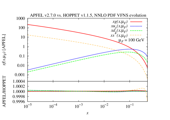
We start with the DGLAP PDF evolution in the VFN scheme with $\overline{\rm MS}$ heavy-quark thresholds. A careful benchmark was already presented in the original APFEL publication. In particular, the APFEL evolution has been checked against the HOPPET code Salam:2008qg v1.1.5, finding a very good agreement at the $\mathcal{O}\left(10^{-4}\right)$ level or better. Since then, APFEL has undergone several changes and improvements and thus we repeated the benchmark using the same settings and finding the same level of agreement with HOPPET, as shown in Fig. 1 for a representative set of combinations of PDFs.

Figure 1: Comparison between APFEL v2.7.0 and HOPPET v1.1.5 for the VFNS DGLAP evolution at NNLO with $\overline{\rm MS}$ heavy-quark thresholds. The evolution settings, $i.e.$ initial scale PDFs, reference value of $\alpha_{s}$, and heavy-quark thresholds, are the same as used in the Les Houches PDF evolution benchmark Dittmar:2005ed . The upper inset shows the gluon PDF $xg$, the valence up and down PDFs $xu_{v}\equiv xu-x\overline{u}$ and $xd_{v}\equiv xd-x\overline{d}$, respectively, and the total strangeness $xs^{+}\equiv xs+x\overline{s}$ at $\mu_{F}=100$ GeV as functions of the Bjorken variable $x$ as returned by APFEL. In the lower inset the ratio to HOPPET is displayed showing a relative difference of $10^{-4}$ or better all over the considered range.

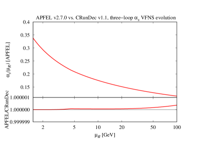
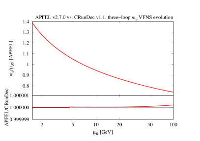
Although the benchmark of the DGLAP evolution already provides an indirect check of the evolution of $\alpha_{s}$, we have also performed a direct check of the VFNS evolution with $\overline{\rm MS}$ heavy-quark thresholds of $\alpha_{s}$ along with the evolution of the $\overline{\rm MS}$ charm mass. To this end, we have used the CRunDec code Schmidt:2012az , which is the C++ version of the Mathematica package RunDec Chetyrkin:2000yt . In Fig. 2 we show the comparison between APFEL and CRunDec for the three-loop evolution (NNLO) of the strong coupling $\alpha_{s}$ (left plot) and the charm mass $m_{c}$ (right plot). As is clear from the lower insets, the agreement between the two codes is excellent. Also the one- and two-loop evolutions have been checked finding the same level of agreement.

Figure 2: Comparison between APFEL v2.7.0 and CRunDec v1.1 for the VFNS RG three-loop evolution with $\overline{\rm MS}$ heavy-quark thresholds of the strong coupling $\alpha_{s}$ (left plots) and the $\overline{\rm MS}$ charm mass $m_{c}$ (right plot). The evolution settings are: $\alpha_{s}^{(n_{f}=3)}(\sqrt{2}\mbox{ GeV})=0.35$, $m_{c}^{(n_{f}=4)}(m_{c})=\sqrt{2}\mbox{ GeV}$, and $m_{b}^{(n_{f}=5)}(m_{b})=4.5\mbox{ GeV}$. The upper insets show the strong coupling $\alpha_{s}$ (left) and the charm mass $m_{c}$ (right) as functions of the renormalization scale $\mu_{R}$ as returned by APFEL. In the lower insets the ratios to CRunDec are displayed showing a relative difference well below $10^{-6}$ over the complete range considered.

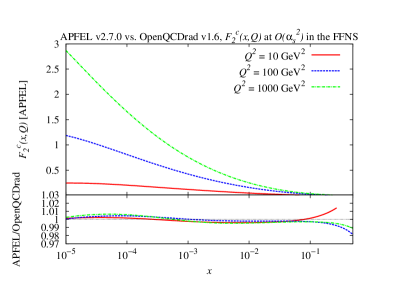
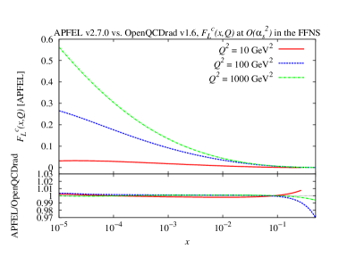
Finally, we benchmarked the implementation of massive DIS structure functions ($i.e.$ $F^{(3)}$ in eq. 1) with $\overline{\rm MS}$ masses against the public code OPENQCDRAD v1.6 openqcdrad . OPENQCDRAD implements DIS structure functions in terms of the $\overline{\rm MS}$ heavy-quark masses following the formalism discussed in Ref. Alekhin:2010sv . However, as already mentioned above, such a procedure does not directly correspond to what is needed for the implementation of the FONLL scheme. In order to make the comparison with OPENQCDRAD possible, we have implemented in APFEL a variant of the FONLL scheme with $\overline{\rm MS}$ masses where, as done in OPENQCDRAD , the RG running of the heavy-quark masses is expanded and truncated to the appropriate order. In Fig. 3 we show the comparison between APFEL and OPENQCDRAD for the exclusive charm neutral-current structure functions $F_{2}^{c}$ (left plot) and $F_{L}^{c}$ (right plot) at $\mathcal{O}(\alpha_{s}^{2})$ for three different values of $Q^{2}$ and over a wide range of $x$. As is clear from the lower ratio plots, the agreement is typically at the per-mil level except in the very large-$x$ region where, due to the smallness of the predictions, the relative difference tends to increase but maintains a good level of absolute accuracy.

Figure 3: Comparison between APFEL v2.7.0 and OPENQCDRAD v1.6 for the neutral-currents massive charm structure functions with $\overline{\rm MS}$ heavy-quark masses at $\mathcal{O}(\alpha_{s}^{2})$. As an input PDF set we have used MSTW2008nlo68cl_nf3 Martin:2010db from which also the numerical values of $\alpha_{s}$ and $m_{c}$ are taken. The upper insets show $F_{2}^{c}$ (left) and $F_{L}^{c}$ (right) as functions of $x$ for $Q^{2}=10,100,1000$ GeV² as returned by APFEL. In the lower insets the ratios to OPENQCDRAD are displayed showing a relative difference at the per-mil level except in the very large-$x$ region where, due to the smallness of the predictions, the relative differences tend to increase but maintain a good level of absolute accuracy.

To conclude this section, we observe that, referring to eq. (1), the introduction of the $\overline{\rm MS}$ masses does not affect the four-flavor structure function $F^{(4)}$. The structure function $F^{(3,0)}$ is instead affected by the transition from pole to $\overline{\rm MS}$ masses. Since we are not aware of any public code that computes such structure functions, a direct bechmark has not been possible. However, as a sanity check we have checked that $F^{(3,0)}$ and $F^{(3)}$ for large values of $Q^{2}$ tend to the same value, as the definition of $F^{(3,0)}$ requires.

3 QCD fit settings

The QCD fits were performed to the combined H1 and ZEUS charm production cross-section measurements Abramowicz:1900rp together with the combined HERA1+2 H1 and ZEUS inclusive DIS cross-section data Abramowicz:2015mha , accounting for all given sources of systematic uncertainties.

The kinematic region covered by HERA is constrained by the invariant mass of the hadronic system of $W>15$ GeV and the Bjorken scaling variable of $x<0.65$, therefore target mass corrections are expected to have negligible effects and are not discussed in this paper. The settings of the QCD fits in xFitter closely follow those used for the HERAPDF2.0 PDF extraction Abramowicz:2015mha , with a few differences related to the specifics of the current analysis which are motivated in the following.

The nominal result is extracted using the FONLL-C variant of the FONLL scheme discussed in Sect. 2. It should be pointed out that, while being accurate at NNLO for the inclusive DIS cross sections, the sensitivity to mass corrections of the FONLL-C scheme is actually NLO. The reason is that at $\mathcal{O}(\alpha_{s}^{0})$ the FONLL scheme reduces to the parton model which is insensitive to heavy-quark mass effects. Therefore, the first mass-sensitive term is $\mathcal{O}(\alpha_{s})$ which is the accuracy of the FONLL-A scheme which would thus provide a LO determination of the charm mass. Both the FONLL-B and the FONLL-C schemes, instead, include the $\mathcal{O}(\alpha_{s}^{2})$ massive corrections and thus would both produce determinations of the mass of the charm accurate at NLO. The advantage of FONLL-C with respect to FONLL-B is that it is accurate at $\mathcal{O}(\alpha_{s}^{2})$ also in the massless sector and thus it is supposed to provide a better description of the data. In other words, FONLL-C is the most accurate variant of the FONLL scheme presently available and as such it will be employed for our determination of $m_{c}(m_{c})$.

The result obtained in the FONLL scheme is accompanied by an analogous determination of $m_{c}(m_{c})$ obtained using the FFN scheme with $\overline{\rm MS}$ masses Alekhin:2013nda at NLO. Access to the structure functions calculated with the FFN scheme is possible via the xFitter interface to the OPENQCDRAD program openqcdrad using the QCDNUM program for the PDF evolution qcdnum .

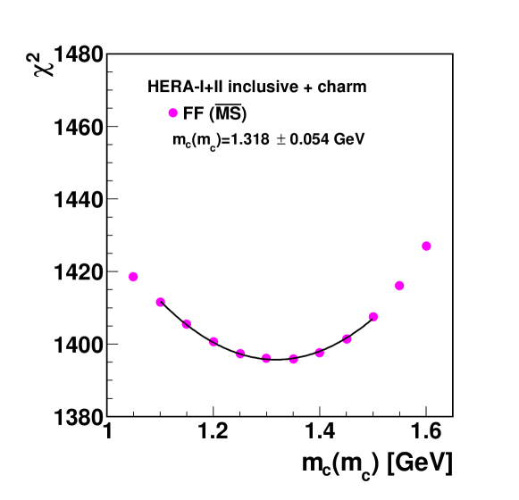
The procedure to determine the $\overline{\rm MS}$ charm mass follows closely the methodology described in Ref. Abramowicz:1900rp . It involves a series of fits in each of which a set of PDFs is determined corresponding to numerical values of charm mass ranging between $m_{c}(m_{c})=1.15$ GeV and $m_{c}(m_{c})=1.60$ GeV with steps of $0.05$ GeV. For each value of $m_{c}(m_{c})$ a value of global $\chi^{2}$ is obtained. The best fit value of $m_{c}(m_{c})$ is determined from the minimum of the parabolic fit to the resulting $\chi^{2}$ distribution and the associated 1-$\sigma$ uncertainty, which reflects the sensitivity of the data set to the charm mass, is determined as the $\Delta\chi^{2}=1$ variation around the minimum.

We now discuss the settings of the nominal fits and the variations that we performed to assess the different sources of uncertainty deriving from: the PDF parametrization, the model parameters, and the theoretical assumptions.

The assumption that heavy-quark PDFs are dynamically generated via gluon splitting at the respective thresholds requires that the starting scale $Q_{0}$ at which PDFs are parametrized is below the charm threshold, which in turn is identified with $m_{c}(m_{c})$. Given the range in which the scan of $m_{c}(m_{c})$ is done (from 1.1 to 1.6 GeV), we have chosen to set $Q_{0}=1$ GeV to allow all fits to be parametrized at the same starting scale. The combinations and the relative functional forms of the initial scale PDFs have been chosen following the parametrization scan procedure as performed for the HERAPDF2.0 determination Abramowicz:2015mha , and the optimal configuration has been found to be:

$$\begin{array}[]{rclcl}xg(x)&&&=&A_{g}x^{B_{g}}(1-x)^{C_{g}}-A^{\prime}_{g}x^{B^{\prime}_{g}}(1-x)^{25},\\ xu_{v}(x)&=&xu(x)-x\overline{u}(x)&=&A_{u_{v}}x^{B_{u_{v}}}(1-x)^{C_{u_{v}}}(1+E_{u_{v}}x^{2}),\\ xd_{v}(x)&=&xd(x)-x\overline{d}(x)&=&A_{d_{v}}x^{B_{d_{v}}}(1-x)^{C_{d_{v}}},\\ x\bar{U}(x)&=&x\overline{u}(x)&=&A_{\bar{U}}x^{B_{\bar{U}}}(1-x)^{C_{\bar{U}}}(1+D_{\bar{U}}x),\\ x\bar{D}(x)&=&x\overline{d}(x)+x\overline{s}(x)&=&A_{\bar{D}}x^{B_{\bar{D}}}(1-x)^{C_{\bar{D}}}.\end{array}$$ (79)

There are $14$ free parameters, since additional constraints were applied as follows. The QCD sum rules are imposed at the starting scale and constrain the normalisation parameters $A_{g}$, $A_{u_{v}}$, $A_{d_{v}}$. The light-sea quark parameters that affect the low-$x$ kinematic region $B_{\bar{U}}$ and $B_{\bar{D}}$, as well as the normalisation parameters $A_{\bar{U}}$ and $A_{\bar{D}}$, are constrained by the requirement that $\bar{u}\rightarrow\bar{d}$ as $x\to 0$, leading to the following constraints:

$$B_{\bar{U}} = B_{\bar{D}},$$ (80)

$$A_{\bar{U}} = A_{\bar{D}}(1-f_{s}),$$ (81)

with $f_{s}$ being the strangeness fraction of $\bar{D}$ assumed at the starting scale, $i.e.$ $f_{s}=\bar{s}/\bar{D}$, because HERA data alone are not able to provide a precise light-sea flavor separation. The strangeness fraction for the nominal fits is set to $f_{s}=0.4$, as in the HERAPDF2.0 analysis Abramowicz:2015mha .

In order to estimate the uncertainty associated to the PDF parametrization, we have considered the following variations with respect to the nominal configuration:

• we have moved up the initial scale $Q_{0}$ from 1 to $\sqrt{1.5}$ GeV. In the FONLL scheme, this restricted the $m_{c}(m_{c})$ range in which we did the scan because we could not use values of the charm mass such that $m_{c}(m_{c})<\sqrt{1.5}$ GeV. We were however able to perform the parabolic fit in order to find the best fit value of $m_{c}(m_{c})$. This complication does not arise in the FFN scheme in which there is no threshold crossing.

• In the $xu_{v}$ distribution we have included an additional linear term so that the last factor in second line of eq. (79) reads $(1+D_{u_{v}}x+E_{u_{v}}x^{2})$. After trying different variations of the parametrization, we found that this particular choice leads to the largest differences.

Moving to the model parameters, the values of the bottom and top quark masses for the nominal fits are chosen to be equal to the PDG values, defined in the $\overline{\rm MS}$ scheme, $i.e.$ $m_{b}(m_{b})=4.18$ GeV and $m_{t}(m_{t})=160$ GeV Agashe:2014kda . The value of the strong coupling is set to $\alpha_{s}(M_{Z})=0.118$. It should be pointed out that this value of $\alpha_{s}$ assumes 5 active flavors. For the FFN scheme fits, though, one needs to use the value of $\alpha_{s}$ with 3 active flavors. In order to find this value one has to evolve $\alpha_{s}(M_{Z})$ down to below $m_{c}(m_{c})$ in the VFN scheme and evolve back to $M_{Z}$ with 3 active flavors. We have computed the value of $\alpha_{s}$ with 3 active flavors for each of the values of $m_{c}(m_{c})$ considered.

The uncertainty associated to model parameters will be estimated by considering the following variations:

• the bottom mass has been moved up and down by 0.25 GeV, $i.e.$ $m_{b}(m_{b})=3.93$ GeV and $m_{b}(m_{b})=4.43$ GeV. The magnitude of the variation is actually much larger than the present uncertainty on the bottom mass and thus our choice is meant to provide a conservative estimate of the associated uncertainty.

• The variation of the strong coupling follows the recent PDF4LHC prescription Butterworth:2015oua . In particular, we have considered the conservative variation up and down by 0.0015 with respect to the nominal value, $i.e.$ $\alpha_{s}(M_{Z})=0.1165$ and $\alpha_{s}(M_{Z})=0.1195$.

• Finally, we considered the value of the strangeness fraction introduced in eq. (81) as being a model parameter and we have thus varied it up and down by 0.1 around the nominal value considering $f_{s}=0.3$ and $f_{s}=0.5$.

We finally turn to the theory assumptions and their variations. These mostly concern unknown higher-order corrections and the most common way to estimate them is by varying the renormalization and the factorization scales $\mu_{R}$ and $\mu_{F}$. As nominal scales in our analysis we have chosen $\mu_{R}^{2}=\mu_{F}^{2}=Q^{2}$ for both the FONLL and the FFN scheme analyses. Another possible source of theoretical uncertainty in the FONLL scheme is the presence of the damping factor discussed in Sect. 2 which is meant to suppress unwanted subleading terms and whose explicit form in the nominal fits is given in eq. (3).

The theoretical uncertainty associated to the missing higher-order corrections has been estimated as follows:

• the factorization and renormalization scales were varied by a factor 2 up and down with respect to the nominal values, that is choosing $\mu_{R}^{2}=\mu_{F}^{2}=Q^{2}/2$ and $\mu_{R}^{2}=\mu_{F}^{2}=2Q^{2}$. Such variations have been applied only to the heavy-quark components of the structure functions, while the light part has been left unchanged. The reason for this is that, in order to estimate the theoretical uncertainty associated to the determination of $m_{c}(m_{c})$, we want to perform scale variations only in the part of the calculation sensitive to this parameter, which is clearly the charm structure function (for consistency, the same variation was applied also to the bottom structure functions).

• As already mentioned, the FONLL damping factor represents a further source of uncertainty. It has the role of suppressing unwanted subleading terms but the particular way in which this suppression is implemented is somewhat arbitrary. To assess the impact of our particular choice on the determination of $m_{c}(m_{c})$, we have changed the suppression power around the nominal one, considering the following functional form:

  $$D_{p}(Q,m_{c})=\theta(Q^{2}-m_{c}^{2})\left(1-\frac{m_{c}^{2}}{Q^{2}}\right)^{p}\,,$$ (82)

  with $p=1,4$.

In addition, to assure the applicability of perturbative QCD and to keep higher-twist corrections under control, a cut on $Q^{2}$ is imposed on the fitted data. Our nominal cut is $Q^{2}>Q_{\rm min}^{2}=3.5$ GeV². The choice of the value of $Q_{\rm min}^{2}$ requires some care; an extensive discussion on the impact of varying it on the determination of $m_{c}(m_{c})$ is given in Sect. 4.3.

To conclude this section, we observe that the self-consistency of the input data set and the good control of the systematic uncertainties enable the determination of the experimental uncertainties in the PDF fits using the tolerance criterion of $\Delta\chi^{2}=1$.

4 Results

In this section we will present the result for our the determination of the value $m_{c}(m_{c})$ in the $\overline{\mbox{MS}}$ renormalization scheme using the FONLL scheme with its associated set of uncertainties.

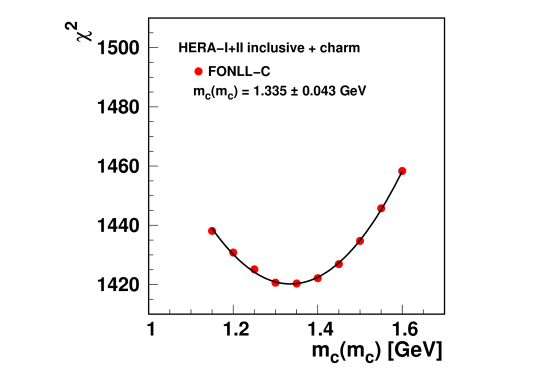
The parabolic fit to the global $\chi^{2}$ as a function of $m_{c}(m_{c})$ is shown in Fig. 4 and yields a best fit value and its 1-$\sigma$ experimental uncertainty equal to $m_{c}(m_{c})=1.335\pm 0.043$ GeV. An estimate of the parametric, model, and the theoretical uncertainties, performed following the procedure described in Sect. 3, is summarised in the second column of Tab. 1 and leads to our final result:

$$m_{c}(m_{c})=1.335\pm 0.043\mbox{(exp)}^{+0.019}_{-0.000}\mbox{(param)}^{+0.011}_{-0.008}\mbox{(mod)}^{+0.033}_{-0.008}\mbox{(th)}\mbox{ GeV.}$$ (83)

An illustration of the deviations, again determined through parabolic fits, caused by the variations employed to determine the parametric, model, and theoretical uncertainties is given in Fig. 5.

Figure 4: Parabolic fit to the global $\chi^{2}$ as a function of $m_{c}(m_{c})$ in the FONLL-C scheme with nominal settings.

variation	FONLL-C	FFN
central	$1.335\pm 0.043$	$1.318\pm 0.054$
$Q_{0}^{2}=1.5$	$1.354\;[+0.019]$	$1.329\;[+0.011]$
$D_{uv}$ non-zero	$1.340\;[+0.005]$	$1.308\;[-0.010]$
$f_{s}=0.3$	$1.338\;[+0.003]$	$1.320\;[+0.002]$
$f_{s}=0.5$	$1.332\;[-0.003]$	$1.315\;[-0.003]$
$m_{b}(m_{b})=3.93$ GeV	$1.330\;[-0.005]$	$1.312\;[-0.006]$
$m_{b}(m_{b})=4.43$ GeV	$1.343\;[+0.008]$	$1.324\;[+0.006]$
$\alpha_{s}(M_{Z})=0.1165$	$1.342\;[+0.007]$	$1.332\;[+0.014]$
$\alpha_{s}(M_{Z})=0.1195$	$1.329\;[-0.006]$	$1.300\;[-0.018]$
$\mu_{F}^{2}=\mu_{R}^{2}=2\cdot Q^{2}$	$1.347\;[+0.012]$	$1.314\;[-0.004]$
$\mu_{F}^{2}=\mu_{R}^{2}=Q^{2}/2$	$1.361\;[+0.026]$	$1.363\;[+0.045]$
FONLL Damping power = 1	$1.352\;[+0.017]$	–
FONLL Damping power = 4	$1.327\;[-0.008]$	–

Table 1: List of the variations performed to estimate the non-experimental uncertainties on $m_{c}(m_{c})$ with the respective results obtained in the FONLL-C scheme and in the FFN scheme at NLO.

Figure 5: Parabolic fits to the global $\chi^{2}$’s as functions of $m_{c}(m_{c})$ in the FONLL-C scheme for all variations performed to estimate the non-experimental uncertainties on $m_{c}(m_{c})$.

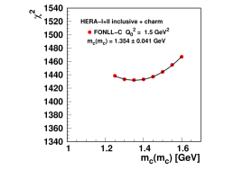
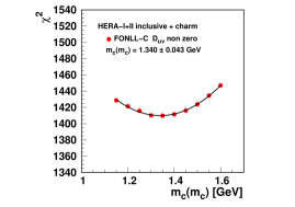
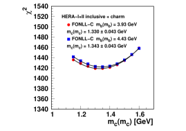
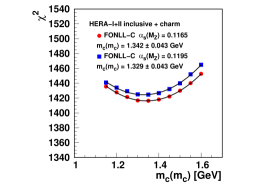
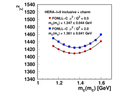
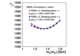
After we have determined the best fit value of the charm mass in eq. (83), we have used the central value to perform a further fit in the FONLL-C scheme (nominal fit). In Tab. 2 we report the partial $\chi^{2}$’s over the number of data points for each subset along with the total correlated $\chi^{2}$, the logarithmic penalty, and the total $\chi^{2}$ per degree of freedom.

Data Set	$\chi^{2}$
Charm cross section H1-ZEUS combined	44 / 47
HERA1+2 CCep	43 / 39
HERA1+2 CCem	55 / 42
HERA1+2 NCem	218 / 159
HERA1+2 NCep 820	67 / 70
HERA1+2 NCep 920	439 / 377
HERA1+2 NCep 460	220 / 204
HERA1+2 NCep 575	219 / 254
Correlated $\chi^{2}$	104
Log penalty $\chi^{2}$	+12
Total $\chi^{2}$ / d.o.f.	1420 / 1178

Table 2: $\chi^{2}$’s resulting from the fit in the FONLL-C scheme using the best fit value of the charm mass $m_{c}(m_{c})=1.335$ GeV. The partial $\chi^{2}$’s per data point along with the total correlated $\chi^{2}$, the logarithmic penalty, and the total $\chi^{2}$ / d.o.f. are reported, as defined in Ref. Aaron:2012qi .

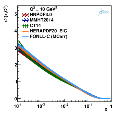
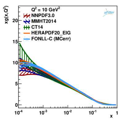
As an illustration, the singlet and the gluon PDFs extracted from the nominal fits are compared with other GM-VFNS PDF sets: CT14Dulat:2015mca , HERAPDF2.0Abramowicz:2015mha , MMHT14Thorne:2015caa , NNPDF3.0Ball:2014uwa . They are shown in Fig. 6 at the scale $Q^{2}=10$ GeV², where the the experimental uncertainties from the nominal fits on PDFs are estimated using Monte Carlo procedure with the root mean square estimated from 500 replica. An overall good agreement is observed.

Figure 6: Comparison at $Q^{2}=10$ GeV² of the singlet (left plot) and gluon (right plot) distributions from the nominal FONLL-C fit with other PDF sets determined using GM-VFN schemes: HERAPDF2.0, CT14, MMHT14, NNPDF3.0.

The FONLL determination of $m_{c}(m_{c})$ presented above is supported by an analogous determination in the FFN scheme at NLO. The corresponding parabolic fit with the associated experimental uncertainty is shown in Fig. 7. Also in this case a full characterization of the non-experimental uncertainty has beed achieved by carrying out the same parametric, model, and theory variations (except for the variation of the damping factor which is specific of the FONLL scheme). The results of the variation in the FFN scheme are reported in the third column of Tab. 1. The final result is:

$$m_{c}(m_{c})=1.318\pm 0.054\mbox{(exp)}^{+0.011}_{-0.010}\mbox{(param)}^{+0.015}_{-0.019}\mbox{(mod)}^{+0.045}_{-0.004}\mbox{(th)}\mbox{ GeV}\,,$$ (84)

which is in agreement with the FONLL determination given in eq. (83).

Figure 7: Parabolic fit to the global $\chi^{2}$ as a function of $m_{c}(m_{c})$ in the FFN scheme at NLO with nominal settings.

It is interesting to notice that we observe a reduced scale dependence in the FONLL scheme as compared to the FFN scheme. We ascribe this effect to the fact that the leading contributions in the FONLL scheme involve both gluon- and quark-initiated processes; typically the contributions from gluon processes decrease with the scale, while the contributions from quark processes tend to increase. Conversely, the FFN scheme is mostly driven by gluon processes the contributions of which (along with $\alpha_{s}$) tend to be monotonic in $\mu$ leading to larger scale variations.

As discussed Sect. 2.1.3, the running of the $\overline{\mbox{MS}}$ heavy-quark masses in the VFN scheme, exactly like the running of $\alpha_{s}$ and PDFs, is not univocally defined at the heavy-quark thresholds due to the presence of the so-called matching conditions. In particular, when giving the value of the mass at one of the heavy-quark thresholds, one should also specify whether this corresponds to the value immediately below or above the threshold itself. This is typically done by complementing the value with the number of active flavors used in the computation. In fact, in general $m_{c}^{(N_{f}=3)}(m_{c})\neq m_{c}^{(N_{f}=4)}(m_{c})$. On theoretical grounds, this difference is relevant when comparing a determination obtained in a VFN scheme like FONLL with a determination obtained in the ($N_{f}=3$) FFN scheme: in the latter one automatically determines $m_{c}^{(N_{f}=3)}(m_{c})$, while in the former it is more natural to extract $m_{c}^{(N_{f}=4)}(m_{c})$. However, eqs. (25) and (26) tell us how the two values are connected up to $\mathcal{O}(\alpha_{s}^{2})$ and applying eq. (25) to the central value eq. (83) one gets $m_{c}^{(N_{f}=3)}(m_{c})=1.339$ GeV, that is a difference of 0.004 GeV as compared to the nominal value which is well within the current uncertainty on $m_{c}(m_{c})$. We can then conclude that, even though providing a value $m_{c}(m_{c})$ is ambiguous if the number of active flavors is not specified, the magnitude of the ambiguity is currently not large enough to significantly affect the current determinations.

4.1 Comparison to other results

It is interesting to compare our results with the past determinations of $\overline{\mbox{MS}}$ charm mass $m_{c}(m_{c})$ using a similar methodology (also see Ref. Behnke:2015qja ; Alekhin:2013qqa ; Gao:2013wwa for previous comparisons).

The analysis of Ref. Alekhin:2012vu was performed in the ABM11 framework Alekhin:2012ig using the FFN scheme at NLO and at approximate NNLO and based on world data for DIS from HERA, and fixed-target DIS experiments and Tevatron Drell-Yan data. While the analysis in Ref. Alekhin:2012vu was performed including the same exclusive charm cross-section data used in this study, it did not include the HERA1+2 combined inclusive cross-section data set which was not available at the time, but used instead the HERA combined data from run 1 only. An earlier analysis Alekhin:2012un used a partial charm dataset only, with correspondingly larger uncertainties, while a subsequent analysis Alekhin:2013qqa investigated the correlation between the measurement of $m_{c}(m_{c})$ and the strong coupling constant.

The analysis of Ref. Gao:2013wwa is instead based on the CT10NNLO global analysis, and uses the S-ACOT-$\chi$ GM-VFN scheme discussed, $e.g.$, in Ref. Guzzi:2011ew . It is based on a slightly wider data set as it includes LHC jet production data and also a set of older $F_{2}^{c}$ measurements at HERA Adloff:2001zj that are not included in the more recent combined charm data. The authors of Ref. Gao:2013wwa provide a set of four determinations deriving from different strategies to convert the pole-mass definition into $\overline{\mbox{MS}}$. They also provide a separate estimate of the uncertainty due to the $\mathcal{O}(\alpha_{s}^{3})$ corrections for one of the four strategies essentially by varying the parameter that governs a generalized version of the rescaling variable $\chi$.

Finally, a determination of the charm mass $m_{c}(m_{c})$ was produced by the H1 and ZEUS collaborations in the framework of the HERAPDF QCD analysis in the same publication in which the charm cross-section measurements employed in our study were presented Abramowicz:1900rp . That determination also used only the HERA combined inclusive data from run 1 Aaron:2009aa .

In Tab. 3 we report the numerical values for the $m_{c}(m_{c})$ determinations listed above along with our results and the world average value PhysRevD.86.010001 . A short clarification about the nomenclature of the uncertainties reported in Tab. 3 is in order. In Sect. 3 we discussed extensively the meaning of the uncertainties associated to our determinations. In doing so, we tried to be consistent with the previous determinations, nevertheless some differences remain. As far as the determination in Ref. Abramowicz:1900rp is concerned, while their definition of “(exp)” and “(param)” essentially coincides with ours, their “(model)” uncertainty includes the variation of the cut in $Q^{2}$ (that we will discuss separately in Sect. 4.3) but does not include the $\alpha_{s}$ variation, which is instead quoted separately. In addition, the authors do not quote any scale variation uncertainty. The nomenclature of Ref. Alekhin:2012vu is also different from ours. Apart from the common “(exp)” uncertainty, for the NLO determination the authors only quote the “(scale)” uncertainty, which essentially coincides with our “(th)” (even though the FONLL “(th)” uncertainty also accounts for the variation of the damping factor), while for the approximate NNLO determination they also quote a “(th)” uncertainty which, differently from our nomenclature, accounts for the uncertainty on the approximated expressions used at $\mathcal{O}(\alpha_{s}^{3})$. Finally, the determinations in Ref. Gao:2013wwa only quote the experimental uncertainty (the asymmetric uncertainties are due to the use of a generic second-degree polynomial to fit the $\chi^{2}$ profiles). A graphical representation of Tab. 3 is shown in Fig. 8 where the inner error bars display the experimental uncertainty while the outer error bars (when present) are obtained as a sum in quadrature of all uncertainty sources. The blue vertical band represents the world average and provides a reference for all other determinations. It is clear that, while the spread of the current determinations of $m_{c}(m_{c})$ from DIS data covers a pretty large range, they are generally in agreement with the world average. As far as our determinations in particular are concerned, we observe that, apart from being consistent with each other and with the world average, they also present competitive uncertainties. This is particularly relevant for the FONLL determination because this is the first time that this scheme is employed for a direct determination of the charm mass.

scheme	$m_{c}(m_{c})$ [GeV]
FONLL (this work)	$1.335\pm 0.043\mbox{(exp)}^{+0.019}_{-0.000}\mbox{(param)}^{+0.011}_{-0.008}\mbox{(mod)}^{+0.033}_{-0.008}\mbox{(th)}$
FFN (this work)	$1.318\pm 0.054\mbox{(exp)}^{+0.011}_{-0.010}\mbox{(param)}^{+0.015}_{-0.019}\mbox{(mod)}^{+0.045}_{-0.004}\mbox{(th)}$
FFN (HERA) Abramowicz:1900rp	$1.26\pm 0.05\mbox{(exp)}\pm 0.03\mbox{(mod)}\pm 0.02\mbox{(param)}\pm 0.02(\alpha_{s})$
FFN (Alekhin et al.) Alekhin:2012vu	$1.24\pm 0.03({\rm exp})^{+0.03}_{-0.02}({\rm scale})^{+0.00}_{-0.07}({\rm th})$ (approx. NNLO)
	$1.15\pm 0.04({\rm exp})^{+0.04}_{-0.00}({\rm scale})$ (NLO)
S-ACOT-$\chi$ (CT10) Gao:2013wwa	$1.12^{+0.05}_{-0.11}$ (strategy 1)
	$1.18^{+0.05}_{-0.11}$ (strategy 2)
	$1.19^{+0.06}_{-0.15}$ (strategy 3)
	$1.24^{+0.06}_{-0.15}$ (strategy 4)
World average PhysRevD.86.010001	$1.275\pm 0.025$

Table 3: List of the recent determinations of $m_{c}(m_{c})$ from fits to DIS data along with the determinations extracted in this work. The PDG world average value is also reported for reference.

Figure 8: Graphical representation of the determinations reported in Tab. 3. The inner error bars display the experimental uncertainty while the outer error bars (when present) are obtained as a sum in quadrature of all uncertainty sources. The blue vertical band represents the world average and provides a reference for all other determinations.

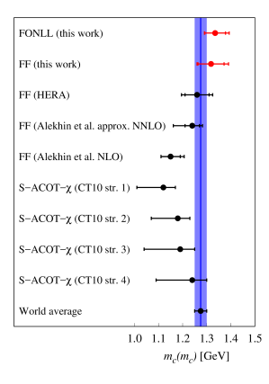
Fig. 8 shows that our determinations tend to be larger than the world average while most of the previous determinations place themselves below it. Detailed investigations show that the largest contribution to this difference arises from the use of to the new combined HERA1+2 combined inclusive cross section measurements that are employed for the first time to determine the charm mass and that, as we will discuss in Sect. 4.3, tend to prefer larger values of $m_{c}(m_{c})$.

4.2 Cross-checks

It is worth mentioning that we have also employed the variants A and B of the FONLL scheme discussed in Sect. 2 to determine $m_{c}(m_{c})$. While the FONLL-A scheme is accurate to LO in the massive sector and thus does not produce a reliable determination of the charm mass, the FONLL-B has the same formal accuracy in the massive sector as FONLL-C and indeed it leads to a determination comparable to that given in eq. (83) both for the central value and the uncertainties. It is interesting to notice that the FONLL-B scheme in the low-energy region resembles very closely the FFN scheme at NLO. In particular, both schemes are accurate to $\mathcal{O}(\alpha_{s}^{2})$ in the massive sector and to $\mathcal{O}(\alpha_{s})$ in the light sector. As a matter of fact, we find that the experimental uncertainty associated to the FONLL-B determination is very close to the FFN one quoted in eq. (84), which in turn is around 20% larger than that associated to the FONLL-C determination. This suggests that the $\mathcal{O}(\alpha_{s}^{2})$ corrections to the light sector that are present in the FONLL-C scheme, which depend on the heavy-quark mass by means of diagrams in which a gluon plits into a pair of heavy quarks, provide a further constraint on $m_{c}(m_{c})$.

Finally, we have also attempted a determination in the FFN scheme using the approximate NNLO massive structure functions as implemented in OPENQCDRAD. However, we did not pursue a full characterization of the uncertainties because we believe that this determination, while giving a quantitative indication of the effect of the NNLO corrections, cannot claim an NNLO accuracy and thus does not add anything to our NLO determinations.

4.3 Discussion on the $Q_{\rm min}^{2}$ dependence of the mass determination

Our determination of $m_{c}(m_{c})$ given in eq. (83) was obtained cutting off all data with $Q^{2}<Q_{\rm min}^{2}=3.5$ GeV². The necessity of such a cut stems from the fact that low-energy data are hard to describe for two main reasons: the large value of $\alpha_{s}$ with consequent large higher-order corrections, and sizable higher-twist corrections. In addition, as pointed out in Ref. Caola:2009iy , the low-$Q^{2}$ region (low-$x$, in fact) might be affected by deviations from the fixed-order DGLAP evolution whose description might require small-$x$ perturbative resummation. The dependence on $Q_{\rm min}^{2}$ of fits to HERA data has already been discussed in the context of the inclusive measurements only. In this section, we will address this issue considering also the HERA charm production data.

The particular value of $Q_{\rm min}^{2}$ used in our analysis (3.5 GeV²) was determined by requiring a good fit quality but maintaining a good sensitivity to $m_{c}(m_{c})$. This is illustrated in Fig. 9 where the global $\chi^{2}$ per degree of freedom is plotted as a function of $Q_{\rm min}^{2}$ in the left panel while the best fit of $m_{c}(m_{c})$ is plotted as a function of $Q_{\rm min}^{2}$ in the right panel. Looking at the left panel it is clear that, as expected, the global $\chi^{2}$ improves as more and more low-energy data are excluded from the fit. On the other hand, the right plot shows that the experimental uncertainty associated to $m_{c}(m_{c})$ gets larger and larger as $Q_{\rm min}^{2}$ increases indicating that, again as expected, the sensitivity to $m_{c}(m_{c})$ deteriorates if low-energy data are excluded. In the light of the plots in Fig. 9, we conclude that $Q_{\rm min}^{2}=3.5$ GeV² represents a good compromise between a good description of the full data set and a good sensitivity to $m_{c}(m_{c})$.

Figure 9: Left plot: dependence of the global $\chi^{2}$ / d.o.f. as a function of $Q_{\rm min}^{2}$. Right plot: dependence of the global best fit value of $m_{c}(m_{c})$ with the associated experimental uncertainty as a function of $Q_{\rm min}^{2}$. Both plots have been obtained using the FONLL-C scheme.

In this context, it is interesting to look at the behaviour of the partial $\chi^{2}$’s as a function of $Q_{\rm min}^{2}$ of the charm and inclusive cross-section data separately to assess in a more specific way which nominal value of $Q_{\rm min}^{2}$ is more convenient. Since the meaning of “degrees of freedom” is unclear for a subset of the full data set, in order to quantify the degree of improvement in the partial $\chi^{2}$’s, we consider the following quantity:

$$\frac{\Delta\chi^{2}}{\Delta N_{\rm points}}(Q_{\rm min}^{2})=\frac{\chi^{2}(Q_{\rm min}^{2})-\chi^{2}(Q_{\rm min}^{2}=2.5\mbox{ GeV}^{2})}{N_{\rm points}(Q_{\rm min}^{2})-N_{\rm points}(Q_{\rm min}^{2}=2.5\mbox{ GeV}^{2})}\,,$$ (85)

which provides an estimate of the improvement of the $\chi^{2}$ per data point with respect to our lowest cut $Q_{\rm min}^{2}=2.5$ GeV². If for a given value of $Q_{\rm min}^{2}$ this quantity is larger than one, this means that that specific cut leads to an improvement of the $\chi^{2}$ which is larger than the degrees of freedom subtracted by excluding a given number of data points and thus the excluded data points with respect of the reference cut (2.5 GeV²) are poorly described. On the contrary, if the quantity in eq. (85) is smaller than one, this means that the excluded data points are better described than the fitted ones. In the left panel of Fig. 10 we show the behaviour of the contribution to the global $\Delta\chi^{2}/\Delta N_{\rm points}$ originating from the charm data points only. It is clear that any cut between 3.5 and 5 GeV² improves drastically the partial $\chi^{2}$ while cuts above 5 GeV² either cause a much less significant improvement or even lead to a deterioration. This provides a further confirmation of the fact that our nominal cut (3.5 GeV²) is a sensible choice.

It is also interesting to look at the best fit values of $m_{c}(m_{c})$ and the relative uncertainty preferred by a given subset as a function of $Q_{\rm min}^{2}$ to quantify the sensitivity to $m_{c}(m_{c})$ as more and more data are excluded from the fit. This is plotted in the right panel of Fig. 10 for the charm cross-section data. It is clear that this particular subset of data tends to prefer values of $m_{c}(m_{c})$ around 1.23 GeV which is substantially lower than the global value given in eq. (83). The stability of the central value of $m_{c}(m_{c})$ for different values of $Q_{\rm min}^{2}$ is remarkable and, as expected, the experimental uncertainty tends to increase for larger value of $Q_{\rm min}^{2}$ indicating a loss of sensitivity.

Figure 10: Left plot: dependence of $\Delta\chi^{2}/\Delta N_{\rm points}$ as a function of $Q_{\rm min}^{2}$ for the charm cross-section subset. Right plot: dependence of the best fit value of $m_{c}(m_{c})$ with the associated experimental uncertainty as a function of $Q_{\rm min}^{2}$ for the charm cross-section subset in the combined fit. Both plots have been obtained using the FONLL-C scheme.

Finally, we have done the same exercise for the HERA1+2 inclusive cross-section data and in Fig. 11 we present the relative plots. In the left panel we observe that the $\chi^{2}$ of this subset improves essentially monotonically as $Q_{\rm min}^{2}$ increases while from the right panel it is clear that the preferred value of $m_{c}(m_{c})$ of the inclusive cross sections is substantially larger than that preferred by the charm cross sections with, again, uncertainties than become broader for larger values of $Q_{\rm min}^{2}$. It is finally clear that our best value for $m_{c}(m_{c})$ quoted in eq. (83) is a compromise between the lower value preferred by the exclusive charm data and the larger value preferred by the inclusive data.

Figure 11: Same as Fig. 10 for the inclusive cross-section subset in the combined fit.

4.4 Discussion on the sensitivity to $m_{c}(m_{c})$ of the inclusive data

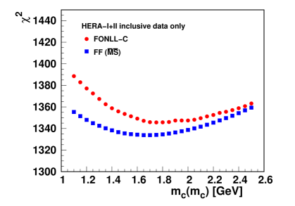
It is clear from the right panels of Figs. 10 and 11 that the exclusive charm and inclusive data subsets prefer somewhat different values of $m_{c}(m_{c})$. However, the values shown in these figures are clearly correlated because they were obtained in a simultaneous fit to all data. In order to investigate a possible tension, we have performed a fit to the inclusive data only using both the FONLL-C and FFN schemes. The $\chi^{2}$ profiles are shown in Fig. 12. In contrast to Figs. 4 and 7, in both schemes the scan in $m_{c}(m_{c})$ of the fits to inclusive data only yielded a shallow $\chi^{2}$ dependences with a minimum around $1.7$ GeV. This demonstrates that the inclusive data alone cannot constrain $m_{c}(m_{c})$ reasonably well, but also why this data exerts an upwards pull on the $m_{c}(m_{c})$ value in the combined fit. Furthermore, since Figs. 9, 10, and 11 in Sect. 4.3 present an overall remarkable stability of the central value of $m_{c}(m_{c})$ for different values of $Q^{2}_{\rm min}$, the observed feature cannot be attributed to the low $Q^{2}$ part of the inclusive data.

Figure 12: $\chi^{2}$ vs. $m_{c}(m_{c})$ profile for the fits to the HERA1+2 inclusive cross sections only. The red circles indicate the FONLL-C scheme while the blue squares the FFN scheme at NLO.

5 Conclusions

In this work we have presented a new determination of the $\overline{\rm MS}$ charm quark mass $m_{c}(m_{c})$ obtained by fitting HERA charm and inclusive DIS data. In particular, we included in our fits the combined H1 and ZEUS charm production cross-section measurements Abramowicz:1900rp and the final combination of HERA1+2 H1 and ZEUS inclusive DIS cross-section data Abramowicz:2015mha , the latter being used in this work for the first time for the extraction of the charm mass. Our determination is based on the FONLL general-mass variable-flavor-number scheme, and has required the generalization of the FONLL structure functions, originally constructed in the pole-mass scheme, in terms of $\overline{\rm MS}$ heavy quark masses.

A detailed estimate of the various sources of uncertainty that affect our determination of $m_{c}(m_{c})$ has been performed. In particular, we estimated the uncertainties due to the choice of the PDF parametrization, the model parameters used as input for the theoretical computations, and the missing higher-order corrections. We found that those sources of uncertainty are smaller than the experimental uncertainty, resulting in a competitive determination of the charm mass.

We complemented the FONLL extraction of the charm mass with an analogous determination based on the fixed-flavour number scheme at next-to-leading order, finding a good agreement between the two. In addition, we compared our results with previous determinations also based on fits to DIS data and with the PDG world average finding again a generally good agreement. We find that the values extracted in this work, although compatible within uncertainties, tend to be slightly higher than previous determinations from HERA data. This feature seems to be associated to the final HERA1+2 combined inclusive dataset, which tends to prefer larger values of $m_{c}(m_{c})$ as compared to the charm structure function data, and thus increases the best-fit value.

In the future, it would be interesting to repeat the FONLL determination in the context of a global PDF analysis, since, in addition to the inclusive and charm HERA data, other experiments are expected to have some sensitivity to the value of the $\overline{\rm MS}$ charm mass. In addition, the use of a wider dataset might lead to a reduction of the experimental uncertainties of the $m_{c}(m_{c})$ determination. Moreover, our analysis is based on the standard assumption that the charm PDF is dynamically generated by collinear splitting from gluons and light quarks. In this respect, it would be useful to redo the determination of $m_{c}(m_{c})$ in the presence of a possible non-perturbative charm PDF, for which the generalized FONLL structure functions accounting for a fitted heavy quark PDF are available Ball:2015tna .