Geometric integrator for simulations in the canonical ensemble

Abstract

In this work we introduce a geometric integrator for molecular dynamics simulations of physical systems in the canonical ensemble. In particular, we consider the equations arising from the so-called density dynamics algorithm with any possible type of thermostat and provide an integrator that preserves the invariant distribution. Our integrator thus constitutes a unified framework that allows the study and comparison of different thermostats and of their influence on the equilibrium and non-equilibrium (thermo-)dynamic properties of the system. To show the validity and the generality of the integrator, we implement it with a second-order, time-reversible method and apply it to the simulation of a Lennard-Jones system with three different thermostats, obtaining good conservation of the geometrical properties and recovering the expected thermodynamic results.

I Introduction

While dynamics in the microcanonical ensemble is easily generated from the standard Hamilton equations of motion for a conservative system, a problem arises when trying to generate deterministic equations of motion that reproduce a given system in contact with a thermal reservoir at a fixed temperature, i.e. a system in the canonical ensemble. This problem is relevant, for example, for molecular dynamics simulations, since the canonical ensemble is more useful for comparison with experimental situations allen1989computer ; rapaport2004art ; frenkel1996understanding . Several algorithms for simulations in the canonical ensemble have been suggested in the literature TuckermanBook ; leimkuhler2015molecular ; here, we focus on those that extend the physical phase space of the system of interest by adding an extra dimension which takes into account the interaction of the system with the environment. Such methods are usually referred to as thermostat algorithms, the most well-known being Nosé-Hoover dynamics evans1985thermostat ; hoover1985canonical .

It is known that several possible inequivalent deterministic thermostats correctly generate the canonical ensemble in the physical phase space jellinek1988generalization ; jellinek1988dynamics ; kusnezov1990canonical . Fukuda and Nakamura fukuda2002tsallis provided an algorithm called Density Dynamics (DD) that can generate, in principle, any invariant distribution in the extended and in the physical phase space. For example, Nosé-Hoover dynamics corresponds, in this scheme, to prescribing a Gaussian distribution for an extended variable that controls the interaction between the system and the environment. However, this choice is not unique: choosing a different distribution for the extended variable can also lead to a canonical ensemble in the physical phase space.

Recently, two of the present authors introduced a similar algorithm, Contact Density Dynamics (CDD) bravtap2016 , in which the equations of motion stem from contact Hamiltonian mechanics bravcruztapias2016 . One can show that this algorithm leads to results equivalent to those of DD; see Section II.

Given the fact that a canonical ensemble in the physical phase space can be reproduced by means of different types of thermostatting dynamics, an interesting question arises as to whether one can distinguish between such thermostats and establish criteria to prefer one over the other, at least for particular systems. For example, one such criterion is the lack of ergodicity for some value of the thermostatting parameter or for different temperature ranges, which would lead to a dynamics that does not correctly reproduce the expected thermodynamic properties. Therefore, for instance, one would like to show that for a given system a thermostat is superior over another in that it produces the correct results for a wider range of the thermostatting parameter and of the external temperature. Such a problem can be addressed either with theoretical investigations or with reference to numerical simulations; for the latter, for consistent comparisons it is necessary to have a unified and general framework for the numerical integration of any thermostat dynamics. Moreover, this unique numerical integrator should be constructed to respect the relevant geometric structures of each different thermostat.

In this work we introduce a numerical integrator with the above prescribed properties. It is a geometric integrator (geometric in the sense of structure-preserving ezra2006integrators ) for the equations of motion of Density Dynamics, adapted to the simulation of a physical system in the canonical ensemble. We show that our integrator works for any choice of the thermostatting mechanism and thus applies to any canonically thermostatted dynamics. The integrator is constructed by splitting the vector field of the dynamics and composing the individual flows using the symmetric Trotter factorization mclachlan2002splitting ; mclachlan2006geometric ; leimkuhler2015molecular ; hairer2006geometric ; TuckermanBook .

To show the usefulness of our integrator, we use it to simulate a Lennard-Jones fluid with $256$ particles in the canonical ensemble within three different thermostatting schemes: the Gaussian (Nosé-Hoover) model, the quartic model of Fukuda and Nakamura fukuda2006construction , and the logistic model that we proposed in bravtap2016 . The results show that our integrator is suitable for performing numerical simulations with any of the thermostatting schemes, and that it maintains control over the invariant quantity throughout the simulation once equilibrium is reached. Furthermore, all three schemes generate results that are consistent with the canonical ensemble. This is of particular interest to perform simulations where the Nosé-Hoover method fails, or takes a long time to reach equilibrium, such as occurs for the harmonic oscillator hoover1985canonical ; cho1992ergodicity ; watanabe2007ergodicity ; legoll2007nonergodicity , and to compare the results obtained by different thermostatting schemes.

We remark that the main difference between our integrator and the one described by Fukuda and Nakamura is that in fukuda2006construction the authors built a numerical integrator in the $(2n+2)$-dimensional extended phase space, assuming that an unspecified splitting was given for the $(2n+1)$-dimensional vector field. Here, instead, we directly provide, for the first time, an explicit splitting for the $(2n+2)$-dimensional vector field.

II Density Dynamics in the canonical ensemble

The standard Hamilton equations imply the conservation of energy and consequently they generate a dynamics in the microcanonical ensemble. There are several proposals to produce non-Hamiltonian dynamics consistent with different ensembles hoover1985canonical ; kusnezov1990canonical ; tuckerman1992chains ; leimkuhler2015molecular . In this work, we consider the Density Dynamics (DD) algorithm, which provides dynamical equations that generate an arbitrary density $\rho({\bf p},{\bf q},\zeta)$ as the invariant distribution in a $(2n+1)$-dimensional phase space fukuda2002tsallis .

The DD equations are given by

$$\dot{q}_{i}=\frac{\partial\Theta({\bf p},{\bf q},\zeta)}{\partial p_{i}}\,,$$ (1)

$$\dot{p}_{i}=-\frac{\partial\Theta({\bf p},{\bf q},\zeta)}{\partial q_{i}}-\frac{\partial\Theta({\bf p},{\bf q},\zeta)}{\partial\zeta}\,{p}_{i}\,,$$ (2)

$$\dot{{\zeta}}=\sum_{i=1}^{n}p_{i}\frac{\partial\Theta({\bf p},{\bf q},\zeta)}{\partial p_{i}}-{n}\,,$$ (3)

where ${\bf p}$ and ${\bf q}$ are the mechanical variables of the physical system of interest and $\zeta$ is an additional variable associated with the degrees of freedom of the thermal reservoir. Here $\Theta({\bf p},{\bf q},\zeta)=-{\rm ln}\rho({\bf p},{\bf q},\zeta)$ and $i$ goes from $1$ to $n$, the number of degrees of freedom of the physical system. We take $\rho$ to be the product of two independent distributions,

$$\rho=\rho_{\rm sys}({\bf p},{\bf q})\rho_{\rm th}(\zeta)\,,$$ (4)

where the desired invariant distribution $\rho_{\rm sys}$ for the physical system is obtained by integrating out the unphysical degree of freedom $\zeta$ over the distribution $\rho_{\rm th}$ of the thermostat.

A further justification for DD can be given in terms of the geometrical setting provided by Contact Density Dynamics (CDD). In this framework, one derives the equations of motion from contact Hamiltonian mechanics bravcruztapias2016 ; see equations (11)–(13) in bravtap2016 . To recover (1)–(3) from CDD one fixes the contact Hamiltonian to be $h=\exp(\Theta/n)$ and rescales time according to $dt\mapsto h/n\,dt$.

Another important property of the system (1)–(3) is that it has an invariant function fukuda2006construction . To see this, it is convenient to extend the $(2n+1)$-dimensional phase space to one with dimensionality $2n+2$, denoted in this work as the Extended Phase Space (EPS), by addition of the new coordinate $\nu$, whose equation of motion is

$$\dot{\nu}=-\frac{{\rm{div}}({X})}{n}\,,$$ (5)

where $X$ is the vector field defining the system (1)–(3). A straightforward calculation shows that

$$\dot{\nu}=\dfrac{\partial\Theta({\bf p},{\bf q},\zeta)}{\partial\zeta}$$ (6)

and that, given a solution $\phi(t)$ of (1)–(3), the quantity

$$I_{\phi}(t)=\Theta(\phi(t))+n\nu(\phi(t))\,.$$ (7)

is constant with respect to time $t$ (i.e., $\dot{I}_{\phi}\equiv 0$) and thus is an invariant of the flow.

For performing simulations in the canonical ensemble, the distribution $\rho$ is factored out as in (4):

$$\rho({\bf p},{\bf q},\zeta)=\dfrac{\exp(-\beta H({\bf p},{\bf q}))}{\mathcal{Z}}f(\zeta)\,,$$ (8)

with $H({\bf p},{\bf q})$ the Hamiltonian of the physical system, $\beta$ a constant (the inverse of the temperature of the reservoir), $\mathcal{Z}$ the partition function and $f(\zeta)$ a distribution for the variable $\zeta$. Substituting the joint distribution (8) into equations (1)–(3) and using (6), we get the following equations of motion in the EPS:

$$\dot{q}^{i}=\beta\frac{\partial H({\bf p},{\bf q})}{\partial p_{i}}\,,$$

$$\dot{p}_{i}=-\beta\frac{\partial H({\bf p},{\bf q})}{\partial q^{i}}+\frac{f^{\prime}(\zeta)}{f(\zeta)}p_{i}\,,$$

$$\dot{\zeta}=\beta\sum_{i=1}^{n}\frac{\partial H({\bf p},{\bf q})}{\partial p_{i}}p_{i}-n\,,$$

$$\dot{\nu}=-\frac{f^{\prime}(\zeta)}{f(\zeta)}\,.$$

By rescaling the vector field as

$${X}\mapsto\frac{X}{\beta}\equiv X_{\rm EPS}\,,$$ (9)

which is equivalent to the scaling in time $t\mapsto\beta t$, we get a more natural form for the equations of motion, namely

$$\dot{q}^{i}=\frac{\partial H({\bf p},{\bf q})}{\partial p_{i}}\,,$$ (10)

$$\dot{p}_{i}=-\frac{\partial H({\bf p},{\bf q})}{\partial q^{i}}+\frac{f^{\prime}(\zeta)}{\beta f(\zeta)}p_{i}\,,$$ (11)

$$\dot{\zeta}=\sum_{i=1}^{n}\frac{\partial H({\bf p},{\bf q})}{\partial p_{i}}p_{i}-\frac{n}{\beta}\,,$$ (12)

$$\dot{\nu}=-\frac{f^{\prime}(\zeta)}{\beta f(\zeta)}\,.$$ (13)

Since $\beta$ is constant, such a rescaling in time changes neither the equilibrium properties of the system nor the integral curves of the vector field .

The invariant quantity (7) after rescaling reads

$$I_{\phi}(t)=H({\bf p}(\phi(t)),{\bf q}(\phi(t))-\dfrac{{\rm{ln}}f(\zeta(\phi(t))}{\beta}+\frac{n}{\beta}\nu(\phi(t))\,.$$ (14)

Finally, it can be shown that the dynamics (10)–(13) in the EPS has the invariant measure Tuckerman2001

$${\rm d}\mu=e^{n\nu}{\rm d}^{n}q{\rm d}^{n}p{\rm d}\zeta{\rm d}\nu\,,$$ (15)

which, using the conservation law (14), can be rewritten as

$${\rm d}\mu=e^{n\nu}\delta\left(H({\bf p},{\bf q})-\dfrac{{\rm{ln}}f(\zeta)}{\beta}+\frac{n}{\beta}\nu-C\right){\rm d}^{n}q{\rm d}^{n}p{\rm d}\zeta{\rm d}\nu\,,$$ (16)

where $C$ is a constant defined by the initial condition. From (16) a canonical distribution for the physical phase space follows after integration of the additional degrees of freedom $\zeta$ and $\nu$. Therefore, assuming ergodicity and provided there are no additional integrals of motion, the dynamics (10)–(13) dynamically generates the canonical ensemble Tuckerman2001 .

We remark that the role of the thermostat is codified in the function $f(\zeta)$ and that different choices of $f$ lead to different dynamics, which are all, in principle, consistent with the canonical ensemble. For example, choosing $f(\zeta)$ as a Gaussian distribution one obtains the Nosé-Hoover dynamics, choosing a quartic distribution one obtains the dynamics proposed in fukuda2006construction , and with a choice of a logistic distribution one obtains the dynamics introduced in bravtap2016 .

III Geometric Integration

In this section, we present the main result of this paper, i.e. a geometric numerical integrator for the flow (10)–(13) that applies to any possible choice for the thermostatting function $f(\zeta)$.

III.1 Splitting of the vector field

An integrator is called geometric if it preserves exactly one or more of the geometric properties of a system of differential equations mclachlan2006geometric . For example, symplectic integrators are suitable for the integration of systems in the microcanonical ensemble, as they conserve the symplectic form and hence the phase space volume exactly mclachlan2006geometric . Furthermore, even though the energy is not preserved exactly by the approximate dynamics, the errors are bounded along the integration; see leimkuhler2015molecular for details. So, it is a desirable property of an integrator to be geometric or structure-preserving ezra2006integrators .

We now present a geometric integrator for the system (10)–(13) with properties analogous to those of symplectic integrators for conservative systems, since it conserves the invariant measure (15) and maintains the error in the invariant quantity (14) bounded. The fulfillment of the first property can be examined analytically, while the second property is checked through numerical experiments.

To build the integrator we use the splitting method mclachlan2002splitting . The idea of this method is to decompose a vector field $X$ into vector fields $X_{i}$, with $X=\sum_{i}X_{i}$, such that each $X_{i}$ shares the same properties as $X$; the advantage is that the $X_{i}$s are easier to treat numerically. In our case, the property that we want to preserve with the splitting is the conservation of the invariant measure. For concreteness, since $X_{\rm EPS}$ given in (9) satisfies

$$\pounds_{X_{\rm EPS}}{\rm d}\mu=0\,,$$ (17)

where $\pounds$ is the Lie derivative (i.e. the derivative along the vector field $X_{\rm EPS}$ leimkuhler2015molecular ) and ${\rm d}\mu$ is given in (15), we require each vector field in the splitting $X_{\rm EPS}~{}=~{}\sum_{i}X_{i}$ to separately satisfy

$$\pounds_{X_{i}}{\rm d}\mu=0\,.$$ (18)

We begin by separating $X_{\rm EPS}$ into two parts,

$$X_{\rm EPS}=X_{\rm sys}+X_{\rm th}\,,$$ (19)

with $X_{\rm sys}$ the vector field associated with the Hamiltonian evolution of the physical system,

$$X_{\rm sys} =X_{\rm sys}^{1}+X_{\rm sys}^{2}$$ (20)

$$=\left[-\frac{\partial H(\bf{p},\bf{q})}{\partial q^{i}}\frac{\partial}{\partial{p_{i}}}\right]+\left[\frac{\partial H(\bf{p},\bf{q})}{\partial p_{i}}\frac{\partial}{\partial{q^{i}}}\right]$$ (21)

and $X_{\rm th}$ the vector field associated with the action of the thermostat,

$$\begin{split}X_{\rm th}{}&=X_{\rm th}^{1}+X_{\rm th}^{2}\end{split}$$ (22)

$$\begin{split}{}&=\left[\left(\sum_{i=1}^{n}\frac{\partial H(\bf{p},\bf{q})}{\partial p_{i}}p_{i}-\frac{n}{\beta}\right)\frac{\partial}{\partial{\zeta}}\right]\\ {}&+\left[\frac{g(\zeta)}{\beta}p_{i}\frac{\partial}{\partial{p_{i}}}-\frac{g(\zeta)}{\beta}\frac{\partial}{\partial\nu}\right]\,,\end{split}$$ (23)

where $g(\zeta)\equiv{{\rm d}{\rm ln}f(\zeta)}/{{\rm d}\zeta}$. It is easy to check that if the Hamiltonian of the physical system is of the form $H({\bf p},{\bf q})=K({\bf p})+V({\bf q})$, then

$$\pounds_{X_{\alpha}^{(i)}}{\rm d}\mu=0\quad\text{for}\quad\alpha={\rm sys,th}\quad\text{and}\quad i=1,2\,$$ (24)

and thus the individual vectors $X_{\rm sys}^{1},X_{\rm sys}^{2},X_{\rm th}^{1}$ and $X_{\rm th}^{2}$ provide the required splitting of $X_{\rm EPS}$.

We proceed with the composition of the individual flows generated by each vector field $X_{\alpha}^{i}$. There are different ways to perform such a composition; see e.g. mclachlan2002splitting ; mclachlan1995numerical . Here, we use a simple factorization scheme that is enough to illustrate the validity of our integrator.

III.2 Numerical algorithm

We recall that formally the flow $\phi_{\rm EPS}(t)$ defined by the vector field $X_{\rm EPS}$ is applied to an initial condition $\omega$ as leimkuhler2015molecular

$$\phi_{\rm EPS}(t)(\omega)=\exp(tX_{\rm EPS})(\omega)\,.$$ (25)

Since the right hand side of (25) cannot be evaluated analytically, we take advantage of the splitting of the previous section and of a particular method of composition in order to numerically integrate the dynamics (10)–(13). The method of composition that we use in this work is the symmetric Trotter factorization (also known as the Strang splitting formula or Suzuki’s 2nd order method) TuckermanBook ; hairer2006geometric ; ishida1998water , which is one of the simplest methods to implement a geometric algorithm and test its properties ezra2006integrators .

The Trotter factorization of the flow corresponding to the splitting (19), applied to a single time step $\tau$, is

$$\begin{split}\exp(\tau X_{\rm EPS})&=\exp\left(\frac{\tau}{2}X_{\rm th}\right)\exp(\tau X_{\rm sys})\exp\left(\frac{\tau}{2}X_{\rm th}\right)\\ &+\mathcal{O}(\tau^{3})\,.\end{split}$$ (26)

Applying again the Trotter factorization to the further splittings (20) and (22), we obtain

$$\begin{split}\exp(\tau X_{\rm EPS})=&\exp\left(\frac{\tau}{4}X_{\rm th}^{1}\right)\exp\left(\frac{\tau}{2}X_{\rm th}^{2}\right)\exp\left(\frac{\tau}{4}X_{\rm th}^{1}\right)\\ &\exp\left(\frac{\tau}{2}X_{\rm sys}^{1}\right)\exp(\tau X_{\rm sys}^{2})\exp\left(\frac{\tau}{2}X_{\rm sys}^{1}\right)\\ &\exp\left(\frac{\tau}{4}X_{\rm th}^{1}\right)\exp\left(\frac{\tau}{2}X_{\rm th}^{2}\right)\exp\left(\frac{\tau}{4}X_{\rm th}^{1}\right)\\ &+\mathcal{O}(\tau^{3})\,.\end{split}$$ (27)

Alternatively, the superscripts $1$ and $2$ may be exchanged, producing an equivalent algorithm.

From now on, we consider a mechanical system with Hamiltonian

$$H(\mathbf{p},\mathbf{q})=\sum_{i=1}^{n}\frac{p_{i}^{2}}{2m_{i}}+V(\bf{q})\,.$$ (28)

The flow defined by (27) applied to any initial condition $\omega$ starts with the evaluation of the operator $\exp\left(\frac{\tau}{4}X_{\rm th}^{1}\right)$, namely the translation

$$\exp\left(\frac{\tau}{4}X_{\rm th}^{1}\right)(\omega)=\exp\left(\frac{\tau}{4}\left(\sum_{i=1}^{n}\frac{p_{i}^{2}}{m_{i}}-\frac{n}{\beta}\right)\frac{\partial}{\partial{\zeta}}\right)\begin{pmatrix}q^{i}\\ p_{i}\\ \zeta\\ \nu\end{pmatrix}=\begin{pmatrix}q^{i}\\ p_{i}\\ \displaystyle\zeta+\frac{\tau}{4}\left(\sum_{i=1}^{n}\frac{p_{i}^{2}}{m_{i}}-\frac{n}{\beta}\right)\\ \nu\end{pmatrix}\,.$$ (29)

We proceed to evaluate ${\rm exp}(\frac{\tau}{2}X_{\rm th}^{2})$. Note that the components of $X_{\rm th}^{2}$ commute with each other. This allows us to apply directly the operator $\exp(\frac{\tau}{2}X_{\rm th}^{2})$ over the evolved initial condition without a further splitting, to obtain

$$\exp\left(\frac{\tau}{2}X_{\rm th}^{2}\right)\begin{pmatrix}q^{i}\\ p_{i}\\ \displaystyle\zeta+\frac{\tau}{4}\left(\sum_{i=1}^{n}\frac{p_{i}^{2}}{m_{i}}-\frac{n}{\beta}\right)\\ \nu\end{pmatrix}=\exp\left(\frac{\tau}{2}\left(\frac{g(\zeta)}{\beta}p_{i}\frac{\partial}{\partial{p_{i}}}-\frac{g(\zeta)}{\beta}\frac{\partial}{\partial\nu}\right)\right)\begin{pmatrix}q^{i}\\ p_{i}\\ \displaystyle\zeta+\frac{\tau}{4}\left(\sum_{i=1}^{n}\frac{p_{i}^{2}}{m_{i}}-\frac{n}{\beta}\right)\\ \nu\end{pmatrix}=$$

$$\exp\left(\frac{\tau}{2}\left(\frac{g(\zeta)}{\beta}p_{i}\frac{\partial}{\partial{p_{i}}}\right)\right)\begin{pmatrix}q^{i}\\ p_{i}\\ \displaystyle\zeta+\frac{\tau}{4}\left(\sum_{i=1}^{n}\frac{p_{i}^{2}}{m_{i}}-\frac{n}{\beta}\right)\\ \displaystyle\nu-\frac{\tau}{2}\left(\frac{g(\zeta)}{\beta}\right)\end{pmatrix}=\begin{pmatrix}q^{i}\\ \displaystyle p_{i}\exp\left(\frac{\tau}{2}\left(\frac{g(\zeta)}{\beta}\right)\right)\\ \displaystyle\zeta+\frac{\tau}{4}\left(\exp\left(\tau\frac{g(\zeta)}{\beta}\right)\sum_{i=1}^{n}\frac{p_{i}^{2}}{m_{i}}-\frac{n}{\beta}\right)\\ \displaystyle\nu-\frac{\tau}{2}\left(\frac{g(\zeta)}{\beta}\right)\end{pmatrix}\,,$$ (30)

where in the last equality we have used the identity $[\exp\left(cx\frac{\partial}{\partial x}\right)]f(x)=f(x\exp(c))$ TuckermanBook . Then we apply again the operator $\exp\left(\frac{\tau}{4}X_{\rm th}^{1}\right)$ to the evolved condition (III.2), obtaining

$$\begin{pmatrix}q^{i}\\ \displaystyle p_{i}\exp\left[\frac{\tau}{2}\left(\frac{g(\tilde{\zeta})}{\beta}\right)\right]\\ \displaystyle\tilde{\zeta}+\frac{\tau}{4}\left[\exp\left(\tau\frac{g(\tilde{\zeta})}{\beta}\right)\sum_{i=1}^{n}\frac{p_{i}^{2}}{m_{i}}-\frac{n}{\beta}\right]\\ \displaystyle\nu-\frac{\tau}{2}\left(\frac{g(\tilde{\zeta})}{\beta}\right)\end{pmatrix}\,,$$ (31)

with

$$\tilde{\zeta}=\zeta+\frac{\tau}{4}\left(\sum_{i=1}^{n}\frac{p_{i}^{2}}{m_{i}}-\frac{n}{\beta}\right)\,.$$ (32)

The set of equations (29), (III.2), (31) defines the first integral operator $L_{\rm th}(\tau)=\exp(\tau/2X_{\rm th})$ in (26), representing the action of the thermostat.

Now we proceed with the composition of the evolution operators of the vector fields associated to the physical system. A straightforward calculation shows that in our scheme the factorization

$$\exp(\tau X_{\rm sys})=\exp\left(\frac{\tau}{2}X_{\rm sys}^{1}\right)\exp(\tau X_{\rm sys}^{2})\exp\left(\frac{\tau}{2}X_{\rm sys}^{1}\right)$$ (33)

leads to the velocity Verlet algorithm, which is a standard second-order integrator for Hamiltonian systems TuckermanBook ; leimkuhler2015molecular ; we write $L_{\rm Verlet}(\tau)=\exp(\tau X_{\rm sys})$. Therefore we conclude that the total effect of the operator on the right hand side of (26) may be codified in the following composition for each time step $\tau$ and initial condition $\omega$

$$\left[L_{\rm th}(\tau)\circ L_{\rm Verlet}(\tau)\circ L_{\rm th}(\tau)\right](\omega)$$ (34)

which is our geometric algorithm for the integration of the equations (10)–(13). We remark that we recover the known integrator for Nosé-Hoover dynamics considered in ishida1998water ; ezra2006integrators . An extension of this factorization to a higher-order method may be obtained using the Suzuki-Yoshida scheme TuckermanBook .

IV Numerical experiments

In this section, we report the results of an implementation of our algorithm in the Julia language (available at julialennard ), to perform simulations of a $256$-particle Lennard-Jones fluid in 3 dimensions.

IV.1 Thermostat distributions

We use three different thermostat distributions $f(\zeta)$ for the dynamics (10)–(13), corresponding to the known different dynamics mentioned in the introduction. Namely, the Gaussian distribution, which yields the classical Nosé-Hoover dynamics, the logistic distribution, introduced in the context of Contact Density Dynamics bravtap2016 and the quartic distribution, considered by Fukuda and Nakamura in Density Dynamics fukuda2002tsallis . They are summarized in Table 1, together with the single free parameter associated to each one.

Distribution	$f(\zeta)$	Parameter
Gaussian	$\sqrt{\dfrac{\beta}{2\pi Q}}{\exp\left(-\dfrac{\beta\zeta^{2}}{2Q}\right)}$	${Q}$
Logistic	$\dfrac{\exp(\zeta-m)}{(1+\exp(\zeta-m))^{2}}$	$m$
Quartic	$\dfrac{2\Gamma(3/4)}{\sqrt{2}\pi c^{-1/4}}\exp(-c\,\zeta^{4})$	$c$

Table 1: Distributions $f(\zeta)$ used to perform molecular simulations. The parameter in the Gaussian distribution corresponds to the standard deviation, while in the logistic distribution it corresponds to the mean. The quartic distribution is a generalized Gaussian distribution with parameter $c$ related to the standard deviation nadarajah2005generalized .

IV.2 Methods and notation

We use a shifted-force potential allen1989computer with a cutoff distance $r_{c}^{*}=2.5$ (the superscript ^∗ denotes reduced units frenkel1996understanding ). In addition, we consider the system enclosed in a cubic box with periodic boundary conditions .

For comparison with experimental values, we take this potential as a model for argon. A time step $\Delta t^{*}=0.005$ (corresponding to a physical one of $\Delta t=11~{}\rm{fs}$) and a reduced density $\rho^{*}=0.8$ ($\rho=34~{}\rm{mol/L}$) are used. $N=256$ is the number of particles considered. $T_{\rm sys}^{*}$ refers to the instantaneous reduced temperature of the system

$$T_{\rm sys}^{*}=\frac{2\langle K^{*}\rangle}{3(N-1)}\,,$$ (35)

while $T_{\rm th}^{*}$ refers to the fixed temperature of the thermostat. The conversion factor between the reduced and physical temperature is $119.8~{}{\rm K}$. The simulations are carried out by setting the free parameters in the distributions to the values $Q=1.0$, $m=2.0$ and $c=0.1$.

Finally, we take an initial configuration with particles arranged in a cubic simulation cell containing 64 face-centered cubic unit cells and velocities determined by the Boltzmann distribution at temperature $T^{*}_{\rm th}$.

IV.3 Results

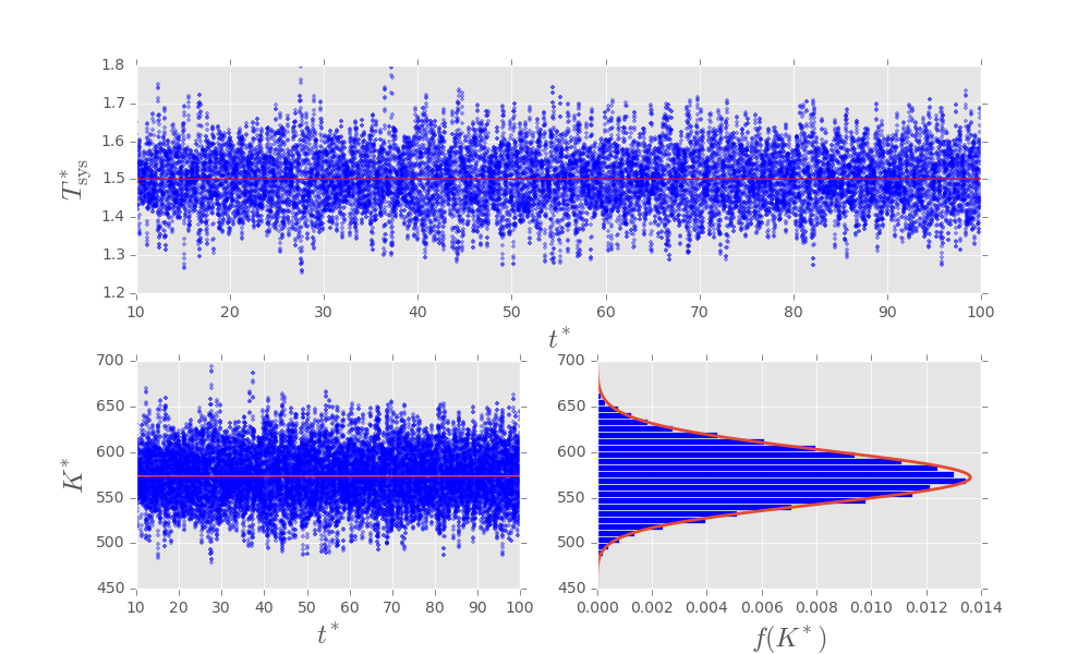
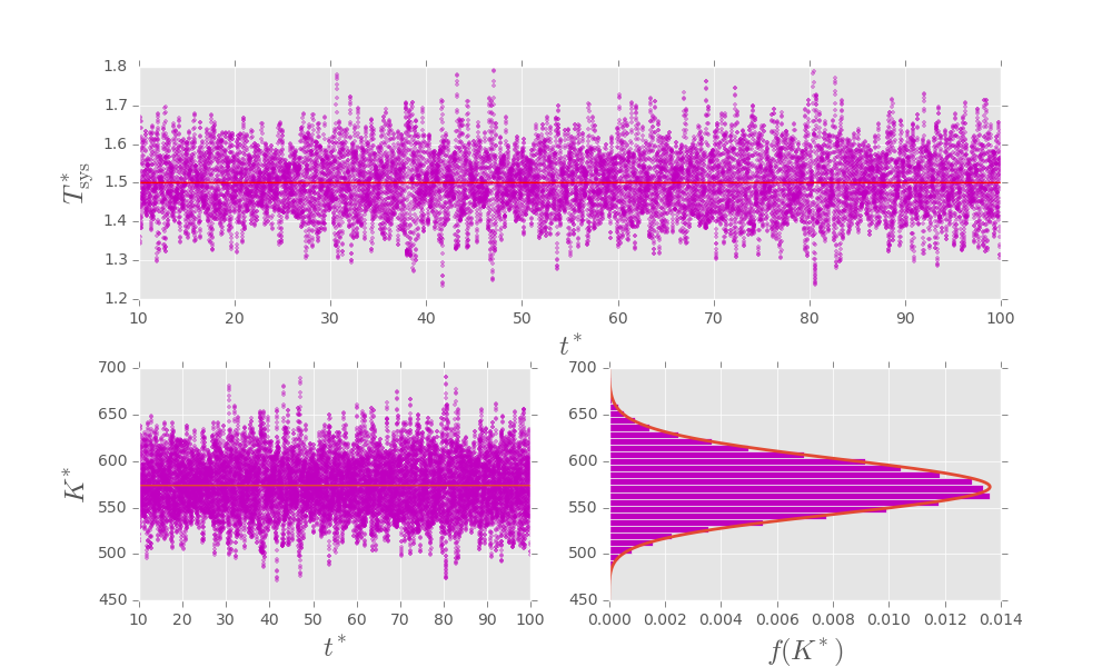
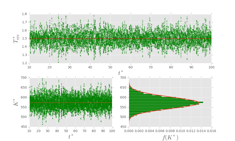
In figures 1, 2 and 3, we show the behaviour of $T_{\rm sys}^{*}$ with respect to time after equilibrium is reached for the three different thermostats. It is evident that $T_{\rm sys}^{*}$ fluctuates around a mean value that coincides with $T_{\rm th}^{*}$. We report also the behavior of the reduced kinetic energy and its numerical distribution compared to the theoretical one,

$$\rho(K^{*})=\dfrac{{\rm e}^{-\beta K^{*}}\left(K^{*}\right)^{\frac{3(N-1)}{2}-1}}{\beta^{\frac{3(N-1)}{2}}\Gamma\left(\frac{3(N-1)}{2}\right)}\,,$$ (36)

showing that the results agree with the theoretical expectations in all three cases.

Figure 1: Evolution of the reduced temperature of the system (35) at equilibrium with the Gaussian thermostat at a reduced temperature $T_{\rm th}^{*}=1.5$. We report also the behavior of the reduced kinetic energy $K^{*}$ and its numerical distribution $f(K^{*})$, compared with the theoretical one (36).

Figure 2: Evolution of the reduced temperature of the system (35) at equilibrium with the logistic thermostat at a reduced temperature $T_{\rm th}^{*}=1.5$. We report also the behavior of the reduced kinetic energy $K^{*}$ and its numerical distribution $f(K^{*})$, compared with the theoretical one (36).

Figure 3: Evolution of the reduced temperature of the system (35) at equilibrium with the quartic thermostat at a reduced temperature $T_{\rm th}^{*}=1.5$. We report also the behavior of the reduced kinetic energy $K^{*}$ and its numerical distribution $f(K^{*})$, compared with the theoretical one (36).

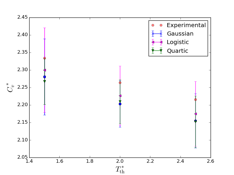
The fluctuations of the energy are used to determine the reduced heat capacity of the system according to

$$C_{v}^{*}=\frac{\langle(H^{*}-\langle H^{*}\rangle)^{2}\rangle}{N\langle T_{\rm sys}^{*}\rangle^{2}}\,,$$ (37)

where the average is performed with respect to time in the numerical simulation. In figure 4 we compare the results obtained with the tabulated values for argon under the same conditions . We display the mean values of $C_{v}^{*}$ for the three different temperatures analyzed, together with the corresponding standard deviation bars obtained using a sample of 50 simulations for each case. Clearly our results agree statistically with the experimental values.

Figure 4: Reduced heat capacities of each thermostatted dynamics at three different thermostat temperatures ($T_{\rm th}^{*}=1.5$, $T_{\rm th}^{*}=2.0$ and $T_{\rm th}^{*}=2.5$). The error bars represent the standard deviation of the result corresponding to 50 realizations of the simulation.

As a final test that the three different dynamics correctly reproduce the canonical ensemble, we calculate in each case the scaled covariance of the kinetic and the potential energy, defined as

$${\rm cov}^{*}(K,U)=\dfrac{\langle\Delta K^{*}\Delta U^{*}\rangle}{N\langle T^{*}_{\rm sys}\rangle^{2}}\,$$ (38)

with $\Delta Y=Y-\langle{Y}\rangle$ for $Y=U^{*},K^{*}$. This quantity is expected to vanish at equilibrium valenzuela2015 . In Table 2 we display the statistical results of covariances for samples of 50 simulations. They are in agreement with the expectation in all cases.

	$T_{\rm th}^{*}=1.5$		$T_{\rm th}^{*}=2.0$		$T_{\rm th}^{*}=2.5$
Reservoir	mean	std	mean	std	mean	std
Gaussian	$-6.22\times 10^{-4}$	$0.017$	$-1.67\times 10^{-3}$	$0.014$	$-6.76\times 10^{-4}$	$0.012$
logistic	$8.64\times 10^{-3}$	$0.025$	$5.73\times 10^{-3}$	$0.018$	$2.66\times 10^{-3}$	$0.014$
quartic	$-1.23\times 10^{-3}$	$0.015$	$1.00\times 10^{-4}$	$0.013$	$7.61\times 10^{-4}$	$0.008$

Table 2: Mean reduced covariances (mean) and standard deviations (std) of the kinetic and potential energy calculated with formula (38) for 50 simulations in each case under the specified conditions.

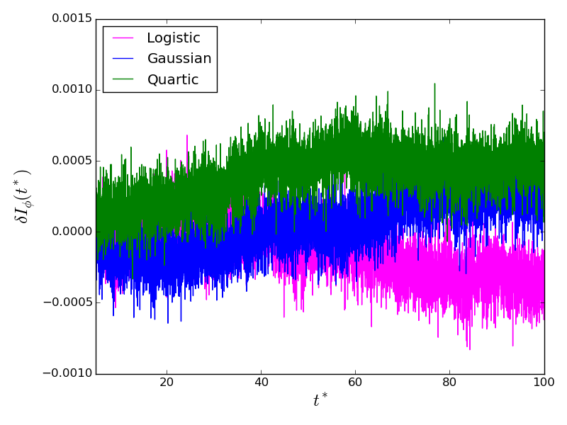
Additionally, to test the validity of the integrator, we keep track of the evolution of the invariant quantity (14) as the system is numerically integrated. Since the algorithm is constructed so as to preserve just the invariant measure, the invariant quantity is not necessarily preserved exactly by the approximate dynamics. However, its fluctuations are expected to be bounded and not to have any particular drift. Figure (5) confirms this expectation for the three thermostat dynamics considered.

Figure 5: Evolution of the relative error in the invariant $\delta I_{\phi}(t^{*})~{}=~{}\frac{I(t^{*})-I(t_{\rm eq}^{*})}{I(t_{\rm eq}^{*})}$ after equilibrium has been reached ($t_{\rm eq}^{*}=5.0$). A random simulation was chosen for the same reduced temperature $T^{*}_{\rm th}={1.5}$.

V Conclusions

In this work we have provided a new integrator for molecular dynamics simulations in the canonical ensemble. The main characteristics of our integrator are that it is geometric, in the sense that it preserves the invariant measure of the dynamics, and that it works for any type of thermostat within the density dynamics formalism. Different thermostatted dynamics may be generated according to equations (10)–(13) by specifying the distribution $f(\zeta)$ and they are all expected to give rise to a canonical ensemble, provided the ergodic assumption is fulfilled. Our algorithm provides a unified framework for the integration of all these thermostatted dynamics, and thus a useful tool for their comparison. In fact, while in principle the thermodynamic properties of the system do not depend on the subtleties of the thermostat algorithm, in practice there are issues that may cause a thermostat to be preferable over another. As an example, it is known for the Nosé-Hoover thermostat that the choice of $Q$ is an important factor for the correctness of the simulation cho1992ergodicity ; valenzuela2015 .

In order to obtain results that are consistent and comparable for simulations of different thermostatted dynamics, it is necessary to use the same integrator for all cases. Our integrator provides such a unified scheme to compare different canonical dynamics, as shown here, or even to extend the comparison to more sophisticated deterministic algorithms, such as Nosé-Hoover chains tuckerman1992chains .

Future work will be devoted to the implementation of the algorithm with higher-order methods, to the simulation of several physical systems and to the extension of the integrator to ensembles different from the canonical one.

References

- (1) M. P. Allen and D. J. Tildesley, Computer Simulation of Liquids. Oxford university press, 1989.
- (2) D. C. Rapaport, The Art of Molecular Dynamics Simulation. Cambridge university press, 2004.
- (3) D. Frenkel and B. Smit, Understanding Molecular Simulations: from Algorithms to Applications. 1996.
- (4) M. E. Tuckerman, Statistical Mechanics: Theory and Molecular Simulation. Oxford graduate texts, Oxford: Oxford University Press, 2010.
- (5) B. Leimkuhler and C. Matthews, Molecular Dynamics: with Deterministic and Stochastic Numerical Methods, vol. 39. Springer, 2015.
- (6) D. J. Evans and B. L. Holian, “The Nosé-Hoover thermostat,” The Journal of Chemical Physics, vol. 83, no. 8, 1985.
- (7) W. G. Hoover, “Canonical dynamics: equilibrium phase-space distributions,” Physical Review A, vol. 31, no. 3, p. 1695, 1985.
- (8) J. Jellinek and R. S. Berry, “Generalization of Nosé’s isothermal molecular dynamics,” Physical Review A, vol. 38, no. 6, p. 3069, 1988.
- (9) J. Jellinek, “Dynamics for nonconservative systems: ergodicity beyond the microcanonical ensemble,” The Journal of Physical Chemistry, vol. 92, no. 11, pp. 3163–3173, 1988.
- (10) D. Kusnezov, A. Bulgac, and W. Bauer, “Canonical ensembles from chaos,” Annals of Physics, vol. 204, no. 1, pp. 155–185, 1990.
- (11) I. Fukuda and H. Nakamura, “Tsallis dynamics using the Nosé-Hoover approach,” Physical Review E, vol. 65, no. 2, p. 026105, 2002.
- (12) A. Bravetti and D. Tapias, “Thermostat algorithm for generating target ensembles,” Physical Review E, vol. 93, p. 022139, 2016.
- (13) A. Bravetti, H. Cruz, and D. Tapias, “Contact hamiltonian mechanics,” arXiv preprint arXiv:1604.08266, 2016.
- (14) G. S. Ezra, “Reversible measure-preserving integrators for non-Hamiltonian systems,” The Journal of Chemical Physics, vol. 125, no. 3, 2006.
- (15) R. I. McLachlan and G. R. W. Quispel, “Splitting methods,” Acta Numerica, vol. 11, pp. 341–434, 1 2002.
- (16) R. I. McLachlan and G. R. W. Quispel, “Geometric integrators for ODEs,” Journal of Physics A: Mathematical and General, vol. 39, no. 19, p. 5251, 2006.
- (17) E. Hairer, C. Lubich, and G. Wanner, Geometric Numerical Integration: Structure-Preserving Algorithms for Ordinary Differential Equations, vol. 31. Springer Science & Business Media, 2006.
- (18) I. Fukuda and H. Nakamura, “Construction of an extended invariant for an arbitrary ordinary differential equation with its development in a numerical integration algorithm,” Physical Review E, vol. 73, no. 2, p. 026703, 2006.
- (19) K. Cho and J. Joannopoulos, “Ergodicity and dynamical properties of constant-temperature molecular dynamics,” Physical Review A, vol. 45, no. 10, p. 7089, 1992.
- (20) H. Watanabe and H. Kobayashi, “Ergodicity of a thermostat family of the Nosé-Hoover type,” Physical Review E, vol. 75, no. 4, p. 040102, 2007.
- (21) F. Legoll, M. Luskin, and R. Moeckel, “Non-ergodicity of the Nosé-Hoover Thermostatted Harmonic Oscillator,” Archive for Rational Mechanics and Analysis, vol. 184, no. 3, pp. 449–463, 2007.
- (22) G. J. Martyna, M. L. Klein, and M. Tuckerman, “Nosé-Hoover chains: The canonical ensemble via continuous dynamics,” The Journal of Chemical Physics, vol. 97, no. 4, pp. 2635–2643, 1992.
- (23) The situation is more delicate when the rescaling is due to a scalar function (see e.g. jellinek1988dynamics ; fukuda2015double ). However, one can prove that the average results coincide provided one uses the correct rescaled measure fukuda2015double .
- (24) M. E. Tuckerman, Y. Liu, G. Ciccotti, and G. J. Martyna, “Non-Hamiltonian molecular dynamics: Generalizing Hamiltonian phase space principles to non-Hamiltonian systems,” The Journal of Chemical Physics, vol. 115, no. 4, pp. 1678–1702, 2001.
- (25) R. I. McLachlan, “On the numerical integration of ordinary differential equations by symmetric composition methods,” SIAM Journal on Scientific Computing, vol. 16, no. 1, pp. 151–168, 1995.
- (26) H. Ishida and A. Kidera, “Constant temperature molecular dynamics of a protein in water by high-order decomposition of the Liouville operator,” The Journal of Chemical Physics, vol. 109, no. 8, pp. 3276–3284, 1998.
- (27) “See supplemental material at http://github.com/dapias/Lennard-Jones-julia for the Julia code.”
- (28) S. Nadarajah, “A generalized normal distribution,” Journal of Applied Statistics, vol. 32, no. 7, pp. 685–694, 2005.
- (29) The use of periodic conditions introduces three additional conserved quantities, the components of the total linear momentum. By considering an initial condition with vanishing linear momentum, we may continue using the DD equations with the corrected number of degrees of freedom . For a discussion concerning the Nosé-Hoover case see melchionna2000constrained ; chojoann1993 .
- (30) NIST standard reference database. Available from: http://webbook.nist.gov/chemistry/fluid/.
- (31) G. Valenzuela, J. Saavedra, R. Rozas, and P. Toledo, “Analysis of energy and friction coefficient fluctuations of a Lennard-Jones liquid coupled to the Nosé-Hoover thermostat,” Molecular Simulation, vol. 41, no. 7, pp. 521–530, 2015.
- (32) I. Fukuda and K. Moritsugu, “Double density dynamics: realizing a joint distribution of a physical system and a parameter system,” Journal of Physics A: Mathematical and Theoretical, vol. 48, no. 45, p. 455001, 2015.
- (33) S. Melchionna, “Constrained systems and statistical distribution,” Physical Review E, vol. 61, no. 6, p. 6165, 2000.
- (34) K. Cho, J. D. Joannopoulos, and L. Kleinman, “Constant-temperature molecular dynamics with momentum conservation,” Physical Review E, vol. 47, pp. 3145–3151, May 1993.