Inexact Arnoldi residual estimates and decay properties for functions of non-Hermitian matrices

Abstract

We derive a priori residual-type bounds for the Arnoldi approximation of a matrix function and a strategy for setting the iteration accuracies in the inexact Arnoldi approximation of matrix functions. Such results are based on the decay behavior of the entries of functions of banded matrices. Specifically, we will use a priori decay bounds for the entries of functions of banded non-Hermitian matrices by using Faber polynomial series. Numerical experiments illustrate the quality of the results.

1 Introduction

Matrix functions have arisen as a reliable and a computationally attractive tool for solving a large variety of application problems; we refer the reader to higham for a thorough discussion and references. Given a complex $n\times n$ matrix $A$ and a sufficiently regular function $f$, we are interested in the approximation of the matrix function $f(A)$. More precisely, assuming $n$ large and $\mathbf{v}$ a unit norm vector, we want to approximate $f(A)\mathbf{v}$. In this case, we can consider the orthogonal projection onto a subspace $\mathcal{V}_{m}$ of dimension $m$, obtaining the approximation

$$f(A)\,\mathbf{v}\approx V_{m}f(H_{m})\,\mathbf{w},$$ (1)

with $m$ much smaller than $n$, $V_{m}$ an $n\times m$ matrix whose columns are an orthogonal basis of $\mathcal{V}_{m}$, $H_{m}=V_{m}^{*}AV_{m}$, and $\mathbf{w}=V_{m}^{*}\mathbf{v}$. In this paper, we will focus on the case in which $\mathcal{V}_{m}$ is the Krylov subspace

$$\mathcal{K}_{m}(A,\mathbf{v})=\textrm{span}\{\mathbf{v},A\mathbf{v},\dots,A^{m-1}\mathbf{v}\}$$

and $V_{m}$ is the orthogonal basis obtained by the Arnoldi algorithm; see, e.g., (higham, , chapter 13). Notice that the case of Arnoldi approximation for the matrix exponential has been especially considered. Estimates of the error norm $\|e^{-tA}\mathbf{v}-V_{m}e^{-tH_{m}}\mathbf{e}_{1}\|$ for $A$ non-normal have been given for instance by Saad saad_1992 , by Lubich and Hochbruck in hochbruck_lubich , and recently by Wang and Ye in wang_ye_preprint and wang_thesis . Other methods related to Arnoldi approximation can be found in AfaEieErnGut08 ; EieErnGut11 ; FroGutSch14_conv ; FroGutSch14 where restarted techniques are considered. Regarding rational Krylov approximations of matrix functions we refer the reader to the review guttel_2013 and to the black-box rational Arnoldi variant given in GutKni13 .

When $V_{n}$ is the output of the Arnoldi algorithm, $H_{m}$ is an upper Hessenberg matrix. Therefore the elements of $f(H_{m})$ are usually characterized by a decay behavior. Indeed, given a square banded matrix $B$, the entries of the matrix function $f(B)$ for a sufficiently regular function $f$ are characterized by a - typically exponential - decay pattern as they move away from the main diagonal. This phenomenon has been known for a long time, and it is at the basis of approximations and estimation strategies in many fields, from signal processing to quantum dynamics and multivariate statistics; see, e.g., benzi_boito_2014 ; benzi_boito_razouk_2013 ; benzi_simoncini and their references. The interest in a priori estimates that can accurately predict the decay rate of matrix functions has significantly grown in the past decades, and it has mainly focused on Hermitian matrices demko_1977 ; eijkhout_polman_1988 ; meurant_review_1992 ; benzi_golub_1999 ; ye_2013 ; benzi_simoncini ; delbuono_lopez_peluso_2005 ; canuto_simoncini_verani_2014 ; the inverse and exponential functions have been given particular attention, due to their relevance in numerical analysis and other fields. Upper bounds usually take the form

$$|(f(B))_{k,\ell}|\leq c\rho^{|k-\ell|},$$ (2)

where $\rho\in(0,1)$; both $\rho$ and $c$ depend on the spectral properties of $B$ and on the domain of $f$, while $\rho$ also strongly depends on the bandwidth of $B$.

In the case of a banded Hermitian matrix, bounds of the Arnoldi approximation have been used to obtain upper estimates for the entries decay of a related matrix function; see for instance benzi_simoncini for the exponential function. Here we will exploit this connection but in the reverse direction. More precisely, we will first derive decay bounds for the entries of banded non-Hermitian matrices. Then we will apply such bounds to the matrix function $f(H_{m})$, with $H_{m}$ the upper Hessenberg matrix given by Arnoldi algorithm, obtaining a priori bounds for a specifically defined residual associated with the approximation (1); these bounds complement those available in the already mentioned literature for the Arnoldi approximation. Furthermore, we will use the described bounds in the inexact Krylov approximation of matrix function; in particular, the bounds can be used to devise a priori relaxing thresholds for the inexact matrix-vector multiplications with $A$, whenever $A$ is not available explicitly. These last results generalize the theory developed for $f(z)=z^{-1}$ and for the eigenvalue problem in Simoncini.Szyld.03 and Simoncini.05 ; see also DinSid17 ; KurFre18 .

The analysis of the decay pattern for banded non-Hermitian matrices is significantly harder compared to the Hermitian case, especially for non-normal matrices. In benzi_razouk Benzi and Razouk addressed this challenging case for diagonalizable matrices. They developed a bound of the type (2), where $c$ also contains the eigenvector matrix condition number. In mastronardi_etall_2010 the authors derive several qualitative bounds, mostly under the assumption that $A$ is diagonally dominant. The exponential function provides a special setting, which has been explored in iserles_2000 and in wang_thesis ; wang_ye_preprint . In all these last articles, and also in our approach, bounds on the decay pattern of banded non-Hermitian matrices are derived that avoid the explicit reference to the possibly large condition number of the eigenvector matrix. Specialized off-diagonal decay results have been obtained for certain normal matrices, see, e.g., Freund1989a ; delbuono_lopez_peluso_2005 ; FroSchSch18 , and for analytic functions of banded matrices over $C^{*}$-algebras benzi_boito_2014 .

Starting with the pioneering work demko_moss_smith , most estimates for the decay behavior of the entries have relied on Chebyshev and Faber polynomials as technical tool, mainly for two reasons. Firstly, polynomials of banded matrices are again banded matrices, although the bandwidth increases with the polynomial degree. Secondly, sufficiently regular matrix functions can be written in terms of Chebyshev and Faber series, whose polynomial truncations enjoy nice approximation properties for a large class of matrices, from which an accurate description of the matrix function entries can be deduced. Using Faber polynomials we will present an original derivation of a family of bounds for function of banded non-Hermitian matrices. Such family can be adapted to several cases, depending on function properties and matrix spectral properties. Very similar bounds can be obtained combining Theorem 10 in benzi_boito_2014 with Theorem 3.7 in benzi_razouk . Another similar bound is given in (mastronardi_etall_2010, , Theorem 2.6) for the case of multi-banded matrices and in (wang_thesis, , Theorem 3.8) for the exponential case. See also PozTud18 where the bound we present here have been extended to matrices with a more general sparsity pattern. The bound we will present and the ones just cited above are based on the approximation of the field of value (numerical range) of a matrix, which is in general expensive to compute. Nevertheless, it is not necessary to have a precise approximation of the field of value in order to use such bounds. Moreover, in several cases an approximation of the field of value can be obtained more easily, see, e.g., eiermann93 (in particular section 3 for for Toeplitz matrices), and (PozTud18, , Section 5.3) for the adjacency matrix of a network.

The paper is organized as follows. In section 2 we use Faber polynomials to give a bound that can be adapted to approximate the entries of several functions of banded matrices; as an example we consider the functions $e^{A}$ and $e^{-\sqrt{A}}$. In section 3 we first show that the derived bounds can be used for a residual-type bound in the approximation of $f(A)\mathbf{v}$, for certain functions $f$ by means of the Arnoldi algorithm. Then we describe how to employ this bound to reliably estimate the quality of the approximation when in the Arnoldi iteration the accuracy in the matrix-vector product is relaxed. Numerical experiments illustrate the quality of the bounds. We conclude with some remarks in section 4 and with technical proofs in the appendix.

All our numerical experiments were performed using Matlab (R2013b) matlab7 . In all our experiments, the computation of the field of values employed the code in cowen_harel_1995 .

2 Decay bounds for functions of banded matrices

We begin recalling the definition of matrix function and some of its properties. Matrix functions can be defined in several ways (see (higham, , section 1)). For our presentation it is helpful to introduce the definition that employs the Cauchy integral formula.

Definition 2.1

Let $A\in\mathbb{C}^{n\times n}$ and $f$ be an analytic function on some open $\Omega\subset\mathbb{C}$. Then

$$f(A)=\int_{\Gamma}f(z)\left(zI-A\right)^{-1}\textrm{d}z,$$

with $\Gamma\subset\Omega$ a system of Jordan curves encircling each eigenvalue of $A$ exactly once, with mathematical positive orientation.

When $f$ is analytic Definition 2.1 is equivalent to other common definitions; see (rinehart, , section 2.3).

For $\mathbf{v}\in\mathbb{C}^{n}$ we denote with $||\mathbf{v}||$ the Euclidean vector norm, and for any matrix $A\in\mathbb{C}^{n\times n}$, with $||A||$ the induced matrix norm, that is $||A||=\sup_{||\mathbf{v}||=1}||A\mathbf{v}||$. $\mathbb{C}^{+}$ denotes the open right-half complex plane. Moreover, we recall that the field of values (or numerical range) of $A$ is defined as the set $W(A)=\{\mathbf{v}^{*}A\mathbf{v}\,|\,\mathbf{v}\in\mathbb{C}^{n},||\mathbf{v}||=1\}$, where ${\mathbf{v}}^{*}$ is the conjugate transpose of ${\mathbf{v}}$. We remark that the field of values of a matrix is a bounded convex subset of $\mathbb{C}$.

The $(k,\ell)$ element of a matrix $A$ will be denoted by $(A)_{k,\ell}$. The set of banded matrices is defined as follows.

Definition 2.2

The notation $\mathcal{B}_{n}(\beta,\gamma)$ defines the set of banded matrices $A\in\mathbb{C}^{n\times n}$ with upper bandwidth $\beta\geq 0$ and lower bandwidth $\gamma\geq 0$, i.e., $(A)_{k,\ell}=0$ for $\ell-k>\beta$ or $k-\ell>\gamma$.

We observe that if $A\in{\mathcal{B}}_{n}(\beta,\gamma)$ with $\beta,\gamma\neq 0$, for

$$\xi:=\left\{\begin{array}[]{lc}\lceil(\ell-k)/\beta\rceil,&\textrm{ if }k<\ell\\ \lceil(k-\ell)/\gamma\rceil,&\textrm{ if }k\geq\ell\end{array}\right.$$ (3)

it holds that

$$(A^{m})_{k,\ell}=0,\quad\textrm{ for every }m<\xi.$$ (4)

This characterization of banded matrices is a classical fundamental tool to prove the decay property of matrix functions, as sufficiently regular functions can be expanded in power series. Since we are interested in nontrivial banded matrices, in the following we shall assume that both $\beta$ and $\gamma$ are nonzero.

Faber polynomials extend the theory of power series to sets different from the disk, and can be effectively used to bound the entries of matrix functions. Let $E$ be a continuum (i.e., a non-empty, compact and connected subset of $\mathbb{C}$) with connected complement, then by Riemann’s mapping theorem there exists a function $\phi$ that maps the exterior of $E$ conformally onto the exterior of the unitary disk $\{|z|\leq 1\}$ and so that

$$\phi(\infty)=\infty,\quad\lim_{z\rightarrow\infty}\frac{\phi(z)}{z}=d>0.$$

Hence, $\phi$ can be expressed by a Laurent expansion $\phi(z)=dz+a_{0}+\frac{a_{1}}{z}+\frac{a_{2}}{z^{2}}+\cdots$. Furthermore, for every $n>0$ we have

$$\left(\phi(z)\right)^{n}=dz^{n}+a_{n-1}^{(n)}z^{n-1}+\dots+a_{0}^{(n)}+\frac{a_{-1}^{(n)}}{z}+\frac{a_{-2}^{(n)}}{z^{2}}+\cdots.$$

Then, the Faber polynomial for the domain $E$ is defined by (see, e.g., suetin )

$$\Phi_{n}(z)=dz^{n}+a_{n-1}^{(n)}z^{n-1}+\dots+a_{0}^{(n)},\quad\textrm{ for }n\geq 0.$$

If $f$ is analytic on $E$ then it can be expanded in a series of Faber polynomials for $E$, that is

$$f(z)=\sum_{j=0}^{\infty}f_{j}\Phi_{j}(z),\quad\textrm{ for }z\in E;$$

(suetin, , Theorem 2, p. 52). If the spectrum of $A$ is contained in $E$ and $f$ is a function analytic on $E$, then the matrix function $f(A)$ can be expanded as follows (see, e.g., (suetin, , p. 272))

$$f(A)=\sum_{j=0}^{\infty}f_{j}\Phi_{j}(A).$$

If, in addition, $E$ contains the field of values $W(A)$, then for $n\geq 1$ we get

$$\|\Phi_{n}(A)\|\leq 2,$$ (5)

by Beckermann’s Theorem 1.1 in beckermann_2005 .

By using the properties of Faber polynomials, in the following theorem we will derive decay bounds for a large class of matrix functions. Notice that the estimate in (benzi_boito_2014, , Theorem 10) combined with the results presented in (benzi_razouk, , Theorem 3.7) results in similar bounds (see also ellacott_1983 ); moreover, in section 2 of mastronardi_etall_2010 , and in particular in Theorem 2.6, analogous results are discussed. Another similar bound can be found in (wang_thesis, , Theorem 3.8) for the exponential case. The derivation we will describe differs from the ones listed above by using inequality (5).

Theorem 2.3

Let $A\in\mathcal{B}_{n}(\beta,\gamma)$ with field of values contained in a convex continuum $E$. Moreover, let $\phi$ be the conformal map sending the exterior of $E$ onto the exterior of the unitary disk, and let $\psi$ be its inverse. For any $\tau>1$ so that $f$ is analytic on the level set $G_{\tau}$ defined as the complement of the set $\{\psi(z)\,\,:\,\,|z|>\tau\}$, we get

$$\left|\left(f(A)\right)_{k,\ell}\right|\leq 2\frac{\tau}{\tau-1}\max_{|z|=\tau}\left|f(\psi(z))\right|\left(\frac{1}{\tau}\right)^{\xi},$$

with $\xi$ defined by (3).

Proof

By Properties (4) and (5) we get

$$|(f(A))_{k,\ell}|=\left|\sum_{j=0}^{\infty}f_{j}\left(\Phi_{j}(A)\right)_{k,\ell}\right|=\left|\sum_{j=\xi}^{\infty}f_{j}\left(\Phi_{j}(A)\right)_{k,\ell}\right|\leq 2\sum_{j=\xi}^{\infty}|f_{j}|,$$

where the Faber coefficients $f_{j}$ are given by (see, e.g., (suetin, , chapter III,Theorem 1))

$$f_{j}=\frac{1}{2\pi i}\int_{|z|=\tau}\frac{f(\psi(z))}{(z)^{j+1}}\,\textrm{d}z.$$

Since $|f_{j}|\leq\frac{1}{(\tau)^{j}}\max_{|z|=\tau}\left|f(\psi(z))\right|$ we get

$$\left|\left(f(A)\right)_{k,\ell}\right| \leq 2\,\max_{|z|=\tau}\left|f(\psi(z))\right|\sum_{j=\xi}^{\infty}\left(\frac{1}{\tau}\right)^{j}=2\,\frac{\tau}{\tau-1}\max_{|z|=\tau}\left|f(\psi(z))\right|\left(\frac{1}{\tau}\right)^{\xi}.$$

∎

The choice of $\tau$ in Theorem 2.3, and thus the sharpness of the derived estimate, depends on the trade-off between the possible large size of $f$ on the given region, and the exponential decay of $(1/\tau)^{\xi}$, and thus it produces an infinite family of bounds depending on the problem considered. In our examples, we will apply Theorem 2.3 to the approximation of the functions: $f(z)=e^{z}$ and $f(z)=e^{-\sqrt{z}}$, with $z$ in a properly chosen domain.

Corollary 2.4

Let $A\in\mathcal{B}_{n}(\beta,\gamma)$ with field of values contained in a closed set $E$ whose boundary is a horizontal ellipse with semi-axes $a\geq b>0$ and center $c=c_{1}+ic_{2}\in\mathbb{C}$, $c_{1},c_{2}\in\mathbb{R}$. Then

$$\left|\left(e^{A}\right)_{k,\ell}\right|\leq 2e^{c_{1}}\frac{\xi+\sqrt{\xi^{2}+a^{2}-b^{2}}}{\xi+\sqrt{\xi^{2}+a^{2}-b^{2}}-(a+b)}\left(\frac{a+b}{\xi}\frac{e^{q(\xi)}}{1+\sqrt{1+(a^{2}-b^{2})/\xi^{2}}}\right)^{\xi},$$

for $\xi>b$, with $q(\xi)=1+\frac{a^{2}-b^{2}}{\xi^{2}+\xi\sqrt{\xi^{2}+a^{2}-b^{2}}}$ and $\xi$ as in (3).

The proof can be found in the appendix. Notice that for $\xi$ large enough, the decay rate is of the form $((a+b)/(2\xi))^{\xi}$, that is, the decay is super-exponential. Moreover, in the Hermitian case we can let $b\rightarrow 0$ in Corollary 2.4, thus obtaining a bound with a similar decay rate to the one derived in benzi_simoncini .

The function $f(z)=e^{-\sqrt{z}}$ is not analytic on the whole complex plane. This property has crucial effects in the approximation.

Corollary 2.5

Let $A\in\mathcal{B}_{n}(\beta,\gamma)$ with field of values contained in a closed set $E\subset\mathbb{C}^{+}$, whose boundary is a horizontal ellipse with semi-axes $a\geq b>0$ and center $c\in\mathbb{C}$. Then,

$$\left|\left(e^{-\sqrt{A}}\right)_{k,\ell}\right|\leq 2q_{2}(a,b,c)\left(\frac{a+b}{|c|}\,\frac{1}{|1+\sqrt{1-(a^{2}-b^{2})/c^{2}}|}\right)^{\xi},$$

with $\xi$ defined by (3) and

$$q_{2}(a,b,c)=\frac{\left|c+\sqrt{c^{2}-(a^{2}-b^{2})}\right|}{\left|c+\sqrt{c^{2}-(a^{2}-b^{2})}\right|-(a+b)}.$$

The proof is given in the appendix. Notice that when $c$ is not real (e.g., when $A$ is not real), then the bound in Corollary 2.5 can be further improved since the ellipses considered in the proof are not the maximal one.

Remark 2.6

For the sake of simplicity in the previous corollaries horizontal ellipses were employed. However, more general convex sets $E$ may be considered. The previous bounds will change accordingly, since the optimal value for $\tau$ in Theorem 2.3 does depend on the parameters associated with $E$. For instance, for the exponential function and a vertical ellipse, we can derive the same bound as in Corollary 2.4 by letting $b>a$ (notice that this is different from exchanging the role of $a$ and $b$ in the bound). The proof of this fact is non-trivial but technical, and it is not reported.

3 Residual bounds for exact and inexact Arnoldi methods

Given a matrix $A\in\mathbb{C}^{n\times n}$ and a vector $\mathbf{v}\in\mathbb{C}^{n}$, then for $m\geq 1$, the $m$th step of the Arnoldi algorithm determines an orthonormal basis $\{\mathbf{v}_{1},\dots,\mathbf{v}_{m}\}$ for the Krylov subspace $\mathcal{K}_{m}(A,\mathbf{v})$, the subsequent orthonormal basis vector $\mathbf{v}_{m+1}$, an $m\times m$ upper Hessenberg matrix $H_{m}$, and a scalar $h_{m+1,m}$ such that

$$AV_{m}=V_{m}H_{m}+h_{m+1,m}\mathbf{v}_{m+1}\mathbf{e}_{m}^{T},$$

where $V_{m}=[\mathbf{v}_{1},\dots,\mathbf{v}_{m}]$. Due to the orthogonality of the columns of $[V_{m},v_{m+1}]$, the matrix $H_{m}$ is the projection and restriction of $A$ onto $\mathcal{K}_{m}(A,\mathbf{v})$, that is $H_{m}=V_{m}^{*}AV_{m}$. Assuming, without loss of generality, that $\|\mathbf{v}\|=1$, the Arnoldi approximation to $f(A)\mathbf{v}$ is given as $V_{m}f(H_{m})\mathbf{e}_{1}$; see, e.g., (higham, , chapter 13). The quantity

$$|{\mathbf{e}}_{m}^{T}f(H_{m}){\mathbf{e}}_{1}|$$

is commonly used to monitor the accuracy of the approximation $\|f(A){\mathbf{v}}-V_{m}f(H_{m}){\mathbf{e}}_{1}\|$. Notice that $|{\mathbf{e}}_{m}^{T}f(H_{m}){\mathbf{e}}_{1}|=|(f(H_{m}))_{m,1}|$, the last entry of the first column of $f(H_{m})$. In the case of the exponential, $e^{-tA}{\mathbf{v}}$, the quantity

$$r_{m}(t)=|h_{m+1,m}{\mathbf{e}}_{m}^{T}e^{-tH_{m}}{\mathbf{e}}_{1}|$$

can be interpreted as the “residual” norm of an associated differential equation, see Botchev.Grimm.Hochbruck.13 and references therein; this is true also for other functions, see, e.g., (Druskin.Knizhnerman.95, , section 6). Indeed, assume that ${\mathbf{y}}(t)=f(tA){\mathbf{v}}$ is the solution to the differential equation $y^{(d)}=Ay$ for some $d$th derivative, $d\in{\mathbb{N}}$ and specified initial conditions for $t=0$. Let ${\mathbf{y}}_{m}(t)=V_{m}f(tH_{m}){\mathbf{e}}_{1}=:V_{m}\widehat{\mathbf{y}}_{m}(t)$. The vector $\widehat{\mathbf{y}}_{m}(t)$ is the solution to the projected equation $\widehat{\mathbf{y}}_{m}^{(d)}=H_{m}\widehat{\mathbf{y}}_{m}$ with initial condition $\widehat{\mathbf{y}}_{m}(0)={\mathbf{e}}_{1}$. The differential equation residual ${\mathbf{r}}_{m}=A{\mathbf{y}}_{m}-{\mathbf{y}}_{m}^{(d)}$ can be used to monitor the accuracy of the approximate solution. Indeed, using the definition of ${\mathbf{y}}_{m}$ and the Arnoldi relation, we get

$${\mathbf{r}}_{m}(t) = A{\mathbf{y}}_{m}-{\mathbf{y}}_{m}^{(d)}=AV_{m}f(tH_{m}){\mathbf{e}}_{1}-{\mathbf{y}}_{m}^{(d)}$$

$$= V_{m}H_{m}f(tH_{m}){\mathbf{e}}_{1}-V_{m}(f(tH_{m}))^{(d)}{\mathbf{e}}_{1}+{\mathbf{v}}_{m+1}h_{m+1,m}{\mathbf{e}}_{m}^{T}f(tH_{m}){\mathbf{e}}_{1}$$

$$= V_{m}(H_{m}\widehat{\mathbf{y}}_{m}-\widehat{\mathbf{y}}_{m}^{(d)})+{\mathbf{v}}_{m+1}h_{m+1,m}{\mathbf{e}}_{m}^{T}f(tH_{m}){\mathbf{e}}_{1}$$

$$= {\mathbf{v}}_{m+1}h_{m+1,m}{\mathbf{e}}_{m}^{T}f(tH_{m}){\mathbf{e}}_{1}.$$

Therefore $r_{m}(t)=\|{\mathbf{r}}_{m}(t)\|$.

Without loss of generality in the following we consider $t=1$. Hence, for simplicity, we will denote $r_{m}=r_{m}(1)$, and ${\mathbf{r}}_{m}={\mathbf{r}}_{m}(1)$. We remark that the property $H_{m}=V_{m}^{*}AV_{m}$ ensures that the field of values of $H_{m}$ is contained in that of $A$, so that our theory can be applied using $A$ as reference matrix to individuate the spectral region of interest. Let $a$, $b$ be the semi-axes and $c=c_{1}+ic_{2}$ the center of an elliptical region $E$ containing the field of values of $A$ and $\xi=m-1$. From Corollary 2.4 for $m>b+1$ we get the inequality

$$|r_{m}|\leq h_{m+1,m}2e^{-c_{1}}p(m)\left(\frac{e^{q(m-1)}(a+b)}{m-1+\sqrt{(m-1)^{2}+(a^{2}-b^{2})}}\right)^{m-1},$$ (6)

with

$$q(m-1)=1+\frac{(a^{2}-b^{2})}{(m-1)^{2}+(m-1)\sqrt{(m-1)^{2}+(a^{2}-b^{2})}}$$

and

$$p(m)=\frac{m-1+\sqrt{(m-1)^{2}+(a^{2}-b^{2})}}{m-1+\sqrt{(m-1)^{2}+(a^{2}-b^{2})}-(a+b)}.$$

In wang_thesis ; wang_ye_preprint a similar bound is proposed, where however a continuum $E$ with rectangular shape is considered, instead of the elliptical one we take in Corollary 2.4. Experiments suggest that the sharpness of these bounds depends on which set $E$ better approximates the matrix field of values.

Figure 1: Example 3.1. Approximation of $e^{-A}{\mathbf{v}}$, with $\mathbf{v}=(1,\dots,1)^{T}/\sqrt{n}$. Top: $A=\textrm{Toeplitz}(-1,1,\underline{2},0.1)\in{\cal B}_{200}(1,2)$. Bottom: matrix pde225. Left: $W(A)$ (yellow area), eigenvalues of $A$ (blue crosses), and enclosing ellipse $E$ (red dashed line). Right: residual norm as the Arnoldi iteration proceeds in the approximation (black solid line), and residual bound in (6) (blue crosses).

Example 3.1

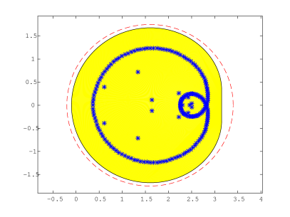
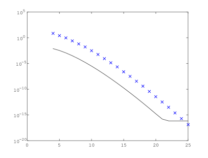
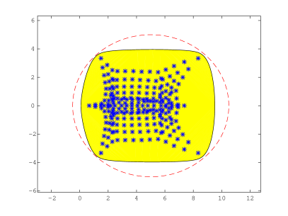
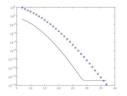
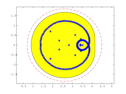
Figure 1 shows the behavior of the bound in (6) for the residual of the Arnoldi approximation of $e^{-A}\mathbf{v}$ with $\mathbf{v}=(1,\dots,1)^{T}/\sqrt{n}$. The top plots refer to $A\in{\cal B}_{200}(1,2)$ with Toeplitz structure, $A=\textrm{Toeplitz}(-1,1,\underline{2},0.1)$, where the underlined element is on the diagonal, while the previous (resp. subsequent) values denote the lower (resp. upper) diagonal entries. The bottom plots refer to the matrix pde225 of the Matrix Market repository matrixmarket . The left figure shows the field of values of the matrix $A$ (yellow area), its eigenvalues (“$\times$”), and the horizontal ellipse used in the bound (red dashed line). On the right we plot the residual associated with the Arnoldi approximation as the iteration proceeds (black solid line), and the corresponding values of the bound (blue crosses). Matrix exponentials were compute by the

xpm  Matlab function.
\

ndexm

In an inexact Arnoldi procedure $A$ is not known exactly. This may be due for instance to the fact that $A$ is only implicitly available via functional operations with a vector, which can be approximated at some accuracy. To proceed with our analysis we can formalize this inexactness at each iteration $k$ as

$$\widetilde{\mathbf{v}}_{k+1}=A{\mathbf{v}}_{k}+{\mathbf{w}}_{k}\approx A{\mathbf{v}}_{k}.$$ (7)

Typically, some form of accuracy criterion is implemented, so that $\|{\mathbf{w}}_{k}\|<\epsilon$ for some $\epsilon$. It may be that a different value of this tolerance is used at each iteration $k$, so that $\epsilon=\epsilon_{k}$. The new vector $\widetilde{\mathbf{v}}_{k+1}$ is then orthonormalized with respect to the previous basis vectors to obtain ${\mathbf{v}}_{k+1}$. In compact form, the original Arnoldi relation becomes

$$(A+{\cal E}_{m})V_{m}=V_{m}H_{m}+h_{m+1,m}\mathbf{v}_{m+1}\mathbf{e}_{m}^{T},\quad{\cal E}_{m}=[{\mathbf{w}}_{1},\ldots,{\mathbf{w}}_{m}]V_{m}^{*}.$$

Here $H_{m}$ is again upper Hessenberg; however, $H_{m}=V_{m}^{*}(A+{\cal E}_{m})V_{m}$. Moreover, ${\cal E}_{m}$ changes as $m$ grows. The differential equation residual can be defined in the same way as for the exact case, ${\mathbf{r}}_{m}=A{\mathbf{y}}_{m}-{\mathbf{y}}_{m}^{(d)}$; however the inexact Arnoldi relation should be considered to proceed further. Indeed,

$${\mathbf{r}}_{m} = A{\mathbf{y}}_{m}-{\mathbf{y}}_{m}^{(d)}=AV_{m}f(H_{m}){\mathbf{e}}_{1}-{\mathbf{y}}_{m}^{(d)}$$

$$= -{\cal E}_{m}V_{m}f(H_{m}){\mathbf{e}}_{1}+V_{m}H_{m}f(H_{m}){\mathbf{e}}_{1}-{\mathbf{y}}_{m}^{(d)}+{\mathbf{v}}_{m+1}h_{m+1,m}{\mathbf{e}}_{m}^{T}f(H_{m}){\mathbf{e}}_{1}$$

$$= -[{\mathbf{w}}_{1},\ldots,{\mathbf{w}}_{m}]f(H_{m}){\mathbf{e}}_{1}+{\mathbf{v}}_{m+1}h_{m+1,m}{\mathbf{e}}_{m}^{T}f(H_{m}){\mathbf{e}}_{1}.$$

Note that $\|{\mathbf{r}}_{m}\|$ is not available, since $A$ cannot be applied exactly. However, with the previous notation we can write $\|{\mathbf{r}}_{m}\|\leq|\|{\mathbf{r}}_{m}\|-r_{m}|+r_{m}$ where

$$|\|{\mathbf{r}}_{m}\|-r_{m}|\leq\|[{\mathbf{w}}_{1},\ldots,{\mathbf{w}}_{m}]f(H_{m}){\mathbf{e}}_{1}\|;$$

we remark that in this case $r_{m}\neq\|{\mathbf{r}}_{m}\|$. Therefore, checking the available $r_{m}$ provides a good measure of the accuracy in the function estimation as long as $\|[{\mathbf{w}}_{1},\ldots,{\mathbf{w}}_{m}]f(H_{m}){\mathbf{e}}_{1}\|$ is smaller than the requested tolerance for the final accuracy of the computation.

Clearly, $\|[{\mathbf{w}}_{1},\ldots,{\mathbf{w}}_{m}]f(H_{m}){\mathbf{e}}_{1}\|\leq\|[{\mathbf{w}}_{1},\ldots,{\mathbf{w}}_{m}]\|\,\|f(H_{m}){\mathbf{e}}_{1}\|$ so that the criterion $\|{\mathbf{w}}_{k}\|<\epsilon$ can be used to monitor the quality of the approximation to $f(A){\mathbf{v}}$ by means of $r_{m}$. However, a less stringent criterion can be devised. Following similar discussions in Simoncini.Szyld.03 ,Simoncini.05 , we write

$$\|[{\mathbf{w}}_{1},\ldots,{\mathbf{w}}_{m}]f(H_{m}){\mathbf{e}}_{1}\|=\|\sum_{j=1}^{m}{\mathbf{w}}_{j}{\mathbf{e}}_{j}^{T}f(H_{m}){\mathbf{e}}_{1}\|\leq\sum_{j=1}^{m}\|{\mathbf{w}}_{j}\|\,|{\mathbf{e}}_{j}^{T}f(H_{m}){\mathbf{e}}_{1}|,$$

where we assume that $\|{\mathbf{w}}_{j}\|<\epsilon_{j}$, that is the accuracy in the computation with $A$ varies with $j$. Hence, $\|[{\mathbf{w}}_{1},\ldots,{\mathbf{w}}_{m}]f(H_{m}){\mathbf{e}}_{1}\|$ is small when either $\|{\mathbf{w}}_{j}\|$ or $|{\mathbf{e}}_{j}^{T}f(H_{m}){\mathbf{e}}_{1}|$ is small, and not necessarily both. By exploiting the exponential decay of the entries of $f(H_{m}){\mathbf{e}}_{1}$, we can infer that $\|{\mathbf{w}}_{j}\|$ is in fact allowed to grow with $j$, according with the exponential decay of the corresponding entries of $f(H_{m}){\mathbf{e}}_{1}$, without affecting the overall accuracy. A priori bounds on $|{\mathbf{e}}_{j}^{T}f(H_{m}){\mathbf{e}}_{1}|$ can be used to select $\epsilon_{j}$ when estimating $A{\mathbf{v}}_{j}$. This relaxed strategy can significantly decrease the computational cost of matrix function evaluations whenever applying $A$ accurately is expensive. However, notice that the field of values of $H_{m}$ is contained in the field of values of $A+{\cal E}_{m}$. Hence if $W(A)$ is contained in an ellipse $\partial E$ of semi-axes $a,b$ and center $c$ then $W(A+{\cal E}_{m})\subset W(A)+W({\cal E}_{m})$. Since

$$\sup_{\|z\|=1}|z^{*}{\cal E}_{m}z|\leq\sup_{\|z\|=1}\|{\cal E}_{m}z\|\leq\sqrt{\sum_{j=1}^{m}\|{\mathbf{w}}_{j}\|^{2}}\leq\sqrt{\sum_{j=1}^{m}\epsilon_{j}^{2}}=:\epsilon^{(m)},$$

the set $W({\cal E}_{m})$ is contained in the disk centered at the origin and radius $\epsilon^{(m)}$. Therefore, $W(A)+W({\cal E}_{m})$ is contained in any set whose boundary has minimal distance from $\partial E$ not smaller than $\epsilon^{(m)}$. One such set is contained in the ellipse $\partial E_{m}$ with semi-axes $a(1+\epsilon^{(m)}/b)$, $b+\epsilon^{(m)}$ and center $c$. Indeed, $z\in\partial E_{m}$ can be parameterized as

$$z=\left(1+\frac{\epsilon^{(m)}}{b}\right)\frac{\rho}{2}\left(Re^{i\theta}+\frac{1}{Re^{i\theta}}\right)+c,\quad 0\leq\theta\leq 2\pi,$$

with $\rho=\sqrt{a^{2}-b^{2}}$, $R=(a+b)/\rho$. The distance between $z$ and the ellipse $\partial E$ is

$$\left|\frac{\epsilon^{(m)}}{b}\frac{\rho}{2}\left(Re^{i\theta}+\frac{1}{Re^{i\theta}}\right)\right|\geq\left|\frac{\epsilon^{(m)}}{b}\frac{\rho}{2}\left(R-\frac{1}{R}\right)\right|=\epsilon^{(m)}.$$

Hence we can provide the following strategy for the choice of the accuracy in inexact Arnoldi.

Theorem 3.2

Let ${\mathbf{r}}_{j}=A{\mathbf{y}}_{j}-{\mathbf{y}}_{j}^{(d)}$ be the residual obtained by the $j$th step of the inexact Arnoldi algorithm, with accuracy $\|w_{j}\|\leq\bar{\epsilon}_{j}$, for $j=1,2,\dots$. Consider an ellipse with semiaxes $a\geq b>0$ and center $c$ containing $W(A)$. Moreover, let us fix a tolerance $tol>0$, a maximum number of iterations $m$ and a value $\epsilon^{(m)}>0$. Then, the following choice for the accuracies

$$\bar{\epsilon}_{j}=\left\{\begin{array}[]{ll}\dfrac{tol}{m}\max\left(1,\dfrac{1}{s_{j}}\right),&\textrm{ if }\quad\dfrac{tol}{m\,s_{j}}<\dfrac{\sqrt{(\epsilon^{(m)})^{2}-\sum_{k=1}^{j-1}\bar{\epsilon}_{k}^{2}}}{m-j+1}\\ \\ \dfrac{\sqrt{(\epsilon^{(m)})^{2}-\sum_{k=1}^{j-1}\bar{\epsilon}_{k}^{2}}}{m-j+1},&\textrm{ otherwise }\end{array}\right.$$ (8)

for $j=1,\dots,m$, gives

$$\sqrt{\sum_{j=1}^{m}\bar{\epsilon}_{j}^{2}}\leq\epsilon^{(m)},\quad\textrm{ and }\quad|\|{\mathbf{r}}_{m}\|-r_{m}|\leq tol,$$

where $s_{j}$ is the upper bound for $|{\mathbf{e}}_{j}^{T}f(H_{m}){\mathbf{e}}_{1}|$ from Theorem 2.3 with $f$ the function associated with the solution of the differential equation $y^{(d)}=Ay$, and $E$ the ellipse with semiaxes $a(1+\epsilon^{(m)}/b)$, $b+\epsilon^{(m)}$ and center $c$. The bound can be specialized for the functions $f(z)=e^{z}$ and $f(z)=e^{-\sqrt{z}}$ using respectively corollaries 2.4 and 2.5.

Figure 2: Example 3.3, approximation of $e^{-A}\mathbf{v}$ with $\mathbf{v}=(1,\dots,1)^{T}/\sqrt{n}$. Residual norm $\|\mathbf{r}_{j}\|$ with constant accuracy $\epsilon_{j}=tol/m$, and residual norm $\|\mathbf{\bar{r}}_{j}\|$ with $\epsilon_{j}=\bar{\epsilon}_{j}$ by (8) as the inexact Arnoldi method proceeds. Left: For $A=\textrm{Toeplitz}(1,\underline{2},0.1,-1)\in{\cal B}_{200}(1,1)$. Right: For matrix pde225 from the Matrix Market repository matrixmarket .

Example 3.3

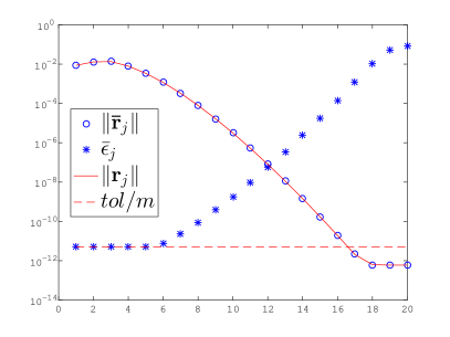
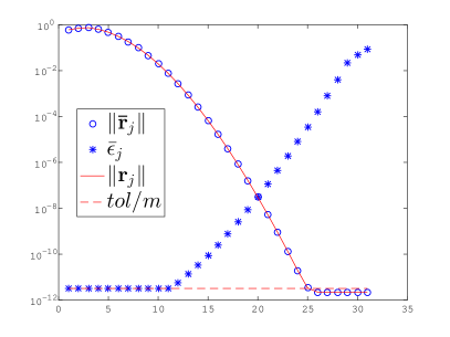
We consider the inexact Arnoldi procedure for the approximation of $\exp(-A)\mathbf{v}$, so that the norm of the differential equation residual is lower than a tolerance $tol$. The inexact matrix-vector product was implemented as in (7), where ${\bf w}_{j}$ is a random vector of norm $\epsilon_{j}$. Figure 2 reports our results for $\mathbf{v}=(1,\dots,1)^{T}/\sqrt{n}$ and the same matrices as in Example 3.1: $A=\textrm{Toeplitz}(1,\underline{2},0.1,-1)\in{\cal B}_{200}(2,1)$ (left), and the matrix pde225 from the Matrix Market repository matrixmarket (right). For constant accuracy $\epsilon_{j}=tol/m$ (dashed line), the solid line shows the residual norm $||\mathbf{r}_{j}||$ as the iteration $j$ proceeds. For variable accuracy $\epsilon_{j}=\bar{\epsilon}_{j}$ obtained from (8) (stars) the circles display the residual norm $\|\mathbf{\bar{r}}_{j}\|$. We set $tol=10^{-10}$ and $\epsilon^{(m)}=10^{-1}$. The maximum approximation space dimension $m$ was chosen as the smallest value for which the bound (6) is lower than $tol$, respectively $m=20$ and $m=31$. The fields of values of the matrices can be obtained starting from those reported in the left plots of Figure 1, where however now the original semi-axes $a,b$ of the elliptical sets considered for the computation of $s_{j}$ are increased by $\epsilon^{(m)}/b$ and $\epsilon^{(m)}$ respectively. The plots show visually overlapping residual norm histories for the two choices of $\epsilon_{j}$, illustrating that in practice no loss of information takes place during the relaxing strategy.

Figure 3: Example 3.4. Approximation of $e^{-A}\mathbf{v}$ with $A=\textrm{Toeplitz}(-1,1,\underline{3},0.1)\in\mathcal{B}_{200}(1,2)$ and $\mathbf{v}=(1,\dots,1)^{T}/\sqrt{n}$. Left: spectral information. Right: Residual norm $||\mathbf{r}_{j}||$ with constant accuracy $\epsilon_{j}=tol/m$, and residual norm $\|\mathbf{\bar{r}}_{j}\|$ with $\epsilon_{j}=\bar{\epsilon}_{j}$ by (8) as the inexact Arnoldi method proceeds.

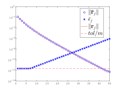
Consider the differential equation $y^{(2)}=Ay$, with $y(0)=\mathbf{v}$. Its solution can be expressed as $y(t)=\exp(-t\sqrt{A})\mathbf{v}$, and our results can be applied to this case as well. This time the upper bound $s_{j}$ for $|\mathbf{e}_{m}^{T}f(H_{m})\mathbf{e}_{1}|$ is obtained from Corollary 2.5.

Example 3.4

For the same experimental setting as in Example 3.3 we consider approximating $\exp(-\sqrt{A})\mathbf{v}$, for $A=\textrm{Toeplitz}(-1,1,\underline{3},0.1)\in\mathcal{B}_{200}(1,2)$, $\mathbf{v}=(1,\dots,1)^{T}/\sqrt{200}$ and $m=35$. Figure 3 reports on our findings, with the same description as for the previous example. Here $s_{j}$ in (8) is obtained from Corollary 2.5, and it is used to relax the accuracy $\epsilon_{j}$. Similar considerations apply.

4 Conclusions

Exploiting the described bounds for the off-diagonal decay pattern of functions of non-Hermitian banded matrices, we have derived bounds for the residual associated with the matrix function approximation given by the Arnoldi algorithm. As expected, the described bounds are influenced by the dependence between the predicted decay rate and the shape and dimension of the set enclosing the field of values of $A$. The closer $E$ is to the field of values, the sharper the bound. We have also used the described decay estimates to define a strategy for setting the accuracy of the inexactness of matrix-vector products in Arnoldi approximations of matrix functions applied to a vector. Similar results can be obtained for other Krylov-type approximations whose projection and restriction matrix $H_{m}$ has a semi-banded structure. This is the case for instance of the Extended Krylov subspace approximation; see, e.g., KnizhnermanSimoncini2010 and references therein.

Appendix A Technical proofs

Proof of corollary 2.4

Let $\rho=\sqrt{a^{2}-b^{2}}$ be the distance between the foci and the center of the ellipse (i.e., the boundary of $E$), and let $R=(a+b)/\rho$. Then a conformal map for $E$ is

$$\phi(w)=\frac{w-c-\sqrt{(w-c)^{2}-\rho^{2}}}{\rho R},$$ (9)

and its inverse is

$$\psi(z)=\frac{\rho}{2}\left(Rz+\frac{1}{Rz}\right)+c,$$ (10)

see, e.g., (suetin, , chapter II, Example 3). Notice that

$$\max_{|z|=\tau}|e^{\psi(z)}|=\max_{|z|=\tau}e^{\Re(\psi(z))}=e^{\frac{\rho}{2}\left(R\tau+\frac{1}{R\tau}\right)+c_{1}}.$$

Hence by Theorem 2.3 we get

$$\left|\left(e^{A}\right)_{k,\ell}\right|\leq 2\frac{\tau}{\tau-1}e^{c_{1}}e^{\frac{\rho}{2}\left(R\tau+\frac{1}{R\tau}\right)}\left(\frac{1}{\tau}\right)^{\xi}.$$

The optimal value of $\tau>1$ that minimizes $e^{\frac{\rho}{2}\left(R\tau+\frac{1}{R\tau}\right)}\left(\frac{1}{\tau}\right)^{\xi}$ is

$$\tau=\frac{\xi+\sqrt{\xi^{2}+\rho^{2}}}{\rho R}.$$

Moreover the condition $\tau>1$ is satisfied if and only if $\xi>\frac{\rho}{2}\left(R-\frac{1}{R}\right)=b$. Finally, noticing that

$$\psi\left(\frac{\xi+\sqrt{\xi^{2}+\rho^{2}}}{\rho R}\right)-c_{1}=\frac{1}{2}\left(\xi+\sqrt{\xi^{2}+\rho^{2}}+\frac{\rho^{2}}{\xi+\sqrt{\xi^{2}+\rho^{2}}}\right)=\xi q(\xi),$$

and collecting $\xi$ the proof is completed. ∎

Proof of corollary 2.5

The function $f(z)=\exp(-\sqrt{z})$ is analytic on $\mathbb{C}\setminus(-\infty,0)$. Since we consider the principal square root, then $\Re(\sqrt{z})\geq 0$, and so

$$|\exp(-\sqrt{z})|=\exp(-\Re(\sqrt{z}))\leq 1.$$

Hence, by Theorem 2.3 we can determine $\tau$ for which

$$\left|\left(e^{-\sqrt{A}}\right)_{k,\ell}\right|\leq 2\frac{\tau}{\tau-1}\left(\frac{1}{\tau}\right)^{\xi}.$$

For every $\varepsilon>0$ close enough to zero, we set the parameter

$$\tau_{\varepsilon}=|\phi(\varepsilon)|=\left|\frac{c-\varepsilon+\sqrt{(c-\varepsilon)^{2}-\rho^{2}}}{\rho R}\right|,$$

with $\phi(w)$ as in (9) and $\psi(z)$ its inverse (10). Then the ellipse $\{\psi(z),\,|z|=\tau_{\varepsilon}\}$ is contained in $\mathbb{C}\setminus(-\infty,0]$. Letting $\varepsilon\rightarrow 0$ concludes the proof. ∎

References

- (1) Afanasjew, M., Eiermann, M., Ernst, O.G., Güttel, S.: Implementation of a restarted Krylov subspace method for the evaluation of matrix functions. Linear Algebra Appl. 429(10), 2293–2314 (2008). DOI 10.1016/j.laa.2008.06.029. URL https://doi.org/10.1016/j.laa.2008.06.029
- (2) Beckermann, B.: Image numérique, GMRES et polynômes de Faber. C. R. Math. Acad. Sci. Paris 340(11), 855–860 (2005)
- (3) Benzi, M., Boito, P.: Decay properties for functions of matrices over -algebras. Linear Algebra Appl. 456, 174–198 (2014). DOI 10.1016/j.laa.2013.11.027. URL http://dx.doi.org/10.1016/j.laa.2013.11.027
- (4) Benzi, M., Boito, P., Razouk, N.: Decay Properties of Spectral Projectors with Applications to Electronic Structure. SIAM Rev. 55(1), 3–64 (2013). DOI 10.1137/100814019. URL http://dx.doi.org/10.1137/100814019
- (5) Benzi, M., Golub, G.H.: Bounds for the Entries of Matrix Functions with Applications to Preconditioning. BIT 39(3), 417–438 (1999). DOI 10.1023/A:1022362401426. URL http://dx.doi.org/10.1023/A:1022362401426
- (6) Benzi, M., Razouk, N.: Decay bounds and O(n) algorithms for approximating functions of sparse matrices. Electron. Trans. Numer. Anal. 28, 16–39 (2007)
- (7) Benzi, M., Simoncini, V.: Decay bounds for functions of Hermitian matrices with banded or Kronecker structure. SIAM J. Matrix Anal. Appl. 36(3), 1263–1282 (2015). DOI 10.1137/151006159. URL http://dx.doi.org/10.1137/151006159
- (8) Botchev, M.A., Grimm, V., Hochbruck, M.: Residual, restarting and Richardson iteration for the matrix exponential. SIAM J. Sci. Comput. 35(3), A1376–A1397 (2013)
- (9) Canuto, C., Simoncini, V., Verani, M.: On the decay of the inverse of matrices that are sum of Kronecker products. Linear Algebra Appl. 452, 21–39 (2014). DOI 10.1016/j.laa.2014.03.029. URL http://dx.doi.org/10.1016/j.laa.2014.03.029
- (10) Cowen, C.C., Harel, E.: An Effective Algorithm for Computing the Numerical Range (1995). Https://www.math.iupui.edu/ ccowen/Downloads/33NumRange.html
- (11) Del Buono, N., Lopez, L., Peluso, R.: Computation of the exponential of large sparse skew-symmetric matrices. SIAM J. Sci. Comput. 27(1), 278–293 (2005). DOI 10.1137/030600758. URL http://dx.doi.org/10.1137/030600758
- (12) Demko, S.G.: Inverses of band matrices and local convergence of spline projections. SIAM J. Numer. Anal. 14(4), 616–619 (1977). DOI 10.1137/0714041. URL http://dx.doi.org/10.1137/0714041
- (13) Demko, S.G., Moss, W.F., Smith, P.W.: Decay rates for inverses of band matrices. Math. Comp. 43(168), 491–499 (1984). DOI 10.2307/2008290. URL http://dx.doi.org/10.2307/2008290
- (14) Dinh, K.N., Sidje, R.B.: Analysis of inexact Krylov subspace methods for approximating the matrix exponential. Math. Comput. Simul. 138, 1–13 (2017). DOI 10.1016/j.matcom.2017.01.002. URL http://www.sciencedirect.com/science/article/pii/S0378475417300034
- (15) Druskin, V., Knizhnerman, L.: Krylov subspace approximation of eigenpairs and matrix functions in exact and computer arithmetic. Numer. Linear Algebra Appl. 2(3), 205–217 (1995). DOI 10.1002/nla.1680020303. URL http://dx.doi.org/10.1002/nla.1680020303
- (16) Eiermann, M.: Fields of values and iterative methods. Linear Algebra Appl. 180, 167–197 (1993). DOI 10.1016/0024-3795(93)90530-2. URL http://dx.doi.org/10.1016/0024-3795(93)90530-2
- (17) Eiermann, M., Ernst, O.G., Güttel, S.: Deflated restarting for matrix functions. SIAM J. Matrix Anal. Appl. 32(2), 621–641 (2011)
- (18) Eijkhout, V., Polman, B.: Decay rates of inverses of banded M-matrices that are near to Toeplitz matrices. Linear Algebra Appl. 109, 247–277 (1988). DOI 10.1016/0024-3795(88)90211-X. URL http://www.sciencedirect.com/science/article/pii/002437958890211X
- (19) Ellacott, S.W.: Computation of Faber series with application to numerical polynomial approximation in the complex plane. Math. Comp. 40(162), 575–587 (1983)
- (20) Freund, R.: On polynomial approximations to with complex and some applications to certain non-hermitian matrices. Approx. Theory Appl. 5, 15–31 (1989)
- (21) Frommer, A., Güttel, S., Schweitzer, M.: Convergence of restarted Krylov subspace methods for Stieltjes functions of matrices. SIAM J. Matrix Anal. Appl. 35(4), 1602–1624 (2014)
- (22) Frommer, A., Güttel, S., Schweitzer, M.: Efficient and stable Arnoldi restarts for matrix functions based on quadrature. SIAM J. Matrix Anal. Appl. 35(2), 661–683 (2014). DOI 10.1137/13093491X. URL https://doi.org/10.1137/13093491X
- (23) Frommer, A., Schimmel, C., Schweitzer, M.: Bounds for the decay of the entries in inverses and Cauchy–Stieltjes functions of certain sparse, normal matrices. Numer. Linear Algebra Appl. 25(4), e2131 (2018). DOI 10.1002/nla.2131
- (24) Güttel, S.: Rational Krylov approximation of matrix functions: numerical methods and optimal pole selection. GAMM-Mitt. 36(1), 8–31 (2013). DOI 10.1002/gamm.201310002. URL http://dx.doi.org/10.1002/gamm.201310002
- (25) Güttel, S., Knizhnerman, L.: A black-box rational Arnoldi variant for Cauchy-Stieltjes matrix functions. BIT 53(3), 595–616 (2013). DOI 10.1007/s10543-013-0420-x. URL https://doi.org/10.1007/s10543-013-0420-x
- (26) Higham, N.J.: Functions of Matrices: Theory and Computation. Society for Industrial and Applied Mathematics, Philadelphia, PA, USA (2008)
- (27) Hochbruck, M., Lubich, C.: On Krylov subspace approximations to the matrix exponential operator. SIAM J. Numer. Anal. 34, 1911–1925 (1997)
- (28) Iserles, A.: How large is the exponential of a banded matrix? New Zealand J. Math. 29, 177–192 (2000)
- (29) Knizhnerman, L., Simoncini, V.: A new investigation of the extended Krylov subspace method for matrix function evaluations. Numer. Linear Algebra Appl. 17(4), 615–638 (2010). DOI 10.1002/nla.652. URL http://dx.doi.org/10.1002/nla.652
- (30) Kürschner, P., Freitag, M.A.: Inexact methods for the low rank solution to large scale Lyapunov equations. arXiv preprint arXiv:1809.06903 (2018)
- (31) Matrix Market: A Visual Repository of Test Data for Use in Comparative Studies of Algorithms for Numerical Linear Algebra. Mathematical and Computational Sciences Division, National Institute of Standards and Technology; available online at http://math.nist.gov/ MatrixMarket
- (32) Mastronardi, N., Ng, M., Tyrtyshnikov, E.E.: Decay in functions of multiband matrices. SIAM J. Matrix Anal. Appl. 31(5), 2721–2737 (2010). DOI 10.1137/090758374. URL http://dx.doi.org/10.1137/090758374
- (33) The MathWorks, Inc.: MATLAB 7, r2013b edn. (2013)
- (34) Meurant, G.: A review on the inverse of symmetric tridiagonal and block tridiagonal matrices. SIAM J. Matrix Anal. Appl. 13(3), 707–728 (1992). DOI 10.1137/0613045. URL http://dx.doi.org/10.1137/0613045
- (35) Pozza, S., Tudisco, F.: On the stability of network indices defined by means of matrix functions. SIAM J. Matrix Anal. Appl. 39(4), 1521–1546 (2018)
- (36) Rinehart, R.F.: The equivalence of definitions of a matric function. Amer. Math. Monthly 62(6), 395–414 (1955)
- (37) Saad, Y.: Analysis of some Krylov subspace approximations to the matrix exponential operator. SIAM J. Numer. Anal. 29(1), 209–228 (1992). URL http://epubs.siam.org/doi/abs/10.1137/0729014
- (38) Simoncini, V.: Variable accuracy of matrix-vector products in projection methods for eigencomputation. SIAM J. Numer. Anal. 43(3), 1155–1174. (2005)
- (39) Simoncini, V., Szyld, D.B.: Theory of inexact Krylov subspace methods and applications to scientific computing. SIAM J. Sci. Comput. 25(2), 454–477 (2003)
- (40) Suetin, P.K.: Series of Faber polynomials. Gordon and Breach Science Publishers (1998). Translated from the 1984 Russian original by E. V. Pankratiev [E. V. Pankrat′ev]
- (41) Wang, H.: The Krylov Subspace Methods for the Computation of Matrix Exponentials. Ph.D. thesis, Department of Mathematics, University of Kentucky (2015)
- (42) Wang, H., Ye, Q.: Error bounds for the Krylov subspace methods for computations of matrix exponentials. SIAM J. Matrix Anal. Appl. 38(1), 155–187 (2017). URL https://doi.org/10.1137/16M1063733
- (43) Ye, Q.: Error bounds for the Lanczos methods for approximating matrix exponentials. SIAM J. Numer. Anal. 51(1), 68–87 (2013). DOI 10.1137/11085935x. URL http://dx.doi.org/10.1137/11085935X