Domain wall theory and non-stationarity in driven flow with exclusion

Abstract

We study the dynamical evolution toward steady state of the stochastic non-equilibrium model known as totally asymmetric simple exclusion process, in both uniform and non-uniform (staggered) one-dimensional systems with open boundaries. Domain-wall theory and numerical simulations are used and, where pertinent, their results are compared to existing mean-field predictions and exact solutions where available. For uniform chains we find that the inclusion of fluctuations inherent to the domain-wall formulation plays a crucial role in providing good agreement with simulations, which is severely lacking in the corresponding mean-field predictions. For alternating-bond chains the domain-wall predictions for the features of the phase diagram in the parameter space of injection and ejection rates turn out to be realized only in an incipient and quantitatively approximate way. Nevertheless, significant quantitative agreement can be found between several additional domain-wall theory predictions and numerics.

I Introduction

In this paper we consider the dynamic evolution of the totally asymmetric simple exclusion process (TASEP) in both uniform and non-uniform one-dimensional (1D) systems. The TASEP, in its original version for uniform chains, already exhibits many non-trivial properties including flow phase changes, because of its collective character derr98 ; sch00 ; mukamel ; derr93 ; rbs01 ; be07 ; cmz11 , and is considered paradigmatic of non-equilibrium statistical mechanical models. We make use of the domain-wall (DW) approach ksks98 ; ps99 ; ds00 ; sa02 , coupled with numerical simulations.

Application of mean-field (MF) Mobius mapping hex13 ; hex15 to generalizations of the TASEP such as non-uniform chains and hexagonal-lattice systems turns out to provide less accurate steady state results than for the well-known uniform 1D case. And for dynamics hex15 , some significant discrepancies between MF predictions and numerics already arise for uniform 1D systems. Such inadequacies motivate the formulation of a DW theory (which includes fluctuations altogether absent in MF) to provide further understanding of the physical processes underlying this model.

In Sec. II we review the DW theory for uniform chains, and develop a generalization which applies for 1D systems with alternating bond rates. In Sec. III we give results of the numerically calculated DW evolution predicted by theory, as well as those from direct simulations of the stochastic TASEP process. In Section IV, we summarize and discuss our results.

II Theory

II.1 Uniform chain

We here briefly review basic aspects of the TASEP, and of its DW representation, for the simplest case, uniform chains derr98 ; sch00 ; mukamel ; derr93 ; rbs01 ; be07 ; cmz11 ; ksks98 ; ps99 ; ds00 ; sa02 .

In the TASEP the particle number $n_{\ell}$ at lattice site $\ell$ can be $0$ or $1$. Any such "exclusion" configuration of particles (having at most one particle at any site) can evolve by hopping of the particle at any occupied site $\ell$ to the adjacent site $\ell+1$, provided it is empty. The instantaneous current $J_{\ell\,\ell+1}$ across the bond from $\ell$ to $\ell+1$ depends also on the stochastic attempt rate, or bond (transmissivity) rate, $p_{\ell}$, associated with it. In the uniform TASEP, $p_{\ell}=p$ for all “internal bonds” $\ell$ (i.e. other than the injection and ejection ones for the open-chain case, see below). Thus,

$$J_{\ell\,\ell+1}=\begin{cases}{n_{\ell}(1-n_{\ell+1})\quad{\rm with\ probability}\ p_{\ell}}\cr{0\qquad\qquad\qquad{\rm with\ probability}\ 1-p_{\ell}\ .}\end{cases}$$ (1)

The "open" chain with additional processes (subject to the exclusion constraint) of injection at rate $\alpha$ at the left boundary, and ejection at rate $\beta$ at the right boundary is of particular interest, because of its rich behavior, including boundary-driven phase transitions and associated static and dynamic critical behavior. Its properties, particularly densities, currents, and associated correlation functions, will be studied in what follows.

One such property is the density profile $\rho(\ell,t)$ given by the average of occupations at site $\ell$ and time $t$, over all possible realizations of the evolution up to time $t$. In general such quantities evolve in time towards an eventual steady-state form which, for the open chain, depends on the boundary conditions through $\alpha$, $\beta$, but not on initial conditions.

The simplest approach, MF theory mukamel ; rbs01 , already distinguishes the different phases, through current and density averages and especially through the forms of the density profile. Remarkably MF theory gives the phase boundaries in the ($\alpha,\beta$) plane exactly for the uniform chain mukamel ; rbs01 .

A particular example of an MF steady state density profile is that for $\alpha=\beta<1/2$, corresponding to the coexistence line in the low current phase. This profile, for large system size, provides a ’macroscopic’ view of the system state, in which a narrow domain wall separates a domain on the left side, with uniform site occupation (local density) $\rho^{-}$ controlled by the injection rate from another on the right with uniform site occupation $\rho^{+}$:

$$\rho^{-}=\alpha\quad;\qquad\rho^{+}=1-\beta\ ;$$ (2)

and similarly for the mean field currents in the two domains.

However these steady state currents do not balance at the domain wall, if it is stationary. This and other examples at different ($\alpha,\beta$) indicates the need to allow for (stochastic) motion of the domain wall. This is the motivation for the DW theory, which can restore the particle conservation and include fluctuations absent from mean field theory ksks98 ; ps99 ; ds00 ; sa02 .

One postulates that the TASEP process can be represented by the stochastic hopping of the domain wall. For simplicity we make all bond rates $p_{\ell}\equiv 1$, see Eq. 1.

To be consistent with the particle currents near the wall one has to allow for possibly asymmetric hopping rates $D^{+}$, $D^{-}$ given by:

$$D^{-}=\frac{j^{-}}{\Delta\rho}=\frac{\alpha(1-\alpha)}{1-\alpha-\beta}\ ;$$

$$D^{+}=\frac{j^{+}}{\Delta\rho}=\frac{\beta(1-\beta)}{1-\alpha-\beta}\ .$$ (3)

Here $\Delta\rho\equiv\rho^{+}-\rho^{-}=1-\alpha-\beta$, and the currents $j^{+}$, $j^{-}$ within each domain are assumed ksks98 to take the MF (i.e., factorized) form

$$j^{-}=\rho^{-}(1-\rho^{-})=\alpha(1-\alpha)\ ;$$

$$j^{+}=\rho^{+}(1-\rho^{+})=\beta(1-\beta)\ .$$ (4)

Despite the simplicity of the approach it does include fluctuations absent from the MF picture and in some cases vastly improves on the MF description, e.g., in giving certain exact results for the uniform chain (see, e.g., Sec. III).

For a chain with $N$ sites and $L\equiv N+1$ bonds (including the injection and ejection ones), the time evolution of the probability $P(\ell,t)$ of finding the domain wall at "bond $\ell$" (meaning the bond joining sites $\ell$ and $\ell+1$) for time $t$ is given by:

$$\frac{dP(\ell,t)}{dt}=D^{+}P(\ell-1,t)+D^{-}P(\ell+1,t)-$$

$$-\left(D^{+}+D^{-}\right)P(\ell,t)\ ,$$ (5)

for internal bonds $1\leq\ell\leq N-1$. At the boundaries one has:

$$\frac{P(0,t)}{dt}=D^{-}P(1,t)-D^{+}P(0,t)\ ;$$ (6)

$$\frac{dP(L,t)}{dt}=D^{+}P(L-1,t)-D^{-}P(L,t)\ .\quad\$$ (7)

The general solution to Eqs. (5)–(7) can be found by assuming a linear superposition of forms $u^{\ell}\,e^{R(u)t}$. Direct substitution into Eq. (5) shows that the following relation holds:

$$R(u)=\left(D^{-}-\frac{D^{+}}{u}\right)(u-1)\ .$$ (8)

So the steady-state solution $P_{s}(\ell)$, i.e. having $u$ such that $R(u)=0$, is

$$P_{s}(\ell)=c_{1}\,\left(\frac{D^{+}}{D^{-}}\right)^{\ell}+c_{2}\ ,$$ (9)

thus (for $D^{+}/D^{-}\neq 1$), the steady state density profile involves the exponential factor $e^{\lambda_{s}\ell}$ where

$$\lambda_{s}=\ln\left(\frac{D^{+}}{D^{-}}\right)\ ,$$ (10)

corresponding to the wall being spread over a distance $\sim 1/|\lambda_{s}|$ at one side of the system. The time-dependent part of the full solution is formed by grouping together the degenerate factorizable solutions with $u$ and ${\bar{u}}=D^{+}/(D^{-}u)$ [ such that $R({\bar{u}})=R(u)\,$] into forms:

$$f(u,t)=\left[A\,u^{\ell}+B\left(\frac{D^{+}}{D^{-}}\frac{1}{u}\right)^{\ell}\,\right]e^{R(u)t}\ .$$ (11)

The boundary conditions given in Eqs. (6) and (7) determine the allowed (discretized) $u$’s ($\equiv u_{n}$) and the ratio of the coefficients $A$, $B$. So,

$$P(\ell,t)=\sum_{n}\left(A_{n}\,u_{n}^{\ell}+B_{n}\,{\bar{u}_{n}}^{\ell}\right)\,e^{R(u_{n})t}+P_{s}(\ell)\ ,$$ (12)

where

$$u_{n}=e^{\lambda_{d}}\,e^{iq_{n}}\ ;\quad{\bar{u}_{n}}=u_{n}^{\ast}\ ,$$ (13)

and

$$\frac{B_{n}}{A_{n}}=-\frac{(e^{\lambda_{d}}-e^{iq_{n}})}{(e^{\lambda_{d}}-e^{-iq_{n}})}\ ,$$ (14)

with

$$\lambda_{d}=\ln\sqrt{\frac{D^{+}}{D^{-}}}=\frac{1}{2}\lambda_{s}\ ;\quad q_{n}=\frac{n\pi}{L}\ ,$$ (15)

and

$$R(u_{n})=D^{+}+D^{-}-2\left[D^{+}D^{-}\right]^{1/2}\cos\frac{n\pi}{L}\equiv R_{n}\ .$$ (16)

Once the probability $P(\ell,t)$ has been obtained, the density profile is given from:

$$\rho(\ell+1,t)-\rho(\ell,t)=\Delta\rho\,P(\ell,t)\ .$$ (17)

.

II.2 Staggered chain

We next apply a DW approach to the TASEP with alternating bond rates. The geometry requires a generalization of the usual macroscopic view, leading to new relationships of microscopic currents and densities to quantities such as diffusion rates. Of course macroscopic views apply to each sublattice separately, but their interpenetration requires detailed consideration of the particle current between sites on opposite sublattices. As usual in DW theory these currents are those in the MF steady state, which are the same on all bonds (of either sublattice) in a given domain. As in uniform chains with a domain wall, there remains the distinction between the uniform, MF steady state, densities $\rho^{+}$ and $\rho^{-}$ in domains on either side of the wall. But now these densities also differ between the two sublattices, which we distinguish by subscripts $1$ or $2$. The generalized hopping picture and the labeling on bonds of hopping rates ($p_{1}$,$p_{2}$) and currents ($J_{12}^{\pm}$,$J_{21}^{\pm}$), and of particle densities ($\rho_{1}^{\pm}$,$\rho_{2}^{\pm}$) at sites, are shown in Fig. 1.

Figure 1: A domain wall (dashed vertical line) dividing a two-sublattice system with alternating hopping rates $p_{1}$, $p_{2}$, into a ’minus’ domain (left) and a ’plus’ one (see text for definitions of $\rho^{\pm}_{1,2}$ and $J^{\pm}_{12,21}$).

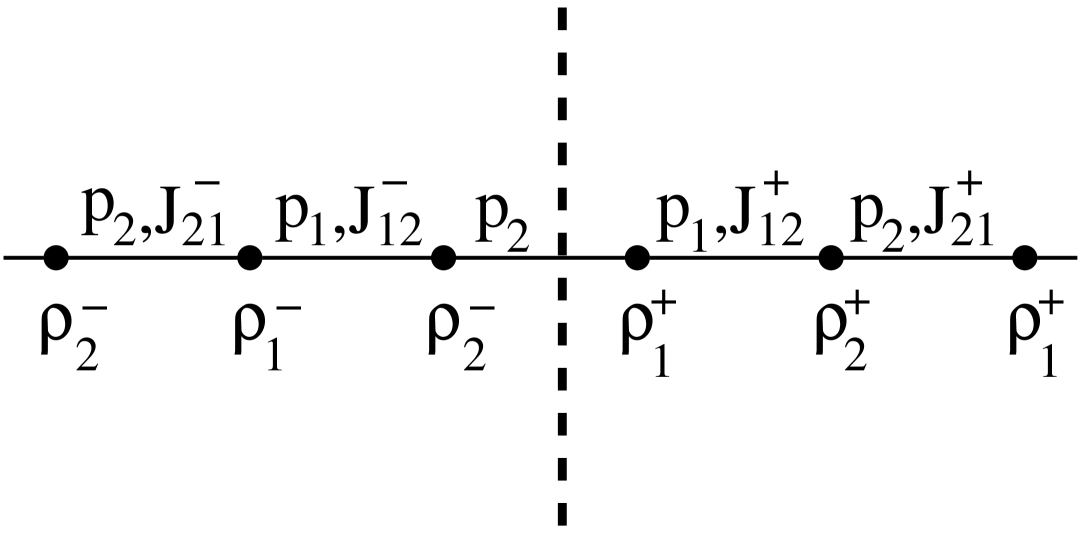
The DW diffusion constants, resulting from particle conservation, for hopping to right or left ($+$ or $-$) from a given type of bond ($1$ or $2$) are given by

$$D^{-}_{2}\left(\rho^{+}_{2}-\rho^{-}_{2}\right)=J^{-}_{12}\equiv p_{1}\,\rho^{-}_{1}\left(1-\rho^{-}_{2}\right)\ ;$$ (18)

$$D^{+}_{1}\left(\rho^{+}_{1}-\rho^{-}_{1}\right)=J^{+}_{12}\equiv p_{1}\,\rho^{+}_{1}\left(1-\rho^{+}_{2}\right)\ ;$$ (19)

$$D^{+}_{2}\left(\rho^{+}_{2}-\rho^{-}_{2}\right)=J^{+}_{21}\equiv p_{2}\,\rho^{+}_{2}\left(1-\rho^{+}_{1}\right)\ ;$$ (20)

$$D^{-}_{1}\left(\rho^{+}_{1}-\rho^{-}_{1}\right)=J^{-}_{21}\equiv p_{2}\,\rho^{-}_{2}\left(1-\rho^{-}_{1}\right)\ .$$ (21)

Eq. (18), for example, follows from the hopping picture and the labeling of bond rates and currents and site densities shown in Fig. 1 because in the left hop of the wall shown, the bond left of the wall, with current $J_{12}^{-}$, carries $\rho^{+}_{2}-\rho^{-}_{2}$ across to the right.

As for the uniform chain, the application of DW diffusion theory to the staggered chain needs the identification of incipient walls, typically from MF steady state density profiles, and their characterization. That involves finding hopping rates, using Eqs. (18)–(21) with appropriate currents and densities. These can come from Mobius maps hex13 ; hex15 involving the parameters $\alpha$, $\beta$, $p_{1}$, $p_{2}$.

A variety of different forms arise, corresponding to the different regions of the MF steady state phase diagram. The MF phase boundaries, as well as coexistence and possible factorization lines, turn out to be only approximate for the staggered chain hex15 , and they can be shifted by fluctuations. Their possible modification by DW diffusion is of particular interest and we first address that.

For the staggered chain there is no known analogue of the operator algebra which holds for the uniform case, and from which the existence of factorizable states can be established, so here our use of the term "factorization" should be taken to cover the possibility of factorization through a state of uniform density. This issue will be discussed conclusively in Sec. IV.

The DW diffusion steady state density profiles (on each sublattice) which determine such things are related to the steady state diffusion probability distribution $P_{\ell}$ for each sublattice, through a generalization of Eq. (9). As in the uniform chain, these $P_{\ell}$’s typically include parts exponential in $\ell$. The (coupled) steady state diffusion equations result in

$$P_{\ell}=c_{1}\,\left(\frac{D^{+}_{1}D^{+}_{2}}{D^{-}_{1}D^{-}_{2}}\right)^{\ell/2}+c_{2}\ \qquad{\rm(steady\ state)}\ ,$$ (22)

with different constants for the two sublattices.

In the phase diagram the coexistence and factorization lines are special in having site-independent $P_{\ell}$’s. This can only occur if

$$\frac{D^{+}_{1}D^{+}_{2}}{D^{-}_{1}D^{-}_{2}}=1\ ,$$ (23)

analogous to having overall zero bias.

For converting the condition Eq. (23) to a relation between $\alpha$, $\beta$, $p_{1}$, $p_{2}$, one needs the MF steady state densities (uniform on each domain) for both sublattices, namely $\rho^{-}_{1}$, $\rho^{-}_{2}$, $\rho^{+}_{1}$, $\rho^{+}_{2}$. With the injection and ejection sites both on sublattice $1$,

$$\rho^{-}_{1}=\frac{ap_{2}}{p_{1}+a(p_{2}-p_{1})}\ ,\ \ 1-\rho^{+}_{1}=\frac{bp_{1}}{p_{2}+b(p_{1}-p_{2})}\ ;$$ (24)

$$\rho^{-}_{2}=a\ ,\qquad\quad\qquad\qquad 1-\rho^{+}_{2}=b\ ,\qquad$$ (25)

where $a=\alpha/p_{2}$, $b=\beta/p_{1}$.

With $A\equiv p_{1}+a(p_{2}-p_{1})$, $B\equiv p_{2}+b(p_{1}-p_{2})$, $C\equiv 1-a-b$, we find for the diffusion rates:

$$D^{+}_{1}=b(1-b)\,\frac{A}{C}\;$$

$$D^{+}_{2}=p_{1}p_{2}\,\frac{b(1-b)}{BC}\ ;$$

$$D^{-}_{2}=p_{1}p_{2}\,\frac{a(1-a)}{AC}\ ;$$

$$D^{-}_{1}=a(1-a)\,\frac{B}{C}\ .$$ (26)

The sublattice density differences are

$$\rho^{+}_{2}-\rho^{-}_{2}=C\ ;\qquad\rho^{+}_{1}-\rho^{-}_{1}=p_{1}p_{2}\,\frac{C}{AB}\ ,$$ (27)

and we have

$$\frac{D^{+}_{1}D^{+}_{2}}{D^{-}_{1}D^{-}_{2}}=\left[\frac{b(1-b)A}{a(1-a)B}\right]^{2}\ .$$ (28)

This last result makes the condition Eq. (23) for the coexistence and factorization lines, in DW theory, become

$$b(1-b)\left[p_{1}+a(p_{2}-p_{1})\right]=\pm a(1-a)\left[p_{2}+b(p_{1}-p_{2})\right]\ ,$$ (29)

giving, respectively:

$$p_{1}\,\left(\frac{1-a}{a}\right)=p_{2}\,\left(\frac{1-b}{b}\right)\quad{\rm(coexistence)}\ ;\\$$ (30)

$$a+b=1\qquad{\rm(factorization)}\ .$$ (31)

It turns out that these determining equations are the same as in MF theory [ where they come from the steady state equivalence of bond currents, with the uniform density profiles given by Eqs. (24), (25) ].

The rather general relations just given for diffusion rates and associated quantities can need reinterpretation, e.g., to avoid sign errors in $D$’s, for certain regions of the phase diagram.

The intersection of the factorization and coexistence lines is the critical point

$$(a_{c},b_{c})=\left(\frac{\sqrt{p_{1}}}{\sqrt{p_{1}}+\sqrt{p_{2}}},\frac{\sqrt{p_{2}}}{\sqrt{p_{1}}+\sqrt{p_{2}}}\right)\ ,$$ (32)

predicted by both MF and DW theory.

We next turn to dynamical behavior within DW theory, which needs use of the full coupled discrete diffusion equations for the domain wall. Omitting the time dependence for clarity, and recalling that odd- and even-numbered lattice sites correspond respectively to sublattices $1$ and $2$, these are:

$$\frac{dP_{2\ell}}{dt}=P_{2\ell-1}D^{+}_{2}+P_{2\ell+1}D^{-}_{1}-(D^{+}_{2}+D^{-}_{1})P_{2\ell}\ ;$$ (33)

$$\frac{dP_{2\ell+1}}{dt}=P_{2\ell}D^{+}_{1}+P_{2\ell+2}D^{-}_{2}-(D^{+}_{1}+D^{-}_{2})P_{2\ell+1}\ .$$ (34)

The solution of Eqs. (33)–(34) involves the following two (sublattice) superpositions of factorizable components

$$P_{2\ell}=\sum_{\zeta}A_{\zeta}\,e^{2\ell\zeta}\,e^{-tR(\zeta)}\ ;$$ (35)

$$P_{2\ell+1}=\sum_{\zeta}B_{\zeta}\,e^{(2\ell+1)\zeta}\,e^{-tR(\zeta)}\ .$$ (36)

The resulting equations for $R(\zeta)$ and $B_{\zeta}/A_{\zeta}$ involve the matrix

$${\cal M}=\begin{pmatrix}{a(0)}&-a(\zeta)\cr{-b(\zeta)}&{b(0)}\end{pmatrix}\ {\rm with}\ \begin{cases}{a(\zeta)=D^{+}_{2}e^{-\zeta}+D^{-}_{1}e^{\zeta}}\cr{b(\zeta)=D^{+}_{1}e^{-\zeta}+D^{-}_{2}e^{\zeta}\ .}\end{cases}$$ (37)

The eigenvalues and eigenvectors of $\cal M$ provide a two-branch spectrum for $R(\zeta)$, and corresponding values of the ratio $B_{\zeta}/A_{\zeta}$.

A few general remarks can be made here. One is that specifying $R(\zeta)=0$ requires that the determinant of $\cal M$ should vanish, which is satisfied if $\zeta={\bar{\zeta}}$ where

$$e^{2{\bar{\zeta}}}=\frac{D^{+}_{1}D^{+}_{2}}{D^{-}_{1}D^{-}_{2}}\ .$$ (38)

This is the "complex wave vector" corresponding to the exponential profiles in steady state, see Eq. (22).

Another remark concerns boundary conditions. These require that the differences of the profiles from their steady state values have to vanish at the boundaries; and they determine the allowed $\zeta$’s.

As in the uniform chain [ see Eq. (11) ] the boundary requirements can be satisfied by grouping degenerate factorizable solutions, having $\zeta$’s with the same $R(\zeta)$. The eigenvalue equation for $R(\zeta)$ is

$$R^{2}-\Sigma\,R+G(\zeta)=0\ ,$$ (39)

where

$$\Sigma=D^{+}_{1}+D^{+}_{2}+D^{-}_{1}+D^{-}_{2}$$ (40)

and, with

$$\Gamma=\sqrt{D^{+}_{1}D^{+}_{2}D^{-}_{1}D^{-}_{2}}\ ,$$ (41)

$$G(\zeta)=2\Gamma\,\left(\cosh{\bar{\zeta}}-\cosh(2\zeta-{\bar{\zeta}})\right)\ .$$ (42)

So, degenerate $\zeta$’s all have the same $G$, and a particular such group is easily seen to be $z$, ${\bar{\zeta}}-z$, $z-\pi\,i$, ${\bar{\zeta}}+\pi\,i-z$, e.g. with $z$ real.

The generalization obtained by adding $\pm i\,q$ to each of these provides a group all with the same ${\rm Re}\ R$’s and equal or opposite ${\rm Im}\ R$’s (proportional to ballistic velocities). Superpositions involving such a group provide the time-dependent parts of solutions which can satisfy the boundary conditions. The remaining requirements are

$$z=\frac{\bar{\zeta}}{2}\ ;\qquad q=q_{n}=\frac{n\pi}{L}\ ,$$ (43)

together with conditions relating the coefficients $A_{\zeta}$, $B_{\zeta}$ for all the $\zeta$’s of the group. Initial conditions complete the determination of the coefficients.

The above procedure for dealing with the boundary conditions for the staggered chain is much more complicated than that in Sec. II.1, but the result Eq. (43) is of the same form as Eq. (15).

So the rate $R$ is provided by inserting $G(\frac{\bar{\zeta}}{2}\pm i\,q)$ into Eq. (39). Using Eqs. (38)–(42) that gives

$$G(\frac{\bar{\zeta}}{2}\pm i\,q)=\left(\sqrt{D_{1}^{+}D_{2}^{+}}-\sqrt{D_{1}^{-}D_{2}^{-}}\right)^{2}+$$

$$+4\sqrt{D_{1}^{+}D_{2}^{+}D_{1}^{-}D_{2}^{-}}\sin^{2}q_{n}\ .$$ (44)

This provides the two-branch spectrum already referred to. In general $\bar{\zeta}$ is nonzero and the spectrum has a gap, which is typically small.

Indeed the special case $D_{1}^{\pm}=D_{2}^{\pm}\equiv D^{\pm}$ has

$$G(\frac{\bar{\zeta}}{2}\pm i\,q)=\left(D^{+}-D^{-}\right)^{2}+4D^{+}D^{-}\sin^{2}q_{n}\ ,$$ (45)

which leads to the one-branch spectrum given in Eq. (16) as expected, since in this case the relationship of the $D$’s removes their sublattice distinction and so corresponds to the uniform chain.

It can be seen from Eq. (38) that if $D_{1}^{+}D_{2}^{+}=D_{1}^{-}D_{2}^{-}$, corresponding to the unbiased case [ coexistence and factorization lines, see Eq. (23) ], $\bar{\zeta}$ becomes zero and $G=4D_{1}^{+}D_{2}^{+}\sin^{2}q_{n}$. Then, at small $q_{n}$, $G$ becomes small and consequently

$$R\sim\frac{G}{\Sigma}\ ;\quad R\sim\Sigma-\frac{G}{\Sigma}\ ,$$ (46)

for acoustic and optical branches respectively. The acoustic branch is gapless in this case, which is analogous to the unbiased gapless case from $D^{+}=D^{-}$ in the uniform chain.

The acoustic branch provides the small-$q$ modes which dominate the late-time dynamical behavior. The higher-$q$ modes of that branch and the modes of the other branch decay rapidly as in the "fast equalization" of sublattices previously studied in MF dynamics hex15 .

In gapless cases or typical cases with a small gap the late-time modes have small $q$. So, for these the ratio $B_{\zeta}/A_{\zeta}$ will be close to $a(0)/a({\bar{\zeta}}/2)$. This, being independent of $q_{n}$, makes $(P_{2\ell+1}+P_{2\ell-1})/2P_{2\ell}$ independent of $\ell$. This implies that, according to DW diffusion theory, at late times the DW distribution functions on the two sublattices are proportional.

Now the densities on the sublattices can be found from the distribution functions using the following straightforward generalization of Eq. (17) for the uniform case:

$$\rho_{2\ell+1}(t)-\rho_{2\ell}(t)=(\rho^{+}_{1}-\rho^{-}_{2})\,P_{2\ell}(t)\ ;$$ (47)

$$\rho_{2\ell}(t)-\rho_{2\ell-1}(t)=(\rho^{+}_{2}-\rho^{-}_{1})\,P_{2\ell-1}(t)\ .$$ (48)

With these, noting that in general $\rho^{+}_{1}-\rho^{-}_{2}\neq\rho^{+}_{2}-\rho^{-}_{1}$, the result above for the probability distributions becomes the statement that the late-time difference of density profiles is very nearly constant in $\ell$.

III Numerics

III.1 Introduction

For a chain with $N$ sites and $L=N+1$ bonds (including the injection and ejection ones), an elementary time step consists of $L$ sequential bond update attempts, each of these according to the following rules: (1) select a bond at random, say, bond $ij$, connecting sites $i$ and $j$; (2) if the chosen bond has an occupied site to its left and an empty site to its right, then (3) move the particle across it with probability (bond rate) $p_{ij}$. If the injection or ejection bond is chosen, step (2) is suitably modified to account for the particle reservoir (the corresponding bond rate being, respectively, $\alpha$ or $\beta$).

Thus, in the course of one time step, some bonds may be selected more than once for examination and some may not be examined at all. This constitutes the random-sequential update procedure described in Ref. rsss98, , which is the realization of the usual master equation in continuous time rsss98 . For uniform chains the exact steady-state profiles given by the operator algebra described in Ref. derr93, , which are an important baseline in our numerical work, correspond to random-sequential update as recalled in Ref. rsss98, .

For specified initial conditions, we generally took ensemble averages of local densities and/or currents over $N_{\rm sam}=10^{5}$–$10^{6}$ independent realizations of stochastic update up to a suitable time $t_{\rm max}$, for each of those collecting system-wide samples at selected times.

Estimation of uncertainties involves running $N_{\rm set}$ independent sets of $N_{\rm sam}$ samples each; from the spread among the averaged quantities for the distinct sets, one then estimates the root-mean-square (RMS) deviation of each relevant quantity. As is well known dqrbs96 , such RMS deviations are essentially independent of $N_{\rm set}$ as long as $N_{\rm set}$ is not too small, and vary as $N_{\rm sam}^{-1/2}$. We generally took $N_{\rm set}=10$. Such stochastic fluctuations are the source of the error bars displayed in Figs. 6, 8, 9, and 10 below.

III.2 Uniform chain

We started by testing the predictions of DW theory for selected steady-state properties of uniform chains. In this case, the exact steady-state density profiles $\rho_{s}(\ell)$ are known derr93 for any $(\alpha,\beta)$ and arbitrary number of sites $N$.

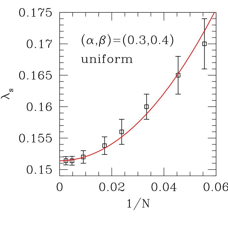
For $(\alpha,\beta)=(0.3,0.4)$, in which case Eq. (3) gives $D^{+}=0.8$, $D^{-}=0.7$ we attempted to fit the exact profiles according to Eqs. (9), (10), and (17) to the form

$$\rho_{s}(\ell)=a+b\,\exp(\lambda_{s}\,(\ell-\ell_{0}))$$ (49)

with $a$, $\lambda_{s}$, and $\ell_{0}$ as adjustable parameters; for $\alpha<\beta$ one keeps $b=+1$ (fixed) as is appropriate for $\alpha+\beta<1$. Results for selected values of $N$ between $15$ and $400$ are displayed in Fig. 2, where the uncertainties shown relate exclusively to the intrinsic features of multiparametric nonlinear regression. The quality of fit improves for increasing $N$, as shown by the shrinking standard deviations for $\lambda_{s}$; also, the central estimates tend to stabilize for $N\gtrsim 100$, suggesting a parabolic form with no linear term in $N^{-1}$ to describe the asymptotic behavior for large $N$ [ shown as a full (red) line in Fig. 2 ]. This gives $\lim_{N\to\infty}\lambda_{s}^{\rm fit}=0.151(1)$, to be compared with the prediction of Eq. (10), $\lambda_{s}^{\rm DW}=0.13353\dots$.

Figure 2: Adjusted values of $\lambda_{s}$ of Eq. (10) for fits of Eq. (49) to exact steady-state profiles, for uniform chains of $N$ sites, against $1/N$. Full line is a parabolic spline through large-$N$ results (see text).

For dynamics, we initially investigated the coexistence line (CL) between low- and high-density phases, at $\alpha=\beta<1/2$, where both $\lambda_{s}$ of Eq. (10) and $\lambda_{d}$ of Eq. (15) vanish. In order to avoid crossover effects due to proximity to the critical point at $(\alpha,\beta)=(1/2,1/2)$ we took $(\alpha,\beta)=(1/4,1/4)$. Keeping only the $n=1$ term in Eq. (12), the very-late time density difference profiles $\delta\rho(\ell,t)\equiv\rho(\ell,t)-\rho_{s}(\ell)$ behave, on the approach to steady-state, as

$$\delta\rho(\ell,t)=-\frac{2(1-2\alpha)}{\pi}\,\sin\frac{\pi\ell}{L}\,e^{-c(L)\,t}\ ,$$ (50)

where the numerical prefactor comes from adjusting the $A_{n}$, $B_{n}$ of Eq. (12) to an empty-lattice initial condition, and the inverse relaxation time is given, using Eqs. (3) and (16) for $L/\pi\gg 1$, by

$$c(L)=R_{1}(L)=\frac{\alpha(1-\alpha)}{1-2\alpha}\left(\frac{\pi}{L}\right)^{2}\ .$$ (51)

Note that Eq. (51) coincides with the Bethe ansatz result of Ref. ess05, [ see their Eq. (22)$\,]$.

For fixed $L$, we ran simulations starting from an empty lattice; then, for a set of suitable $t$ values we fitted numerically generated difference profiles to the sine dependence in Eq. (50), thus producing a sequence of effective time-dependent amplitudes, which was in turn fitted to an exponential time dependence to extract estimates of the $c(L)$ of Eq. (51). Finally, we examined the behavior of the $\{c(L)\}$ against $L$. Results are shown in Fig. 3.

The error bars shown in the Figure result from the cumulative effects of: (i) statistical fluctuations in the local densities for each specified $\ell$ and $t$, coming from the stochastic sampling process; (ii) intrinsic uncertainties following from adjusting difference profiles for fixed $t$ to a single sine dependence while fully neglecting higher-order terms in Eq. (12) [ see Eq: (50) ]; and (iii) additional intrinsic uncertainties related to assuming the time dependence of the effective amplitudes found in (ii) to follow a single exponential form over a relatively broad time interval. We have seen that (ii) and (iii) are of much larger quantitative importance than (i). For instance, the $c(L)$ of Fig. 3 have uncertainties varying between $2$ and $5\%$, while relative fluctuations in the associated difference densities $\delta\rho(\ell,t)$ are of order $1\%$ or less (provided that one analyses sites not very close to the system edges, where the $\delta\rho$ approach zero). Similar considerations apply to the respective sources of the error bars exhibited in Figs. 4, 11, and 12 below.

Figure 3: For $(\alpha,\beta)=(1/4,1/4)$, plot of $L^{2}\,c(L)$ against $1/L$, where the $c(L)$ are adjusted values of the exponential time decay of $\{\delta\rho\}(L)$, see Eqs. (50) and (51). The full (red) line is a linear fit to the data. The long-dashed line marks the DW theory prediction.

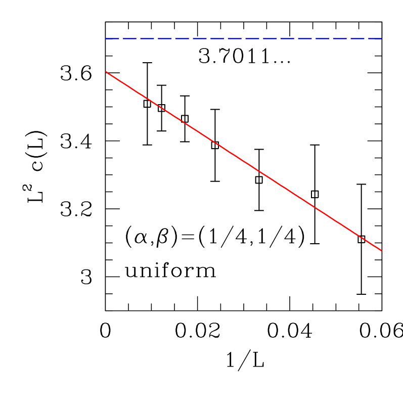
One sees that the numerical estimates of $c(L)$ become closer to the prediction of Eq. (51) with increasing $L$. The extrapolated value is $\lim_{L\to\infty}L^{2}\,c(L)=3.6(1)$, to be compared to $\alpha(1-\alpha)\pi^{2}/(1-2\alpha)=3.7011\dots$ for $\alpha=1/4$.

Next we examined the time evolution of difference densities for $\alpha+\beta<1$, away from the CL. In this case DW theory gives the late-time difference densities as

$$\delta\rho(\ell,t)\propto\exp(\lambda_{d}\ell)\,\sin\frac{\pi\ell}{L}\,e^{-R_{1}(L)\,t}\ ,$$ (52)

with $\lambda_{d}$, $R_{1}(L)$ as given respectively in Eqs. (15) and (16).

At $(\alpha,\beta)=(0.3,0.4)$, using Eqs. (3) and  (16) for $L/\pi\gg 1$ one gets $R_{1}=0.003337\dots+7.3857\dots/L^{2}$. Again, this agrees with the Bethe ansatz result of Ref. ess05, [ see their Eq. (20)$\,]$.

We produced numerical estimates of $R_{1}$ by implementing a procedure similar to that described above for the CL. In contrast to that case, $\lambda_{d}$ is now an additional quantity to be considered. It is known hex15 that the predicted shapes of late-time profiles are very sensitive to the presence of an exponential term in their spatial dependence. Thus, in order to concentrate on the analysis of time decay rates we took $\lambda_{d}$ as an adjustable parameter. However, the following remarks are in order. We saw that (i) for fixed system size $L$, the best-fitting values from numerics systematically decreased for increasing times $t$ in the non-stationary regime; and (ii) while, for assorted $L$ and $t$ one generally found $0.07\lesssim\lambda_{d}^{\rm fit}\lesssim 0.10$, an average over $L$ of long-time extrapolations of the behavior referred to in (i) gives $\langle\lambda_{d}^{\rm fit}\rangle=0.06(1)$. This is to be compared with the prediction $\lambda_{d}^{\rm DW}=0.06676\dots$, and [ using $\lambda_{d}=(1/2)\lambda_{s}\,]$ also to the final result for fits of steady-state profiles to Eq. (49), namely $(1/2)\lambda_{s}^{\rm fit}=0.0755(5)$.

Our results for numerical estimates of $R_{1}$ are shown in Fig. 4.

Figure 4: For $(\alpha,\beta)=(0.3,0.4)$, plot of $R_{1}(L)$ against $1/L$, where the $R_{1}(L)$ are adjusted values of the exponential time decay of $\{\delta\rho\}(L)$, see Eqs. (16) and (52) . The full (red) line is a parabolic fit to the data (see text).

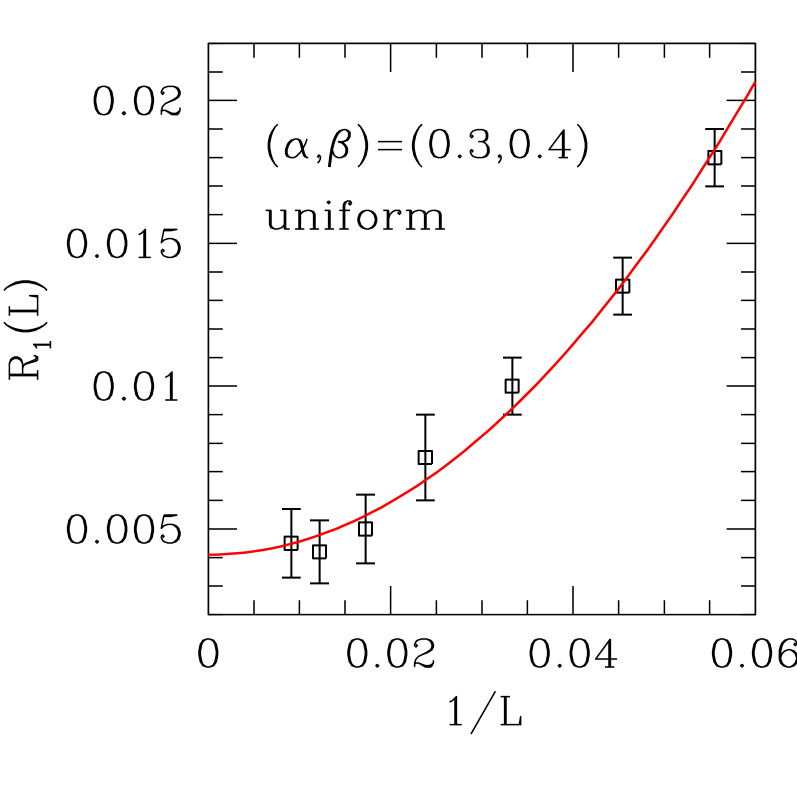
The figure also shows a parabolic fit of the numerical data inspired in the large-$L$ limit of Eq. (16). With $R_{1}(x)=R_{1}^{\,0}+R_{1}^{\,2}\,x^{2}$ one gets $R_{1}^{\,0}=0.0041(4)$, $R_{1}^{\,2}=4.6(2)$, the former value being only two error bars away from the DW prediction.

Still for $(\alpha,\beta)=(0.3,0.4)$ we compared both the stationary and non-stationary behavior of density profiles, as given by DW theory, with corresponding results from, respectively, the exact steady state solution and numerical simulations. To this end, we solved the discrete-time version of Eq. (5),

$$P(\ell,t+dt)=D^{+}dt\,P(\ell-1,t)+D^{-}dt\,P(\ell+1,t)+$$

$$+\left[1-(D^{+}+D^{-})dt\right]P(\ell,t)\ ,\qquad$$ (53)

with similar adaptations to Eqs. (6), (7). Fixing $dt$ amounts to a simple renormalization of the computational time scale with the proviso that the condition $(D^{+}+D_{-})dt<1$ must be obeyed, to prevent negative probabilities cropping up upon iteration. We used $dt=0.5$, which suffices for the present case.

The density profiles can be evaluated at all times via sa02

$$\rho^{DW}(\ell,t)=\left(\sum_{k=0}^{\ell}P_{k}(t)\right)\,\rho^{+}+\left(\sum_{k=\ell+1}^{L}P_{k}(t)\right)\,\rho^{-}\ ,$$ (54)

with $\rho^{+}$, $\rho^{-}$ from Eq. (2).

Fig. 5, for a system with $N=29$ sites, shows the exact steady state profile derr93 compared with two variants of the long-time limit of the evolution of Eq. (53) and the corresponding versions of Eqs. (6), (7). In curve (I) we used $D^{+}$ and $D^{-}$ following Eq. (3), while in curve (II) we took $D^{+}/D^{-}=e^{\lambda_{s}}$, with $\lambda_{s}=0.160$ being the central estimate from the fit of the $N=29$ exact profile to Eq. (49).

Figure 5: For $(\alpha,\beta)=(0.3,0.4)$, $N=29$, points are exact steady-state density profiles derr93 ; lines are results of long-time evolution of Eqs. (5)–(7). (I): $D^{+}$, $D^{-}$ from Eq. (3). (II): $D^{+}/D^{-}=e^{\lambda_{s}}$, $\lambda_{s}=0.160$ (see text).

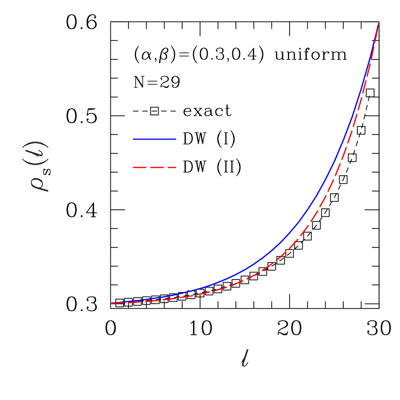
One sees that in both cases, although the general trends are captured by DW results, some small but significant discrepancies remain especially close to the system’s right end. One expects such effects to become less relevant with increasing system size sa02 .

We examined the approach to stationarity, by evaluating the difference densities predicted by DW theory, i.e., $\delta\rho^{\rm DW}(\ell,t)\equiv\rho^{\rm DW}(\ell,t)-\rho_{s}^{\rm DW}(\ell)$. In Fig. 6 they are compared to those coming from simulations. As mentioned previously, the latter use the exact steady state profiles as the baseline to be subtracted from finite-time numerical results.

Figure 6: For $(\alpha,\beta)=(0.3,0.4)$, $N=29$, difference-density profiles. Points are simulation results at $t^{\,\rm sim}=160$. Continuous (red) line is result of evolution of Eqs. (5)–(7) at $t^{\rm DW}=2t^{\,\rm sim}$. The long-dashed line is from MF theory of Ref. hex15 . See text for description of initial conditions.

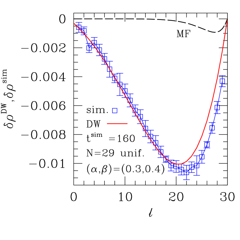
We started the DW evolution with the domain wall at the right end of the system; consistently with this, the numerical simulation was started with uniform average density $\langle\rho\rangle=\rho^{-}=0.3$. With the elementary time step $dt=0.5$ for the DW evolution, as mentioned, the correspondence between times scales is $t^{\rm DW}=2t^{\,\rm sim}$. The features shown in Fig. 6 turn out to be typical of late-time profiles (say $100\lesssim t^{\,\rm sim}\lesssim 250$), namely the very good agreement between DW and simulation results for $\ell\lesssim 20$, and the small but significant mismatch on the upturn for larger $\ell$, with the $\delta\rho^{\rm DW}$ profile approaching zero faster than that given by simulation. The dashed line in Fig. 6 shows the corresponding difference profile predicted by the MF theory of Ref. hex15, . It is seen that there is everywhere a large discrepancy between the latter and simulation results. For a similar (but simpler) case, namely $(\alpha,\beta)=(0.3,0.7)$, see Fig. 7 of Ref. hex15, .

III.3 Staggered chain

We consider chains with alternating rates $p_{1}=1/2$, $p_{2}=1$ for all internal bonds (i.e., excluding the injection and ejection ones). The ratio $p_{2}/p_{1}=2$ is of special interest since its mean-field Mobius mapping description coincides with that of a hexagonal-lattice nanotube with uniform bond rates hex13 ; hex15 . For consistency with the condition expressed above Eqs. (24) and (25), the total number $N$ of sites must be odd.

Eqs. (30), (31), and (32) give, for $p_{1}=1/2$, $p_{2}=1$:

$$\beta=\frac{\alpha}{1+\alpha}\quad{\rm(coexistence)}\ ;$$ (55)

$$\alpha+2\beta=1\quad{\rm(factorization)}\ ;$$ (56)

$$(\alpha_{c},\beta_{c})=\left(\sqrt{2}-1,1-\frac{\sqrt{2}}{2}\right)\quad{\rm(critical\ point)}\ .$$ (57)

As explained in Sec. II.2, the above are concurrent predictions from MF and DW theory. Fig. 7 shows the overall features of the predicted phase diagram in the $\alpha-\beta$ parameter space. In line with the uniform case, one does not expect the continuation of the CL beyond $(\alpha_{c},\beta_{c})$ [ long-dashed line in Fig. 7 ] to have a physical interpretation.

Figure 7: Phase diagram predicted by both MF and DW theory for staggered chain with bond rates $p_{1}=1/2$, $p_{2}=1$; see Eqs. (55)–(57) and text. CL denotes coexistence line; FL is factorization line.

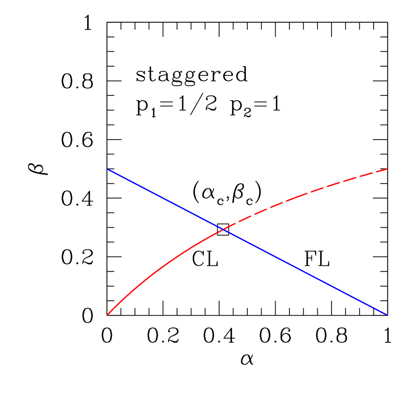
An important feature of driven asymmetric flow on staggered chains hex15 is that no exact results for steady-state profiles or currents are known, e.g., from operator algebra, unlike the case of their uniform-system counterparts derr93 ; thus guidance must come from numerically-generated data. Nevertheless, some general properties which are known for uniform chains are expected to hold here as well, such as the existence of a low-current phase for suitably low ($\alpha$, $\beta$) and a high-current one for ($\alpha$, $\beta$) large enough. For example the steady state current at $(\alpha,\beta)=(1/5,1/6)$, approximately halfway along the predicted CL, is $J\simeq 0.13$. To determine the maximal current $J_{\rm max}$, we considered the simpler case of staggered chains with periodic boundary conditions (rings), for which particle-hole symmetry arguments show that $J_{\rm max}$ corresponds to a site-averaged density $\langle\rho\ \rangle=1/2$. From numerical simulations for system sizes with $\langle\rho\rangle=1/2$, $N=20$, $30$, $40$ one gets $\lim_{N\to\infty}J_{\rm max}(N)=0.1628(1)$, to be compared with the MF prediction $J_{\rm max}^{MF}=p_{1}p_{2}/(\sqrt{p_{1}}+\sqrt{p_{2}})=0.17157\dots$.

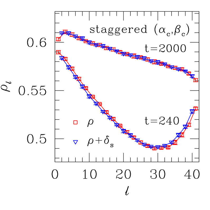
The verification of constant $\ell$-independent difference between sublattice steady state profiles, predicted in Eqs. (47)–(48), is illustrated in Fig. 8. Note that already for $t=240$ there is a good degree of convergence towards a constant difference between sublattice profiles, although some systematic and significant discrepancies still survive. This feature has been found to hold generally for various $(\alpha,\beta)$ spanning all expected phases. The numerical values of the difference $\delta_{s}$ (as defined in Fig. 8) vary in the range $0.04\lesssim\delta_{s}\lesssim 0.15$.

Figure 8: Sublattice density profiles for staggered chain with $N=41$ sites, at ($\alpha_{c},\beta_{c})$ of Eq. (57), starting at $t=0$ with empty lattice. The profile for $t=2000$ corresponds to steady state regime to very good accuracy. Densities for even-numbered sites (blue triangles) have been shifted upwards by $\delta_{s}=0.126$.

We first examined steady-state properties at points well within the predicted low-current phases, i.e. for small $\alpha$, $\beta$ and suitably far from the predicted CL $\beta=\alpha/(1+\alpha)$, $\alpha<\alpha_{c}=\sqrt{2}-1$. We took (i) $(\alpha,\beta)=(0.1,0.22)$ and (ii) $(\alpha,\beta)=(0.3,0.115)$. In both cases DW theory predicts an exponential shape for the sublattice steady-state densities, amenable to fitting via Eq. (49) above, with $b=+1$ for the former, and $b=-1$ for the latter (as they are located on opposite sides of the CL).

From Eqs. (22) and (26) one gets, respectively, $\lambda_{s}=0.65777\dots$ for (i), and $-0.479014\dots$ for (ii). Fitting steady-state profiles from sublattice $1$ for chains with $N=41$ sites to Eq. (49) gives, respectively, $\lambda_{s}^{\rm fit}=0.645(15)$ for (i), $-0.594(8)$ for (ii). Motivated by the uniform-chain case depicted in Fig. 2, in both cases we checked for a systematic $N$-dependence of $\lambda_{s}^{\rm fit}$. We took $N=29$ and $57$. For both $(\alpha,\beta)$ pairs the adjusted parameters stay within at most two error bars from the corresponding $N=41$ values quoted above. So one can conclude that for the former case there is very good agreement between theory and simulation, while in the latter a discrepancy of order $20\%$ is present.

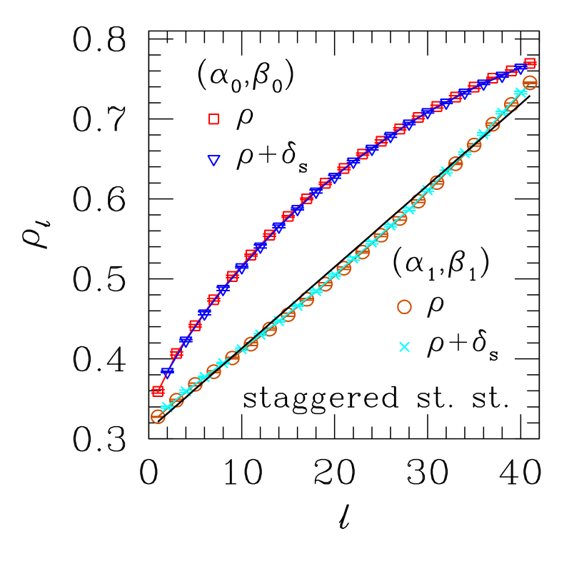
For uniform chains, the coexistence of low-and high- density phases on the CL can be directly observed, see e.g. Fig. 8 of Ref. dqrbs08, ; a secondary characteristic of the CL is that the steady-state (ensemble-averaged) density profile is, to a very good approximation, linear derr93 on it. We have probed the existence of the latter feature for staggered chains, by scanning the $(\alpha,\beta)$ parameter space near the predicted CL. Fig. 9 shows steady state profiles for both $(\alpha_{0},\beta_{0})=(1/5,1/6)$ (on the predicted CL) and at $(\alpha_{1},\beta_{1})=(\alpha_{0}-2\varepsilon,\beta_{0}+\varepsilon)$, $\varepsilon=0.005$. It is seen that at the latter point one gets a rather good fit to a straight-line profile, while there is pronounced curvature at the former. The straight line shown is a least-squares fit to the $(\alpha_{1},\beta_{1})$ data.

Figure 9: Steady state sublattice density profiles for staggered chain with $N=41$ sites, at ($\alpha_{0},\beta_{0})=(1/5,1/6)$ $[\,$on the predicted CL, see Eq. (55) ], and $(\alpha_{1},\beta_{1})=(\alpha_{0}-2\varepsilon,\beta_{0}+\varepsilon)$, $\varepsilon=0.005$. Density values at points on sublattice 2 are shifted upwards by $\delta_{s0}=0.102$, $\delta_{s1}=0.1045$. Straight line is a fit to $(\alpha_{1},\beta_{1})$ data.

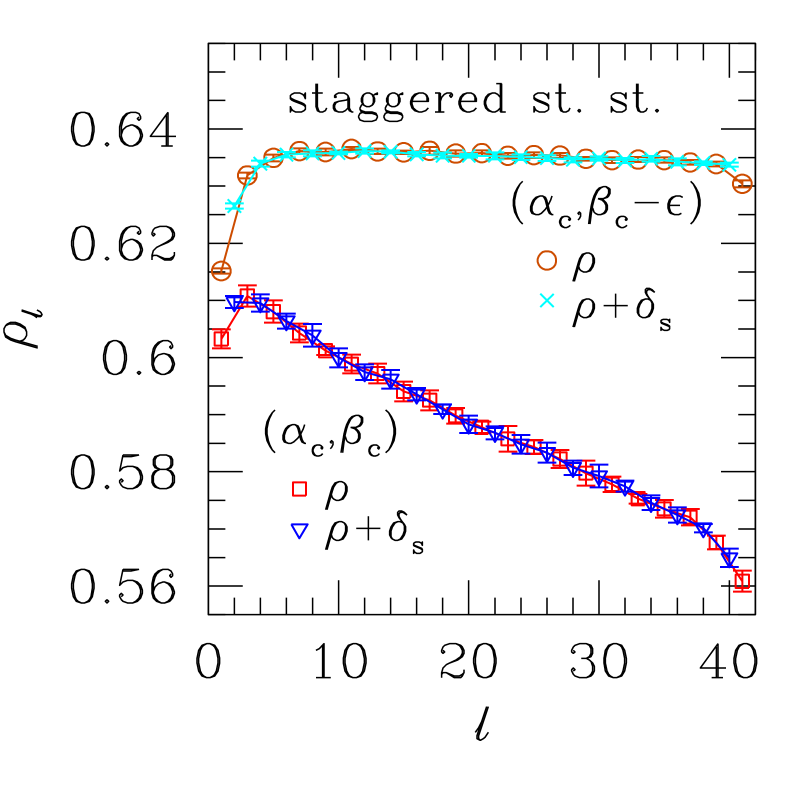
Similarly, for the predicted factorization line on staggered chains, it has been shown by direct evaluation  hex15 that the corresponding correlation functions do not vanish there. For further discussion of this point, see Sec. IV and Appendix A. However, we have seen that a secondary feature, in this case the flatness of steady-state density profiles which holds exactly in the uniform case, can be approximately found close to the predicted location of the critical point, as illustrated in Fig. 10. Leaving out the three leftmost sites, and the rightmost one, on sublattice $1$ of the profile corresponding to $(\alpha_{c},\beta_{c}-\varepsilon)$, which are strongly influenced by the boundary conditions at the chain’s ends, one has a gentle slope for the central section, amounting to a $0.3\%$ density variation in all. This is to be compared with the $6\%$ difference found for the same section of the chain at $(\alpha_{c},\beta_{c})$.

Figure 10: Steady state sublattice density profiles for staggered chain with $N=41$ sites, at the predicted critical point $(\alpha_{c},\beta_{c})$ $[\,$see Eq. (57) ], and $(\alpha_{c},\beta_{c}-\varepsilon)$, $\varepsilon=0.04$. Density values at points on sublattice 2 are shifted upwards by $\delta_{s}=0.126$, $\delta_{s}=0.123$ respectively for $(\alpha_{c},\beta_{c})$, $(\alpha_{c},\beta_{c}-\varepsilon)$ .

For dynamics we used similar procedures to those of Sec. III.2, with pertinent adaptations. For chains with $N=17$, $21$, $29$, $41$, $57$, $81$, and $109$ sites [$\,L=N+1$ bonds ] and late times we evaluated the difference densities $\delta\rho(\ell,t)=\rho(\ell,t)-\rho_{s}(\ell)$. In order to prevent lingering effects of the sublattice fast-equalization process from introducing systematic distortions, we restricted ourselves to sites on sublattice $1$ (odd-numbered). For each of a number (between $5$ and $10$) of suitable sites $\ell$ along the chain, and a set of suitably late times for each site, we fitted the simulation data to a single exponential, thereby producing estimates of the rate $R_{1}=R_{1}(L)$ [ see Eqs. (39)–(44) with $n=1\,$]:

$$\delta\rho(\ell,t)=a(\ell)\,e^{-R_{1}t}\ .$$ (58)

In what folllows, the values used for the numerically-obtained $R_{1}(L)$ are unweighted averages of the exponential-fit results over the several $\ell$’s used.

We first investigated the approach to steady state in the neighborhood of the predicted CL, see Eq. (55), where one expects to find signatures of a gapless spectrum. Motivated by the shapes of steady-state density profiles shown in fig. 9, we took $(\alpha,\beta)=(\alpha_{0}-2\varepsilon,\beta_{0}+\varepsilon)$, with $(\alpha_{0},\beta_{0})=(1/5,1/6)$ on the predicted CL, $\varepsilon=0.005$.

Figure 11: For $(\alpha,\beta)=(\alpha_{0}-2\varepsilon,\beta_{0}+\varepsilon)$, with $(\alpha_{0},\beta_{0})=(1/5,1/6)$ on the predicted CL of Eq. (55), $\varepsilon=0.005$, plot of $R_{1}(L)$ against $1/L^{2}$ where points (blue squares) are adjusted values of the exponential time decay of $\delta\rho(\ell,t)$, see Eq. (58). The full (red) line is a straight-line fit of numerical data for $L\geq 30$ (see text).

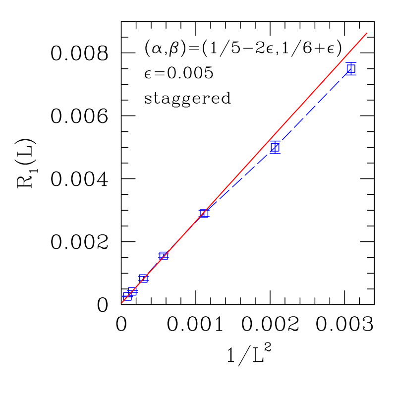
The results for $R_{1}(L)$ are displayed in Fig. 11. The full (red) line $R_{1}=aL^{-2}+b$ shown has adjusted parameters $a=2.60(3)$, $|b|<4\times 10^{-5}$. One sees that for largeish $L\gtrsim 30$, essentially pure $1/L^{2}$ behavior has taken over, as attested by the smallness of $b$. With the diffusion coefficients calculated from Eqs. (26) and plugged into Eqs. (39)–(44) with $n=1\,$, one gets the predicted gap to be $g_{0}=1.83\times 10^{-4}$ at $(\alpha_{0}-2\varepsilon,\beta_{0}+\varepsilon)$, and $\lim_{L\to\infty}(g(L)-g_{0})L^{2}=2.785\dots$, the latter to be compared with the adjusted slope $a$. If one uses instead the parameters at $(\alpha_{0},\beta_{0})$, for which $g_{0}\equiv 0$, the result is $\lim_{L\to\infty}g(L)L^{2}=2.8196\dots$.

We also investigated $(\alpha,\beta)=(0.1,0.22)$, where the agreement between theory and numerics for steady state profiles has proved to be very good (see above). For these values of $(\alpha,\beta)$, Eqs. (26) together with Eqs. (39)–(44) give $g_{0}=0.024907\dots$, and $\lim_{L\to\infty}(g(L)-g_{0})L^{2}=2.2518\dots$. Our numerical results are shown in Fig.12.

Figure 12: For $(\alpha,\beta)=(0.1,0.22)$, plot of $R_{1}(L)$ against $1/L$ where points (blue squares) are adjusted values of the exponential time decay of $\delta\rho(\ell,t)$, see Eq. (58). The (red) triangles are the predictions of Eqs. (26), together with Eqs. (39)–(44) . The dot-dashed (magenta) line is a linear fit to large-$L$ numerical data (see text).

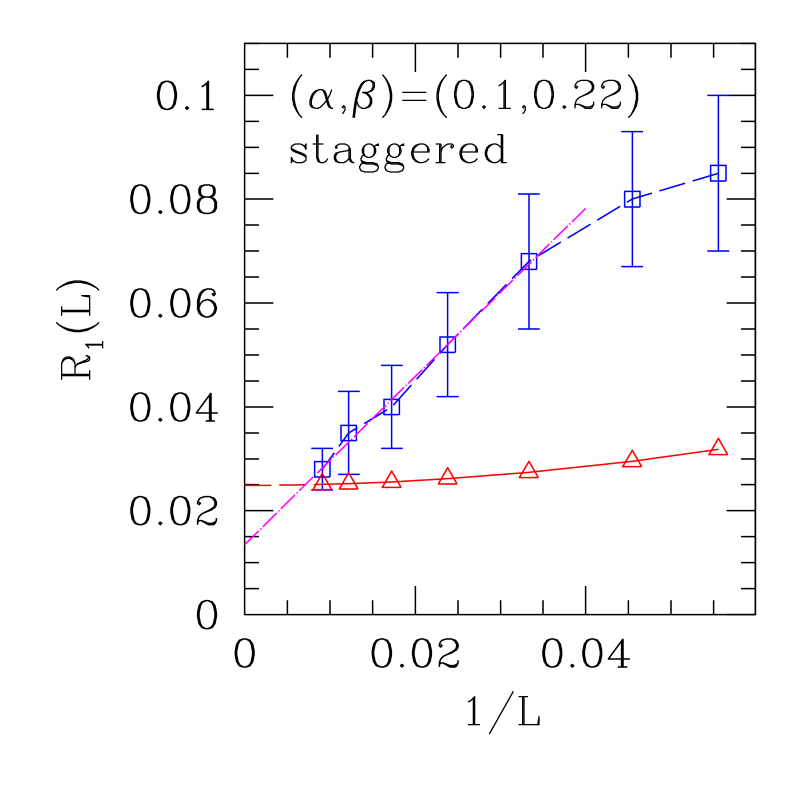
An ad hoc linear fit of the five largest-$L$ data against $1/L$ (shown in Fig. 12) gives $g_{0}=0.013(2)$, albeit with chi-squared per degree of freedom $(\chi^{2}_{\rm d.o.f})=0.03$ due to the rather broad error bars. Assuming that, in qualitative agreement with theory, the asymptotic finite-size correction is in fact $A/L^{2}$ with $A>0$, the above extrapolation for $g_{0}$ can be seen as a loose lower bound for that quantity.

IV Discussion and Conclusions

We initially discuss uniform chains. In general, the results of Sec. III.2 confirm that DW theory is a good approximation. It must be noted, however, that even for steady state some discrepancies remain: see the discussion of numerical data displayed in Figs. 2 and 5. Of course this is because, although the exact steady state profiles (away from factorization and coexistence lines) do behave to a large degree like the exponentials predicted by Eq. (9), they are not identical to them.

Regarding the approach to steady state, DW theory accurately predicts the existence and numerical value of the gap, at least in the low-current phase (and is in accordance with Bethe ansatz results ess05 and simulations, including the main finite-size corrections); see Figs. 3 and 4. The good quantitative agreement between DW evolution and finite-time simulations, already illustrated in Ref. sa02, , is here highlighted and given further prominence by the stark contrast of DW results with the sizable disagreement exhibited by MF treatments against numerics, see Fig. 6 and Ref. hex15, . Indeed, this strongly indicates that fluctuations (incorporated, albeit approximately, by DW theory, and ignored by MF treatments) are the crucial ingredient for the proper description of the approach to steady state.

For staggered chains, we recall that the features of the phase diagram predicted by DW theory coincide with those obtained from application of MF concepts. They are qualitatively similar to those established for uniform chains, exhibiting the special factorization- and coexistence lines along which steady-state density profiles are expected not to display exponential behavior, see Eqs. (22)–(23), (29), and (30).

Numerical evidence that factorization (as characterized by the vanishing of the associated steady-state correlation functions) does not hold as predicted was already found in Ref. hex15, for uniform-rate nanotubes. For such systems the MF Mobius mapping equations are identical to those for the staggered chain with $p_{1}/p_{2}=2$. Here we verified numerically that, similarly, correlations do not vanish for staggered chains, e.g. at $(\alpha_{c},\beta_{c})$ of Eq. (57). Furthermore, by considering suitably short chains, see Appendix A, we were able to prove that there can be no factorizable states except if $p_{1}=p_{2}$.

The proof just referred to adds to the body of evidence displayed in the pertinent results of Ref. hex15, , as well as in Figs. 9 and 10. All the above strongly suggest that for staggered chains the predictions of DW theory regarding factorization, phase coexistence, and criticality come about only in an incipient and quantitatively approximate way.

Notwithstanding the statements just made, we note that DW theory for staggered chains gives reasonably good fits to the steady state exponential $\lambda_{s}$ in regions where it is predicted to differ appreciably from zero, see data for $(\alpha,\beta)=(0.1,0.22)$ and $(0.3,0.115)$. Additionally, the DW theory predictions extracted from Eqs. (47)–(48), regarding $\ell$-independent difference between sublattice steady state profiles, are well verified by numerics; see Figs. 8– 10. In Fig. 8 one can also see evidence of the fast processes having almost completely died out at $t=240$, though convergence toward steady state takes significantly longer.

Concerning the DW description of the approach to steady state for staggered chains, its approximate character is well illustrated by the data shown in Fig. 11. There, we have been able to find a point on the phase diagram, rather close to but not on the predicted coexistence line, where the vanishing of the gap is verified to rather good accuracy. Similarly, the numerically-evaluated coefficient of the leading finite-size correction is within $8\%$ of the DW theory prediction. For an example of a case where the gap is definitely nonzero, namely $(\alpha,\beta)=(0.1,0.22)$ the numerical data exhibit rather broad error bars; nevertheless, with the help of some plausible assumptions one can conclude (see Fig. 12) that the limiting gap value is of the same order of magnitude as predicted by theory, apart from a factor of order $2$ at most.

Before concluding, some further points merit discussion here. The main one concerns length and time scales. For the applicability of the macroscopic view underlying the DW approach one needs an appropriate separation and ordering of such scales, particularly length scales (system size, domain size, domain wall width, and lattice spacing). Such requirements are typically well satisfied in the uniform chain systems investigated here. But for the staggered chains the two-sublattice feature makes them questionable. This may well be the basic reason for the imperfect DW account of this case.

The time scales are important not only for the theory but also in guiding simulations. These scales are set by diffusion rates and bias velocities, together with characteristic lattice or system lengths in gapped or gapless spectra, and lattice traversal times (from real and imaginary parts of the decay rate $R_{1}$). The latter ballistic effects are evident in certain of the current investigations (e.g. in filling of the lattice from the injection side in the case of empty lattice initial conditions, see Fig. 8 above), but have already been detailed elsewhere (see, e.g., Figs. 2, 3, and 5 of Ref. sa02, , as well as Figs. 2 and 7 of Ref. hex15, ).

Appendix A Investigation of possibly factorized steady states

We investigate the possibility of factorized steady states for the staggered chain TASEP using direct application of the transition matrix. The method is feasible for open boundary systems of small size.

We consider systems with $N$ sites, hence $2^{N}$ possible configurations, at small $N$.

We can write down the $2^{N}\times 2^{N}$ transition matrix $\cal W$ whose elements ${\cal W}_{ij}$ give the rates of transition from configuration $j$ to configuration $i$. The ${\cal W}_{ij}$ are functions of the boundary injection and ejection rates $(\alpha,\beta)$ and of the internal hopping rates: $p$ for the uniform case, or $p_{1}$ and $p_{2}$ for the staggered case.

Any state can be written as a column vector in which the $i^{\rm th}$ element, $u_{i}$ say, is the probability of configuration $i$. Steady states have vectors which are eigenvectors of $\cal W$ with zero eigenvalue. So the possibility of a steady state with any sort of factorization can be tested by applying $\cal W$ to its column vector.

For a fully factorizable state the $u_{i}$ can be written in the form $x^{n}\,y^{N-n}$ where $n$ is the number of particles in configuration $i$, and $x+y=1$.

It is easy to check that, for the uniform case at small $N$, such a state is indeed a steady state subject to $\alpha$, $\beta$, $p$ satisfying $\alpha+\beta=p$ and to having $x=1-y=\alpha/(\alpha+\beta)$.

Of course, the exact steady-state solution of the TASEP on a uniform chain derr93 already includes this result. However, nothing comparable is known for the staggered case.

In the latter case the DW approach suggests a steady state which is factorizable on each sublattice, for $a+b=1$, where $a=\alpha/p_{2}$, $b=\beta/p_{1}$.

To verify or refute this, our procedure will be to apply the staggered-chain transition matrix to a corresponding column vector having elements which are products of $x$, $y$, $X$, $Y$, with $x$, $y$ corresponding to particle or vacancy at an odd-index site and $X$, $Y$ likewise for even sites.

Already one obtains conclusive results from size $N=3$. This involves an $8\times 8$ dynamic matrix $\cal W$ which has off-diagonal elements $\alpha$, $\beta$, $p_{1}$, $p_{2}$ or zero, and diagonal elements such that all column sums are zero. Written on a basis in which the first vector element corresponds to all sites occupied, the second element has the first two sites occupied and the last empty, and so on until the last element corresponds to all sites empty, ${\cal W}$ is given by:

$$\begin{pmatrix}{\!-\beta}&{0}&{0}&{\alpha}&{0}&{0}&{0}&{0}\cr{\beta}&{\!-p_{2}\!}&{0}&{0}&{0}&{\alpha}&{0}&{0}\cr{0}&{p_{2}}&{-p_{1}\!-\!\beta}&{0}&{0}&{0}&{\alpha}&{0}\cr{0}&{0}&{p_{1}}&{-\alpha\!-\!\beta}&{0}&{0}&{0}&{0}\cr{0}&{0}&{\beta}&{0}&{\!-p_{1}\!}&{0}&{0}&{\alpha}\cr{0}&{0}&{0}&{\beta}&{p_{1}}&{-p_{2}\!-\!\alpha}&{0}&{0}\cr{0}&{0}&{0}&{0}&{0}&{p_{2}}&{-\alpha\!-\!\beta}&{0}\cr{0}&{0}&{0}&{0}&{0}&{0}&{\beta}&{\!-\alpha}\end{pmatrix}\ \ .$$ (59)

The application of $\cal W$ to the state which is factorizable on each sublattice separately has to give a zero vector for that state to be a steady state. The resulting vector is

$$\begin{pmatrix}{xX(\alpha y-\beta x)}\cr{X[\beta x^{2}-p_{2}xy+\alpha y^{2}]}\cr{x[p_{2}yX+\alpha yY-(p_{1}+\beta)xY]}\cr{x[p_{1}xY-(\alpha+\beta)yX]}\cr{Y[\beta x^{2}-p_{1}xy+\alpha y^{2}]}\cr{y[\beta xX+p_{1}xY-(p_{2}+\alpha)yX]}\cr{y[p_{2}yX-(\alpha+\beta)xY]}\cr{yY(\beta x-\alpha y)}\end{pmatrix}\ \ .$$ (60)

So these elements are all zero only if

$$p_{1}=p_{2}=\alpha+\beta\ ;\ x=X=\frac{\alpha}{\alpha+\beta}\ ;\ y=Y=\frac{\beta}{\alpha+\beta}\ .$$ (61)

This means that the staggered chain with $p_{1}\neq p_{2}$ has no factorizable states, not even with factorization on each sublattice separately.

References

- (1) B. Derrida, Phys. Rep. 301, 65 (1998).
- (2) G. M. Schütz, in Phase Transitions and Critical Phenomena, edited by C. Domb and J. L. Lebowitz (Academic, New York, 2000), Vol. 19.
- (3) B. Derrida, E. Domany, and D. Mukamel, J. Stat. Phys. 69, 667 (1992).
- (4) B. Derrida, M. R. Evans, V. Hakim, and V. Pasquier, J. Phys. A 26, 1493 (1993).
- (5) R. B. Stinchcombe, Adv. Phys. 50, 431 (2001).
- (6) R. A. Blythe and M. R. Evans, J. Phys. A 40, R333 (2007).
- (7) T. Chou, K. Mallick, and R. K. P. Zia, Rep. Prog. Phys. 74, 116601 (2011).
- (8) A. B. Kolomeisky, G. M. Schütz, E. B. Kolomeisky, and J. P. Straley, J. Phys. A 31, 6911 (1998).
- (9) V. Popkov and G. M. Schütz, Europhys. Lett. 48, 257 (1999).
- (10) M. Dudzinsky and G. M. Schütz, J. Phys. A 33, 8351 (2000).
- (11) L. Santen and C. Appert, J. Stat. Phys. 106, 187 (2002).
- (12) R. B. Stinchcombe, S. L. A. de Queiroz, M. A. G. Cunha, and Belita Koiller, Phys. Rev. E88, 042133 (2013).
- (13) R. B. Stinchcombe and S. L. A. de Queiroz, Phys. Rev. E91, 052102 (2015).
- (14) N. Rajewsky, L. Santen, A. Schadschneider, and M. Schreckenberg, J. Stat. Phys. 92, 151 (1998).
- (15) S. L. A. de Queiroz and R. B. Stinchcombe, Phys. Rev. E54, 190 (1996).
- (16) J. de Gier and F. H. L. Essler, Phys. Rev. Lett. 95, 240601 (2005); J. Stat. Mech.: Theory Exp. (2006) P12011.
- (17) S. L. A. de Queiroz and R. B. Stinchcombe, Phys. Rev. E78, 031106 (2008).