BOND: Bayesian Oxygen and Nitrogen abundance Determinations in giant H II regions using strong and semi-strong lines
Abstract
We present bond, a Bayesian code to simultaneously derive oxygen and nitrogen abundances in giant H ii regions. It compares observed emission lines to a grid of photoionization models without assuming any relation between O/H and N/O. Our grid spans a wide range in O/H, N/O and ionization parameter , and covers different starburst ages and nebular geometries. Varying starburst ages accounts for variations in the ionizing radiation field hardness, which arise due to the ageing of H ii regions or the stochastic sampling of the initial mass function. All previous approaches assume a strict relation between the ionizing field and metallicity. The other novelty is extracting information on the nebular physics from semi-strong emission lines. While strong lines ratios alone ([O iii]/H, [O ii]/H and [N ii]/H) lead to multiple O/H solutions, the simultaneous use of [Ar iii]/[Ne iii] allows one to decide whether an H ii region is of high or low metallicity. Adding He i/H pins down the hardness of the radiation field. We apply our method to H ii regions and blue compact dwarf galaxies, and find that the resulting N/O vs O/H relation is as scattered as the one obtained from the temperature-based method. As in previous strong-line methods calibrated on photoionization models, the bond O/H values are generally higher than temperature-based ones, which might indicate the presence of temperature fluctuations or kappa distributions in real nebulae, or a too soft ionizing radiation field in the models.
keywords:
H ii regions – galaxies: abundances – ISM: abundances – methods: data analysis1 Introduction
Thanks to their conspicuous emission lines, giant H ii regions are used as indicators of the chemical composition of the interstellar medium in galaxies, and have permitted important advances in our understanding of the chemical evolution of galaxies (see e.g. Esteban et al., 2004 and references therein). While the so-called temperature-based abundance determinations, which require the measurement of weak auroral lines to measure the electron temperatures, are commonly considered the most reliable, strong-line methods have become increasingly popular since the pioneering studies by Pagel et al. (1979) and Alloin et al. (1979) because they can also be applied for distant galaxies.
Strong-line methods involve some restrictions, though: They assume that giant H ii regions form a one (or two) parameter(s) family and they need to be calibrated. Calibration can be done via a subsample of objects with temperature-based abundances or using a grid of photoionization models. The first method is potentially biased, since calibration samples are likely to have different properties than the samples one wishes to study. In particular, they are biased against objects having intrinsically weak auroral lines. Calibrations based on grids of photoionization models do not have this problem (assuming the models cover all the combinations of important parameters that are encountered in nature and are realistic enough).
A large number of calibrations have been proposed. If we label the methods by their abundance indicators adopting the notation O3N2 for [O iii]/[N ii] 111In the entire paper the notations [N ii], [O ii], [O iii], [Ne iii], [S ii], [S iii], [Ar iii], [Ar iv], and He i stand for [N ii], [O ii], [O iii], [Ne iii], [S ii], [S iii], [Ar iii], [Ar iv], and He i respectively, [O iii]S for 4959 + 5007, and [N ii]S for 6548 + 6584 (where the subscript S is used to denote a sum of emission lines)., O23 for (, N2Ha for [N ii]/H, etc., the most popular ones are: O23 (Pagel et al., 1979), O3N2 (Alloin et al., 1979), O23–O3O2 (McGaugh, 1991), N2Ha (Storchi-Bergmann et al., 1994), S23 (Vilchez & Esteban, 1996). All these methods with their numerous calibrations (here we have quoted the pioneering ones) give very different outcomes (see e.g. Kewley & Ellison, 2008 for a comparison of the results).
Apart from this problem of leading to discrepant results, strong-line methods face two important issues. One is that factors other than just the metallicity and the ionization parameter influence the strength of the strong lines emitted by giant H ii regions. This potentially leads to incorrect inferences when applying the methods to compare different samples (see Stasińska, 2010). The second issue is that there are two regimes where the intensities of the strong oxygen lines used for abundance determinations have the same value with respect to H: the low-metallicity and the high-metallicity regimes. To resolve this bimodality, one uses the intensity of the strong nitrogen line since, in the astrophysical context, the N/O ratio is a function of metallicity. This procedure, a priori reasonable, is however not totally secure since the frontier between the two regimes is fuzzy. For example, McGaugh (1994) adopts while Kewley & Ellison (2008) adopt for the high-metallicity regime. The difference between these two values may appear insignificant but can lead to somewhat different conclusions on metallicity trends within and among galaxies. In addition, this procedure does not allow one to pin down objects with pathological N/O ratios – which may be particularly interesting for unveiling peculiarities in the star-forming histories of galaxies (Mollá & Gavilán, 2010). Apart from peculiar N/O ratios, the N/O vs O/H relation may be different at high redshifts, which would systematically bias metallicity measurements based on the local N/O vs O/H relation for high-redshift galaxies. Of course, methods using directly N/O as an indicator of the oxygen abundance (e.g. the [N ii]/H method proposed by Storchi-Bergmann et al., 1994 or the [N ii]/[O ii] method proposed by Kewley & Dopita, 2002) present the same drawback.
In this paper, we show that using the semi-strong lines [Ne iii], [Ar iii] and He i, in conjunction with the classical strong lines, it is possible to estimate with reasonable accuracy both the oxygen and the nitrogen abundance in giant H ii regions without any prior assumption on the N/O ratio and without the implicit priors of classical strong line methods regarding the ionizing radiation field. The intensities of these semi-strong lines have been listed in many papers reporting on deep spectroscopy of giant H ii regions, so those lines must be present in the spectra for which only the most common strong lines have had their intensities published.
We construct a finely meshed grid of photoionization models varying not only O/H and the ionization parameter as has been done before (McGaugh, 1991; Kewley & Dopita, 2002; Blanc et al., 2015), but also N/O (like Pérez-Montero, 2014). We use this grid to estimate the abundances of O and N in giant H ii regions by means of standard Bayesian inference methods (like Blanc et al., 2015). Unlike Blanc et al. (2015), we do not assume an N/O vs O/H relation, and explicitly explore variations in N/O. The main novelties of our approach are that we consider variations in the hardness of the ionizing field, and that we extract information from semi-strong emission lines in addition to the commonly used strong lines.
The paper is organised as follows. In Section 2 we present the spectroscopic data we have collected from the literature to develop and test our method. In Section 3 we show two extreme versions of the N/O versus O/H diagram obtained from these data using a temperature-based method and using the strong-line method of Pilyugin, Vílchez & Thuan (2010). In Section 4 we present our grid of photoionization models, built using the code Cloudy (Ferland et al., 2013). In Section 5 we present our method, and in Section 6 we show our results for the N/O versus O/H diagram. In Section 7 we provide a summary and elaborate on future directions of work. Three appendices complement this paper. The first one presents a realistic sample of fake sources constructed by selecting model nebulae from our grid. The second one describes a few tests using these fake sources. The third one compares the abundances derived by bond with those obtained by other published methods on the same set of observational data.
2 The observational database
| id | r | name | F3727 | eF3727 | F3869 | eF3869 | … | F7135 | eF7135 | limF4363 | limF5755 |
|---|---|---|---|---|---|---|---|---|---|---|---|
| 001 | a | NGC 1232 02 | 3.9100 | 0.3300 | – | – | … | 0.0610 | 0.0090 | 0.0140 | 0.0140 |
| 002 | a | NGC 1232 03 | 3.3300 | 0.2500 | 0.2530 | 0.0350 | … | 0.0720 | 0.0130 | 0.0260 | 0.0260 |
| 003 | a | NGC 1232 04 | 2.0700 | 0.1700 | 0.2910 | 0.0240 | … | 0.0820 | 0.0090 | 0.0038 | 0.0038 |
| 004 | a | NGC 1232 05 | 2.5300 | 0.1600 | 0.0480 | 0.0060 | … | 0.0650 | 0.0050 | 0.0022 | – |
| … | … | … | … | … | … | … | … | … | … | … | … |
| 705 | z | HSS1809+6612 | 2.5600 | 0.1013 | 0.3150 | 0.0177 | … | – | – | – | – |
| 706 | z | Mrk259 | 2.3900 | 0.0615 | 0.3230 | 0.0099 | … | 0.0820 | 0.0033 | – | – |
| 707 | z | SBS1428 | 1.8800 | 0.0459 | 0.1870 | 0.0059 | … | 0.0600 | 0.0022 | – | – |
| 708 | z | S1657+575 | 2.1300 | 0.0834 | 0.2430 | 0.0157 | … | 0.0740 | 0.0083 | – | – |
2.1 Giant H II regions in spiral galaxies
Data on giant H ii regions in spiral galaxies were gathered from recent medium-resolution high-quality observational studies, mostly with very large telescopes (Keck, VLT) whose high S/N allowed the measurement of auroral lines in at least part of the observed samples. Apart from the large database from van Zee et al. (1998), all the other works involve Bresolin as first or second author, which guarantees a certain homogeneity in the treatment of the data. The following sources were used (the letters correspond the reference labels in Table 1):
-
(a) Bresolin et al. (2005);
-
(b) Bresolin et al. (2004);
-
(c) Kennicutt et al. (2003);
-
(d) van Zee et al. (1998);
-
(g) Bresolin et al. (2009b);
-
(i) Bresolin (2007);
-
(j) Bresolin et al. (2010);
-
(k) Li et al. (2013);
-
(l) Zurita & Bresolin (2012);
-
(m) Bresolin et al. (2012);
-
(n) Goddard et al. (2011);
-
(p) Bresolin et al. (2009a).
All these sources give the line fluxes corrected for extinction and the associated uncertainties. When the intensity of H was not given, it was assumed to be equal to 2.86 times that of H. Many sources list only the intensities of lines that are used in the classical strong lines methods. i.e. [O iii], [O ii] and [N ii]. For papers giving tables with the fluxes of all the lines seen in the spectra, we roughly estimated the upper limits for the intensities of the lines that were not detected, e.g. [Ar iii] or [O iii]. Upper limits are estimated by taking twice the lowest uncertainty in measured lines. This, of course, is a stopgap solution in absence of any direct information from the observers.
2.2 Blue compact galaxies
To increase the number of objects at low metallicities, we use the sample of blue compact galaxies with high quality spectra which were used by Izotov et al. (2007, reference labelled z in Table 1) to derive the pregalactic helium abundance. The abundances of O and N have been recomputed in exactly the same way as for the giant H ii regions in spiral galaxies.
2.3 Subsamples
For the needs of this study, we merge the two samples described above, and then constitute several subsamples.
-
1.
Sample A is constructed from the entire merged sample by selecting all the objects with [O ii], [O iii] and [N ii] available. It contains 708 objects. The line intensities and associated uncertainties are reported in Table 1, available for download from http://bond.ufsc.br.
-
2.
Sample T is the subsample of sample A with available temperature measurements from [O iii] and/or [N ii]; it contains 261 objects.
-
3.
Sample B is the subsample fulfilling the minimum requirements for the use of the bond method, i.e. with available fluxes for [O ii], [O iii] and [N ii] and for the semi-strong lines [Ne iii], [Ar iii] and He i. It contains 156 objects.
3 The observed N/O vs O/H diagram
3.1 Computation of temperature-based O and N abundances
The abundances of O and N were recomputed in a homogeneous way using 5-level atoms for O+, O++and N+. The sources for the collision strengths and transition probabilities are the following222Note that the atomic data used to compute the O and N abundances are the same as the ones entering in the version of Cloudy used to compute our grid of models.. For O ii: Kisielius et al. (2009) and Zeippen (1982); for O iii: Aggarwal & Keenan (1999), Galavis, Mendoza & Zeippen (1997), and Storey & Zeippen (2000); for N ii: Tayal (2011) and Galavis et al. (1997). The electron densities were computed from the [S ii] ratio (when available) using the atomic data from Tayal & Zatsarinny (2010) and Mendoza & Zeippen (1983). When the [S ii] ratio was not available, it was assumed that the electron density is equal to 100 cm-3.
The ionic abundances were computed with a two-zone electron temperature scheme. The temperature derived from [O iii] was used for O++ and the temperature derived from [N ii] was used for O+ and N+. When one of the two line ratios was missing the following classical relation from Garnett (1992) was used:
| (1) |
The O and N abundances were obtained using the classical assumption that oxygen is only in the form of O+ and O++ in the H ii region and that N/O N+/O+.
The uncertainties were estimated by a Monte-Carlo procedure using the uncertainties on the observed line fluxes as described in detail in Stasińska et al. (2013). Uncertainties due to possible deviations from Eq. 1 as well from the N/O N+/O+ equation were not taken into account in the Monte-Carlo procedure.
3.2 Comparison of N/O vs O/H diagrams
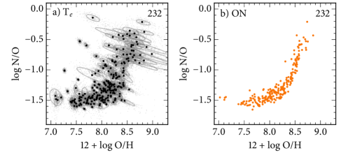
Fig. 1 compares the N/O vs O/H diagram using two different methods for the abundance determination. In the left panel we used the temperature-based method as described above. In the right panel we considered the ON method from Pilyugin et al. (2010), which is based on the [O ii]/H, [O iii]S/H, [N ii]S/H, and [S ii]/H emission line ratios. Both panels show exactly the same 232 objects: From our sample T we select only those objects where [S ii] has been measured, which is necessary for the ON method. This is a strong line method calibrated on a sample of H ii regions with available temperature-based abundances. One can see that the two panels of Fig. 1 look very different, with the left one showing significantly more dispersion than the right one. Note that panel (a) shows some points which are really far away from the main trend, while their associated uncertainties are small.
Which of the two diagrams is closer to reality? Temperature-based methods are often considered the most reliable. However this assertion must be tempered by several considerations. Temperature-based methods assume relations between some parameters (like and or N/O and N+/O+), whereas in fact some dispersion is expected (see Appendix A). They are also strongly dependent on errors in the intensities of the weak lines that serve to determine the temperatures. At the highest metallicities, important temperature gradients inside the H ii regions may bias the abundance results, as shown by Stasińska (2005). Shocks may contribute to the intensities of the auroral lines, and falsify the results on abundances. Finally, if the electron velocities in the ionized gas are not Maxwellian but rather follow a distribution as suggested by Nicholls, Dopita & Sutherland (2012), classical temperature-based methods will result in underestimated abundances with respect to hydrogen. Because of all these reasons, it is not unreasonable to think that part of the scatter observed in Fig. 1 may be artificial. On the other hand, the very tight relation between N/O and O/H seen in Fig. 1 right may be unreal, since the formulae developed by Pilyugin et al. (2010) tend to strongly tighten any preexisting correlation (see Appendix C, Fig. 22).
In what follows, we develop a new method to derive oxygen and nitrogen abundances in giant H ii regions which is much less affected by the intensities of auroral lines than the temperature-based methods and, unlike previous strong line methods, does not involve any assumption on the N/O ratio.
4 The model grid
4.1 Definition of the grid
Because we want to avoid any biases in our method, we need to construct a grid in which we vary all the determinant parameters. If we view a giant H ii region as a nebula powered by an instantaneous burst of star formation, the main parameters for our problem are the oxygen and nitrogen abundances, the mean ionization parameter and the age of the burst. The density distribution may also have a certain importance.
Using Cloudy 13.03 (Ferland et al., 2013), we constructed a grid of models defined as follows.
-
1.
The oxygen abundance on the scale of 12 log O/H goes from 6.6 to 9.4 in steps of 0.2 dex (15 values). The abundances of all the heavy elements except nitrogen and carbon are taken proportional to that of oxygen, as in Stasińska et al. (2015). The helium abundance varies with the oxygen abundances as in Stasińska et al. (2015).
-
2.
The N/O ratio takes the logarithmic values . The abundance of carbon is linked to that of nitrogen by log C/H N/H.
- 3.
-
4.
The mean input ionization parameter, defined by eq. 4 of Stasińska et al. (2015), takes the logarithmic values . Note that the real mean ionization parameter of the computed model is somewhat different from the input value, since it depends on the electron temperature and on the partial absorption of the ionizing photons by dust (see fig. B2 of Stasińska et al., 2015). In the remaining of the paper we denote this mean input ionization parameter as .
-
5.
The starburst age takes the values of 1, 2, 3, 4, 5 and 6 Myr. The spectral energy distribution of the ionizing radiation is obtained from the population synthesis code PopStar (Mollá, García-Vargas & Bressan, 2009) for a Chabrier (2003) stellar initial mass function and for the appropriate metallicity, obtained by interpolation.
-
6.
In order to assess the effect that geometry might have, we consider two density distributions. One is a filled sphere of density , the other is a thin spherical shell of same density. Roughly, the first scenario can correspond to a relatively young H ii region and the second to an evolved one. Clearly these choices are very simplistic and the role of the density distribution should be explored further. The mathematical definitions of the shell and filled sphere are detailed in section 4.1 of Stasińska et al. (2015).
All the models are computed from the inner boundary until the ratio of ionized hydrogen to total hydrogen density falls below 0.02.
4.2 Some characteristics of the grid
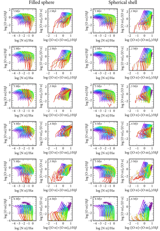
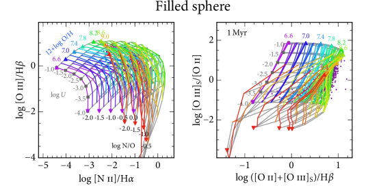
Fig. 2 shows the entire grid of computed models in two planes frequently used to contemplate observations or models of H ii regions. One is the [O iii]/H vs [N ii]/H plane often used for excitation diagnostics (commonly called the BPT diagram after Baldwin, Phillips & Terlevich, 1981), and the other is vs introduced by McGaugh (1991) to derive the oxygen abundance and to which we will refer as the McG diagram. The models for filled spheres are displayed in the left column, while the models for shells are displayed in the right column. Each row of panels corresponds to a given starburst age, increasing downwards. Fig. 3 is a zoom in the BPT and McG planes for the 1 Myr filled sphere subgrid, which serves to better illustrate the coloured lines and points drawn in Fig. 2. Models joined with full coloured lines have the same O/H and same N/O (the colour is defined by the value of O/H and runs from purple to red following the rainbow colours as O/H increases), while models joined with thin grey lines have the same input value of the mean ionization parameter. In all the panels the model curves are superimposed on the observational points.
The first thing we can notice is that the entire grid appears to cover most of the observational points in these two planes, which is what we were looking for, i.e. the fact that the observational points are difficult to see in the figure is a feature, and not a flaw. However, in the McG diagram, a small proportion of objects appears slightly to the right of the grid, at any of the ages considered, meaning that in this region the electron temperature computed by the models is probably lower than in real H ii regions. We have explored several possibilities to reduce the problem by playing with dust and abundance ratios and density, but we did not succeed. Anyway, the discrepancy is much smaller than in the studies of McGaugh (1994) and Dopita et al. (2013, especially for their grid with a distribution of electrons). We think that the discrepancy we find is due to our models still not reproducing exactly real objects rather than to observational errors. Nevertheless, the magnitude of the problem is sufficiently small to warrant our further use of the grid for abundance determinations. Indeed, we find that excluding objects that fall off grid do not change our results.
The two different density distributions (filled sphere and empty shell) produce only slight apparent differences in the grid but, as we will see in Appendix B, this is sufficient to affect the O/H and N/O ratios by up to 0.05 dex. More realistic density distributions, such as a core-halo density distribution or a constant pressure distribution may have a larger impact.
The variations in N/O obviously have an impact on the BPT diagram but they also affect the McG diagram at high metallicities, since they affect the cooling rates. In other words, if the N/O ratio is abnormally high, this would bias the O/H derived from strong-line methods not accounting for a possible scatter in N/O.
We also note that at the highest metallicities the curves of equal chemical composition become ill-behaved. This is because, at such metallicities, most of the cooling occurs through the infrared fine-structure lines whose intensity is not very sensitive to temperature. Therefore a small change in the physical conditions of the gas may alter the electron temperature considerably, which, in turn, strongly affects the intensity of the [O iii] line. This means that, for greater than, say, 9.2, the real error in the abundances derived from optical lines is probably larger than can be estimated from our grid.
Fig. 2 shows that the starburst age modifies the shape of the model grid, especially in the McG diagram, so that assuming the same age for all the H ii regions will produce significant errors in the oxygen abundance determination. What actually changes from one age to another is the ‘hardness’ of the ionizing radiation field, i.e. its capacity of heating the surrounding medium by photoionization.
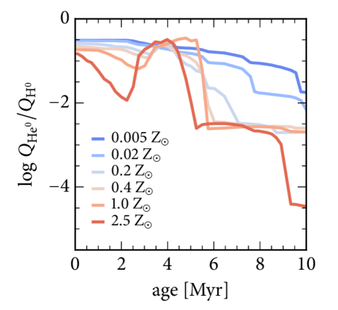
The hardness can be viewed as the ratio /, where is the number of photons above 24.6 eV and is the number of photons above 13.6 eV. Fig. 4 shows the variations of / as a function of time for the six PopStar metallicities. Generally, the ionizing radiation field softens as metallicity increases. However, during the Wolf-Rayet phase the radiation field hardens and this effect is higher at high metallicity. As a result, the radiation field is the hardest at the highest metallicities and at ages around 3–5 Myr. This implies that for these ages the ratio can reach quite high values at high metallicities.
In reality, the process of star formation may not be instantaneous, as in the PopStar models, but extend over a certain time. In practice, what is important for the line intensities is not so much the age of the ionizing stellar population or the regime of star-formation, but rather the hardness of the resulting ionizing radiation field. Our models with different ages should thus be viewed as models for spectral energy distributions of different hardness.
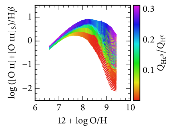
Fig. 5 shows the variations of with respect to O/H for models with , the curves representing the sequences of models being coloured according to the value of /. It is clear that for larger than, say, 7.5, the primary metallicity indicator, , is strongly dependent on /, reinforcing the relevance of considering this effect in the modelling.
5 Description of the BOND method
Our grid of models spans a wide range of physical parameters: N/O, O/H, , the hardness of the radiation sources, and the density profile of the nebula. Although we are only interested in inferring the nitrogen and oxygen abundances, we need to constrain the other nuisance parameters. This section explains our choices of observational constraints and the formalism for our Bayesian Oxygen and Nitrogen abundance Determinations (bond) method.
5.1 Observational constraints
5.1.1 Uncovering N/O and O/H
Our first set of observational constraints are the extinction-corrected line ratios , and . The formal assumption is that those logarithmic line ratios are Gaussianly distributed and independent. Using line luminosities instead of line ratios is meaningless for our models, since the models are not defined by luminosities but by ionization parameters.
The physical reasoning behind using this set of line ratios is that , , and are proxies for N/O, O/H and , respectively. Since we are using only strong lines, there is no constraint on the electron temperature. That way, because vs O/H is bivalued, this first set of constraints finds bivalued solutions for O/H.
We believe that using carefully chosen emission lines is better than using all information available for this problem. We therefore choose not to include [S ii] for two reasons. [S ii] comes from the outskirts of the nebula, which do not coincide with the region where the other strong lines are produced. Any density structure will change [S ii] in relation to the other lines. Second, the S/O ratio in H ii regions could be subject to variations due to different production sites of S and O (e.g. it has recently be proposed by Delgado-Inglada et al., 2015 that intermediate-mass stars could contribute to the global oxygen budget in galaxies) and to different dust-depletion schemes.
5.1.2 Eliminating the bimodality
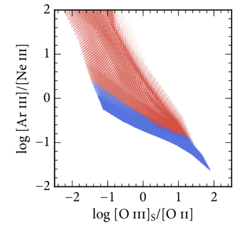
As explained in the introduction, using nitrogen to break the degeneracy with O/H is not satisfactory since the relation between the N/O ratio and O/H is likely dispersed. It is better to use a physical argument that does not depend on astrophysical conditions, like one based on the electron temperature, which will be low in the high abundance regime and high in the low abundance one.
We need a line ratio that is easy to observe, and that depends strongly on the electron temperature and weakly on ionization conditions and abundance ratio. The [Ar iii]/[Ne iii] ratio fulfils these requirements. The [Ar iii] and [Ne iii] lines have different excitation thresholds (1.7 and 3.2 eV, respectively), so different dependencies on the electron temperature. Argon and neon are two primary elements; in addition, they are both rare gases not suspected of dust depletion, so their abundance ratio is expected to be constant. The [Ar iii] and [Ne iii] lines do not arise exactly from the same zone, the ionization potential of Ne++ being higher than that of Ar++, but we can use the [O iii]/[O ii] ratio to figure out what the ionization is.
Fig. 6 shows [Ar iii]/[Ne iii] as a function of [O iii]/[O ii] for our subsample of models corresponding to an age of 2 Myr and a filled sphere nebula. The colours indicate the abundance regime: Blue corresponds to the low metallicity branch in the vs O/H diagram, and red to the high metallicity branch. We can see how using the [Ar iii]/[Ne iii] ratio in conjunction with the [O iii]/[O ii] one separates the two branches. In practice, we use and separately as our constraints because they are closer to an ideal Gaussian distribution than [Ar iii]/[Ne iii]. Also, because the grid was not designed to closely explain [Ar iii]/[Ne iii], we add an extra noise in quadrature to [Ar iii]/H and [Ne iii]/H and marginalise it away, as explained in Section 5.3.1.
The [Ar iii]/[Ne iii] as a function of [O iii]/[O ii] for all starburst ages and scenarios is a bit fuzzier, showing some superposition of high and low metallicity grid points. For those cases, it is useful to include an extra constraint to exclude the grid points on the wrong O/H branch. We find that using the [O iii] and [N ii] upper limits as additional criteria for the electron temperature improves our solutions. The reasoning for using upper limits is that, if the [O iii] (or [N ii]) line is not observed, and the observational upper limit for its intensity is below the expected value in the low metallicity regime, this implies that we are in the high metallicity regime. We include those upper limits in our inference as discussed in Section 5.3.2. We check that this does not force our solutions to match the observed [O iii] or [N ii].
5.1.3 Characterising the radiation field
Line ratios such as ([O iii]/[O ii])/([S iii]/[S ii]) (Vilchez & Pagel, 1988) or ([Ar iv]/[Ar iii])/([O iii]/[O ii]) (Stasińska et al., 2015) can be used to estimate the mean effective temperature of the radiation field. However, [Ar iv] is often too weak to be measured in giant H ii regions. ([O iii]/[O ii])/([S iii]/[S ii]) does depend on (see Stasińska et al., 2015), but, because it depends on [S ii], it suffers from the problem that it is affected by the density distribution in real H ii regions mentioned above (Section 5.1.1).
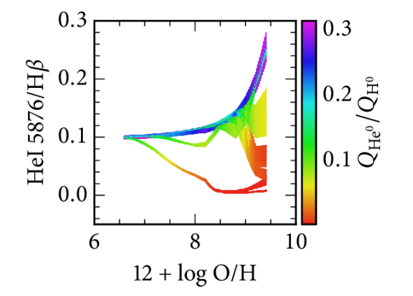
Another potential indicator is He i/H which, as long as helium is not fully ionized in the H ii region, is dependent on the spectral energy distribution of the ionizing stars. The He i/H ratio, however, depends on the metallicity, since the dependence of the He i and H line emissivities with electron temperature is not the same. Fig. 7 shows He i/H as a function of O/H in our grid of models, coloured according to / with the same colour scale as in Fig. 5. We see that, with the information on O/H given by the other lines used in bond, He i/H allows one to estimate / up to a value of 0.2. This is not entirely satisfactory, because Fig. 5 shows that at the highest metallicities, the value of ([O iii]S +[O ii])/H depends on / also at values larger than 0.2. In this paper we restrict ourselves to using He i/H to characterise the hardness of the radiation field. In future works, when large data bases of giant H ii regions with fully described deep spectra become available, it will be possible to add information on [Ar iv]/[Ar iii]. We also allow an extra noise and integrate it out for as described in Section 5.3.1.
5.2 The probabilistic formalism
We aim to find the oxygen and nitrogen abundances of an H ii region by comparing its observed lines to our grid of models. A given observed line is characterised by its intensity and uncertainty (), and an H ii region by its emission lines:
| (2) |
where the curly braces define a set of values spanning the rightmost index (i.e. for the equation above). Each model in our grid is defined by its model parameters , and generates a set of computed line intensities :
| (3) |
Our grid of models spans a wide range of values not only for our two parameters of interest (oxygen and nitrogen abundances), but also for the ionization parameter, starburst ages and nebular geometry. While the latter play an important role in the photoionization modelling of an H ii region, we do not wish to infer them. From a pragmatic point of view, a Bayesian formalism offers a framework to marginalise away those nuisance parameters by simply integrating them out. This comes with the cost of writing down the posterior probability so that the dimensions of our probability function still make physical sense after those integrals are performed (see e.g. Hogg, 2012). The posterior probability density function (PDF) for a model given the observed data and any other relevant background information is
| (4) |
where PDFs are written as , and is a normalisation constant so that the posterior integrates to unity over all the parameter space. The PDFs on the right hand side of the equation are the prior probability of the model parameters, and the likelihood of observing assuming and are true. In what follows we will discuss our generative model for the likelihood and our choice of the prior.
5.3 Generative model for data points
5.3.1 Partially marginalised likelihoods
We assume Gaussian uncertainties for our constraints, which are the logarithmic line fluxes with respect to H. This is a good approximation given that we consider high S/N observations, so that H is very well determined and the line ratios noise uncertainties must deviate very little from a Gaussian distribution. The likelihood of observing an emission line given the model and the background information , plus an extra source of noise with dispersion is
| (5) |
where is a normalisation constant.
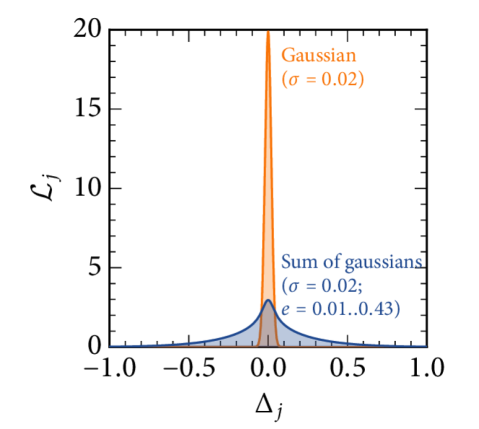
The term was introduced in order to account for deviations in emission line ratios not contemplated in our models. For instance, we use [Ar iii]/H and [Ne iii]/H as constraints, but our models were not meant to reproduce the argon and neon abundance dispersions in nature. For constraints involving strong lines ([N ii], [O ii], [O iii]) we simply set . For constraints based on semi-strong lines ([Ar iii], [Ne iii], He i), we consider in a interval of 0.01 to 0.43 dex (i.e. for an extra noise from 2 to 100 per cent of the measured line intensity). Since we are not interested in , we integrate it out to calculate the marginalised likelihood for :
| (6) |
where is yet another normalisation constant. In practice we calculate as a sum of Gaussians for logarithmically spaced values of . Using only 20 Gaussians for this sum guarantees that the numerical integral with -spaced is equivalent down to to a numerical integral with linear spacing of dex.
Fig. 8 compares a Gaussian with dex (a typical value for the semi-strong lines in our sample) centred in and to a sum of Gaussians with variances , with varying from 0.01 to 0.43 dex. The marginalised likelihood for the sum of Gaussians is much broader than the likelihood for a single Gaussian, but note that it eventually drops to zero. This is an effect brought about by the term in Eq. 5, which penalises very large values of . Therefore, although we allow to vary, the likelihood is still shaped by the data. What happens in practice is that we probe regions of the emission line space in our model grid which are far from the nominal observed measurement.
5.3.2 Treating weak lines
We do not constrain weak line intensities such as [O iii] or [N ii], but we use their upper limits as an additional temperature constraint. The upper limit of the weak line is defined as the 2- detection limit for a given spectrum. The likelihood for weak lines is a step function that masks out models whose computed emission lines are above the upper limit :
| (7) |
This constraint is useful when the [Ar iii]/[Ne iii] ratio alone is unable to distinguish the low and high temperature branches. Imposing an upper limit on [O iii] or [N ii] flags out the solutions for which the temperatures are too high.
This constraint is peculiar, since it is only available for undetected [O iii] or [N ii] lines. Increasing the quality of the observations means that [O iii] and/or [N ii] would be detected and we would not be able to use this constraint any longer. In order to avoid the asymmetry of having this constraint applied for some objects and not others, we impose our upper limit criteria even for sources where [O iii] and/or [N ii] are detected. This procedure also guarantees that higher S/N data are not penalised. We thus assume that the upper limit for a detected line is its intensity plus its 2- uncertainty, which again helps clear out solutions with too high a temperature.
5.3.3 Taking all constraints into account
Assuming that the observed line intensities are independent, the likelihood for all observed line intensities for a given model is
| (8) |
We usually write this down as . Expressing the likelihood in natural logarithmic highlights two points. First, we emphasise that our code adds up instead of multiplying values to minimise numerical errors. Second, we see that, in the case of a fixed extra noise source (constant ), the likelihood reduces to apart from a constant of proportionality. We warn however that the familiar minimisation should be looked with suspicion when applied to abundance determinations. First, when strong and weak lines are all fitted at the same time, weak lines are penalised for having larger uncertainties. Albeit formally correct, this lessens the importance of weak lines while they may carry important information, for example, [O iii] or [N ii], which pin down the electron temperature. Second, the can compensate one badly fitted line with one that is extremely well fitted. The correct way to fit photoionization models would be to fit each line within an appropriate error-bar, which is not ensured by calculating the likelihood by the . To some extent our method is immune to this problem because we only use strong and semi-strong lines as constraints that strongly shape the likelihood, while weak lines are only used as upper limit measurements.
5.4 Adaptive octree grids
The missing piece to calculate the posterior is the prior PDF. Our background knowledge (hence our prior) is encoded in the sampling of our model grid. We follow the reasoning by Blanc et al. (2015) and assume a flat logarithmic prior on O/H, N/O and . This is equivalent to a Jeffrey’s prior for a Gaussian distribution with fixed standard deviation. The age of the ionizing source is linearly sampled, and we have two nebular geometries (a filled sphere and a spherical shell); we assume a flat prior for those.
Our original grid is finely meshed in O/H (0.2 dex), but coarse in all other parameters (0.5 dex in and N/O, 6 starburst ages from 1 to 6 Myr and two nebular geometries). The emission line space is consequently sparsely sampled. When uncertainties in the data are much smaller than the distance between grid models, very few models will be near the observed data. Creating a finer grid can mitigate this problem. Running a sufficient number of photoionization models to fill in the ionizing source ages and nebula density structures adequately would however be unnecessarily time-expensive. Interpolating our grid solves the grid sparsity problem quickly and is a good approximation, since the emission line intensities vary smoothly with those parameters once the initial grid is dense enough. We thus interpolate our original grid in , and , but not in starburst age and geometries, which would be dangerous and meaningless, respectively. A finer grid in the latter parameters would require running more photoionization models, a time-consuming task both for generating the grid and running the bond code. We choose to keep ages and geometries fixed, which pop up as discontinuities and multimodal solutions in our posterior PDFs (take a sneak peek at e.g. the ‘islands’ of solutions in Fig. 11).
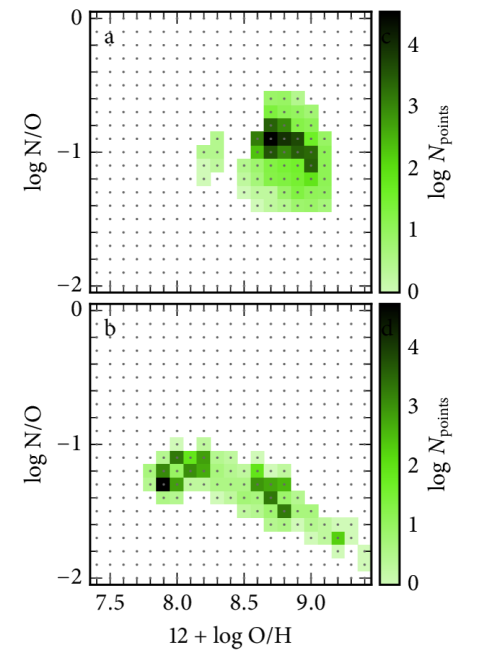
We create a different interpolated grid adapted to each object using an octree sampling algorithm. Octree grids are usually applied to sample a Cartesian 3D space, and are used extensively in video games, computer graphics, hydrodynamics simulations, and Monte Carlo radiative transfer codes (e.g. Saftly et al., 2013 and references therein).
We start off with a grid containing models separated by 0.1 dex in O/H, and N/O. Starburst ages and nebular geometries are kept fixed. Each grid point represents a cell of volume . For each object, we calculate the posterior PDF for all grid points, and the contribution of each grid cell to the total probability.
After this first run, we remove grid cells which contribute too little to to speed up the calculations (the default option is to remove grid points for which considering each age and geometry scenario separately). Grid cells where are subdivided into eight subcells, with each subcell corresponding half the size of the parent cell in O/H, and N/O. The threshold was chosen as a compromise between the precision of the posterior PDF and the computing time. Smaller thresholds create very large octree grids, whilst our nominal solutions (i.e. the posterior summaries, see Section 5.5) for , change by less than 0.02 dex. We recalculate the posterior with the new octree grid, subdivide the cells where needed, and reiterate until there is no remaining cell with above the threshold. This procedure creates a grid that is finer in the parameter space region where the posterior probability is higher.
Fig. 9 shows the final octree grid for two objects in sample B, compressed in the N/O vs O/H space. The dots are the centres of the original 0.1 dex-sampled grid cells, and the green scale represents the final number of subcells. Swathes of white space stand for grid cells that have been removed due to contributing too little to the final probability. For our sample B, the median number of cells is (for a minimum and a maximum of and ), and all the grid cells usually go below the threshold after 6 iterations, which yields subcells times smaller than the original cell (i.e. which span 0.0015625 dex in O/H, N/O and ). The average time to run bond for one source with the octree sampling algorithm in a 1-core 1.7 GHz CPU is 20 seconds.
5.5 Summarising the posterior PDF
Having calculated the full posterior , we can integrate out all parameters we are not interested in and leave out the PDF as a function of only the oxygen and nitrogen abundances. The joint posterior PDF for N/O and O/H (joint PDF for short) is calculated as
| (9) |
where , , , , are the model input parameters log O/H, log N/O, , age and geometry, respectively, and the subscript tags each model in the grid. The sum is made over all models with the same values of log O/H and log N/O, and takes into account the variable octree cell size in . The expectation values for a model input parameter or a computed emission line are given respectively by
| (10) | |||
| (11) |
The bond code computes different summaries for the joint PDF: the maximum a posteriori (MAP, i.e. the point of highest probability of the joint PDF), the central point of the credible regions (i.e., the regions on the N/O vs O/H plane of highest probability) that encompass 5, 50, 68 and 95 per cent of the joint PDF, plus its covariance ellipses (scaled so that its area is the same as that of the credible region).
We also calculate the marginalised posterior PDF for several parameters and emission lines. The marginalised posterior PDFs are summarised by their average, median, and mode (i.e. the peak), plus their dispersion, and the extremes of their 50, 68 and 95 percent equal-tailed (i.e. calculated from the percentiles) and highest density intervals.
For the sake of clarity, in what follows we show our results in three descriptions only: the joint PDF, the maximum a posteriori (MAP) plus the 68 per cent credibility ellipse, and the marginalised median plus the 68 equal-tailed interval. Section 6.2 discusses the differences in the summaries of the posterior PDF.
5.6 A worked example
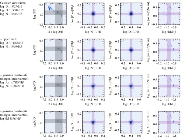
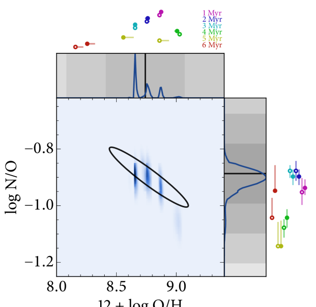
Fig. 10 shows an example of the influence of each set of constraints on the PDFs for an H ii region in NGC 1232. Each row of plots shows the effect of cumulatively adding a set of constraints to the joint PDF of N/O and O/H and to the PDF of the emission line ratios included in the likelihood calculation ([N ii]/H, [O ii]/H, [O iii]/H, [Ar iii]/H, [Ne iii]/H and He i/H). The joint PDF is represented by a blue-scale map. The grey bands mark of the temperature-based values for O/H and N/O, and the purple bands delimit of the observed line ratios.
The top row shows the effect of using , , . A range of solutions pops up in the N/O vs O/H plane, spread out in the high and low metallicity regimes. The second row adds the information on the upper limit detection of [O iii] and [N ii]. This selects the high-metallicity solutions. The third row shows how [Ar iii]/[Ne iii] weighs the four different ‘islands’ of solutions. Those islands correspond to different starburst ages and geometries and are a consequence of the sparsity of our grid in those parameters. The last row shows which solutions are favoured by He i/H, which will be those with the right hardness for the ionizing source. For the [Ar iii]/H, [Ne iii]/H and He i/H ratios, we add an extra noise source and then integrate it out, to account for a dispersion in the Ar/Ne and He/H abundance ratios in real nebulae with respect to the values adopted in the model grid.
This example shows that there are three solutions of about the same probability in the N/O vs O/H plane. Fig. 11 is a zoom of the final N/O vs O/H plane, showing the joint and the marginalised PDFs for N/O and O/H. The dots and lines above the marginalised PDFs are the median and the interval between the 16 to 84 percentiles of the marginalised PDF for each age and geometry combination. Those solutions are displaced from the plot axes for clarity. Spherical shells and filled spheres appear as open and filled circles, respectively, and ages are colour-coded in the rainbow order with 1 Myr ages farther and 6 Myr closer to the axes.
To compare to the Monte Carlo temperature-based realisations, we draw its covariance ellipse on the joint PDF panel, and its , 2 and 3- as grey bands on the marginalised PDFs panels. While the method has not completely eliminated the multimodal nature of the solutions, three out of the four islands of probability on the joint PDF plane are compatible with the temperature-based solution (i.e. inside its covariance ellipse). The multimodal nature of the solutions draws attention to the discreteness of our age grid, as marked by the coloured dots and lines at the edges of the figure. The important message from this plot is that assuming different ionizing fields one finds different values for O/H, and, while He i/H helps pinpointing the right ionizing field, we may still end up with a range of acceptable solutions. This should improve when we have better constraints for the stellar radiation field.
6 Results
6.1 The BOND N/O vs O/H diagram
| id | name | log O/H | log N/O | log O/H | log O/H | … | log O/H | log N/O | log O/H | log O/H | … |
| jmod | jmod | jc68 cen | jc68 sig | mmed | mmed | mp68 low | mp68 upp | ||||
| 002 | NGC 1232 03 | … | … | ||||||||
| 003 | NGC 1232 04 | … | … | ||||||||
| 004 | NGC 1232 05 | … | … | ||||||||
| 009 | NGC 1232 10 | … | … | ||||||||
| … | … | … | … | … | … | … | … | … | … | … | … |
| 704 | F1629+205 | … | … | ||||||||
| 706 | Mrk259 | … | … | ||||||||
| 707 | SBS1428 | … | … | ||||||||
| 708 | S1657+575 | … | … |
We apply our bond method to sample B, which contains 156 objects. Table 2 shows a sample of the summaries for the posterior PDF available to download from http://bond.ufsc.br.
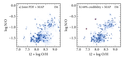
Fig. 12 shows the N/O vs O/H diagram obtained with bond for those objects. The blue points in both panels are the maximum a posteriori (MAP) values for each object. Panel a shows the superposition of the joint PDFs for all objects, while panel b shows the 68% confidence ellipses. Note that some points fall a long way from their ellipses; this is an evidence of multimodal solutions.
We find that our N/O vs O/H diagram is much more dispersed than the one obtained by the ON method of Pilyugin et al. (2010), indicating that in nature this diagram is not a tight sequence. Points are rather spread out like when using temperature-based methods. Naturally part of the spread may be due to imperfections in our models. For instance, we use a simplistic prescription for the nebular density profile, which may not be realistic enough.
Because we do not impose any a priori solution for the N/O vs O/H behaviour, unlike the tight correlation from the grid by Blanc et al. (2015) or the model selection by Pérez-Montero (2014), we find outliers in the N/O vs O/H plane. In Fig. 12 there are at least two objects with low O/H and high N/O in both panels, marked as large red points in panel b (SBS0335-052E and 0837+4717, id numbers 631 and 700 in Table 2). Those objects are likely interesting from a chemical evolution perspective.
6.2 The O/H ratio if one is not interested in N/O
Given that we do not get rid of multimodal solutions, it is to be expected that different ways to summarise the posterior (see Section 5.5) result in different solutions for O/H and N/O. In theory, if one is not interested in N/O, one would be better advised to use the mode, mean or median of the O/H PDF marginalised over N/O, and those are not expected to be exactly the same as the descriptions for the joint PDF.
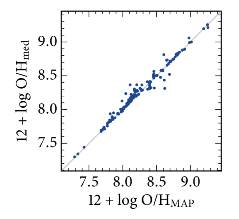
Fig. 13 compares the O/H from maximum a posteriori (MAP) value of the joint N/O vs O/H PDF to the median of the marginalised O/H PDF. For most objects those two solutions agree to within 0.1 dex: There is no bias between those two nominal solutions (the average difference is dex) and the dispersion in small ( dex). Other descriptions of the joint and marginalised PDFs may have a better or worse agreement, but the important point is to always test a few of those descriptions plus their credibility regions.
6.3 Comparison to the direct method
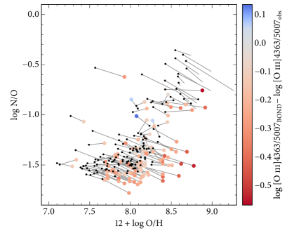
Fig. 14 shows a comparison of bond to temperature-based results for the objects in sample B that have a direct temperature measure. The small black circles are the temperature-based results and the large coloured dots are the bond results. The latter are colour-coded according to the difference between log [O iii]/[O iii] in the models and the observed value (blue for extreme positive values to red for extreme negative values). The bond and temperature-based results for the same H ii region are joined by a solid line.
We see that the bond results generally migrate towards higher values of O/H and lower values of N/O. The colour-coding shows that, for the majority of the points, the bond models have lower temperatures than the observations. This explains why the bond oxygen abundances are higher than the temperature-based ones (typically by 0.2–0.4 dex). Concomitantly, the bond N/O ratios are smaller since the emissivity of the [N ii] line is less dependent on the temperature than that of the [O ii] line, which has a higher excitation threshold.
This problem is not unique either to our grid of models or to our code. Pérez-Montero (2014) only obtains O/H values that are in agreement with the direct method when [O iii] is fitted (see his fig. 2). His method gives a huge weight to [O iii]/H (see his eq. 19); in other words, it becomes essentially a temperature-based method. Blanc et al. (2015) compared the results from their code izi using several photoionization models (Kewley et al., 2001; Levesque et al., 2010; Dopita et al., 2013), and found offsets of to dex with respect to recombination lines, which translate into 0.17–0.56 dex offsets with respect to the temperature-based method.
It is a well-known problem that collisionally excited lines, when using temperature-based methods, lead to lower oxygen abundances than recombination lines (see e.g. García-Rojas & Esteban, 2007), typically by 0.2–0.3 dex in H ii regions. One explanation for this abundance discrepancy problem could be that, in real nebulae, strong temperature fluctuations (Peimbert, 1967; more important than the temperature gradients arising in classical photoionization models) or a distribution of the free electron velocities (Nicholls et al., 2012) boost the [O iii] line, a fact which is not taken into account in the classical temperature-based method nor in the grid of photoionization models we use.
The simplicity of the direct method can be a double-edged sword: although powerful and straightforward to apply, it might be holding too simplistic assumptions as to the production of [O iii].
7 Summary, discussion and future directions
bond determines nitrogen and oxygen gas-phase abundances by using strong and semi-strong lines and comparing them to a grid of photoionization models in a Bayesian framework. The code is written in python and its source is publicly available at http://bond.ufsc.br. The grid of models presented here is included in the 3MdB database (Morisset, Delgado-Inglada & Flores-Fajardo, 2015, see https://sites.google.com/site/mexicanmillionmodels/) under the reference ‘BOND’. The Bayesian posterior probability calculated by bond stands on two pillars: our grid of models and our choice of observational constraints (from which we calculate our likelihoods). We discuss each of these in turn.
The ideal grid of models should be all-encompassing and able to describe any emission-line object found in nature. Creating such a grid would be a daunting and nearly impossible task; therefore we have crafted a set of models that covers enough physical parameters of H ii regions not to be plagued by the usual preconceptions that go into making these grids. Our models span a wide range in N/O and O/H, without imposing any relation between N/O and O/H. The only model grid that has so far taken this approach is the one by Pérez-Montero (2014). Unlike his method, we leave the starburst age and the nebular density structure as free parameters. Finally, a crucial step forward in our approach is taking into account the importance of the hardness of the ionization field. All model grids in the literature consider only a single type of ionizing sources. If the ionization field of the H ii regions differs from those in the models, the O/H obtained will be strongly biased (see the discussion in Appendix B). The hardness of the ionization source may vary due to a few reasons. In local galaxies, the main effects will be the ageing of the stellar populations in H ii regions, and the stochastic sampling of the stellar initial mass function (e.g. Cerviño et al., 2013, and references therein). Our model grid attacks this by using simple stellar populations (SSPs) of different ages for the ionizing sources to account for variations in the ionizing field.
Constructing the grid with great care is not enough. Given the strengths and limitations of our set of models, we need to critically assess which theoretical predictions should be trusted and which observational constraints should go into our fitting procedure. We have set out to infer O/H and N/O, but also to constrain the nuisance parameters , the correct O/H bimodality branch, and the hardness of the ionizing field. The strong lines [O iii]/H, [O ii]/H and [N ii]/H constrain O/H, N/O and . To pin down the correct O/H branch, we use an upper limit in [O iii] or [N ii] when at hand, and the ratio of the semi-strong lines [Ar iii]/[Ne iii], which depends mostly on the electron temperature (modulo the ionizing structure of the nebula, already constrained by [O iii]/[O ii]). Indeed [Ar iii] and [Ne iii] have different excitation thresholds while Ar/Ne in the gas phase is expected to be constant, since both argon and neon are primary elements and inert. Lastly, another semi-strong line comes to rescue: He i/H helps constrain the mean effective temperature of the ionizing radiation field.
Unlike several authors (Dopita et al., 2013; Pérez-Montero, 2014; Blanc et al., 2015) we do not use the [S ii] line in our procedure, first because this line is emitted in the outskirts of H ii regions so that its intensity in relation with [O ii] or [N ii] is dependent on the detailed density structure of the nebulae, second because there might be an intrinsic scatter in the S/O ratio due to stellar nucleosynthesis and/or to depletion effects not yet fully documented.
For a set of giant H ii regions and blue compact dwarf galaxies, we have calculated their gas-phase N/O and O/H abundances and compared them to the ones obtained by the temperature-based method and by the Pilyugin et al. (2010) ON method. We find that the N/O vs O/H relation obtained by bond is as scattered as the one obtained by the temperature-based method, and that the very tight relation obtained with the Pilyugin method is a consequence of that method itself.
We also note that, when using the bond method on objects which have direct temperature measurements, we systematically obtain lower values of [O iii]/[O iii] than observed and higher values of the oxygen abundance than with the temperature-based method. This discrepancy has been seen in many other strong-line methods calibrated on photoionization models and might point to too soft an ionizing spectral energy distribution (SED) in the models. This is in line with the fact that Stasińska et al. (2015), using a subset of our models, found that the SEDs are not hard enough to produce the observed [Ar iv]/[Ar iii] line ratio. It might also indicate that the density distributions of our models are too simplistic to represent real H ii regions. Alternatively, it might be a sign that important temperature fluctuations of unknown origin or a distribution of electron velocities are present in real H ii regions and lead to an overestimate of the temperature indicated by [O iii]/[O iii]. Such an explanation has been suggested by several authors and would at the same time help resolve the famous abundance discrepancy problem (see e.g. García-Rojas & Esteban, 2007; Nicholls et al., 2012; Dopita et al., 2013). Since we do not try reproduce the [O iii] line, nitrogen and oxygen abundances inferred by bond might be more accurate estimates than those of the temperature-based method. Nevertheless, the accuracy of bond abundances strongly relies on how well the photoionization model grid represents real objects.
We have shown that bond, when applying our extensive grid of photoionization models to a well-chosen set of strong and semi-strong lines, allows one to obtain O/H and N/O simultaneously, getting rid of the spectre of bimodality without recourse to empirical oxygen and nitrogen abundance correlations. Our method is very easily extendable and can accommodate many improvements in the future. In spite of many issues still to resolve in the determination of nebular abundances, we hope that bond does offer a quantum of solace.
Acknowledgments
We are thankful to Robert Kennicutt and the referee, Guillermo Blanc, for their insightful comments, which led us to rephrase a number of issues to improve clarity. We also thank Guillermo Blanc for the kindness of running izi for us in the refereeing process. GS and NVA acknowledge the support from the CAPES CsF–PVE project 88881.068116/2014-01. NVA acknowledges the NEBULATOM school held in Choroni, Venezuela, in 2013, and the support and hospitality for short term visits of the LUTH, at Observatoire de Paris. GS and RCF acknowledge the support from the CAPES-COFECUB Te 585/07 project. The grid of models has been run on computers from the CONACyT/CB2010:153985, UNAM-PAPIIT-IN107215 and UNAM Posgrado de Astrofísica projects. This research made use of Astropy, a community-developed core Python package for Astronomy; matplotlib, a Python library for publication quality graphics; SciPy; numpy; h5py; and hickle.
References
- Aggarwal & Keenan (1999) Aggarwal K. M., Keenan F. P., 1999, ApJS, 123, 311
- Alloin et al. (1979) Alloin D., Collin-Souffrin S., Joly M., Vigroux L., 1979, A&A, 78, 200
- Baldwin et al. (1981) Baldwin J. A., Phillips M. M., Terlevich R., 1981, PASP, 93, 5
- Blanc et al. (2015) Blanc G. A., Kewley L., Vogt F. P. A., Dopita M. A., 2015, ApJ, 798, 99
- Bresolin (2007) Bresolin F., 2007, ApJ, 656, 186
- Bresolin et al. (2004) Bresolin F., Garnett D. R., Kennicutt R. C., 2004, ApJ, 615, 228
- Bresolin et al. (2005) Bresolin F., Schaerer D., González Delgado R. M., Stasińska G., 2005, A&A, 441, 981
- Bresolin et al. (2009a) Bresolin F., Ryan-Weber E., Kennicutt R. C., Goddard Q., 2009a, ApJ, 695, 580
- Bresolin et al. (2009b) Bresolin F., Gieren W., Kudritzki R.-P., Pietrzyński G., Urbaneja M. A., Carraro G., 2009b, ApJ, 700, 309
- Bresolin et al. (2010) Bresolin F., Stasińska G., Vílchez J. M., Simon J. D., Rosolowsky E., 2010, MNRAS, 404, 1679
- Bresolin et al. (2012) Bresolin F., Kennicutt R. C., Ryan-Weber E., 2012, ApJ, 750, 122
- Cerviño et al. (2013) Cerviño M., Román-Zúñiga C., Luridiana V., Bayo A., Sánchez N., Pérez E., 2013, A&A, 553, A31
- Chabrier (2003) Chabrier G., 2003, PASP, 115, 763
- Delgado-Inglada et al. (2015) Delgado-Inglada G., Rodríguez M., Peimbert M., Stasińska G., Morisset C., 2015, MNRAS, 449, 1797
- Dopita et al. (2013) Dopita M. A., Sutherland R. S., Nicholls D. C., Kewley L. J., Vogt F. P. A., 2013, ApJS, 208, 10
- Draine (2011) Draine B. T., 2011, ApJ, 732, 100
- Esteban et al. (2004) Esteban C., García López R., Herrero A., Sánchez F., eds, 2004, Cosmochemistry. The melting pot of the elements
- Ferland et al. (2013) Ferland G. J., et al., 2013, Rev. Mex. Astron. Astrofis., 49, 137
- Galavis et al. (1997) Galavis M. E., Mendoza C., Zeippen C. J., 1997, A&AS, 123, 159
- García-Rojas & Esteban (2007) García-Rojas J., Esteban C., 2007, ApJ, 670, 457
- Garnett (1992) Garnett D. R., 1992, AJ, 103, 1330
- Goddard et al. (2011) Goddard Q. E., Bresolin F., Kennicutt R. C., Ryan-Weber E. V., Rosales-Ortega F. F., 2011, MNRAS, 412, 1246
- Hogg (2012) Hogg D. W., 2012, preprint
- Izotov et al. (2007) Izotov Y. I., Thuan T. X., Stasińska G., 2007, ApJ, 662, 15
- Kennicutt et al. (2003) Kennicutt R. C., Bresolin F., Garnett D. R., 2003, ApJ, 591, 801
- Kewley & Dopita (2002) Kewley L. J., Dopita M. A., 2002, ApJS, 142, 35
- Kewley & Ellison (2008) Kewley L. J., Ellison S. L., 2008, ApJ, 681, 1183
- Kewley et al. (2001) Kewley L. J., Dopita M. A., Sutherland R. S., Heisler C. A., Trevena J., 2001, ApJ, 556, 121
- Kisielius et al. (2009) Kisielius R., Storey P. J., Ferland G. J., Keenan F. P., 2009, MNRAS, 397, 903
- Levesque et al. (2010) Levesque E. M., Kewley L. J., Larson K. L., 2010, AJ, 139, 712
- Li et al. (2013) Li Y., Bresolin F., Kennicutt R. C., 2013, ApJ, 766, 17
- Maiolino et al. (2008) Maiolino R., et al., 2008, A&A, 488, 463
- McGaugh (1991) McGaugh S. S., 1991, ApJ, 380, 140
- McGaugh (1994) McGaugh S. S., 1994, ApJ, 426, 135
- Mendoza & Zeippen (1983) Mendoza C., Zeippen C. J., 1983, MNRAS, 202, 981
- Mollá & Gavilán (2010) Mollá M., Gavilán M., 2010, Mem. Soc. Astron. Italiana, 81, 992
- Mollá et al. (2009) Mollá M., García-Vargas M. L., Bressan A., 2009, MNRAS, 398, 451
- Morisset et al. (2015) Morisset C., Delgado-Inglada G., Flores-Fajardo N., 2015, Rev. Mex. Astron. Astrofis., 51, 103
- Nicholls et al. (2012) Nicholls D. C., Dopita M. A., Sutherland R. S., 2012, ApJ, 752, 148
- Pagel et al. (1979) Pagel B. E. J., Edmunds M. G., Blackwell D. E., Chun M. S., Smith G., 1979, MNRAS, 189, 95
- Peimbert (1967) Peimbert M., 1967, ApJ, 150, 825
- Pérez-Montero (2014) Pérez-Montero E., 2014, MNRAS, 441, 2663
- Pilyugin et al. (2010) Pilyugin L. S., Vílchez J. M., Thuan T. X., 2010, ApJ, 720, 1738
- Pilyugin et al. (2012) Pilyugin L. S., Vílchez J. M., Mattsson L., Thuan T. X., 2012, MNRAS, 421, 1624
- Rémy-Ruyer et al. (2014) Rémy-Ruyer A., et al., 2014, A&A, 563, A31
- Saftly et al. (2013) Saftly W., Camps P., Baes M., Gordon K. D., Vandewoude S., Rahimi A., Stalevski M., 2013, A&A, 554, A10
- Stasińska (2005) Stasińska G., 2005, A&A, 434, 507
- Stasińska (2010) Stasińska G., 2010, in G. Bruzual & S. Charlot ed., IAU Symposium Vol. 262, IAU Symposium. pp 93–96
- Stasińska et al. (2006) Stasińska G., Cid Fernandes R., Mateus A., Sodré L., Asari N. V., 2006, MNRAS, 371, 972
- Stasińska et al. (2013) Stasińska G., Peña M., Bresolin F., Tsamis Y. G., 2013, A&A, 552, A12
- Stasińska et al. (2015) Stasińska G., Izotov Y., Morisset C., Guseva N., 2015, A&A, 576, A83
- Storchi-Bergmann et al. (1994) Storchi-Bergmann T., Calzetti D., Kinney A. L., 1994, ApJ, 429, 572
- Storey & Zeippen (2000) Storey P. J., Zeippen C. J., 2000, MNRAS, 312, 813
- Tayal (2011) Tayal S. S., 2011, ApJS, 195, 12
- Tayal & Zatsarinny (2010) Tayal S. S., Zatsarinny O., 2010, ApJS, 188, 32
- Vilchez & Esteban (1996) Vilchez J. M., Esteban C., 1996, MNRAS, 280, 720
- Vilchez & Pagel (1988) Vilchez J. M., Pagel B. E. J., 1988, MNRAS, 231, 257
- Zeippen (1982) Zeippen C. J., 1982, MNRAS, 198, 111
- Zurita & Bresolin (2012) Zurita A., Bresolin F., 2012, MNRAS, 427, 1463
- van Zee et al. (1998) van Zee L., Salzer J. J., Haynes M. P., O’Donoghue A. A., Balonek T. J., 1998, AJ, 116, 2805
Appendix A A Fake sample for tests
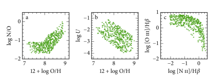
To assess some of the recipes used in temperature-based methods and to test the bond method on objects with known abundances, we construct a ‘fake’ sample by selecting from our grid of models a subsample that roughly follows the expected properties of our observational sample.
To limit the size of our fake sample, we have created an interpolated grid having a resolution of 0.1 dex in O/H and N/O, and 0.5 dex in . We then perturb each cell point in the grid with uniform noise (setting its maximum amplitude to be the size of the cell) in those three input parameters, so that the fake sources are not superimposed in our plots. Our ‘fake’ sources are then chosen to fall roughly in the same loci as observed data, as Fig. 15 shows. We select models in the vicinity of the observed N/O and O/H relation as expressed by eq. 2 of Pilyugin et al., 2012, around the vs O/H relation found by Pérez-Montero (2014), and below the Stasińska et al. (2006) line delimiting pure H ii regions in the BPT diagram. For a given age and geometry we have around – fake sources (except for the 6 Myr scenarios, which fail to cover a large part of the observational data and thus have fake sources).
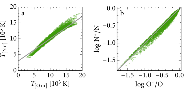
Fig. 16a shows the relation between the temperatures in the high and in the low excitation zones and Fig. 16b shows the relation between the ionic fractions of N+and O+. The temperatures and ionic fractions come directly from the photoionization models for our fake source sample. The continuous lines indicate the relations we used in the temperature-based method. We see that they represent well the trends shown by the models. We also see that the models show some dispersion about these lines. For the temperature the dispersion is of 600 K, while for the logarithm of ionic abundances it is of 0.06 dex.
Appendix B Tests of the accuracy of the BOND method
Here we run a suite of tests fitting models with models, using the same code and the same assumptions as for the sources in sample B. The aim of this exercise is twofold. First, we show that our method works when the input and the output are the same, which is the zeroth test of reliability of any method. Second, we check how the different ionizing source ages and density structures affect our results, since this is the main novelty of our model grid.
The model grid considered is the octree sampled grid. For the tests in this section we select subgrids of single ages and density structures to highlight the effects of those parameters. For all the tests presented here, we assume that the uncertainties in the intensity ratios [O iii]/H, [O ii]/H, [N ii]/H, [Ar iii]/H, [Ne iii]/H, and He i/H are of 10%.
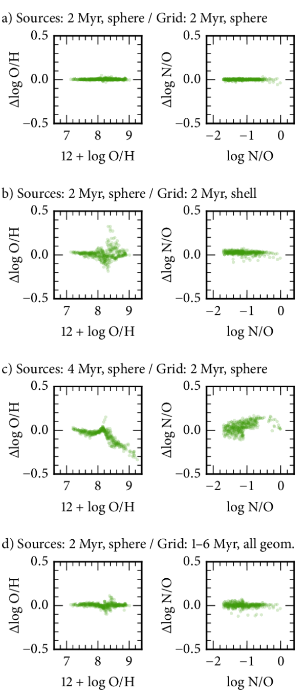
The results of our tests are shown in Fig. 17, where the different rows correspond to different choices of age and geometry. The first row shows 2-Myr starburst and spherical shell fake sources modelled with a grid of the same age and geometry. For O/H and N/O, we show the difference between the output and the input as a function of the input parameter. The results shown are for the maximum a posteriori values. N/O and O/H are well recovered (the dispersion is 0.007 dex).
The second and third rows of Fig. 17 show the effect of using the wrong density structure and age, respectively. The second row shows the 2 Myr filled sphere fake sources fitted with 2 Myr spherical shell models. The residuals for O/H and N/O are very dispersed (0.02 and 0.06 dex respectively) and slightly biased (0.006 and 0.02 dex). The third row shows the effect of using the wrong hardness for the ionization source. Here we have 4 Myr fake sources fitted with a 2 Myr grid, both modelled as filled spheres. This is a very worrying scenario: O/H is underestimated by dex (and up to 0.4 dex) for the high-metallicity branch, while N/O is slightly overestimated (0.04 dex) and rather dispersed (0.05 dex).
The last row shows how our 2-Myr filled sphere fake sources are modelled using our entire grid, i.e. without any a priori knowledge of the geometry and the age of the ionizing source. The results are quite encouraging, and the code seems to choose the right age and geometry combination; or, at least in practice, the right O/H and N/O solution. O/H and N/O are recovered to within better than 0.05 dex (0.02 dex of dispersion).
Appendix C Comparison with other strong line methods
Here we compare our bond method to several other strong line methods. Fig. 18 shows the comparison to the O/H measured by McGaugh (1991), using eqs. A1 and A2 from Kewley & Ellison (2008). The two panels show the effect of choosing different criteria to separate the low and high-metallicity solutions: On the right we use (as in McGaugh, 1994), and on the left (as in Kewley & Ellison, 2008). The separation between the two branches is fuzzy, and the effect of choosing a slightly different frontier is seen when comparing one panel to the other. Focusing on the comparison of McGaugh (1991) to bond, we see a good agreement between the results from bond and those from the much simpler McGaugh recipe, but there are important differences for a non negligible number of sources at high metallicities. There are, as expected, huge differences around , where the O23 ratio is insensitive to metallicity while bond is aided by using the [Ar iii]/[Ne iii] ratio, which steadily increases with increasing metallicity.
McGaugh (1991) was the first to take into account the effect of the ionization parameter when measuring abundances. Fig. 19 shows the comparison of bond results with those using a simple O23 calibration (we have used the one by Maiolino et al., 2008 as an example). The systematics with this simple O23 calibrator are of the order of 0.2–0.5 dex over the whole O/H range.
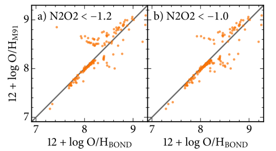
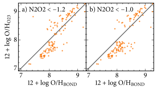
Fig. 20 compares the bond results obtained with our full grid of models to those from the izi code by Blanc et al. (2015) with their default grid (Levesque et al., 2010, 6 Myr constant star formation). Blanc et al. (2015), like McGaugh (1991), assume a N/O vs O/H relation and consider a unique family of ionizing stellar energy distributions. Panel a shows the comparison between the values of O/H derived by bond and izi for the 151 objects in sample B (see Sec. 2.3) which have the izi quality flags npeakZ and limZ equal to one (this removes only 5 objects from sample B). For , izi metallicities are systematically larger than bond by 0.1–0.2 dex. For , the O/H from bond can be 0.3–0.8 dex larger izi for a few objects, while for other objects the codes agree quite well (differing by dex). Panel b of Fig. 20 shows the values of N/O vs O/H derived by bond linked by a straight line to the values obtained by Blanc et al. for the same objects (actually, Blanc et al. determines only O/H, since the N/O values lie on the relation assumed by them). We see that some objects are actually quite far from the tight N/O vs O/H relation assumed, and that for those objects the O/H values derived by bond differ substantially from those derived by Blanc et al.. This illustrates that, for a number of objects (which are not the majority but are not known a priori) it is necessary to simultaneously derive N/O and O/H to obtain a reliable oxygen abundance.
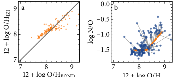
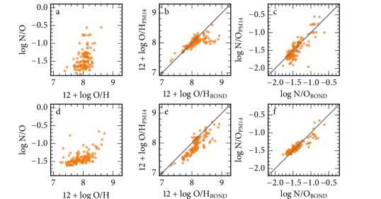
Fig. 21 shows the comparison between bond and the hii-chi-mistry code by Pérez-Montero (2014) for our sample B. We do not show objects that the Pérez-Montero (2014) code flags as bad, i.e. when his grid output is either 2 or 3. From the original 156 objects in sample B, we are left with 129 objects. We use the version 1.2 of his code. The figure shows N/O vs O/H as obtained by the Pérez-Montero (2014) code on the left, and the comparison of the O/H and N/O values to ones obtained by bond on the middle and right panels. The two rows correspond to two different runs of the Pérez-Montero (2014) code. On the top row, we have withheld the [O iii] line from the code, to see how it would behave using only strong lines. This is not the recommended way of running the Pérez-Montero (2014) code, but this exercise shows that it cannot be used as a strong line method. The bottom row shows the results from the Pérez-Montero (2014) code when asking it to fit the [O iii] line as well (with a very strong weight as resulting from his eq. 19). Note that the Pérez-Montero (2014) code finds systematically lower values of O/H than the bond method, exactly like the temperature-based method. The N/O is also rather scattered.
Finally, we use the fake sample of Fig. 15 to show how the ON strong-line method of Pilyugin et al. (2010) biases the abundance results in the N/O vs O/H diagram. As seen in Fig. 22, the ON calibration from Pilyugin et al. (2010) has considerably squeezed the broad input relation.
